CERN-PH-TH/2006-143

TPJU-09/2006

A supersymmetric matrix model:
II. Exploring higher-fermion-number sectors

G. Veneziano

Theory Division, CERN, CH-1211 Geneva 23, Switzerland

and

Collège de France, 11 place M. Berthelot, 75005 Paris, France

J. Wosiek

M. Smoluchowski Institute of Physics, Jagellonian University

Reymonta 4, 30-059 Kraków, Poland

Abstract

Continuing our previous analysis of a supersymmetric quantum-mechanical matrix model, we study in detail the properties of its sectors with fermion number $F=2$ and $3$. We confirm all previous expectations, modulo the appearance, at strong coupling, of two new bosonic ground states causing a further jump in Witten’s index across a previously identified critical ’t Hooft coupling $\lambda_{c}$. We are able to elucidate the origin of these new SUSY vacua by considering the $\lambda\rightarrow\infty$ limit and a strong coupling expansion around it.

CERN-PH-TH/2006-143

TPJU-09/2006

July 2006

1 Introduction

In a previous paper [1] (see also [2] for motivations and details) we have introduced and discussed a new Hamiltonian approach to large-$N$ (planar) theories and have illustrated its effectiveness in a simple supersymmetric quantum-mechanics model. It is the $N\rightarrow\infty$ limit of an $N\times N$ matrix model defined by the following supersymmetric charges and Hamiltonian:

$$Q={\rm Tr}[f{a^{\dagger}}(1+g{a^{\dagger}})]={\rm Tr}[fA^{\dagger}],\;\;\;{Q^{\dagger}}={\rm Tr}[f^{\dagger}(1+ga)a]={\rm Tr}[f^{\dagger}A]\,.$$ (1)

$$H=\{Q^{\dagger},Q\}=H_{B}+H_{F}\,,$$ (2)

$$H_{B}={\rm Tr}[{a^{\dagger}}a+g({a^{\dagger}}^{2}a+{a^{\dagger}}a^{2})+g^{2}{a^{\dagger}}^{2}a^{2}]\,,$$ (3)

$$H_{F} = {\rm Tr}[f^{\dagger}f+g(f^{\dagger}f({a^{\dagger}}+a)+f^{\dagger}({a^{\dagger}}+a)f)$$ (4)

$$+ g^{2}(f^{\dagger}af{a^{\dagger}}+f^{\dagger}a{a^{\dagger}}f+f^{\dagger}f{a^{\dagger}}a+f^{\dagger}{a^{\dagger}}fa)]\,,$$

where bosonic and fermionic destruction and creation operators satisfy:

$$[a_{ij},{a^{\dagger}}_{kl}]=\delta_{il}\delta_{jk}\,,\,\,\{f_{ij}f^{\dagger}_{kl}\}=\delta_{il}\delta_{jk}\,,$$ (5)

all other (anti)commutators being zero.

This dynamical system turned out to be quite interesting per se. Since its Hamiltonian conserves fermion number $F={\rm Tr}[f^{\dagger}f]$, it can be analysed $F$-sector by $F$-sector, with SUSY connecting sectors differing by one unit of $F$. The task of pairing states in supermultiplets is facilitated by the introduction of another conserved operator [1]:

$$C\equiv[{Q^{\dagger}},Q]\,,~{}[C,H]=0\,,~{}C^{2}=H^{2}\,.$$ (6)

Eigenstates of $H$ with eigenvalue $E>0$ can be classified according to their “$C$-parity”, i.e. according to whether $C=\pm E$. We may also consider the combination:

$$C_{F}=(-1)^{F}~{}\frac{C}{E}\,,$$ (7)

a good quantum number for each SUSY doublet. States with $C=+E~{}(-E)$ are annihilated by ${Q^{\dagger}}~{}(Q)$. All the states in the $F=0,1$ sectors turn out to have $C_{F}=-1$ but, in higher-$F$ sectors, there also are some “unnatural” states with $C_{F}=+1$: these are important for the full matching of bosons and fermions.

In [1] we analysed in detail the $F=0$ and $F=1$ sectors of the model. They turn out to provide a complete (although highly reducible) representation of SUSY and to exhibit a number of interesting features. We briefly summarize them hereafter:

• There is a (discontinuous) phase transition, as a function of the ’t Hooft coupling $\lambda\equiv g^{2}N$, at $\lambda=\lambda_{c}=1$. The mass/energy gap, which is present at $\lambda<1$, disappears at $\lambda=1$ and reappears at $\lambda>1$.

• The Witten index [3] (restricted to these two sectors) jumps by one unit at $\lambda=1$ as a result of the appearance, on top of the trivial Fock vacuum, of a new, normalizable zero-energy state at $\lambda>1$. As a consequence, all higher supermultiplets rearrange at the transition point.

• The system exhibits an exact strong–weak duality in its spectrum, with fixed point at $\lambda_{c}$: all excited eigenenergies at $\lambda$ and $1/\lambda$ are connected by a simple relation.

• The spectrum of the model can be computed analytically in terms of the zeros of a hypergeometric function. This makes all the above properties explicit. In particular, the details of the critical behaviour at $\lambda_{c}=1$ can be analysed.

In a subsequent paper [4] some mathematical implications of the pairing of states at arbitrary $F$ and $B$ for the combinatorics of binary necklaces have been discussed. Here we extend the analysis of [1] to the $F=2$ and $F=3$ sectors. As expected, unlike those with $F=0$ and $F=1$, these two higher-$F$ sectors do not provide a complete representation of SUSY (although they contain many of them). In other words, while all $F=2$ states find their SUSY partner in the $F=3$ sector, the reverse is not true: some $F=3$ states have no partner with $F=2$; their partners are expected to lie, rather, in the $F=4$ sector. The quantum number $C$, introduced above, distinguishes the $F=3$ states that have SUSY partners with $F=2$ from those with $F=4$ companions. Thus the linear combinations of $F=3$ fermions that should be degenerate with $F=2$ bosons can be neatly identified, at least for sufficiently weak coupling, and these expectations can be compared with actual numerical calculations.

While we find no surprises at weak coupling ($\lambda<1$), the numerical spectrum at strong coupling ($\lambda>1$) leads to something unexpected: two new zero-energy bosonic states pop up, causing Witten’s index to jump by two units at the $\lambda=1$ phase transition.

The outline of the paper is as follows: in the next section we construct the single-trace (planar) basis with $F=2,3$ and compare it with the $F=0,1$ case discussed in [1, 2]. We also derive explicit expressions for the leading-order matrix elements of the Hamiltonian. The increasing complexity (and some emerging regularities), as we move to higher fermionic sectors, will be emphasized. Section 3 contains the detailed discussion of the physics based on the numerical diagonalization of the planar Hamiltonian. Section 4 provides an analytic construction of the new susy vacua, first at infinite ’t Hooft coupling, and then in the whole strong coupling phase via an expansion in $1/\lambda$. We end by summarizing the main results of this work.

2 $F=2,3$ Fock states and matrix elements at large $N$

Since the Hamiltonian and SUSY charges are simple polynomials in creation and annihilation (c/a) operators, it is advantageous to work in the gauge-invariant eigenbasis of the occupation number operators $B={\rm Tr}[{a^{\dagger}}a]$ and $F={\rm Tr}[f^{\dagger}f]$. At infinite $N$, this basis substantially simplifies. Only states created by single traces of fermionic and bosonic operators give leading-$N$ contributions. For this reason, the $F=0$ and $F=1$ Hilbert spaces were spanned by basis vectors labelled by just a single integer $n$ –the number of bosonic quanta. Extension to higher fermionic sectors is straightforward but requires a little care. A generic state with two fermions has a form

$$|n_{1},n_{2}\rangle=\frac{1}{{\cal N}_{n_{1}n_{2}}}{\rm Tr}[{a^{\dagger}}^{n_{1}}f^{\dagger}{a^{\dagger}}^{n_{2}}f^{\dagger}]|0\rangle,\;\;\;n_{1},n_{2}\geq 0\,,$$ (8)

with a known normalization constant to be discussed shortly. Owing to the cyclic symmetry of the trace, states differing by the interchange of $n_{1}$ and $n_{2}$ are linearly dependent (in fact $|n_{1},n_{2}\rangle=-|n_{2},n_{1}\rangle$ in this case). This fermionic minus sign has yet another consequence: there are no states with $n_{1}=n_{2}$. Therefore the $F=2$ basis can be taken to be

$$|n_{1},n_{2}\rangle,\;\;\;0\leq n_{1}<n_{2}.$$ (9)

Similarly the basis states with three fermions are taken as

$$|n_{1},n_{2},n_{3}\rangle=\frac{1}{{\cal N}_{n_{1}n_{2}n_{3}}}{\rm Tr}[{a^{\dagger}}^{n_{1}}f^{\dagger}{a^{\dagger}}^{n_{2}}f^{\dagger}{a^{\dagger}}^{n_{3}}f^{\dagger}]|0\rangle,\;\;\;\;0\leq n_{1},\;\;\;\;\ n_{1}\leq n_{2},\;\;\;\;\ n_{1}\leq n_{3}.$$ (10)

Notice that cyclic symmetry does not imply any ordering of $n_{2}$ and $n_{3}$. Also, the cases where all (or some) of the bosonic occupation numbers coincide are not excluded in this sector. All the above states are orthogonal in the planar limit, i.e. the off-diagonal elements of the inner-product matrix are subleading.

Matrix elements of the Hamiltonian (2–4) also simplify considerably at infinite $N$. The “planar rules” for obtaining the leading contributions were formulated and illustrated in detail in Refs.[1] and [2]. In short: one uses Wick’s theorem, keeping only the colour contractions that give the maximal number of colour-index loops, hence the highest power of $N$. They come from the planar configurations of all c/a operators, as in the celebrated case of Feynman diagrams [5].

The simplest application of the above rules is the calculation of the normalization factors. One obtains for $F=2$

$${\cal N}_{n_{1}n_{2}}=\sqrt{N^{n_{{\rm tot}}}},$$ (11)

where $n_{tot}=n_{1}+n_{2}+2$ is the total number of quanta in a given state $|n_{1},n_{2}\rangle$.

There is more structure in the three-fermion sector:

$${\cal N}_{n_{1}n_{2}n_{3}}=\sqrt{d}\sqrt{N^{n_{{\rm tot}}}},\;\;\;n_{{\rm tot}}=n_{1}+n_{2}+n_{3}+3,$$ (12)

with the degeneracy factor

$$d=\left\{\begin{array}[]{cc}3&{\rm if}\;\;n_{1}=n_{2}=n_{3},\\ 1&{\rm otherwise}.\end{array}\right.$$ (15)

We are now ready to calculate the complete matrix elements of various terms of the Hamiltonian (2–3). The algebra is straightforward, though a little tedious. We stress that the above normalization factors are crucial. Our final result for the $F=2$ sector reads:

$$\langle n_{1},n_{2}|H|n_{1},n_{2}\rangle=(n_{1}+n_{2}+2)(1+b^{2})-b^{2}(2-\delta_{n_{1},0})-2b^{2}\delta_{n_{2},n_{1}+1},$$ (16)

$$\langle n_{1}+1,n_{2}|H|n_{1},n_{2}\rangle=b(n_{1}+2)=\langle n_{1},n_{2}|H|n_{1}+1,n_{2}\rangle,$$ (17)

$$\langle n_{1},n_{2}+1|H|n_{1},n_{2}\rangle=b(n_{2}+2)=\langle n_{1},n_{2}|H|n_{1},n_{2}+1\rangle.$$ (18)

$$\langle n_{1}+1,n_{2}-1|H|n_{1},n_{2}\rangle=\langle n_{1},n_{2}|H|n_{1}+1,n_{2}-1\rangle=2b^{2}(1-\delta_{n_{2},n_{1}+1})\,,$$ (19)

where, as in [1], we have introduced, for convenience, $b\equiv\sqrt{\lambda}$. Note the $\delta_{n_{2},n_{1}+1}$ exception in the first and last equations. For this configuration of the bosonic occupation numbers Eq. (19) gives rise to a diagonal matrix element. The $\delta_{n_{2},n_{1}+1}$ function prevents double counting of this contribution. Notice also that it comes with the opposite sign to that suggested in Eq. (19). This is because the resulting state $\langle n_{1}+1,n_{2}-1|$ equals minus the state $\langle n_{2}-1,n_{1}+1|$, which belongs to our basis.

In the $F=3$ sector we obtain:

$$\langle n_{1},n_{2},n_{3}|H|n_{1},n_{2},n_{3}\rangle=(n_{1}+n_{2}+n_{3}+3)(1+b^{2})-b^{2}(3-\delta_{n_{1},0}-\delta_{n_{2},0}-\delta_{n_{3},0}),$$ (20)

$$\langle n_{1}+1,n_{2},n_{3}|H|n_{1},n_{2},n_{3}\rangle=\langle n_{1},n_{2},n_{3}|H|n_{1}+1,n_{2},n_{3}\rangle=b(n_{1}+2)\Delta\,,$$ (21)

$$\langle n_{1}+1,n_{2}-1,n_{3}|H|n_{1},n_{2},n_{3}\rangle=\langle n_{1},n_{2},n_{3}|H|n_{1}+1,n_{2}-1,n_{3}\rangle b^{2}\Delta\,,$$ (22)

as well as cyclic permutations of (21), (22), where $\Delta=1/\sqrt{3}$ if $n_{1}=n_{2}=n_{3}$ and $\Delta=\sqrt{3}$ if the final state is of this form; otherwise $\Delta=1$. Similarly to the $F=2$ case, for some sets of $n_{i}$, Eq. (22) gives rise to diagonal elements. However, the $F=3$ Hilbert space is considerably richer that the $F=2$ one and many other “degenerate cases” occur here as well. Instead of dealing explicitly with all these “exceptional” configurations, we adopt a simple, unifying rule:

All contributions listed in (20–22) should be added to the appropriate locations in the $H_{IJ}$ table ($I$ and $J$ are the linear, composite indices labelling all states satisfying (10)).

This rule also covers other “degenerate” situations. For example, for $n_{1}=n_{2}=n_{3}$ the “plus cyclic” qualifier implies that the same matrix element receives an additional factor 3. According to our rule, however, the same elementary matrix element should be added three times, which is of course equivalent.

3 Results

As for the $F=0$ and $F=1$ cases, the complete spectrum with two and three fermions was obtained by diagonalizing numerically the above-mentioned Hamiltonian matrices. To this end, we have introduced a cutoff $B_{{\rm max}}$ that limits the total number of bosonic quanta in the system:

$$B\leq B_{{\rm max}}\,.$$ (23)

Such a cutoff was found very useful in many applications [6], [7], since a) it can be easily implemented in our bases, b) it preserves many symmetries in more complex models, and c) the spectra converge well with increasing $B_{{\rm max}}$.

3.1 Dynamical supermultiplets

The situation is not different in the present case. At $\lambda=2.0$, for example, the lower (i.e. first 20) levels have converged to five decimal digits for cutoffs $B_{{\rm max}}=40~{}(30)$ for $F=2~{}(3)$. Figure 1 compares the spectra in all four fermionic sectors, displaying clearly similarities and differences between the $F=0,1$ and the $F=2,3$ cases. Supersymmetry, which is broken by the cutoff, is nicely restored – there is an excellent boson fermion degeneracy already at the above or higher values of $B_{{\rm max}}$. Interestingly, while all $F=0$ states had their supersymmetric counterparts in the $F=1$ sector and vice versa, for higher fermionic numbers this is not so. Every state with $F=2$ has its partner in the $F=3$ sector, but the reverse is not true: some states with $F=3$ are “unpaired” in Fig. 1 and, consequently, must have their counterparts in the $F=4$ sector. This is already expected at the level of counting basis states in respective Hilbert spaces; however, Fig. 1 provides a clear dynamical confirmation of this structure.

Figure 1: Low-lying bosonic and fermionic levels in the first four fermionic sectors.

Apart from supersymmetry, the spectra in higher-$F$ channels are obviously much richer than those for $F=0,1$. In fact in all earlier cases we know of, the energy levels were almost equidistant in the large-$N$ limit [8],[9]. This also happened for $F=0,1$ in our model, possibly suggesting some generic simplification of planar dynamics, but is no longer true with more fermions. In fact, some levels are so close that they seem to merge into one because of the poor resolution of the graph (e.g. the levels # 4,5 with $F=2$ and # 4,5 with $F=3$). Interestingly, both members of the $\#4,5$, $F=2$ doublet find their partners within the $F=3$ sector. However, this is by no means a general rule (cf. # 10,11 with $F=3$ ).

3.2 Phase transition, rearrangement and new SUSY vacua

One of the remarkable features of our system, seen also analytically in the $F=0,1$ sectors, was the phase transition at $\lambda=\lambda_{c}=1$. At this point the spectrum became gapless, and a critical slowing down of the cutoff dependence was observed. The same phenomenon occurs in the $F=2$ and $F=3$ sectors. In Fig. 2 we show the $\lambda$ dependence of the few lowest levels, with two and three gluinos. The critical slowing down of the convergence is clearly observed. Close to the critical point, supersymmetry is visibly broken, at fixed $B_{{\rm max}}$, while away from $\lambda=1$ supermultiplets are well formed.

Interestingly, SUSY partners rearrange themselves across the phase-transition point, as in the $F=0,1$ case. A novel feature, however, is that, in the strong coupling phase, two zero-energy states appear in the $F=2$ sector. This is to be compared with the $F=0$ case where the trivial Fock vacuum (present at all $\lambda$) is accompanied by a second $E=0$ state in the strong coupling phase.

The claim that all the curves in Fig. 2 converge to zero at $\lambda=1$ may seem a little premature. However, we have repeated our analysis for a few values of $B_{{\rm max}}$ and established that this is the most likely scenario. This point is now being carefully and quantitatively studied by P. Korcyl. The analytic results discussed in the next section also confirm this conclusion.

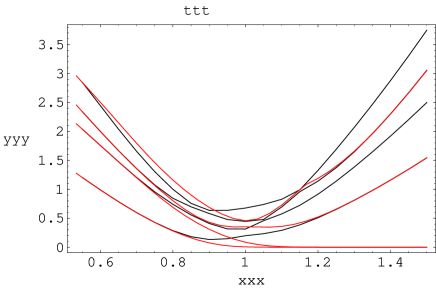
Figure 2: Rearrangement of the $F=2$ (red) and $F=3$ (black) levels while passing through the critical coupling $\lambda_{c}=1$; $B_{{\rm max}}=30~{}(25)$ for $F=2~{}(3)$.

3.3 Supersymmetry fractions

Apart from the unbalanced vacua and boson–fermion degeneracies of higher states, supersymmetry manifests itself in yet a different but important way. Namely, the supersymmetry charges $Q$ and ${Q^{\dagger}}$ transform members of the supermultiplets into each other. Since our method provides not only the eigenenergies, but also the eigenstates, we can directly check these relations. To this end define the “supersymmetry fractions” [7]

$$q_{mn}=\sqrt{\frac{2}{E_{n}+E_{m}}}\langle F=3,E_{m}|{Q^{\dagger}}|F=2,E_{n}\rangle,$$ (24)

which are the, suitably normalized, coordinates of the supersymmetric image of the $n$-th, $F=2$, eigenstate in the $F=3$ sector. For unbroken supersymmetry, $q_{mn}=\delta_{mn}$ (with an appropriate labelling of the $F=3$ states). For finite cutoff, however, the supermultiplets are not yet well formed and $q^{\prime}s$ are not unity . Figure 3 shows the cutoff dependence of the first few supersymmetry fractions. For low cutoffs they can vary rather irregularly until the partner is rapidly found and convergence takes place up to a small noise.

Figure 3: First five supersymmetry fractions, defined as $q_{n}={\rm Max}_{m}(|q_{mn}|)$, for a range of cutoffs.

3.4 Restricted Witten index

The effect of the new SUSY vacua on the Witten index is best seen if we restrict the sum

$$W(T,\lambda)=\sum_{i}(-1)^{F_{i}}e^{-TE_{i}}$$ (25)

to the states in the $F=2$ and $F=3$ sectors and exclude the $C=-E,F=3$ states. In practice we have used the supersymmetry fractions and identified the SUSY partners for each of the $F=2$ states. This procedure, performed necessarily at finite cutoff, is unambiguous away from the transition point. Close to $\lambda_{c}$, however, supersymmetry is badly broken at any finite $B_{{\rm max}}$, and a definition of what is meant by the “energy of the supersymmetric partner” must be given. We made the following choice:

$$W_{R}(T,\lambda)=\sum_{i}\left(e^{-TE_{i}}-e^{-T\bar{E}_{i}}\right),\;\;\;\bar{E}_{i}=\frac{\sum_{f}E_{f}|q_{fi}|^{2}}{\sum_{f}|q_{fi}|^{2}}\,,$$ (26)

where the $i(f)$ indices run over all states in the $F=2~{}(3)$ sectors. In another words, we take for the energy of the partner the weighted average over all $F=3$ states with the weight given by the supersymmetric fractions. Away from $\lambda_{c}$ this selects the true supersymmetric partners and automatically excludes the $C=-E,F=3$ states. The index defined in this way is a smooth function of the ’t Hooft coupling (see Fig. 4) showing the onset of the discontinuity caused by the new vacua in the strong coupling phase.

Figure 4: Behaviour of the restricted Witten index, at $T=6$, around the phase transition. The various curves correspond to $8\leq B_{{\rm max}}\leq 14$.

4 Explicit construction of the strong-coupling vacua

The (numerical) appearance of two new SUSY vacua above $\lambda=1$ was quite unexpected. In order to understand their origin we first consider the limit of infinite ’t Hooft coupling. As we will see, the necessity of two new vacua comes out very simply at $\lambda=\infty$. The corresponding eigenvectors also greatly simplify in that limit (they have projections only on one or two Fock states). We will then show, by an explicit construction, that those vacua persist even at finite (but sufficiently large) $\lambda$, although the corresponding eigenvectors will contain an infinite superposition of Fock states.

We wish to mention that the $\lambda\rightarrow\infty$ limit also simplifies the discussion of our model at arbitrary $F$, since the Hamiltonian becomes block-diagonal with finite-dimensional blocks. Furthermore, some restricted supertraces can be used to identify (and/or guess) the blocks where new SUSY vacua are expected. This result was exploited in Ref. [4] and will be described in more detail elsewhewe.

4.1 SUSY vacua at infinite $\lambda$

The limit $\lambda\rightarrow\infty$ of our Hamiltonian is actually infinite. However, we can define appropriately rescaled SUSY charges that have a finite limit and that, consequently, define a finite rescaled Hamiltonian. Of course eigenvectors will be invariant under such an overall rescaling. The strong-coupling limit of our rescaled SUSY charges reads simply:

$$Q_{\rm{strong}}=\lim_{\lambda\rightarrow\infty}\frac{1}{\sqrt{\lambda}}Q=\frac{1}{\sqrt{N}}{\rm Tr}({a^{\dagger}}^{2}f),\;\;\;\;Q_{\rm{strong}}^{\dagger}=\lim_{\lambda\rightarrow\infty}\frac{1}{\sqrt{\lambda}}{Q^{\dagger}}=\frac{1}{\sqrt{N}}{\rm Tr}(a^{2}f^{\dagger}).$$ (27)

The peculiar property of these charges is that they change $F$ and $B$ but preserve the combination $2F+B$ (unlike the zero-coupling charges that preserve $F+B$). In other words, if we represent our base states on a grid having coordinates $F$ and $F+B$, the infinite $\lambda$ charges connect states along a 45-degree diagonal (while the zero-coupling charges connect states on lines parallel to the $F$ axis). A necessary condition for having no zero-energy states along these diagonals is that the corresponding supertrace be zero. Conversely, if the supertrace is non-zero, there must be some unpaired SUSY vacua lying on those diagonals.

A very simple inspection immediately shows that the latter is the case for the diagonal that contains the state with $F=0$ and $B=1$ (the strong coupling vacuum of [1]) as well as for those that contain either the $F=2,B=1$ or the $F=2,B=3$ states. The latter are our new SUSY vacua at infinite $\lambda$.

Let us now consider the infinite $\lambda$ limit of the (rescaled) Hamiltonian (2)–(4):

$$H_{\rm{strong}}=\lim_{\lambda\rightarrow\infty}\frac{1}{\lambda}H=\frac{1}{N}{\rm Tr}[{a^{\dagger}}^{2}a^{2}+f^{\dagger}af{a^{\dagger}}+f^{\dagger}a{a^{\dagger}}f+f^{\dagger}f{a^{\dagger}}a+f^{\dagger}{a^{\dagger}}fa]\,.$$ (28)

This result can be simplified further, providing a good illustration of our planar rules. Namely, the third and fourth terms must be brought to the normal form. Explicitly

$$f^{\dagger}_{ij}a_{jk}{a^{\dagger}}_{kl}f_{li} = f^{\dagger}_{ij}({a^{\dagger}}_{kl}a_{jk}+\delta_{jl}\delta_{kk})f_{li}=N{\rm Tr}[f^{\dagger}f],$$ (29)

$$f^{\dagger}_{ij}f_{jk}{a^{\dagger}}_{kl}a_{li} = f^{\dagger}_{ij}{a^{\dagger}}_{kl}f_{jk}a_{li}=0\,,$$ (30)

since the neglected terms do not yield a single trace. The strong-coupling Hamiltonian thus reads

$$H_{{\rm SC}}=f^{\dagger}f+\frac{1}{N}{\rm Tr}[{a^{\dagger}}^{2}a^{2}+{a^{\dagger}}f^{\dagger}af+f^{\dagger}{a^{\dagger}}fa]\,.$$ (31)

Remarkably, it conserves both $F$ and $B$.

4.2 Strong-coupling vacua from infinite-coupling vacua

In the $F=0$ sector we were able to give an explicit construction of the non-trivial vacuum at $\lambda>1$. Actually, the new zero-energy state could be written down for any value of $\lambda$ but was only normalizable in the strong-coupling region. We may ask whether a similar analysis can be carried out in the $F=2$ sector. The $F=0$ and $F=2$ sectors share the property that all their states are annihilated by $Q$. Therefore, null states with $F=0,2$ are characterized by the fact that they are annihilated by ${Q^{\dagger}}$. Indeed, the $F=0$ null state can be easily obtained in this way by writing:

$$Q = Q_{w}+Q_{s}\,,\,~{}{Q^{\dagger}}={Q^{\dagger}}_{w}+{Q^{\dagger}}_{s}\,,\,$$

$$Q_{w} = {\rm Tr}[f{a^{\dagger}}]\,,\,~{}Q_{s}=g{\rm Tr}[f{a^{\dagger}}^{2}]\;\;\;{Q^{\dagger}}_{w}={\rm Tr}[f^{\dagger}a]\;,\;\;{Q^{\dagger}}_{s}=g{\rm Tr}[f^{\dagger}a^{2}]\,,$$ (32)

where the labels $w$, $s$ refer to the weak and strong coupling forms of the supersymmetric charges, respectively. Note that $\{Q_{w},Q_{s}\}=0$ and that, if we define $H_{w}=\{Q_{w},{Q^{\dagger}}_{w}\}$, $H_{s}=\{Q_{s},{Q^{\dagger}}_{s}\}$, we also have $[H_{w},Q_{w}]=[H_{s},Q_{s}]=0$, and similarly with $Q\rightarrow{Q^{\dagger}}$.

Given the action of ${Q^{\dagger}}_{w}$ and ${Q^{\dagger}}_{s}$ on $F=0$ states:

$${Q^{\dagger}}_{w}|n\rangle=\sqrt{n}|n-1,F=1\rangle\,,\,~{}{Q^{\dagger}}_{s}|n\rangle=b\sqrt{n}|n-2,F=1\rangle\,,$$ (33)

we see immediately that:

$$|v,F=0\rangle=\sum_{n=1}^{\infty}\frac{(-b)^{-n}}{\sqrt{n}}|n\rangle$$ (34)

is annihilated by ${Q^{\dagger}}$. Clearly, it is normalizable only for $b>1$.

A very similar construction works for one of the two strong-coupling ground states. Let us look indeed for a state consisting of a linear superposition of $F=2$ states of the form:

$$|v,F=2\rangle_{1}=\sum_{n=1}^{\infty}c_{n}|0,n\rangle\,.$$ (35)

This time we find:

$${Q^{\dagger}}_{s}|0,1\rangle=0~{},~{}{Q^{\dagger}}_{w}|0,n\rangle=b^{-1}{Q^{\dagger}}_{s}|0,n+1\rangle\,,$$ (36)

and therefore a zero-energy state is simply:

$$|v,F=2\rangle_{1}=\sum_{n=1}^{\infty}(-b)^{-n}|0,n\rangle\,.$$ (37)

Note that the above state is written as a Taylor series in $1/b$ starting from one of the two infinite-coupling ground states:

$$|v,F=2\rangle_{1}^{\infty}=|0,1\rangle\,.$$ (38)

Like its analogue in the $F=0$ sector, this null state is only normalizable if $b>1$.

For a second independent $E=0$ state, let us start our series from the other infinite-coupling vacuum:

$$|v,F=2\rangle_{2}^{\infty}\equiv|0,3\rangle-2|1,2\rangle\rightarrow\,|v,F=2\rangle_{2}$$ (39)

and use the following theorem:

Given an $F=2$ state annihilated by ${Q^{\dagger}}_{s}$ (e.g. (39)) the state:

$$|v,F=2\rangle_{2}\equiv\left(1+Q_{s}H_{s}^{-1}{Q^{\dagger}}_{w}\right)^{-1}|v,F=2\rangle_{2}^{\infty}$$ (40)

is annihilated by ${Q^{\dagger}}$ and is therefore a null state.

The proof is easily carried out by expanding the fraction in powers of $1/b$ (NB: $Q_{s}H_{s}^{-1}=O(1/b)$) and by noting that the first term is annihilated (by construction) by ${Q^{\dagger}}_{s}$ while the other terms cancel pairwise. Indeed:

$${Q^{\dagger}}_{s}\left(Q_{s}H_{s}^{-1}{Q^{\dagger}}_{w}\right)^{n+1}=({Q^{\dagger}}_{w}+H_{s}^{-1}Q_{s}{Q^{\dagger}}_{w}{Q^{\dagger}}_{s})\left(Q_{s}H_{s}^{-1}{Q^{\dagger}}_{w}\right)^{n}$$ (41)

$$= {Q^{\dagger}}_{w}\left(Q_{s}H_{s}^{-1}{Q^{\dagger}}_{w}\right)^{n}+H_{s}^{-1}Q_{s}{Q^{\dagger}}_{w}Q_{s}H_{s}^{-1}{Q^{\dagger}}_{w}{Q^{\dagger}}_{s}\left(Q_{s}H_{s}^{-1}{Q^{\dagger}}_{w}\right)^{n-1}$$

$$= \dots={Q^{\dagger}}_{w}\left(Q_{s}H_{s}^{-1}{Q^{\dagger}}_{w}\right)^{n}\,,$$

where we have used ${Q^{\dagger}}_{w}^{2}=0$ and have iterated the procedure until ${Q^{\dagger}}_{s}$ annihilates the state (39).

The above construction can be generalized to the case in which the states in the chosen sector are not necessarily annihilated by $Q_{w}$ and/or $Q_{s}$. This is relevant in sectors with $F>2$. The claimed generalization is that the following state is annihilated by ${Q^{\dagger}}$ and $Q$:

$$|v\rangle\equiv\left(1+Q_{s}H_{s}^{-1}{Q^{\dagger}}_{w}+{Q^{\dagger}}_{s}H_{s}^{-1}Q_{w}\right)^{-1}|v\rangle^{\infty}\,.$$ (42)

The proof (left as an excercise) is facilitated by the following two identities:

$${Q^{\dagger}}_{w}{Q^{\dagger}}_{s}\left(Q_{s}H_{s}^{-1}{Q^{\dagger}}_{w}+{Q^{\dagger}}_{s}H_{s}^{-1}Q_{w}\right)^{n} = {Q^{\dagger}}_{w}\left(Q_{s}H_{s}^{-1}{Q^{\dagger}}_{w}\right)^{n}{Q^{\dagger}}_{s}$$

$$Q_{w}Q_{s}\left(Q_{s}H_{s}^{-1}{Q^{\dagger}}_{w}+{Q^{\dagger}}_{s}H_{s}^{-1}Q_{w}\right)^{n} = Q_{w}\left({Q^{\dagger}}_{s}H_{s}^{-1}Q_{w}\right)^{n}Q_{s}\,.$$ (43)

5 Summary

In this paper we have extended our previous work on the $F=0,1$ sectors of a supersymmetric matrix model [1] to sectors with fermion number $F=2,3$. In Section 1 we have summarized our previous results: hereafter we will do the same for the two new sectors, underlining similarities and differences.

• As in the $F=0,1$ case, here too there is a phase transition at $\lambda=\lambda_{c}=1$: while the spectrum is discrete below and above $\lambda_{c}$, the energy-gap disappears (the spectrum becomes continuous) exactly at $\lambda_{c}$. There is also, in both cases, a critical slowing down of convergence (as a function of the cutoff $B_{{\rm max}}$) in the vicinity of $\lambda_{c}$.

• Again in analogy with what was found in the $F=0,1$ sectors, supersymmetry, which is broken by the cutoff, is quickly restored for $\lambda\neq\lambda_{c}$, giving exact degeneracy of fermionic and bosonic eigenstates. This degeneracy is indeed SUSY-driven: with the aid of suitably defined “supersymmetry fractions”, we have verified that the degenerate eigenstates are supersymmetric images of each other.

• While in the low-coupling phase there are no zero-energy eigenstates in these sectors, two such states appear for $\lambda>\lambda_{c}$ in the $F=2$ sector (with a consequent jump of Witten’s index by two units). This is similar (but not identical) to the $F=0,1$ case, where the empty Fock state (a zero-energy eigenstate for all values of $\lambda$) is accompanied by another, non-trivial SUSY vacuum, just in the strong-coupling phase. Such a “popping up” of new SUSY vacua is only possible, at finite cutoff, thanks to explicit supersymmetry breaking around $\lambda_{c}$. In fact our numerical results reveal, as in the $F=0,1$ case, the rearrangement of members of all supermultiplets while crossing the transition point at any finite value of $B_{{\rm max}}$. At infinite cutoff (i.e. in complete absence of SUSY breaking) this rearrangement is made possible by the disappearance of the energy gap at $\lambda_{c}$.

• A new feature of multifermion states is the intertwining of the $F=2,3$ and $F=3,4$ supermultiplets: while all $F=2$ states have their partners in the $F=3$ sector, some $F=3$ states remain unpaired: they must form new supersymmetry doublets with the $F=4$ states. This behaviour must repeat itself ad infinitum in $F$ since the sizes of bases, at fixed $B$, are monotonically growing with $F$. This was not the case for $F=0,1$, where all doublets were complete. In other words, beginning with three “gluinos”, eigenstates with given $F$ may (and will) carry both signs of the $C$-parity quantum number (6) introduced in [1].

• This last point implies that defining the Witten index for the $F=2,3$ sectors requires more care than in the $F=0,1$ case. Namely, one should sum only over complete supermultiplets and not over all $F=2$ and $F=3$ states. This was done using once more the supersymmetry fractions and the resulting object does indeed exhibit a discontinuity at $\lambda=\lambda_{c}$, corresponding to the number of new vacua appearing across $\lambda_{c}$.

• We did not find, in these higher-$F$ sectors, any evidence for the strong-weak duality discovered in [1].

• Unlike in the $F=0,1$ sectors, we were not able to solve analytically for the spectrum. Indeed, the structure of the spectra with $F=2,3$ is much more complex than the one with $F=0,1$. In particular, the eigenenergies are no longer approximately equidistant, as was the case for $F=0,1$ and for other matrix models discussed in the literature. Thus approximate equidistance cannot be considered as a generic property of infinite $N$ dynamics.

• Finally, by considering the $\lambda\rightarrow\infty$ limit of our model and a strong-coupling expansion around it, we have understood the origin of (and analytically constructed) the new bosonic zero-energy states at strong coupling. The argument shows that the occurrence of such bosonic vacua should extend to arbitrary values of $F$. In the infinite-coupling limit the (rescaled) Hamiltonian becomes block-diagonal with finite-size blocks characterized by a fixed number of fermions and bosons. This limit has interesting implications for the combinatorics of binary necklaces [4] and for the spectrum of (non-supersymmetric) spin-chain models, as explained in a forthcoming paper.

References

- [1] G. Veneziano and J. Wosiek, JHEP 0601 (2006) 156 [hep-th/0512301].
- [2] G. Veneziano and J. Wosiek, to appear in Adriano Di Giacomo’s Festschrift (2006) [hep-th/0603045].
- [3] E. Witten, Nucl. Phys. B185 (1981) 513; B202 (1983) 253.
- [4] E. Onofri, G. Veneziano and J. Wosiek, Supersymmetry and Combinatorics, [math-ph/0603082].
- [5] G. ’t Hooft, Nucl. Phys. B72 (1974) 461; see also G. Veneziano, Nucl. Phys. B117 (1976) 519.
- [6] J. Wosiek, Nucl. Phys. B644 (2002) 85 [hep-th/0203116].
- [7] M. Campostrini and J. Wosiek, Nucl. Phys. B703 (2004) 454 [hep-th/0407021].
- [8] E. Marinari and G. Parisi, Phys. Lett. B240 (1990) 375.
- [9] G. Marchesini and E. Onofri, Phys. Lett. B240 (1990) 375.