Thermal Operator and Cutting Rules at Finite Temperature and Chemical Potential

Abstract

In the context of scalar field theories, both real and complex, we derive the cutting description at finite temperature (with zero/finite chemical potential) from the cutting rules at zero temperature through the action of a simple thermal operator. We give an alternative algebraic proof of the largest time equation which brings out the underlying physics of such a relation. As an application of the cutting description, we calculate the imaginary part of the one loop retarded self-energy at zero/finite temperature and finite chemical potential and show how this description can be used to calculate the dispersion relation as well as the full physical self-energy of thermal particles.

I Introduction

The imaginary part of a thermal amplitude (with or without a chemical potential) has been studied from various points of view by several people both in the imaginary time formalism weldon ; jeon and in the real time formalisms of thermofield dynamics kobes and closed time path niegawa ; niegawa1 ; Bedaque:1996af . In particular, deriving the cutting rules for the imaginary part of an amplitude is of great practical interest. In attempting to derive these rules, two important ingredients are involved. First, one should give a diagrammatic representation to the imaginary part of the amplitude and second (which is crucial) one should show that these diagrams allow for a cutting description. The earlier attempts at a cutting description of thermal amplitudes, both in the imaginary time formalism jeon and in thermofield dynamics kobes , succeeded in giving the imaginary part of an amplitude a diagrammatic representation. However, they ran into the difficulty of showing that these diagrams allow for a cutting description at higher orders beyond one loop. This is primarily due to the fact that at higher orders at finite temperature, graphs with internal isolated islands of circled/uncircled vertices (circled/uncircled vertices and propagators are explained in section II) do not vanish individually as a consequence of energy conservation, as they do at zero temperature. A cutting description, on the other hand, requires that such internal isolated islands should not be present in the imaginary part of the amplitude so that the only nonvanishing contributions come from diagrams where circled/uncircled vertices form connected regions. Subsequently, it has been shown Bedaque:1996af in the closed time path formalism at finite temperature and zero chemical potential, that such internal isolated islands vanish when summed over the internal thermal indices. As a result, a cutting description holds for finite temperature amplitudes much like at zero temperature niegawa ; niegawa1 ; Bedaque:1996af ; das:book97 ; Landshoff:1996ta . There are, however, two important differences at finite temperature in comparison with the zero temperature analysis cutkosky ; tHooft:1973jh . First, at finite temperature, there is a doubling of fields (we follow the notations and conventions in das:book97 and call these fields $\pm$). Second, unlike at zero temperature where a cutting description holds graph by graph, at finite temperature such a description holds only when we sum over classes of graphs involving intermediate “$\pm$” vertices. The proof of such a cutting description, even at zero chemical potential at finite temperature, however, turns out to be rather involved Bedaque:1996af ; das:book97 .

On the other hand, in a series of papers Espinosa:2003af ; Espinosa:2005gq ; silvana1 ; Brandt:2006rv we have shown recently that both in the real time as well as in the imaginary time formalisms das:book97 ; kapusta:book89 ; lebellac:book96 , a finite temperature Feynman graph can be represented as a simple multiplicative thermal operator acting on the corresponding zero temperature Feynman graph (in the imaginary time formalism the zero temperature graph is that of the corresponding Euclidean field theory). Such a thermal operator representation holds even when the chemical potential is nonzero although in this case the thermal operator is a bit more complicated Inui:2006jf ; Brandt:2006vy . The thermal operator has many nice properties including the fact that it is real and the proof of such a thermal operator representation of Feynman graphs is most direct in a mixed space (although the thermal operator representation holds even in momentum space).

While the thermal operator representation is useful from various points of view, since the thermal operator is real, a natural application of this relation will be in deriving the cutting rules at finite temperature from those at zero temperature. This may simplify the proof of the cutting description given in Bedaque:1996af ; das:book97 and may allow us to extend a proof of the cutting description for theories at finite temperature and chemical potential. However, in trying to derive the finite temperature cutting description from that at zero temperature, one faces two difficulties. First, at zero temperature classes of diagrams - those containing isolated circled/uncircled internal vertices- vanish by energy conservation and it is known that the thermal operator acting on such terms can lead to nonvanishing contributions at finite temperature. Therefore, it is not clear how to obtain a proof for the cutting description of a general graph at any arbitrary loop. The second difficulty is associated with the fact that at finite temperature, there is a doubling of fields which is not present at zero temperature. The second difficulty is easier to handle, as we have indicated in our earlier papers. Namely, we simply take the zero temperature theory to correspond to the theory with the doubled degrees of freedom obtained from finite temperature by taking the zero temperature limit. Of course, the additional degrees of freedom (in our notation the “$-$” fields) lead to vanishing contribution at zero temperature. However, as we will see, these additional vertices are quite essential in giving a simpler derivation of the cutting description at finite temperature. With this, the first difficulty may be avoided if classes of diagrams containing isolated circled/uncircled internal vertices add up to zero without the use of explicit energy conservation. As we will show, this is exactly what happens which leads to a simpler derivation of the cutting description at finite temperature with and without a chemical potential.

The paper is organised as follows. In section II, we systematically study a real scalar field theory (without a chemical potential) with doubled degrees of freedom at zero temperature and derive the cutting description for such a theory which then leads naturally to the cutting description at finite temperature through the application of the thermal operator. In this section, we give an alternative algebraic derivation of the largest/smallest time equation which also brings out the physical meaning associated with these. We derive various identities associated with the relevant Green’s functions (and their physical origin) which are quite crucial in proving the cutting description. We also work out in this approach the imaginary part of the one loop retarded self-energy in the $\phi^{3}$ theory. In section III, we extend all of our analysis of section II and derive the cutting description for a complex scalar field (interacting with a real scalar field) at finite temperature and nonzero chemical potential. Such an analysis has not been carried out earlier and our analysis shows that the proof is no more difficult than in the case of a vanishing chemical potential. As an example, we calculate the imaginary part of the one loop retarded self-energy for the real scalar field interacting with a complex scalar field. Furthermore, we show how one can use the circled diagrams to calculate the full retarded self-energy (and not just the imaginary part) as well as the dispersion relations at any temperature. We conclude with a brief summary in section IV. In appendix A, we give a brief derivation of an identity used in deriving the largest time equation. This derivation also shows that the largest time equation holds for any theory (with $n$-point interactions) and not just the $\phi^{3}$ theory that we deal with in the paper for simplicity. In appendix B, we give the spectral decomposition for the components of the scalar propagator at finite temperature and chemical potential.

II Cutting Rules at Finite $T$ for $\mu=0$

In this section, we will study the cutting rules for the $\phi^{3}$ theory at finite temperature with a vanishing chemical potential through the thermal operator representation. The cutting description for such a theory has been studied earlier in detail Bedaque:1996af ; das:book97 where the derivation of the rules were quite nontrivial and appeared to be quite distinct from those at zero temperature. From the point of view of the thermal operator representation, we will see that the derivation of these rules at finite temperature are completely parallel to those at zero temperature. We consider a real scalar field with a cubic interaction for simplicity for which the $2\times 2$ matrix propagators in the closed time path formalism are well known both in the momentum space representation as well as in the mixed space representation. Defining the propagator matrix as

$$\Delta^{(T)}=\left(\begin{array}[]{cc}\Delta_{++}^{(T)}&\Delta_{+-}^{(T)}\\ &\\ \Delta_{-+}^{(T)}&\Delta_{--}^{(T)}\end{array}\right),$$ (1)

we note that in the momentum space the components have the explicit forms

$$\Delta_{++}^{(T)}(p) = \lim_{\epsilon\rightarrow 0}\ \frac{i}{p^{2}-m^{2}+i\epsilon}+2\pi n(|p_{0}|)\delta(p^{2}-m^{2}),$$

$$\Delta_{+-}^{(T)}(p) = 2\pi\left(\theta(-p_{0})+n(|p_{0}|)\right)\delta(p^{2}-m^{2}),$$

$$\Delta_{-+}^{(T)}(p) = 2\pi\left(\theta(p_{0})+n(|p_{0}|)\right)\delta(p^{2}-m^{2}),$$ (2)

$$\Delta_{--}^{(T)}(p) = \lim_{\epsilon\rightarrow 0}\ -\frac{i}{p^{2}-m^{2}-i\epsilon}+2\pi n(|p_{0}|)\delta(p^{2}-m^{2}),$$

with $n(|p_{0}|)$ denoting the bosonic distribution function, while in the mixed space they can be written as

$$\Delta_{++}^{(T)}(t,E) = \frac{1}{2E}\left[\theta(t)e^{-iEt}+\theta(-t)e^{iEt}+n(E)(e^{-iEt}+e^{iEt})\right],$$

$$\Delta_{+-}^{(T)}(t,E) = \frac{1}{2E}\left[n(E)e^{-iEt}+(1+n(E))e^{iEt}\right],$$

$$\Delta_{-+}^{(T)}(t,E) = \frac{1}{2E}\left[(1+n(E))e^{-iEt}+n(E)e^{iEt}\right],$$

$$\Delta_{--}^{(T)}(t,E) = \frac{1}{2E}\left[\theta(t)e^{iEt}+\theta(-t)e^{-iEt}+n(E)(e^{-iEt}+e^{iEt})\right],$$ (3)

where $E=\sqrt{\vec{p}^{\ 2}+m^{2}}$ and we have dropped the $i\epsilon$ factors in the exponent for simplicity. For future use, we note from the structures of the propagators in (3) that the KMS condition (periodicity condition) kubo ; martin at finite temperature leads in the mixed space to the relation

$$\Delta_{-+}^{(T)}(t,E)=\Delta_{+-}^{(T)}(t+i\beta,E),$$ (4)

where $\beta$ denotes the inverse temperature in units of the Boltzmann constant.

At zero temperature, the components of the propagators take the respective forms

$$\Delta_{++}^{(T=0)}(p) = \lim_{\epsilon\rightarrow 0}\ \frac{i}{p^{2}-m^{2}+i\epsilon},$$

$$\Delta_{+-}^{(T=0)}(p) = 2\pi\theta(-p_{0})\delta(p^{2}-m^{2}),$$

$$\Delta_{-+}^{(T=0)}(p) = 2\pi\theta(p_{0})\delta(p^{2}-m^{2}),$$

$$\Delta_{--}^{(T=0)}(p) = \lim_{\epsilon\rightarrow 0}\ -\frac{i}{p^{2}-m^{2}-i\epsilon},$$ (5)

and

$$\Delta_{++}^{(T=0)}(t,E) = \frac{1}{2E}\left[\theta(t)e^{-iEt}+\theta(-t)e^{iEt}\right],$$

$$\Delta_{+-}^{(T=0)}(t,E) = \frac{1}{2E}\ e^{iEt},$$

$$\Delta_{-+}^{(T=0)}(t,E) = \frac{1}{2E}\ e^{-iEt},$$

$$\Delta_{--}^{(T=0)}(t,E) = \frac{1}{2E}\left[\theta(t)e^{iEt}+\theta(-t)e^{-iEt}\right].$$ (6)

As we have noted in earlier papers silvana1 ; Brandt:2006rv , the finite temperature propagator in the mixed space (3) is easily seen to be related to that at zero temperature (6) through the thermal operator as

$$\Delta_{ab}^{(T)}(t,E)={\cal O}^{(T)}(E)\Delta_{ab}^{(T=0)}(t,E),\quad a,b=\pm,$$ (7)

where the basic thermal operator is defined to be

$${\cal O}^{(T)}(E)=1+n(E)(1-S(E)),$$ (8)

with $S(E)$ representing a reflection operator that changes $E\rightarrow-E$. The important thing to note here is that the basic thermal operator is independent of the time coordinates and as a result any Feynman graph at finite temperature factorizes leading to a thermal operator representation for the graph silvana1 ; Brandt:2006rv .

Let us study the theory at zero temperature with doubled degrees of freedom resulting from the zero temperature limit of the finite temperature theory in the closed time path formalism. We know that at zero temperature, the “$+$” components of the fields define the dynamical variables and there is no contribution of the “$-$” components of the fields to the amplitudes of the dynamical fields. So, in some sense adding these extra components at zero temperature correspond to adding vanishing contributions. Nevertheless, we will see that with these added (vanishing) contributions at zero temperature, the proof of the cutting rules at finite temperature become completely parallel to that at zero temperature through the thermal operator representation. We would like to emphasize here that if one were to calculate physical Green’s functions such as the retarded and advanced propagators at zero temperature, such a doubling of degrees of freedom is inevitable.

In order to determine the imaginary part of a Feynman amplitude diagrammatically, we need to introduce a diagrammatic representation for the complex conjugate of a graph. This can be done in the standard manner by enlarging the theory with circled vertices and propagators in the following way. We note that the propagators are time ordered Green’s functions and as usual, we can decompose them into their positive and negative frequency components as

$$\Delta_{ab}^{(T=0)}(t,E) = \theta(t)\Delta_{ab}^{(T=0)(+)}(t,E)$$ (9)

$$+\theta(-t)\Delta_{ab}^{(T=0)(-)}(t,E).$$

The positive and the negative frequency parts of the propagators at zero temperature can be read out from (6). Furthermore, given this decomposition, we can define a set of circled propagators as

(10)

Here $a,b=\pm$ and we have followed the standard convention that an underlined coordinate denotes a vertex that is circled. We note that the propagator with both ends circled is the anti-time ordered propagator which is easily seen to be the complex conjugate of the original propagator in the momentum space. (We note here that for the “$++$”and “$--$”components, the anti-time ordered propagators are the complex conjugates of the time ordered propagators even in the mixed space. However, for the “$+-$”and the “$-+$”components this is not true as they are not even functions of momenta in the momentum space.) Similarly, we introduce a circled interaction vertex to be the complex conjugate of the original vertex. For real coupling constants, this corresponds to simply changing the sign of the interaction vertex.

(11)

where $a=\pm$. With these it is clear that a graph with all vertices circled is the complex conjugate of the corresponding graph of the original theory (graph with no vertex circled) in the momentum space and consequently the imaginary part of a graph of the original theory in momentum space can be given a diagrammatic representation.

Let us note here that one can also decompose the finite temperature propagators in (3) into positive and negative frequency parts through the definition (9) (we note here that at finite temperature each of these functions contains both positive as well as negative frequency components, but the nomenclature carries over from zero temperature) and correspondingly define a set of circled propagators at nonzero temperature. It is clear from their forms that all such propagators are related to the zero temperature propagators by the same basic thermal operator in (8), namely,

$$\Delta_{ab}^{(T)}(t_{1}-t_{2},E) = {\cal O}^{(T)}(E)\Delta_{ab}^{(T=0)}(t_{1}-t_{2},E),$$

$$\Delta_{ab}^{(T)}(t_{1}-\underline{t_{2}},E) = {\cal O}^{(T)}(E)\Delta_{ab}^{(T=0)}(t_{1}-\underline{t_{2}},E),$$

$$\Delta_{ab}^{(T)}(\underline{t_{1}}-t_{2},E) = {\cal O}^{(T)}(E)\Delta_{ab}^{(T=0)}(\underline{t_{1}}-t_{2},E),$$

$$\Delta_{ab}^{(T)}(\underline{t_{1}}-\underline{t_{2}},E) = {\cal O}^{(T)}(E)\Delta_{ab}^{(T=0)}(\underline{t_{1}}-\underline{t_{2}},E).$$ (12)

Such a relation, in turn, allows us to relate the imaginary part of a Feynman graph at finite temperature to that at zero temperature through the thermal operator. (We recall that interactions vertices are not modified at finite temperature and that the thermal operator is real.)

From the definition of the circled propagators, we can derive an interesting relation conventionally known as the largest/smallest time equation. Here we give an algebraic derivation of this relation that also brings out the physics underlying such a relation. Let us note from the definition of the circled propagators (10) that

$$\Delta_{ab}^{(T=0)}(t_{1}-t_{2},E)-\Delta_{ab}^{(T=0)}(\underline{t_{1}}-t_{2},E) = \Delta_{ab}^{(T=0)}(t_{1}-\underline{t_{2}},E)-\Delta_{ab}^{(T=0)}(\underline{t_{1}}-\underline{t_{2}},E)$$ (13)

$$= \theta(t_{2}-t_{1})\left(\Delta_{ab}^{(T=0)(-)}(t_{1}-t_{2},E)-\Delta_{ab}^{(T=0)(+)}(t_{1}-t_{2},E)\right).$$

Namely, adding to a propagator with an uncircled vertex another with the corresponding vertex circled makes the time coordinate of this vertex advanced with respect to the second time coordinate. As a result, it follows that

$$\theta(t_{1}-t_{2})(\Delta_{ab}^{(T=0)}(t_{1}-t_{2},E)-\Delta_{ab}^{(T=0)}(\underline{t_{1}}-t_{2},E)) = 0,$$

$$\theta(t_{1}-t_{2})(\Delta_{ab}^{(T=0)}(t_{1}-\underline{t_{2}},E)-\Delta_{ab}^{(T=0)}(\underline{t_{1}}-\underline{t_{2}},E)) = 0.$$

These relations are really at the heart of the largest time equation and from the above equations we note that the vanishing of the relations in (LABEL:lte1) holds independent of whether the second vertex is circled or not. Thus, for simplicity, in this $\phi^{3}$ theory let us consider the sum of the two diagrams shown in figure (1) with vertices $(t_{i},a_{i}),i=1,2,3$ uncircled.

Figure 1: Largest time equation.

where $R=R(a_{1},a_{3})$ stands for the rest of the graph (we will use the notation $R$ through out the paper, but its dependence on the thermal indices $a_{1},a_{3}$ is to be understood). If we assume $t$ to be the largest time (namely, $t>t_{i},i=1,2,3$), then the sum of the graphs in figure (1) can be written as (recall that a circled vertex has an additional negative sign)

$$\Gamma=R\left[\prod_{i=1}^{3}\theta(t-t_{i})\Delta_{aa_{i}}^{(T=0)}(t-t_{i},E_{i})-\prod_{i=1}^{3}\theta(t-t_{i})\Delta_{aa_{i}}^{(T=0)}(\underline{t}-t_{i},E_{i})\right]$$ (15)

$$= \frac{R}{4}\left[\sum_{i=1}^{3}\theta(t-t_{i})\left(\Delta_{aa_{i}}^{(T=0)}(t-t_{i},E_{i})-\Delta_{aa_{i}}^{(T=0)}(\underline{t}-t_{i},E_{i})\right)\prod_{j\neq i}\theta(t-t_{j})\left(\Delta_{aa_{j}}^{(T=0)}(t-t_{j},E_{j})+\Delta_{aa_{j}}^{(T=0)}(\underline{t}-t_{j},E_{j})\right)\right.$$

$$\quad\left.+\prod_{i=1}^{3}\theta(t-t_{i})\left(\Delta_{aa_{i}}^{(T=0)}(t-t_{i},E_{i})-\Delta_{aa_{i}}^{(T=0)}(\underline{t}-t_{i},E_{i})\right)\right]=0,$$

which follows from (LABEL:lte1). This is known as the largest time equation, namely, if we take a Feynman graph with the largest time vertex uncircled and add to it the same graph where the largest time vertex is circled, then the sum vanishes. (The largest time equation holds for any theory and a short derivation of the necessary identities in the case of a theory with $n$-point interactions is given in appendix A.) Physically, this can be seen from the relation (13) according to which summing over the two diagrams in the above would make the time coordinate $t$ to be advanced with respect to at least one of the $t_{i}$’s. On the other hand, this is not possible if $t$ happens to be the largest time and, consequently, the sum must vanish. In a similar manner, one can also derive the smallest time equation that we will not go into. We also note here that we can also derive the largest/smallest time equation where a circled vertex is replaced by a “$-$”vertex, but we do not go into that for simplicity. (We remark here parenthetically that if $t$ denotes the largest time, namely, $t>t_{i},i=1,2,3,$ then using (LABEL:lte1) we note that

$$\theta(t-t_{i})\Delta_{aa_{i}}^{(T=0)}(t-t_{i},E_{i})=\theta(t-t_{i})\Delta_{aa_{i}}^{(T=0)}(\underline{t}-t_{i},E_{i}),$$ (16)

and the two factors in the first line of (15) cancel identically. This is the most direct way of deriving the largest time equation in any theory. However, the above derivation clarifies the underlying physics of such a relation.)

From (12) we see that the circled propagators at finite temperature are related to those at zero temperature through the basic thermal operator which is independent of time. It follows, therefore, that the largest time equation also holds at finite temperature as has been shown explicitly in das:book97 . A consequence of the largest time equation (both at zero as well as at finite temperature) is that if we take any diagram with all possible circlings of the vertices, then the sum of all such diagrams must vanish. This follows from the fact that for any given time ordering, the sum would involve pairs of diagrams with the largest time vertex uncircled and circled which will cancel pairwise. Thus, denoting a graph with $n$ vertices by $F^{(T=0)}_{a_{1}\cdots a_{n}}(t_{1},\cdots,t_{n})$ (where we are suppressing the energy dependence), we have

$$\sum_{\rm circlings}F^{(T=0)}_{a_{1}\cdots a_{n}}(t_{1},\cdots,t_{n})=0.$$ (17)

This, in turn implies that

$$F_{a_{1}\cdots a_{n}}^{(T=0)}(t_{1},\cdots,t_{n})+F_{a_{1}\cdots a_{n}}^{(T=0)}(\underline{t_{1}},\cdots,\underline{t_{n}})$$

$$\quad=-\sideset{}{{}^{\prime}}{\sum}_{\rm circlings}F_{a_{1}\cdots a_{n}}^{(T=0)}(t_{1},\cdots,t_{n}),$$ (18)

where the prime refers to the sum of all circlings except where no vertices/all vertices are circled. We note that the left hand side is two times the imaginary part of the diagram (up to a factor of “$i$”) in the momentum space.

It is worth remembering that the internal vertices in a diagram are, of course, integrated over the respective time coordinates, but in addition the “thermal” indices of the internal vertices also need to be summed over. As a result, the number of diagrams on the right hand side of (18) is, in general, very large. However, a lot of them vanish and to determine the nontrivial ones that contribute to the imaginary part of the diagram, we make use of some interesting identities involving the circled propagators. By direct inspection of the propagators in (6) and their positive and negative frequency parts, it can be easily seen that when only one of the ends of the propagator is circled, it takes a very simple form, namely,

$$\Delta_{ab}^{(T=0)}(t_{1}-\underline{t_{2}},E) = \Delta_{a\ -a}^{(T=0)}(t_{1}-t_{2},E),$$

$$\Delta_{ab}^{(T=0)}(\underline{t_{1}}-t_{2},E) = \Delta_{-b\ b}^{(T=0)}(t_{1}-t_{2},E).$$ (19)

Here we have introduced the notation $-a=\mp$ for $a=\pm$. As we will see, these relations are quite crucial in obtaining a cutting description of graphs. Basically, they say that when one of the ends of a propagator is circled, the propagator is independent of the “thermal” index of the circled end. While this may seem surprising, it is easy to see that this has a physical origin. Let us recall that the retarded propagator of the theory is given by (this can be obtained from the zero temperature limit of the definition in das:book97 )

$$\Delta_{\rm R}^{(T=0)}(t_{1}-t_{2},E)$$

$$=\Delta_{++}^{(T=0)}(t_{1}-t_{2},E)-\Delta_{+-}^{(T=0)}(t_{1}-t_{2},E)$$

$$=\Delta_{-+}^{(T=0)}(t_{1}-t_{2},E)-\Delta_{--}^{(T=0)}(t_{1}-t_{2},E).$$ (20)

Putting in the positive and the negative frequency decompositions, the two relations lead to

$$\Delta_{\rm R}^{(T=0)}(t_{1}-t_{2},E) = \theta(t_{1}-t_{2})\left(\Delta_{++}^{(T=0)(+)}(t_{1}-t_{2},E)-\Delta_{+-}^{(T=0)(+)}(t_{1}-t_{2},E)\right)$$

$$\quad+\theta(t_{2}-t_{1})\left(\Delta_{++}^{(T=0)(-)}(t_{1}-t_{2},E)-\Delta_{+-}^{(T=0)(-)}(t_{1}-t_{2},E)\right),$$

$$\Delta_{\rm R}^{(T=0)}(t_{1}-t_{2},E) = \theta(t_{1}-t_{2})\left(\Delta_{-+}^{(T=0)(+)}(t_{1}-t_{2},E)-\Delta_{--}^{(T=0)(+)}(t_{1}-t_{2},E)\right)$$ (21)

$$\quad+\theta(t_{2}-t_{1})\left(\Delta_{-+}^{(T=0)(-)}(t_{1}-t_{2},E)-\Delta_{--}^{(T=0)(-)}(t_{1}-t_{2},E)\right).$$

On the other hand, by definition the retarded propagator is proportional to $\theta(t_{1}-t_{2})$ and, therefore, we must have

$$\Delta_{++}^{(T=0)(-)} = \Delta_{+-}^{(T=0)(-)}=\Delta_{+-}^{(T=0)},$$

$$\Delta_{-+}^{(T=0)(-)} = \Delta_{--}^{(T=0)(-)}=\Delta_{-+}^{(T=0)},$$ (22)

where we have used the fact that the positive and the negative frequency components of $\Delta_{\pm\mp}$ coincide with the respective propagators. This, in turn, implies that

$$\Delta_{ab}^{(T=0)(-)}(t_{1}-t_{2},E)=\Delta_{a\ -a}^{(T=0)}(t_{1}-t_{2},E).$$ (23)

On the other hand, by definition

$$\Delta_{ab}^{(T=0)(-)}(t_{1}-t_{2},E)=\Delta_{ab}^{(T=0)}(t_{1}-\underline{t_{2}},E),$$ (24)

so that the first of (19) follows. Similarly, looking at the advanced propagator we can show that

$$\Delta_{ab}^{(T=0)(+)}(t_{1}-t_{2},E) = \Delta_{-b\ b}^{(T=0)}(t_{1}-t_{2},E)$$ (25)

$$= \Delta_{ab}^{(T=0)}(\underline{t_{1}}-t_{2},E),$$

which leads to the second of the relations in (19). It is clear, therefore, that $\Delta_{\pm\mp}^{(T=0)}$ represent the two basic propagators at zero temperature (and through the thermal operator at finite temperature as well). In fact, we note that we can even express the uncircled and doubly circled propagators in terms of them as

$$\Delta_{ab}^{(T=0)}(t_{1}-t_{2},E) = \theta(t_{1}-t_{2})\Delta_{-b\ b}^{(T=0)}(t_{1}-t_{2},E)$$

$$+\theta(t_{2}-t_{1})\Delta_{a\ -a}^{(T=0)}(t_{1}-t_{2},E),$$

$$\Delta_{ab}^{(T=0)}(\underline{t_{1}}-\underline{t_{2}},E) = \theta(t_{1}-t_{2})\Delta_{a\ -a}^{(T=0)}(t_{1}-t_{2},E)$$ (26)

$$+\theta(t_{2}-t_{1})\Delta_{-b\ b}^{(T=0)}(t_{1}-t_{2},E).$$

Therefore, $\Delta_{\pm\mp}^{(T=0)}$ truly denote the two basic propagators in terms of which all other propagators (circled/uncircled) can be expressed. For completeness, let us note from (6) that we can compactly write

$$\Delta_{a\ -a}^{(T=0)}(t_{1}-t_{2},E)=\frac{1}{2E}e^{i(a)E(t_{1}-t_{2})}.$$ (27)

Let us also note some other interesting identities involving the circled propagators. From the forms of various propagators, we can easily verify that

$$\sum_{a,b=\pm}(a)(b)\Delta_{ab}^{(T=0)}(t_{1}-t_{2},E) = 0,$$

$$\sum_{a,b=\pm}(a)(b)\Delta_{ab}^{(T=0)}(t_{1}-\underline{t_{2}},E) = 0,$$

$$\sum_{a,b=\pm}(a)(b)\Delta_{ab}^{(T=0)}(\underline{t_{1}}-t_{1},E) = 0,$$

$$\sum_{a,b=\pm}(a)(b)\Delta_{ab}^{(T=0)}(\underline{t_{1}}-\underline{t_{2}},E) = 0.$$ (28)

With these relations, we are now ready to derive the cutting description for this theory at zero temperature with doubled degrees of freedom. First, let us note that in this theory, if we have a diagram with an isolated internal circled vertex, then its contribution identically vanishes. In fact, for any value of the “thermal”index $a$ the contribution (we are ignoring combinatoric factors as well as the coupling constants) in the integrand corresponding to the diagram shown in figure (2).

Figure 2: A typical diagram with a single isolated internal circled vertex.

has the form (we are suppressing the energy dependence of the propagators for simplicity)

$$\sim (a)R\delta^{3}(k_{1}+k_{2}+k_{3})\prod_{i=1}^{3}\left(\Delta_{a_{i}\ -a_{i}}^{(T=0)}(t_{i}-t)\right)$$ (29)

$$\times\Delta_{a_{1}a_{2}}^{(T=0)}(t_{1}-t_{2})\Delta_{a_{2}a_{3}}^{(T=0)}(t_{2}-t_{3}),$$

where $R=R(a_{1},a_{3})$ denotes the contribution from the rest of the graph and we have used the relations in (19) in simplifying the integrand. In this case we see that the integrand depends linearly on $(a)$ and, consequently, if we were to sum the contributions of two graphs corresponding to the two values of this index, the sum would vanish. However, in this theory even the individual graphs for any fixed value of the thermal index lead to a vanishing contribution which can be seen as follows. We note that $t$ represents an internal time coordinate which needs to be integrated over. Using the form of the propagators in (27) and integrating over $t$, the contribution of the graph for any value of the “thermal” indices becomes proportional to

$$\sim\delta^{3}(k_{1}+k_{2}+k_{3})\delta(a_{1}E_{1}+a_{2}E_{2}+a_{3}E_{3})=0.$$ (30)

The vanishing of this graph follows from the fact that there cannot be a decay involving three on-shell massive particles. (Remember that $E_{i}=\sqrt{k_{i}^{2}+m^{2}}$.) Through the application of the thermal operator, it follows then that such a graph with an isolated circled internal vertex will vanish at finite temperature for any value of the thermal index.

We can now show using the relation (26) that if we have a diagram with an island of internal circled vertices, then its contribution identically vanishes (without the use of any energy conservation) when summed over the “thermal” indices of all the circled vertices. This can be seen from the graph shown in figure (3) as follows. Let us assume that the vertex $(t,a)$ has the smallest time among the internal circled vertices. Then, using (26) we see that the integrand of the graph

Figure 3: A typical diagram with an isolated island of internal circled vertices.

would have the form (29) (with the last two propagators doubly circled) and will be linear in the factor $(a)$. As a result, when summed over the “thermal”index $a$, the integrand vanishes (as in the case of a single isolated circled internal vertex). We note that the time coordinates of internal vertices need to be integrated over. Therefore, there will be time configurations for which the vertex $(t_{1},a_{1})$, for example, will have the shortest time among the circled vertices. In this case, the above argument can be repeated and it will follow that the diagram vanishes when summed over the index $a_{1}$. In this way, it is clear that the contribution of the diagram will totally vanish when we sum over the “thermal” indices of all the internal circled vertices. Once again, since these contributions vanish identically without the use of any relation of energy conservation, through the thermal operator, we see that such diagrams must also vanish at finite temperature. An example of such a diagram that can be explicitly checked to vanish when summed over the indices of the circled vertices is the following two loop self-energy diagram shown in figure (4).

Figure 4: A two loop self-energy graph with two internal circled vertices.

Let us next consider a generic diagram in $\phi^{3}$ theory shown in figure (5), where there is an isolated internal vertex that is uncircled and is connected only to circled vertices that are internal.

Figure 5: A typical diagram with an isolated internal uncircled vertex.

with the integrand given by (we suppress the energy dependence in the propagator for simplicity of notation)

$$\sim \delta^{3}(k_{1}+k_{2}+k_{3})\sum_{a=\pm}(a)\prod_{i=1}^{3}\left(\Delta_{a\ -a}(t-t_{i})\right)$$

$$\times \left[\sum_{a_{i}}R(a_{1})(a_{2})(a_{3})\Delta_{a_{1}a_{2}}(\underline{t_{1}}-\underline{t_{2}})\Delta_{a_{2}a_{3}}(\underline{t_{2}}-\underline{t_{3}})\right].$$

The coordinate $t$ is internal and needs to be integrated over. As in the case of an isolated circled internal vertex, if we integrate over $t$, the factor inside the product of propagators leads to

$$\sim\delta^{3}(k_{1}+k_{2}+k_{3})\delta(E_{1}+E_{2}+E_{3})=0,$$ (32)

much like in (30). This shows that an isolated internal uncircled vertex connected to internal circled vertices vanishes for any value of the internal “thermal”index of the uncircled vertex. Since this graph vanishes identically at zero temperature, through the use of the thermal operator, it follows that such a graph will also vanish at finite temperature.

From the discussion above, it is clear that if in a diagram, we have an internal uncircled vertex connected to three circled vertices, then the diagram vanishes by energy conservation, both at zero and at finite temperature, when we integrate over the time coordinate of the internal uncircled vertex. Furthermore, this happens for any distribution of the “thermal” indices. Let us next consider the diagram shown in figure (6), where an isolated island of uncircled internal vertices is connected to internal circled vertices. A general proof for the vanishing of such a graph is rather involved at finite temperature and we refer the reader to das:book97 for details. Here we summarize in a simple manner what goes into such a proof through the application of the thermal operator.

Figure 6: A typical diagram of an isolated island of uncircled internal vertices connected to internal circled vertices.

If the island of uncircled vertices contains at least one vertex that is connected only to the circled vertices, then such a diagram will again vanish, both at zero as well as at finite temperature, because of arguments of energy conservation given above. However, if the island of uncircled internal vertices does not contain any vertex that is not connected only to circled vertices, the vanishing of such a graph at finite temperature (under the action of thermal operator) does not follow from arguments of energy conservation as given above for any distribution of “thermal” indices. For example, let us consider for simplicity the case where all the vertices in the island of uncircled vertices are of “$+$” type and are connected among themselves (as well as to the internal circled vertices). Integrating over all except one of the internal time coordinate, the island of internal uncircled vertices can be thought of as a $n$-point vertex correction connected to internal circled vertices as shown in figure (7).

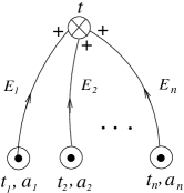
Figure 7: An $n$-point vertex correction arising from uncircled vertices connected to internal circled vertices.

In this case, integrating over the internal time coordinate $t$, leads to

$$\sim\delta(E_{1}+E_{2}+\cdots+E_{n}),$$ (33)

for any given distribution of “thermal” indices. This vanishes at zero temperature. However, under the action of the thermal operator, some of the $E_{i}$’s inside the delta function will change sign and, therefore, the vanishing does not hold for individual graphs. On the other hand, if we sum over the complete set of thermal indices of the internal uncircled vertices, then the contribution is annihilated by the thermal operator as we will show in detail in the following example.

Figure 8: A two loop self-energy insertion in a generic diagram.

Let us consider a typical diagram in $\phi^{3}$ theory with an insertion of the two loop self-energy correction graph as shown in figure (8). In this case, we note that there are two isolated uncircled internal vertices connected among themselves as well as to internal circled vertices (there is no internal uncircled vertex that is connected only to circled vertices). In this case, the contribution of the diagram can be written as

$$\sim\sum_{a_{1},a_{2}}(a_{1})(a_{2})R(a_{1},a_{2})\sum_{a,\tilde{a}}\Gamma_{a\tilde{a}}^{(T=0)},$$ (34)

where we have identified

$$\Gamma_{a\tilde{a}}^{(T=0)}=(a)(\tilde{a})\int dtd\tilde{t}\ \Delta_{a\tilde{a}}^{(T=0)}(t-\tilde{t},E_{5})$$

$$\times\prod_{\alpha=1}^{2}\Delta_{-aa}^{(T=0)}(t_{\alpha}-t,E_{\alpha})\Delta_{-\tilde{a}\tilde{a}}^{(T=0)}(t_{\alpha}-\tilde{t},E_{\alpha+2}).$$ (35)

Using the relation (27), the integration over $t,\tilde{t}$ can be done and for various combinations of the “thermal” indices, the results are

$$\Gamma_{++}^{(T=0)} = -(2\pi i)\left(\prod_{i=1}^{5}\frac{1}{2E_{i}}\right)\delta(E_{1}+E_{2}+E_{3}+E_{4})$$

$$\ \times e^{-i(E_{1}+E_{3})(t_{1}-t_{2})}\left[\frac{1}{E_{3}+E_{4}+E_{5}-i\epsilon}-\frac{1}{E_{3}+E_{4}-E_{5}+i\epsilon}\right],$$

$$\Gamma_{+-}^{(T=0)} = -(2\pi)^{2}\left(\prod_{i=1}^{5}\frac{1}{2E_{i}}\right)\delta(E_{1}+E_{2}-E_{3}-E_{4})$$

$$\ \times e^{-i(E_{1}-E_{3})(t_{1}-t_{2})}\ \delta(E_{3}+E_{4}+E_{5}),$$

$$\Gamma_{-+}^{(T=0)} = -(2\pi)^{2}\left(\prod_{i=1}^{5}\frac{1}{2E_{i}}\right)\delta(E_{1}+E_{2}-E_{3}-E_{4})$$

$$\ \times e^{i(E_{1}-E_{3})(t_{1}-t_{2})}\ \delta(E_{3}+E_{4}+E_{5}),$$

$$\Gamma_{--}^{(T=0)} = (2\pi i)\left(\prod_{i=1}^{5}\frac{1}{2E_{i}}\right)\delta(E_{1}+E_{2}+E_{3}+E_{4})$$ (36)

$$\ \times e^{i(E_{1}+E_{3})(t_{1}-t_{2})}\left[\frac{1}{E_{3}+E_{4}+E_{5}+i\epsilon}-\frac{1}{E_{3}+E_{4}-E_{5}-i\epsilon}\right].$$

It is clear from the structures in (36) that every single component vanishes at zero temperature as a consequence of an energy conserving delta function. We can now apply the thermal operator to these components and explicitly verify that at finite temperature the components no longer vanish individually. On the other hand, if we sum over the “thermal” indices of the internal uncircled vertices (namely, sum over all the components in (36) after applying the thermal operator), then the sum identically vanishes without the use of energy conservation. We have checked this directly, which is tedious, but there is a simpler and more elegant way of seeing this cancellation as follows.

Let us recall (see (7)) that applying the thermal operator simply changes a zero temperature propagator to a finite temperature one. Thus, applying the thermal operator to (35) we can write

$$\Gamma_{++}^{(T)} = \int dtd\tilde{t}\prod_{\alpha=1}^{2}\Delta_{-+}^{(T)}(t_{\alpha}-t,E_{\alpha})\Delta_{-+}^{(T)}(t_{\alpha}-\tilde{t},E_{\alpha+2})\Delta_{++}^{(T)}(t-\tilde{t},E_{5}),$$

$$\Gamma_{+-}^{(T)} = -\int dtd\tilde{t}\prod_{\alpha=1}^{2}\Delta_{-+}^{(T)}(t_{\alpha}-t,E_{\alpha})\Delta_{+-}^{(T)}(t_{\alpha}-\tilde{t},E_{\alpha+2})\Delta_{+-}^{(T)}(t-\tilde{t},E_{5}),$$

$$\Gamma_{-+}^{(T)} = -\int dtd\tilde{t}\prod_{\alpha=1}^{2}\Delta_{+-}^{(T)}(t_{\alpha}-t,E_{\alpha})\Delta_{-+}^{(T)}(t_{\alpha}-\tilde{t},E_{\alpha+2})\Delta_{-+}^{(T)}(t-\tilde{t},E_{5}),$$

$$\Gamma_{--}^{(T)} = \int dtd\tilde{t}\prod_{\alpha=1}^{2}\Delta_{+-}^{(T)}(t_{\alpha}-t,E_{\alpha})\Delta_{+-}^{(T)}(t_{\alpha}-\tilde{t},E_{\alpha+2})\Delta_{--}^{(T)}(t-\tilde{t},E_{5}).$$ (37)

We can now use the KMS condition (4)

$$\Delta_{-+}^{(T)}(t,E) = \Delta_{+-}^{(T)}(t+i\beta,E),$$

$$\Delta_{+-}^{(T)}(t,E) = \Delta_{-+}^{(T)}(t-i\beta,E),$$ (38)

in the first three terms to change all the prefactors to be products of $\Delta_{+-}^{(T)}$ (we also change the last factor in the middle two terms using these relations). Furthermore, since $t,\tilde{t}$ are internal coordinates that are being integrated over, in the first three terms we can make the shifts

$$t\rightarrow t+i\beta,\quad\tilde{t}\rightarrow\tilde{t}+i\beta,$$ (39)

as is necessary to write the sum over the internal thermal indices of the uncircled vertices as

$$\sum_{a,\tilde{a}}\Gamma_{a\tilde{a}}^{(T)} = \int dtd\tilde{t}\prod_{\alpha=1}^{2}\Delta_{+-}^{(T)}(t_{\alpha}-t,E_{\alpha})\Delta_{+-}^{(T)}(t_{\alpha}-\tilde{t},E_{\alpha+2})$$ (40)

$$\quad\times\left(\sum_{a,\tilde{a}}(a)(\tilde{a})\Delta_{a\tilde{a}}^{(T)}(t-\tilde{t},E_{5})\right).$$

The last sum is easily seen to vanish using (28). Thus, we see that even though individual diagrams vanish at zero temperature because of energy conservation, at finite temperature the vanishing holds only when we sum over the thermal indices of the internal uncircled vertices.

In deriving these relations, we have assumed that the internal uncircled vertex or the island of uncircled vertices are connected to internal circled vertices. If any of the circled vertices is external, then our argument does not go through and, in fact, such diagrams would not in general vanish since they are needed to give a cutting description to the diagrams. However, some such diagrams where the internal uncircled vertex is connected to external circled vertex may identically vanish from conservation laws. For example, let us consider the following two loop self-energy diagram in the $\phi^{3}$ theory, shown in figure (9).

Figure 9: A two loop self-energy diagram with an internal uncircled vertex connected to external circled vertices.

In this case, we note that for any value of the thermal index $a$, the integrand has the form

$$\sim R\delta^{3}(k_{1}+k_{2}+k_{3})\prod_{i}\Delta_{a\ -a}(t-t_{i},E_{i})$$ (41)

$$= R\delta^{3}(k_{1}+k_{2}+k_{3})\prod_{i}\frac{e^{i(a)E_{i}(t-t_{i})}}{2E_{i}}$$

When integrated over the internal time coordinate, the result has the form

$$\sim\delta^{3}(k_{1}+k_{2}+k_{3})\delta(E_{1}+E_{2}+E_{3})=0.$$ (42)

As we have noted earlier, the vanishing of this graph follows from the fact that there cannot be a decay involving three on-shell massive particles. This conclusion holds even if one of the $E_{i}$’s changes sign in the delta function and so the vanishing of these individual graphs continues to hold at finite temperature (as can be easily seen from the action of the thermal operator).

Thus, we see that in this doubled theory at zero temperature, when the internal “thermal” indices are summed, the nontrivial graphs contributing to the imaginary part in the momentum space consist of diagrams where there are regions of circled and uncircled vertices connected to the external vertices in a continuous manner such that a cutting description holds. Furthermore, through the application of the thermal operator (since every propagator factors into the same thermal operator that is independent of time), it follows that a cutting description of the graphs holds even at finite temperature in a completely parallel manner. The cutting rules for this theory at finite temperature and $\mu=0$ are already well known. However, this gives a simpler derivation of the cutting description through the application of the thermal operator.

II.1 Example

As an example of the cutting description through the thermal operator, let us calculate the imaginary part of the one loop retarded self-energy at finite temperature for the $\phi^{3}$ theory. This imaginary part has been calculated from various points of view. Here we merely give a brief derivation of this to illustrate the application of the thermal operator representation.

In the case of the self-energy, Eq. (18) graphically takes the form shown in figure (10).

Figure 10: Graphical representation of Eq. (17) for a one loop self-energy diagram.

Furthermore, if we are interested only in the retarded self-energy, the second diagram with the circled vertex on the right can be shown to add up to zero. Consequently, the nontrivial diagram that would contribute to the imaginary part of the retarded self-energy at one loop has the form shown in figure (11).

Figure 11: The one loop self-energy graph leading to the imaginary part.

Ignoring the momentum integration, (namely, $\int\frac{d^{3}k_{1}d^{3}k_{2}}{(2\pi)^{6}}\ (2\pi)^{3}\delta^{3}(k_{1}+k_{2}-p)$), the diagram leads to

$$-i\overline{\Pi}_{ab}^{(T=0)} = \frac{(-ig)(ig)(a)(b)}{2}\prod_{i=1}^{2}\Delta_{-b\ b}(t_{1}-t_{2},E_{i})$$ (43)

$$= \frac{(a)(b)g^{2}}{2}\frac{1}{4E_{1}E_{2}}\ e^{-i(b)(E_{1}+E_{2})(t_{1}-t_{2})},$$

where we have used the compact representation of the propagators in (27) as well as the fact that the two point function is identified with $-i\overline{\Pi}$ where $\overline{\Pi}$ denotes the appropriate self-energy. Since the retarded self-energy at zero temperature is given by

$$\Pi_{\rm R}^{(T=0)}=\Pi_{++}^{(T=0)}+\Pi_{+-}^{(T=0)},$$ (44)

using (43) and taking the Fourier transform with respect to the time coordinate, we obtain the imaginary part of the retarded self-energy in momentum space to be

$${\rm Im}\Pi_{\rm R}^{(T=0)}(p)=-\frac{1}{2}(-i\overline{\Pi}_{\rm R}^{(T=0)}(p)=\frac{i}{2}\overline{\Pi}_{\rm R}^{(T=0)}(p)$$ (45)

$$= -\frac{1}{2}\int dt\frac{g^{2}}{8E_{1}E_{2}}\left(e^{i(p_{0}-E_{1}-E_{2})t}-e^{i(p_{0}+E_{1}+E_{2})t}\right)$$

$$= \!\!-\frac{(2\pi)g^{2}}{16E_{1}E_{2}}\left(\delta(p_{0}-E_{1}-E_{2})-\delta(p_{0}+E_{1}+E_{2})\right).$$

Applying the relevant thermal operator for the graph silvana1 ; Brandt:2006rv

$${\cal O}^{(T)}=\prod_{i=1}^{2}\left(1+n(E_{i})(1-S(E_{i}))\right),$$ (46)

we obtain the imaginary part of the retarded self energy at one loop at finite temperature to be

$${\rm Im}\Pi_{\rm R}^{(T)}(p)$$ (47)

$$= -\frac{(2\pi)g^{2}}{16E_{1}E_{2}}\Big{[}(1+n(E_{1})+n(E_{2}))$$

$$\quad\times(\delta(p_{0}-E_{1}-E_{2})-\delta(p_{0}+E_{1}+E_{2}))$$

$$\quad+(n(E_{1})-n(E_{2}))$$

$$\quad\times(\delta(p_{0}+E_{1}-E_{2})-\delta(p_{0}-E_{1}+E_{2}))\big{]},$$

which is well known in the literature.

III Cutting Rules at Finite Temperature and $\mu\neq 0$

The cutting rules at finite temperature in the absence of a chemical potential are well known in the closed time path formalism. In the earlier section, we have given a simple derivation of these rules through the application of the thermal operator on the cutting description of a zero temperature theory with doubled degrees of freedom. In this section we will derive the cutting rules for a theory at finite temperature with a nonzero chemical potential through the application of the thermal operator (which we have also verified directly) and to the best of our knowledge, this has not been done in the closed time path formalism. As we will see, the proof of a cutting description in this case will be quite parallel to that discussed in the last section. Therefore, instead of repeating arguments, we will give only the essential details in this section.

Let us consider for simplicity a toy model of an interacting theory of a real and a complex scalar field described by the Lagrangian density

$${\cal L} = \frac{1}{2}\partial_{\mu}\sigma\partial^{\mu}\sigma-\frac{m^{2}}{2}\sigma^{2}+\left((\partial_{t}-i\mu)\phi\right)^{*}(\partial_{t}-i\mu)\phi$$ (48)

$$\quad-(\vec{\nabla}\phi)^{*}\cdot\vec{\nabla}\phi-M^{2}\phi^{*}\phi-g\sigma\phi^{*}\phi,$$

where $\mu$ stands for the chemical potential of the complex scalar field and is assumed to have a value $\mu<M$. For the real scalar field, there is no chemical potential and the components of the thermal propagator in the closed time path formalism factorize through a thermal operator as discussed in Eqs. (7, 8). For the complex scalar field with a chemical potential, however, the components of the propagator in the closed time path formalism are more complicated. In the momentum space, they can be written as

$$G_{++}^{(T,\mu)}(p) = \frac{i}{(p_{0}+\mu)^{2}-E^{2}+i\epsilon}$$

$$\quad+2\pi n^{(\mu)}(p_{0})\delta((p_{0}+\mu)^{2}-E^{2}),$$

$$G_{+-}^{(T,\mu)}(p) = 2\pi\left(\theta(-p_{0}-\mu)+n^{(\mu)}(p_{0})\right)$$

$$\quad\times\delta((p_{0}+\mu)^{2}-E^{2}),$$

$$G_{-+}^{(T,\mu)}(p) = 2\pi\left(\theta(p_{0}+\mu)+n^{(\mu)}(p_{0})\right)$$

$$\quad\times\delta((p_{o}+\mu)^{2}-E^{2}),$$

$$G_{--}^{(T,\mu)}(p) = -\frac{i}{(p_{0}+\mu)^{2}-E^{2}-i\epsilon}$$ (49)

$$\quad+2\pi n^{(\mu)}(p_{0})\delta((p_{0}+\mu)^{2}-E^{2}),$$

where

$$E=\sqrt{\vec{p}^{\ 2}+M^{2}},\quad n^{(\mu)}(p_{0})=n(p_{0}{\rm sgn}(p_{0}+\mu)).$$ (50)

In the mixed space, they take the forms silvana1

$$G_{++}^{(T,\mu)}(t,E) = \frac{1}{2E}\left((\theta(t)+n_{-}(E))e^{-iE_{-}t}\right.$$

$$\qquad\left.+(\theta(-t)+n_{+}(E))e^{iE_{+}t}\right),$$

$$G_{+-}^{(T,\mu)}(t,E) = \frac{1}{2E}\left(n_{-}(E)e^{-iE_{-}t}+(1+n_{+}(E))e^{iE_{+}t}\right),$$

$$G_{-+}^{(T,\mu)}(t,E) = \frac{1}{2E}\left((1+n_{-})e^{-iE_{-}t}+n_{+}(E)e^{iE_{+}t}\right),$$

$$G_{--}^{(T,\mu)}(t,E) = \frac{1}{2E}\left((\theta(t)+n_{+}(E))e^{iE_{+}t}\right.$$ (51)

$$\qquad\left.+(\theta(-t)+n_{-})e^{-iE_{-}t}\right),$$

where we have defined

$$E_{\pm}=E\pm\mu,\quad n_{\mp}(E)=n(E\mp\mu)=\frac{1}{e^{\beta(E\mp\mu)}-1}.$$ (52)

In the zero temperature limit, the components of the propagator take the form

$$G_{++}^{(T=0,\mu)}(t,E) = \frac{1}{2E}\left(\theta(t)e^{-iE_{-}t}+\theta(-t)e^{iE_{+}t}\right),$$

$$G_{+-}^{(T=0,\mu)}(t,E) = \frac{1}{2E}\ e^{iE_{+}t},$$

$$G_{-+}^{(T=0,\mu)}(t,E) = \frac{1}{2E}\ e^{-iE_{-}t},$$

$$G_{--}^{(T=0,\mu)}(t,E) = \frac{1}{2E}\left(\theta(t)e^{iE_{+}t}+\theta(-t)e^{-iE_{-}t}\right).$$ (53)

As is clear from (51), in the presence of a chemical potential, the components of the thermal propagator are more complicated mainly because the distribution function for the positive and the negative frequency terms in the propagator are different. In this case, a simple factorization as in (7,8) in terms of the simple reflection operator $S(E)$ alone does not work. Rather, a time independent factorization of the propagator and, therefore, a thermal representation for any finite temperature graph can be obtained if we introduce an additional operator $\hat{N}^{(T,\mu)}(E)$ such that

$$\hat{N}^{(T,\mu)}(E)f(E_{\mp})=n_{\mp}(E)f(E_{\mp}).$$ (54)

In this case, we can write the components of the thermal propagator in a factorized manner as

$$G_{ab}^{(T,\mu)}(t,E)={\cal O}^{(T,\mu)}(E)G_{ab}^{(T=0,\mu)}(E),$$ (55)

where

$${\cal O}^{(T,\mu)}(E)=1+\hat{N}^{(T,\mu)}(E)(1-S(E)).$$ (56)

The action of this additional operator has already been discussed in Inui:2006jf ; Brandt:2006vy to which we refer the readers for more details.

Given the mixed space propagators of the zero temperature theory with doubled degrees of freedom, one look at their positive and negative frequency decomposition as in (9). This leads to the set of circled propagators as in (10) both at zero as well as finite temperatures. (We give the spectral representation for the components of the propagator at finite temperature in appendix B.) It is easy to see from the definition of the circled propagators that the set of circled propagators at finite temperature factorize into that at zero temperature and the thermal operator (56), namely,

$$G_{ab}^{(T,\mu)}(t_{1}-t_{2},E) = {\cal O}^{(T,\mu)}(E)G_{ab}^{(T=0,\mu)}(t_{1}-t_{2},E),$$

$$G_{ab}^{(T,\mu)}(t_{1}-\underline{t_{2}},E) = {\cal O}^{(T,\mu)}(E)G_{ab}^{(T=0,\mu)}(t_{1}-\underline{t_{2}},E),$$

$$G_{ab}^{(T,\mu)}(\underline{t_{1}}-t_{2},E) = {\cal O}^{(T,\mu)}(E)G_{ab}^{(T=0,\mu)}(\underline{t_{1}}-t_{2},E),$$

$$G_{ab}^{(T,\mu)}(\underline{t_{1}}-\underline{t_{2}},E) = {\cal O}^{(T,\mu)}(E)G_{ab}^{(T=0,\mu)}(\underline{t_{1}}-\underline{t_{2}},E).$$

We note here that the propagator where both ends are circled corresponds to the anti time ordered propagator which can be easily seen to be the complex conjugate of the original propagator in the momentum space. (It is interesting to point out here that in the presence of the chemical potential, the doubly circled propagator is not the complex conjugate even for the “$\pm\pm$” components in the mixed space unlike the case when $\mu=0$.) We can also introduce the circled vertices as in (11) in this theory.

From the definition of the set of circled propagators, identities such as (13,LABEL:lte1) can be easily seen to hold in the presence of a chemical potential and, therefore, it follows that the largest time equation (see (15)) also holds in this case. Through the application of the thermal operator, the largest time equation also holds at finite temperature in the presence of a chemical potential. Namely, if we add to a graph with the largest time coordinate uncircled, a corresponding graph with the largest time coordinate circled, the sum identically vanishes. Incidentally, since identities such as (13,LABEL:lte1) can be checked directly to hold for the components of the propagator at finite temperature with $\mu\neq 0$, the largest time equation can also be checked to hold directly (independent of the proof through the application of the thermal operator). From the largest time equation, it then follows that the diagrams still satisfy the identity (18) so that the imaginary part of a diagram in momentum space can be given a diagrammatic representation.

To obtain a cutting description, we proceed as in the last section. First, it can be checked as in the case of $\mu=0$ that there are only two basic independent components of the propagator, namely, $G_{+-}^{(T=0,\mu)},G_{-+}^{(T=0,\mu)}$ such that we can express all the components of the propagators including the circled ones as ($a,b=\pm$)

$$G_{ab}^{(T=0,\mu)}(t_{1}-\underline{t_{2}},E) = G_{a\ -a}^{(T=0,\mu)}(t_{1}-t_{2},E),$$

$$G_{ab}^{(T=0,\mu)}(\underline{t_{1}}-t_{2},E) = G_{-b\ b}^{(T=0,\mu)}(t_{1}-t_{2},E),$$

$$G_{ab}^{(T=0,\mu)}(t_{1}-t_{2},E) = \theta(t_{1}-t_{2})G_{-b\ b}^{(T=0,\mu)}(t_{1}-t_{2},E)$$

$$+ \theta(t_{2}-t_{1})G_{a\ -a}^{(T=0,\mu)}(t_{1}-t_{2},E),$$

$$G_{ab}^{(T=0,\mu)}(\underline{t_{1}}-\underline{t_{2}},E) = \theta(t_{1}-t_{2})G_{a\ -a}^{(T=0,\mu)}(t_{1}-t_{2},E)$$

$$+ \theta(t_{2}-t_{1})G_{-b\ b}^{(T=0,\mu)}(t_{1}-t_{2},E).$$

From this relation it follows that much like (28), for any circling of the time coordinates $t_{1},t_{2}$, we have

$$\sum_{a,b=\pm}(a)(b)G_{ab}^{(T=0,\mu)}(t_{1}-t_{2},E)=0.$$ (59)

Let us also note for completeness that the basic components of the propagator $G_{\pm\mp}^{(T=0,\mu)}$ can be written in a compact form (see (27)) as

$$G_{a\ -a}^{(T=0,\mu)}(t_{1}-t_{2},E)=\frac{1}{2E}e^{i(a)E_{(a)}(t_{1}-t_{2})}.$$ (60)

Since all the basic identities one needs to prove a cutting description of the imaginary part of a diagram (in the momentum space) in the case $\mu=0$ also hold for $\mu\neq 0$, we can go through the discussions of the last section. However, without repeating the arguments, we simply conclude that in the presence of a chemical potential, a cutting description for the imaginary part of a graph holds in the zero temperature theory with doubled degrees of freedom, when summed over the “thermal” indices of the internal vertices in a graph. Through the application of the thermal operator, we then conclude that such a description also holds at finite temperature with $\mu\neq 0$. We note here that independent of the thermal operator argument, one can directly verify that all the relevant identities hold for the components of the propagator at finite temperature and $\mu\neq 0$ so that one can also prove a cutting description for any graph at finite temperature directly (which we have done). However, the power of the thermal operator representation is that once the cutting description is shown to hold at zero temperature in the theory with a doubled degrees of freedom, it automatically holds at finite temperature.

III.1 Example

As an application of the cutting rules in the presence of a chemical potential, let us again calculate the imaginary part of the self-energy for the real scalar particle at one loop in this theory. Let us note that in the mixed space, the two point function shown in figure (12) has a very simple form (we follow the same notation as in (43))

Figure 12: One loop diagram leading to the imaginary part of the self energy. The dashed lines represent the neutral scalar field and the solid lines the complex scalar field with the arrow representing the direction of the charge flow.

$$-i\overline{\Pi}_{ab}^{(T=0,\mu)}$$ (61)

$$= \frac{g^{2}(a)(b)}{2}G_{b\ -b}^{(T=0,\mu)}(t_{2}-t_{1},E_{1})G_{-b\ b}^{(T=0,\mu)}(t_{1}-t_{2},E_{2})$$

$$= \frac{g^{2}(a)(b)}{8E_{1}E_{2}}e^{-i(b)(E_{1(b)}+E_{2(-b)})(t_{1}-t_{2})},$$

where we have used the representation given in (60). Since the retarded self-energy is defined as (see (44))

$$\Pi_{\rm R}^{(T=0,\mu)}=\Pi_{++}^{(T=0,\mu)}+\Pi_{+-}^{(T=0,\mu)},$$ (62)

we obtain from (61)

$$-i\overline{\Pi}_{\rm R}^{(T=0,\mu)}(t_{1}-t_{2})$$

$$= \frac{g^{2}}{8E_{1}E_{2}}\left(e^{-i(E_{1+}+E_{2-})(t_{1}-t_{2})}-e^{i(E_{1-}+E_{2+})(t_{1}-t_{2})}\right).$$

Taking the Fourier transform of this, we obtain the imaginary part of the retarded self-energy to be (as in the earlier example, we are ignoring the momentum integration and the factors associated with them, namely, $\int\frac{d^{3}k_{1}d^{3}k_{2}}{(2\pi)^{6}}(2\pi)^{3}\delta^{3}(k_{1}+k_{2}-p)$)

$${\rm Im}\Pi_{\rm R}^{(T=0,\mu)}(p)=\frac{i}{2}\overline{\Pi}_{\rm R}^{(T=0,\mu)}(p)=-\frac{(2\pi)g^{2}}{16E_{1}E_{2}}$$ (64)

$$\times\left(\delta(p_{0}-E_{1+}-E_{2-})-\delta(p_{0}+E_{1-}+E_{2+})\right).$$

We note that the chemical potential in a loop cancels out completely which is also reflected in the fact that if we are to substitute the expressions for $E_{i\pm}$ inside the delta functions, there will be no $\mu$ dependence in the retarded self-energy. This is, in fact, the correct result and is what we should do if we are interested in the imaginary part of the retarded self-energy at zero temperature. However, as explained in Inui:2006jf ; Brandt:2006vy , to obtain the temperature dependent terms through the application of the thermal operator in (56) using the relation (54), we should use the explicit expressions for $E_{i\pm}$ only after the application of the thermal operator. Using the thermal operator, we obtain the imaginary part of the retarded self-energy to be

$${\rm Im}\Pi_{\rm R}^{(T,\mu)}(p)={\cal O}^{(T,\mu)}(E_{1}){\cal O}^{(T,\mu)}(E_{2}){\rm Im}\Pi_{\rm R}^{(T=0,\mu)}(p)$$ (65)

$$= -\frac{(2\pi)g^{2}}{16E_{1}E_{2}}\big{[}(1+n_{+}(E_{1})+n_{-}(E_{2}))\delta(p_{0}-E_{1}-E_{2})$$

$$\quad-(1+n_{-}(E_{1})+n_{+}(E_{2}))\delta(p_{0}+E_{1}+E_{2})$$

$$\quad-(n_{+}(E_{1})-n_{+}(E_{2}))\delta(p_{0}-E_{1}+E_{2})$$

$$\quad+(n_{-}(E_{1})-n_{-}(E_{2}))\delta(p_{0}+E_{1}-E_{2})\big{]}.$$

This is easily seen to reduce to (47) when $\mu=0$ and has all the symmetry properties of a retarded self-energy.

We would like to point out here that with the use of the circled propagators and vertices, one can not only calculate the imaginary part of the retarded self-energy, but also the complete retarded self-energy as well as the appropriate dispersion relation at any temperature (including zero temperature). Let us note using the largest time equation (analogous to (LABEL:lte1) for the self-energy) that

$$\theta(t_{1}-t_{2})\left(\Pi_{ab}^{(T=0,\mu)}(t_{1}-t_{2})+\Pi_{ab}^{(T=0,\mu)}(\underline{t_{1}}-t_{2})\right)=0,$$ (66)

which can also be represented graphically as

$$\theta(t_{1}-t_{2})\left[\begin{array}[]{c}\includegraphics[scale={0.4}]{cf8.eps}\end{array}\right]=0.$$ (67)

From the definition of the retarded self-energy in (62) as well as the fact that the retarded self-energy (by definition) is proportional to $\theta(t_{1}-t_{2})$, it follows that

$$\Pi_{\rm R}^{(T=0,\mu)}(t_{1}-t_{2})=\theta(t_{1}-t_{2})\Pi_{\rm R}^{(T=0,\mu)}(t_{1}-t_{2})$$ (68)

$$= \theta(t_{1}-t_{2})\left(\Pi_{++}^{(T=0,\mu)}(t_{1}-t_{2})+\Pi_{+-}^{(T=0,\mu)}(t_{1}-t_{2})\right)$$

$$= -\theta(t_{1}-t_{2})\left(\Pi_{++}^{(T=0,\mu)}(\underline{t_{1}}-t_{2})+\Pi_{+-}^{(T=0,\mu)}(\underline{t_{1}}-t_{2})\right)$$

$$= -\theta(t_{1}-t_{2})\overline{\Pi}_{\rm R}^{(T=0,\mu)}(t_{1}-t_{2}).$$

Here we have used (66) in the intermediate step and have identified the appropriate graphs with $(-i\overline{\Pi}^{(T=0,\mu)})$ defined earlier. We recall that the Fourier transform of $(-i\overline{\Pi})$ is related to the imaginary part of the retarded self-energy in momentum space (see (45) or (64)). Therefore, (68) gives a method for calculating the complete retarded self-energy using the circled propagators and vertices at zero temperature which can then be extended to finite temperature through the application of the thermal operator. In fact, using the integral representation for the theta function,

$$\theta(t_{1}-t_{2})=\frac{1}{2\pi i}\int dq_{0}\ \frac{e^{iq_{0}(t_{1}-t_{2})}}{q_{0}-i\epsilon},$$ (69)

and taking the Fourier transform of (68), we obtain

$$\Pi_{\rm R}^{(T=0,\mu)}(p) = -\frac{1}{2\pi i}\int dq_{0}\ \frac{\overline{\Pi}_{\rm R}^{(T=0,\mu)}(q_{0}+p_{0},\vec{p})}{q_{0}-i\epsilon}$$ (70)

$$= \frac{1}{\pi}\int dq_{0}\ \frac{{\rm Im}\Pi_{\rm R}^{(T=0,\mu)}(q_{0}+p_{0},\vec{p})}{q_{0}-i\epsilon}.$$

This, therefore, leads to the dispersion relation for the retarded self-energy at zero temperature and through the application of the thermal operator, it follows that the dispersion relation holds even at finite temperature, namely,

$$\Pi_{\rm R}^{(T,\mu)}(p)=\frac{1}{\pi}\int dq_{0}\ \frac{{\rm Im}\Pi_{\rm R}^{(T,\mu)}(q_{0}+p_{0},\vec{p})}{q_{0}-i\epsilon}.$$ (71)

Using the imaginary part of the retarded self-energy from (65) and carrying out the delta function integrations, we obtain the complete one loop retarded self-energy in momentum space at finite temperature and chemical potential to be (of course, we must still perform the momentum integrations alluded to earlier)

$$\Pi_{\rm R}^{(T,\mu)}(p) = -\frac{g^{2}}{8E_{1}E_{2}}\left[\frac{1+n_{+}(E_{1})+n_{-}(E_{2})}{E_{1}+E_{2}-p_{0}-i\epsilon}\right.$$ (72)

$$\quad+\frac{1+n_{-}(E_{1})+n_{+}(E_{2})}{E_{1}+E_{2}+p_{0}+i\epsilon}$$

$$\quad-\frac{n_{+}(E_{1})-n_{+}(E_{2})}{E_{1}-E_{2}-p_{0}-i\epsilon}$$

$$\quad\left.-\frac{n_{-}(E_{1})-n_{-}(E_{2})}{E_{1}-E_{2}+p_{0}+i\epsilon}\right].$$

This expression is exact and can be used to compute $\Pi_{\rm R}^{(T,\mu)}(p)$ in various limits of physical interest.

IV Summary

In this paper, we have systematically studied the interesting question of cutting rules at finite temperature as an application of the thermal operator representation. The thermal operator relates in a direct manner the finite temperature graphs to those of the zero temperature theory. Thus, we have studied first a zero temperature scalar theory with doubled degrees of freedom (that can be obtained from the zero temperature limit of the finite temperature theory in the closed time path formalism). We have given an alternative algebraic derivation of the largest time equation for this theory. We have derived the cutting description at zero temperature and then through the action of the thermal operator we have shown that the cutting description also holds at finite temperature and zero/finite chemical potential. As an example, we have calculated the imaginary part of the one loop retarded self-energy at finite temperature and zero/finite chemical potential. We have also shown how the circled propagators and vertices can be used to obtain the dispersion relation as well as the full retarded self-energy of thermal particles.

Acknowledgement

This work was supported in part by the US DOE Grant number DE-FG 02-91ER40685, by MCT/CNPq as well as by FAPESP, Brazil and by CONICYT, Chile under grant Fondecyt 1030363 and 7040057 (Int. Coop.).

Appendix A Derivation of Identities for the Largest Time Equation

In this appendix, we give a brief derivation of the identity used in (15) with a generalization to theories with $n$-point interactions. Let us consider expressions consisting of products of $n$-factors of the forms

$$I_{n} = \prod_{i=1}^{n}A_{i}-\prod_{i=1}^{n}B_{i},$$

$$\tilde{I}_{n} = \prod_{i=1}^{n}A_{i}+\prod_{i=1}^{n}B_{i},$$ (73)

where $A_{i},B_{i}$ are arbitrary. It follows from this that

$$\prod_{i=1}^{n}A_{i}=\frac{1}{2}(I_{n}+\tilde{I}_{n}),\quad\prod_{i=1}^{n}B_{i}=\frac{1}{2}(-I_{n}+\tilde{I}_{n}).$$ (74)

It follows from this that

$$I_{n+1} = A_{n+1}\prod_{i=1}^{n}A_{i}-B_{n+1}\prod_{i=1}^{n}B_{i}$$

$$= \frac{1}{2}(A_{n+1}+B_{n+1})I_{n}+\frac{1}{2}(A_{n+1}-B_{n+1})\tilde{I}_{n},$$

$$\tilde{I}_{n+1} = A_{n+1}\prod_{i=1}^{n}A_{i}+B_{n+1}\prod_{i=1}^{n}B_{i}$$ (75)

$$= \frac{1}{2}(A_{n+1}-B_{n+1})I_{n}+\frac{1}{2}(A_{n+1}+B_{n+1})\tilde{I}_{n}.$$

These relations can be written in a matrix form as

$$\left(\begin{array}[]{c}I_{n+1}\\ \tilde{I}_{n+1}\end{array}\right)=\frac{1}{2}\left(\begin{array}[]{cc}A_{n+1}+B_{n+1}&A_{n+1}-B_{n+1}\\ &\\ A_{n+1}-B_{n+1}&A_{n+1}+B_{n+1}\end{array}\right)\left(\begin{array}[]{c}I_{n}\\ \tilde{I}_{n}\end{array}\right).$$ (76)

Iterating this, we obtain (we only note the forms of $I_{n}$ which are relevant for our discussion)

$$I_{1} = A_{1}-B_{1},$$

$$I_{2} = \frac{1}{2}\left[(A_{1}-B_{1})(A_{2}+B_{2})+(A_{2}-B_{2})(A_{1}+B_{1})\right],$$

$$I_{3} = \frac{1}{4}\left[(A_{1}-B_{1})(A_{2}+B_{2})(A_{3}+B_{3})\right.$$ (77)

$$\quad+(A_{2}-B_{2})(A_{3}+B_{3})(A_{1}+B_{1})$$

$$\quad+(A_{3}-B_{3})(A_{1}+B_{1})(A_{2}+B_{2})$$

$$\quad\left.+(A_{1}-B_{1})(A_{2}-B_{2})(A_{3}-B_{3})\right],$$

and so on. Identifying

$$A_{i} = \theta(t-t_{i})\Delta_{aa_{i}}^{(T=0)}(t-t_{i},E_{i}),$$

$$B_{i} = \theta(t-t_{i})\Delta_{aa_{i}}^{(T=0)}(\underline{t}-t_{i},E_{i}),$$ (78)

the identity in (15) follows. If we had a theory with an $n$-point interaction, we can iterate the above relation $n$ times to obtain the particular identity. The important thing to note is that in this difference of products, there will always be a factor of the form $(A-B)$ in every term and with the identification in (78), such a factor will always vanish because of (LABEL:lte1). As a result, the largest time equation holds for any theory.

Appendix B Spectral Representation for the Propagator at Finite Temperature and $\mu\neq 0$

In our discussions in this paper, we have worked in a mixed space representation for the propagator and, as a result, we have been able to read out the positive and the negative frequency components of the propagator directly from the definition in (9). However, when one works in the momentum space, there is no time coordinate and, therefore, no direct notion of time ordering. In this case, the positive and the negative frequency components of a propagator are obtained from a spectral decomposition of the propagator. In this appendix, we describe briefly the spectral decomposition for a scalar propagator at finite temperature in the presence of a chemical potential. The corresponding analysis for $\mu=0$ was already discussed in das:book97 and can be obtained from this discussion in the limit of a vanishing chemical potential.

Let us note that since the components of the propagator at finite temperature depend on both positive and negative frequency components, one can write a general spectral decomposition for the propagator as

$$G_{ab}^{(T,\mu)}(x) = \int\frac{d^{4}p}{(2\pi)^{4}}\ G_{ab}^{(T,\mu)}(p)\ e^{-ip\cdot x}$$ (79)

$$= i\int_{0}^{\infty}\!\!\!ds\int\frac{d^{4}p}{(2\pi)^{4}}\!\left[\frac{\rho_{ab}^{(T,\mu)}(s,p)}{(p_{0}+\mu)^{2}-\vec{p}^{\ 2}-s+i\epsilon}\right.$$

$$\quad\left.+\frac{\tilde{\rho}_{ab}^{(T,\mu)}(s,p)}{(p_{0}+\mu)^{2}-\vec{p}^{\ 2}-s-i\epsilon}\right]e^{-ip\cdot x}.$$

From the structure of the components of the momentum space propagator in (49), we can read out the spectral functions in (79) to be

$$\rho_{++}^{(T,\mu)}(s,p) = (1+n^{(\mu)}(p_{0}))\delta(s-M^{2})=-\tilde{\rho}_{--}^{(T,\mu)}(s,p),$$

$$\rho_{+-}^{(T,\mu)}(s,p) = \left(\theta(-p_{0}-\mu)+n^{(\mu)}(p_{0})\right)\delta(s-M^{2})$$

$$= -\tilde{\rho}_{+-}^{(T,\mu)}(s,p),$$

$$\rho_{-+}^{(T,\mu)}(s,p) = \left(\theta(p_{0}+\mu)+n^{(\mu)}(p_{0})\right)\delta(s-M^{2})$$

$$= -\tilde{\rho}_{-+}^{(T,\mu)}(s,p),$$

$$\rho_{--}^{(T,\mu)}(s,p) = n^{(\mu)}(p_{0})\delta(s-M^{2})=-\tilde{\rho}_{++}^{(T,\mu)}(s,p).$$ (80)

We note that when $\mu=0$, these reduce to the spectral functions already described in das:book97 . For $T=0$, the spectral functions are given by

$$\rho_{++}^{(T=0,\mu)}(s,p) = \delta(s-M^{2})=-\tilde{\rho}_{--}^{(T=0,\mu)}(s,p),$$

$$\rho_{+-}^{(T=0,\mu)}(s,p) = \theta(-p_{0}-\mu)\delta(s-M^{2})=-\tilde{\rho}_{+-}^{(T=0,\mu)}(s,p),$$

$$\rho_{-+}^{(T=0,\mu)}(s,p) = \theta(p_{0}+\mu)\delta(s-M^{2})=-\tilde{\rho}_{-+}^{(T=0,\mu)}(s,p),$$

$$\rho_{--}^{(T=0,\mu)}(s,p) = 0=\tilde{\rho}_{++}^{(T=0,\mu)}(s,p).$$ (81)

The components of the propagator are time ordered and carrying out the integration in (79) over the $p_{0}$ variable would, in fact, show this and lead to the frequency decomposition

$$G_{ab}^{(T,\mu)}(x)=\theta(x^{0})G_{ab}^{(T,\mu)(+)}(x)+\theta(-x^{0})G_{ab}^{(T,\mu)(-)}(x).$$ (82)

In fact, comparing with (79), we can now determine

$$G_{ab}^{(T,\mu)(\pm)}(x)$$

$$= \int_{0}^{\infty}ds\int\frac{d^{4}p}{(2\pi)^{4}}\ (2\pi)\delta((p_{0}+\mu)^{2}-\vec{p}^{\ 2}-s)\ e^{-ip\cdot x}$$

$$\times \left[\theta(\pm(p_{0}+\mu))\rho_{ab}^{(T,\mu)}(s,p)-\theta(\mp(p_{0}+\mu))\tilde{\rho}_{ab}^{(T,\mu)}(s,p)\right].$$

The positive and the negative frequency components in the mixed space can be related to the spectral functions as

$$G_{ab}^{(T,\mu)\pm}(t,E)$$

$$= \int_{0}^{\infty}ds\int dp_{0}\ \delta((p_{0}+\mu)^{2}-E^{2}-s+M^{2})e^{-ip_{0}t}$$

$$\times \left[\theta(\pm(p_{0}+\mu))\rho_{ab}^{(T,\mu)}(s,p)-\theta(\mp(p_{0}+\mu))\tilde{\rho}_{ab}^{(T,\mu)}(s,p)\right].$$

Recalling that all the spectral functions in (80) are proportional to $\delta(s-M^{2})$ and that the remaining factor depends only on $p_{0}$, let us define

$$\rho_{ab}^{(T,\mu)}(s,p) = \delta(s-M^{2})\rho_{ab}^{(T,\mu)}(p_{0}),$$

$$\tilde{\rho}_{ab}^{(T,\mu)}(s,p) = \delta(s-M^{2})\tilde{\rho}_{ab}^{(T,\mu)}(p_{0}).$$ (85)

Then, the positive and the negative frequency components in the mixed space can also be written as (doing the $s$ integration)

$$G_{ab}^{(T,\mu)\pm}(t,E)=\int dp_{0}\delta((p_{0}+\mu)^{2}-E^{2})\ e^{-ip_{0}t}$$

$$\times\left[\theta(\pm(p_{0}+\mu))\rho_{ab}^{(T,\mu)}(p_{0})-\theta(\mp(p_{0}+\mu))\tilde{\rho}_{ab}^{(T,\mu)}(p_{0})\right],$$

which are the expressions used in the text (although we have derived these directly from the expressions of the components of the propagators in the mixed space).

References

• (1) H. A. Weldon, Phys. Rev. D 28, 2007 (1983).
• (2) S. Jeon, Phys. Rev. D 47, 4586 (1993); ibid D 52, 3591 (1995).
• (3) R. L. Kobes and G. Semenoff, Nucl. Phys. B 260, 714 (1985); ibid B 272, 329 (1986).
• (4) N. Ashida, H. Nakagawa and A. Niegawa, Ann. of Phys. 215, 315 (1992).
• (5) N. Ashida, H. Nakagawa, A. Niegawa and H. Yokota, Phys. Rev. D 45, 2066 (1992).
• (6) P. F. Bedaque, A. K. Das and S. Naik, Mod. Phys. Lett. A 12, 2481 (1997).
• (7) A. Das, Finite Temperature Field Theory (World Scientific, NY, 1997).
• (8) P. V. Landshoff, Phys. Lett. B 386, 291 (1996).
• (9) R. J. Cutkosky, J. Math. Phys. 1, 429 (1960).
• (10) G. ’t Hooft and M. Veltman, “Diagrammar,” (1974) CERN-73-09.
• (11) O. Espinosa and E. Stockmeyer, Phys. Rev. D69, 065004 (2004).
• (12) O. Espinosa, Phys. Rev. D71, 065009 (2005).
• (13) F. T. Brandt, A. Das, O. Espinosa, J. Frenkel and S. Perez, Phys. Rev. D 72, 085006 (2005).
• (14) F. T. Brandt, A. Das, O. Espinosa, J. Frenkel and S. Perez, Phys. Rev. D 73, 065010 (2006).
• (15) J. I. Kapusta, Finite Temperature Field Theory (Cambridge University Press, Cambridge, England, 1989);
• (16) M. L. Bellac, Thermal Field Theory (Cambridge University Press, Cambridge, England, 1996).
• (17) M. Inui, H. Kohyama and A. Niegawa, Phys. Rev. D 73, 047702 (2006).
• (18) F. T. Brandt, A. Das, O. Espinosa, J. Frenkel and S. Perez, Phys. Rev. D 73, 067702 (2006).
• (19) R. Kubo, J. Phys. Soc. Japan, 12, 570 (1957).
• (20) P. C. Martin and J. Schwinger, Phys. Rev. 115, 1342 (1959).