Abstract

By taking the freezing limit of a spin Calogero-Sutherland model containing ‘anyon like’ representation of the permutation algebra, we derive the exact partition function of $SU(m|n)$ supersymmetric Haldane-Shastry (HS) spin chain. This partition function allows us to study global properties of the spectrum like level density distribution and nearest neighbour spacing distribution. It is found that, for supersymmetric HS spin chains with large number of lattice sites, continuous part of the energy level density obeys Gaussian distribution with a high degree of accuracy. The mean value and standard deviation of such Gaussian distribution can be calculated exactly. We also conjecture that the partition function of supersymmetric HS spin chain satisfies a duality relation under the exchange of bosonic and fermionic spin degrees of freedom.

PACS No. : 02.30.Ik, 75.10.Jm, 05.30.-d, 03.65.Fd

Keywords : Haldane-Shastry spin chain, partition function, level density distribution, supersymmetry

1 Introduction

Haldane-Shastry (HS) spin chain is a well known quantum integrable model, where equally spaced spins on a circle interact with each other through pairwise exchange interactions inversely proportional to the square of their chord distances. Study of such HS spin-$\frac{1}{2}$ chain with long-range interaction was originally motivated from the fact that the exact ground state wavefunction of this model coincides with the $U\rightarrow\infty$ limit of Gutzwiller’s variational wave function for the Hubbard model, and also with the one-dimensional version of the resonating valence bond state proposed by Anderson [1,2]. Remarkably, HS spin chain can be explicitly solved in much greater detail than integrable spin chains with short-range interactions, has a Yangian quantum group symmetry and interestingly shares many of the characteristics of an ideal gas, but with fractional statistics [3-5]. The Hamiltonian of $SU(m)$ HS model with $N$ number of lattice sites is given by

$$H=\frac{1}{2}\sum_{1\leq j<k\leq N}\frac{(1+P_{jk})}{\sin^{2}(\xi_{j}-\xi_{k})}\,,$$ (1.1)

where $\xi_{j}=j\pi/N$ and $P_{jk}$ is the exchange operator interchanging the ‘spins’ (taking $m$ possible values) on $j$-th and $k$-th lattice sites.

By using the motif representations associated with $Y(gl_{m})$ Yangian symmetry of HS spin chain (1.1), one can find out its complete spectrum including the degeneracy factor for each energy level [6-8]. However, in practice, the computation of such degeneracy factors becomes very cumbersome for $m>2$ and large values of $N$. Therefore, it is difficult to express the partition function of HS spin chain in a simple form (for arbitrary values of $N$ and $m$) with the help of motif representations. Due to this reason, it is worthwhile to explore other approaches for calculating the partition function of HS spin chain. In fact, a rather simple expression for the exact partition function of $SU(m)$ HS spin chain has been obtained recently [9] by applying the so called freezing trick [10-12]. This freezing trick utilizes the connection between $SU(m)$ HS spin Hamiltonian and $SU(m)$ spin Calogero-Sutherland (CS) model which has dynamical as well as spin degrees of freedom. More precisely, one takes the strong coupling limit of spin CS Hamiltonian, so that the particles freeze at their classical equilibrium positions of the scalar part of the potential and spins get decoupled from the dynamical degree of freedom. As a result, one can derive the partition function of HS spin chain by ‘modding out’ the partition function of spinless CS model from that of the spin CS model. By using this partition function of $SU(m)$ HS spin chain, it is possible to study the energy level density distribution and the nearest neighbour spacing distribution for fairly large values of $N$ [9]. Interestingly, it has been found that, the continuous part of such energy level density follows Gaussian distribution to a high degree of approximation.

In this context it may be noted that, there exists a $SU(m|n)$ supersymmetric extension of HS spin chain [3], where each site is occupied by either one of the $m$ type of bosonic states or one of the $n$ type of fermionic states. Such supersymmetric spin chains play an important role in describing some correlated systems of condensed matter physics, where holes moving in the dynamical background of spin behave as bosons and spin-$\frac{1}{2}$ electrons behave as fermions [13]. It is worth noting that the supersymmetric $SU(m|n)$ HS spin chain exhibits $Y(gl_{(m|n)})$ super-Yangian symmetry [3], which is also the quantum group symmetry of supersymmetric $SU(m|n)$ Polychronakos spin chain [14,15]. Consequently, by using the motif representations and skew-Young diagrammes associated with supersymmetric Polychronakos spin chain [15], one can in principle calculate the degeneracy factors for all energy eigenvalues of supersymmetric HS spin chain. However, similar to the nonsupersymmetric case, this method for finding the full spectrum and related partition function becomes very complicated for large values of $N$.

The aim of the present article is to find out the exact partition function for supersymmetric $SU(m|n)$ HS model by applying the freezing trick and also to study global properties like level density distribution of the corresponding spectrum. For this purpose, it is convenient to map the supersymmetric HS model to a usual spin chain containing an ‘anyon like’ representation of the permutation algebra as spin dependent interactions [16,17]. In Sec.2 we describe this mapping and also show how the freezing trick can be applied for the case of $SU(m|n)$ HS spin chain by embedding it in a spin CS model containing the same anyon like representation of the permutation algebra. In Sec.3, we find out the complete spectrum of such spin CS model including the degeneracy factors for all energy levels. In Sec.4, we calculate the partition function of this spin CS model at the strong coupling limit and divide it by that of the spinless CS model to finally obtain the partition function of $SU(m|n)$ HS spin chain. In this section, we also discuss about the motif representation for $SU(m|n)$ HS spin chain and find that, due to the lifting of a selection rule, some extra energy levels appear in the spectrum in comparison with the case of $SU(m)$ spin chain. Subsequently, we conjecture that the partition function of $SU(m|n)$ HS model satisfies a duality relation under the exchange of bosonic and fermionic spin degrees of freedom. In Sec.5, we study the level density distribution and the nearest neighbour spacing distribution for the spectrum of $SU(m|n)$ HS spin chain by using its exact partition function. It is found that, for sufficiently large values of $N$, continuous part of the energy level density satisfies the Gaussian distribution with a high degree of accuracy. We also derive exact expressions for the mean value and standard deviation which characterize such Gaussian distribution. Sec.6 is the concluding section.

2 Application of the freezing trick

For the purpose of defining the $SU(m|n)$ supersymmetric HS spin chain, let us consider a set of operators like $C_{j\alpha}^{\dagger}$($C_{j\alpha}$) which creates (annihilates) a particle of species $\alpha$ on the $j$-th lattice site. These creation (annihilation) operators are assumed to be bosonic when $\alpha\in[1,2,....,m]$ and fermionic when $\alpha\in[m+1,m+2,....,m+n]$. Thus, the parity of $C_{j\alpha}^{\dagger}$($C_{j\alpha}$) is defined as

$$p(C_{j\alpha})=p(C_{j\alpha}^{\dagger})=0~{}\mathnormal{for}~{}\alpha\in[1,2,....,m]\,,$$

$$p(C_{j\alpha})=p(C_{j\alpha}^{\dagger})=1~{}\mathnormal{for}~{}\alpha\in[m+1,m+2,....,m+n]\,.$$

These operators satisfy commutation (anti-commutation) relations like

$$[C_{j\alpha},C_{k\beta}]_{\pm}=0\,,~{}[C_{j\alpha}^{\dagger},C_{k\beta}^{\dagger}]_{\pm}=0\,,~{}[C_{j\alpha},C_{k\beta}^{\dagger}]_{\pm}=\delta_{jk}\delta_{\alpha\beta}\,,$$ (2.1)

where $[A,B]_{\pm}\equiv AB-(-1)^{p(A)p(B)}BA$. Next, we focus our attention to a subspace of the related Fock space, for which the total number of particles per site is always one:

$$\sum_{\alpha=1}^{m+n}C_{j\alpha}^{\dagger}C_{j\alpha}=1,$$ (2.2)

for all $j$. On the above mentioned subspace, one can define supersymmetric exchange operators as

$$\hat{P}_{jk}^{(m|n)}\equiv\sum_{\alpha,\beta=1}^{m+n}C_{j\alpha}^{\dagger}C_{k\beta}^{\dagger}C_{j\beta}C_{k\alpha}\,,$$ (2.3)

where $1\leq j<k\leq N$. These $\hat{P}_{jk}^{(m|n)}$’s yield a realization of the permutation algebra given by

$$\mathcal{P}_{jk}^{2}=1\,,~{}\mathcal{P}_{jk}\mathcal{P}_{kl}=\mathcal{P}_{jl}\mathcal{P}_{jk}=\mathcal{P}_{kl}\mathcal{P}_{jl}\,,~{}[\mathcal{P}_{jk},\mathcal{P}_{lm}]=0\,,$$ (2.4)

where $j,~{}k,~{}l,~{}m$ are all distinct indices. Replacing $P_{jk}$ by $\hat{P}_{jk}^{(m|n)}$ in eqn.(1.1), one obtains the Hamiltonian of $SU(m|n)$ supersymmetric HS model as [3]

$$\mathcal{H}^{(m|n)}=\frac{1}{2}\sum_{1\leq j<k\leq N}\frac{\left(1+\hat{P}_{jk}^{(m|n)}\right)}{\sin^{2}(\xi_{j}-\xi_{k})}.$$ (2.5)

Now we want to describe how this $SU(m|n)$ supersymmetric HS model (2.5), containing creation-annihilation operators, can be transformed to a spin chain. To this end, we consider a particular type of anyon like representation of permutation algebra (2.4), which acts on a spin state like $|\alpha_{1}\alpha_{2}\dots\alpha_{N}\rangle$ (with $\alpha_{j}\in[1,2,\dots,m+n]$) as [16,17]

$$\tilde{P}_{jk}^{(m|n)}|\alpha_{1}\dots\alpha_{j}\dots\alpha_{k}\dots\alpha_{N}\rangle=e^{i\Phi(\alpha_{j},\alpha_{j+1},\dots,\alpha_{k})}|\alpha_{1}\dots\alpha_{k}\dots\alpha_{j}\dots\alpha_{N}\rangle,$$ (2.6)

where $e^{i\Phi(\alpha_{j},\alpha_{j+1},\dots,\alpha_{k})}=1$ if $\alpha_{j},\alpha_{k}\in[1,2,\dots,m]$, $e^{i\Phi(\alpha_{j},\alpha_{j+1},\dots,\alpha_{k})}=-1$ if $\alpha_{j},\alpha_{k}\in[m+1,m+2,\dots,m+n]$, and $e^{i\Phi(\alpha_{j},\alpha_{j+1},\dots,\alpha_{k})}=(-1)^{{\pi\sum_{p=j+1}^{k-1}\sum_{\tau=m+1}^{m+n}\delta_{\alpha_{p},\tau}}}$ if $\alpha_{j}\in[1,2,\dots,m]$ and $\alpha_{k}\in[m+1,m+2,\dots,m+n]$ or vice versa. For the purpose of interpreting the phase factor $e^{i\Phi(\alpha_{j},\alpha_{j+1},\dots,\alpha_{k})}$ in a physical way, it is convenient to call $\alpha_{i}$ a ‘bosonic’ spin when $\alpha_{i}\in[1,2,\dots,m]$ and a ‘fermionic’ spin when $\alpha_{i}\in[m+1,m+2,\dots,m+n]$. From eqn.(2.6) it follows that, the exchange of two bosonic (fermionic) spins produces a phase factor of $1\,(-1)$ irrespective of the nature of spins situated in between the $j$-th and $k$-th lattice sites. However, if we exchange one bosonic spin with one fermionic spin, then the phase factor becomes $(-1)^{\rho}$ where $\rho$ is the total number of fermionic spins situated in between the $j$-th and $k$-th lattice sites.

Next we observe that, due to the constraint (2.2), the Hilbert space associated with $SU(m|n)$ HS Hamiltonian (2.5) can be spanned through the following orthonormal basis vectors: $C_{1\alpha_{1}}^{\dagger}C_{2\alpha_{2}}^{\dagger}\dots C_{N\alpha_{N}}^{\dagger}|0\rangle$, where $|0\rangle$ is the vacuum state and $\alpha_{j}\in[1,2,\dots,m+n]$. Consequently, it is possible to define a one-to-one mapping between these basis vectors and those of the above mentioned spin chain as

$$|\alpha_{1}\alpha_{2}\dots\alpha_{N}\rangle\leftrightarrow C_{1\alpha_{1}}^{\dagger}C_{2\alpha_{2}}^{\dagger}\dots C_{N\alpha_{N}}^{\dagger}|0\rangle.$$ (2.7)

With the help of commutation (anti-commutation) relations (2.1), one can easily verify that

$$\hat{P}_{jk}^{(m|n)}\,C_{1\alpha_{1}}^{\dagger}\dots C_{j\alpha_{j}}^{\dagger}\dots C_{k\alpha_{k}}^{\dagger}\dots C_{N\alpha_{N}}^{\dagger}|0\rangle$$

$$~{}~{}~{}~{}~{}~{}~{}~{}~{}~{}~{}~{}~{}~{}~{}~{}~{}~{}~{}~{}~{}~{}~{}~{}~{}~{}\,=\,e^{i\Phi(\alpha_{j},\dots,\alpha_{k})}\,C_{1\alpha_{1}}^{\dagger}\dots C_{j\alpha_{k}}^{\dagger}\dots C_{k\alpha_{j}}^{\dagger}\dots C_{N\alpha_{N}}^{\dagger}|0\rangle,~{}~{}~{}~{}$$ (2.8)

where $e^{i\Phi(\alpha_{j},\dots,\alpha_{k})}$ is the same phase factor which appeared in eqn.(2.6). Comparison of eqn.(2.8) with eqn.(2.6) through the mapping (2.7) reveals that, the anyon like representation $\tilde{P}_{jk}^{(m|n)}$ is equivalent to the supersymmetric exchange operator $\hat{P}_{jk}^{(m|n)}$. Hence, if we define a spin chain Hamiltonian through $\tilde{P}_{jk}^{(m|n)}$ as

$$H^{(m|n)}=\frac{1}{2}\sum_{1\leq j<k\leq N}\frac{\left(1+\tilde{P}_{jk}^{(m|n)}\right)}{\sin^{2}(\xi_{j}-\xi_{k})},$$ (2.9)

that would be completely equivalent to the supersymmetric $SU(m|n)$ HS model (2.5) [16]. Clearly, for the special case $n=0$, $\tilde{P}_{jk}^{(m|n)}$ reproduces the original spin exchange operator $P_{jk}$ and ${H}^{(m|n)}$ (2.9) reduces to the Hamiltonian of $SU(m)$ HS spin chain (1.1). Since it is convenient to apply the freezing trick to the spin chain Hamiltonian (2.9), for the rest of this article we shall deal with this form of supersymmetric $SU(m|n)$ HS model instead of its original form (2.5).

By using the anyon like representation $\tilde{P}_{jk}^{(m|n)}$, one can construct a spin CS model like

$$H^{*}=-\sum_{j=1}^{N}\frac{\partial^{2}}{\partial x_{j}^{2}}+2a\sum_{1\leq j<k\leq N}\frac{\big{(}\,a+\tilde{P}_{jk}^{(m|n)}\,\big{)}}{\sin^{2}(x_{j}-x_{k})}\,,$$ (2.10)

which contains spin as well as dynamical degrees of freedom and the positive parameter $a$ as coupling constant. With the help of mapping (2.7) it can be shown that, this spin CS model is equivalent to a supersymmetric spin CS model [18] with $Y(gl_{(m|n)})$ super-Yangian symmetry. The spin CS Hamiltonian $H^{*}$ (2.10) might be formally written as

$$H^{*}=H_{0}+4a\mathsf{H}^{(m|n)},$$ (2.11)

where $H_{0}$ is the Hamiltonian of spinless CS model given by [19]

$$H_{0}=-\sum_{j=1}^{N}\frac{\partial^{2}}{\partial x_{j}^{2}}+2a(a-1)\sum_{1\leq j<k\leq N}\frac{1}{\sin^{2}(x_{j}-x_{k})}\,,$$ (2.12)

and $\mathsf{H}^{(m|n)}$ is obtained from $H^{(m|n)}$ (2.9) by the replacement $\xi_{j}\rightarrow x_{j}$. Now the decoupling of the dynamical degrees of freedom of $H^{*}$ (2.10) from its spin degrees of freedom can be achieved by using the freezing trick [10-12]. This trick is based on the fact that in the limit $a\rightarrow\infty$, particles freeze at the equilibrium positions of $H_{0}$, which are simply the lattice points ($\xi_{j}$) of the spin chain in eqn.(2.9). Consequently, by using eqn.(2.11) at freezing limit, we find that the energy levels of $H^{*}$ are approximately given by

$$E^{*}_{jk}\simeq E_{0,j}+4aE_{k},$$ (2.13)

where $E_{0,j}$ and $E_{k}$ are any two levels of $H_{0}$ and $H^{(m|n)}$ respectively. Hence, we obtain a relation like

$$Z^{(m|n)}(T)=\lim_{a\rightarrow\infty}\frac{Z^{*}(4aT)}{Z_{0}(4aT)},$$ (2.14)

where $Z^{(m|n)}$, $Z^{*}$ and $Z_{0}$ denote the partition functions corresponding to the Hamiltonians $H^{(m|n)}$, $H^{*}$ and $H_{0}$ respectively. Thus the freezing trick allows us to compute the partition function of $SU(m|n)$ supersymmetric HS spin chain, by modding out the contribution of spinless CS model from the partition function of spin CS model (2.10). Due to the Gallelian invariance of $H^{*}$ and $H_{0}$ it follows that, if $\psi$ is an eigenstate of any one of these Hamiltonians with momentum $p$, then $\psi^{\prime}=e^{2i\tau\sum_{j=1}^{N}x_{j}}\psi$ will also be an eigenstate of the same Hamiltonian with momentum $(p+2\tau N)$. As a result, we can always adjust the parameter $\tau$ such that $\psi^{\prime}$ will be an eigenfunction of $H^{*}$ or $H_{0}$ with zero momentum. In this article, we shall always consider eigenstates of these Hamiltonians with zero momenta and evaluate the partition functions $Z^{*}$ as well as $Z_{0}$ at the center of mass frame. Since both $Z^{*}$ and $Z_{0}$ get modified by the same multiplicative factor due to a Gallelian transformation, $Z^{(m|n)}$ does not depend on the choice of the reference frame.

3 Spectrum of spin CS model

In this section our aim is to find out the complete spectrum of spin CS model (2.10) containing anyon like representation of the permutation algebra. Even though the spectrum of such spin CS model has been studied earlier [17], multiplicities of degenerate eigenfunctions corresponding to all energy levels have not been found. Since these numbers are required for calculating the partition function of this model, here we want to derive a general expression for the degeneracy factors of all energy levels. It is well known that the eigenfunctions of spin CS Hamiltonian (2.10) can be written in a factorised form like

$$\psi(x_{1},\dots,x_{N};\alpha_{1},\dots,\alpha_{N})=\Gamma^{a}\phi(x_{1},\dots,x_{N};\alpha_{1},\dots,\alpha_{2}),$$ (3.1)

where $\Gamma=\prod_{i<j}\sin(x_{i}-x_{j})$. By operating $H^{*}$ (2.10) on the above form of $\psi$, we find that

$$H^{*}\psi=\Gamma^{a}\tilde{H}^{*}\phi,$$ (3.2)

where

$$\tilde{H}^{*}=4\biggl{[}\sum_{j}\biggl{(}z_{j}\frac{\partial}{\partial z_{j}}\biggr{)}^{2}+a\sum_{k<j}\frac{z_{k}+z_{j}}{z_{k}-z_{j}}\biggl{(}z_{k}\frac{\partial}{\partial z_{k}}-z_{j}\frac{\partial}{\partial z_{j}}\biggr{)}~{}~{}~{}~{}~{}~{}~{}~{}~{}~{}$$

$$~{}~{}~{}~{}~{}~{}~{}~{}-2a\sum_{k<j}(1+\tilde{P}^{(m|n)}_{jk})\frac{z_{j}z_{k}}{(z_{j}-z_{k})^{2}}+\frac{a^{2}}{12}N(N^{2}-1)\biggr{]},$$ (3.3)

with $z_{j}=e^{2ix_{j}}$. Equation (3.2) implies that, if $\phi$ is an eigenvector of $\tilde{H}^{*}$ with eigenvalue $E$, then $\Gamma^{a}\phi$ would be an eigenvector of $H^{*}$ with the same eigenvalue. Thus the diagonalisation problem of $H^{*}$ is reduced to the diagonalisation problem of $\tilde{H}^{*}$.

For solving $\tilde{H}^{*}$, it is convenient to introduce another operator $\mathcal{H}$ which acts only on the coordinate degree of freedom and may be given by [7]

$$\mathcal{H}=4\biggl{[}\sum_{j}\biggl{(}z_{j}\frac{\partial}{\partial z_{j}}\biggr{)}^{2}+a\sum_{k<j}\frac{z_{k}+z_{j}}{z_{k}-z_{j}}\biggl{(}z_{k}\frac{\partial}{\partial z_{k}}-z_{j}\frac{\partial}{\partial z_{j}}\biggr{)}~{}~{}~{}~{}~{}~{}~{}~{}~{}~{}$$

$$~{}~{}~{}~{}~{}~{}~{}~{}-2a\sum_{k<j}(1-K_{jk})\frac{z_{j}z_{k}}{(z_{j}-z_{k})^{2}}+\frac{a^{2}}{12}N(N^{2}-1)\biggr{]},$$ (3.4)

where the $K_{jk}$ is the coordinate exchange operator which exchanges the coordinates of $j$-th and $k$-th particle:

$$K_{jk}f(x_{1},\dots,x_{j},\dots,x_{k},\dots,x_{N})=f(x_{1},\dots,x_{k},\dots,x_{j},\dots,x_{N}).$$

It may be observed that, $\tilde{H}^{*}$ (3.3) can be reproduced from the expression of $\mathcal{H}$ (3.4) through the substitution $K_{jk}\rightarrow-\tilde{P}_{jk}^{(m|n)}$. This connection between $\tilde{H}^{*}$ and $\mathcal{H}$ will play a crucial role in our calculation for finding the spectrum of $\tilde{H}^{*}$. Let us first consider state vectors given by monomials like

$$\xi_{\bf{p}}=z_{1}^{p_{1}}z_{2}^{p_{2}}\dots z_{N}^{p_{N}},$$ (3.5)

where ${\bf p}\equiv\{p_{1},p_{2},\dots,p_{N}\}\in\mathbb{R}^{N}$ satisfies the constraints: (i) $(p_{i}-p_{j})$ are integers for all $i,j$ and (ii) $\sum_{i=1}^{N}p_{i}=0$. The last condition implies that these monomials represent state vectors with zero total momentum. In particular, one can consider $\xi_{\bf\hat{p}}$ corresponding to a nonincreasing vector ${\bf\hat{p}}\equiv(\hat{p}_{1},\hat{p}_{2},\dots,\hat{p}_{N})$, whose elements satisfy the conditions: (i) $l_{i}\equiv\hat{p}_{i}-\hat{p}_{i+1}$ is a nonnegative integer for $i\in[1,\dots,N-1]$ and (ii) $\sum_{i=1}^{N}{\hat{p}}_{i}=0$. It is evident that, $N-1$ number of nonnegative integers ($l_{i}$’s) are sufficient to specify a nonincreasing vector ${\bf\hat{p}}$. Given two distinct nonincreasing vectors ${\bf\hat{p}}$ and ${\bf\hat{p}^{\prime}}$, we shall write ${\bf\hat{p}}\prec{\bf\hat{p}^{\prime}}$ if $\hat{p}_{1}-\hat{p}_{1}^{\prime}=\dots=\hat{p}_{i-1}-\hat{p}_{i-1}^{\prime}=0$ and $\hat{p}_{i}<\hat{p}_{i}^{\prime}$. A partial ordering can be defined on monomials like $\xi_{\bf{p}}$ (3.5) in the following way. By permuting the elements of any ${\bf p}$, one can always construct a unique nonincreasing vector ${\bf\hat{p}}$. The basis element $\xi_{\bf p}$ would precede $\xi_{\bf p^{\prime}}$ if ${\bf\hat{p}}\prec{\bf\hat{p}^{\prime}}$, where ${\bf\hat{p}}$ and ${\bf\hat{p}^{\prime}}$ are nonincreasing vectors obtained from ${\bf p}$ and ${\bf p^{\prime}}$ respectively by permuting their components. The above defined ordering is effectively a partial ordering, since it does not induce an ordering between $\xi_{\bf p}$ and $\xi_{\bf p^{\prime}}$ when ${\bf\hat{p}}={\bf\hat{p}^{\prime}}$. It can be shown that the action of $\mathcal{H}$ (3.4) on the state vector $\xi_{\bf p}$ yields [7,9]

$$\mathcal{H}\xi_{\bf p}\,=\,E_{\bf\hat{p}}\xi_{\bf p}+\sum_{\begin{subarray}{c}{\bf p^{\prime}}\\ ({\bf\hat{p}^{\prime}}<{\bf\hat{p}})\end{subarray}}c_{{\bf p}{\bf p^{\prime}}}\xi_{\bf p^{\prime}}\,,$$ (3.6)

where

$$E_{\bf\hat{p}}=\sum_{i=1}^{N}\left\{2\hat{p_{i}}+a(N+1-2i)\right\}^{2}.$$ (3.7)

Thus it is clear that, if one constructs a Hilbert space through basis vectors of the form (3.5) and partially order them in the above mentioned way, then $\mathcal{H}$ will act as a triangular matrix on this space.

Next we want to construct another partially ordered Hilbert space, on which $\tilde{H}^{*}$ (3.3) can be represented as a triangular matrix. To this end, we define a set of permutation operators as $\Pi_{jk}^{(m|n)}=\tilde{P}_{jk}^{(m|n)}K_{jk}$. Since both $\tilde{P}_{jk}^{(m|n)}$ and $K_{jk}$ satisfy an algebra of the form (2.4), while acting on the spin and coordinate spaces respectively, the newly defined operator $\Pi_{jk}^{(m|n)}$ also yields a representation of the same permutation algebra on the direct product of coordinate and spin spaces. Hence, by using this representation of permutation algebra, we can construct a ‘generalized’ antisymmetric projection operator $\Lambda^{(m|n)}$ satisfying the relation

$$\Pi_{jk}^{(m|n)}\Lambda^{(m|n)}=\Lambda^{(m|n)}\Pi_{jk}^{(m|n)}=-\Lambda^{(m|n)}\,,$$ (3.8)

or, equivalently, $\tilde{P}_{jk}^{(m|n)}\Lambda^{(m|n)}=-K_{jk}\Lambda^{(m|n)}$ [16,17]. Even though $\Lambda^{(m|n)}$ can be expressed as a function of $\Pi_{jk}^{(m|n)}$, explicit form of this projection operator is not necessary for our present purpose. However it may be noted that, since both $K_{jk}$ and $\tilde{P}_{jk}^{(m|n)}$ commute with $\mathcal{H}$ (3.4), $\Lambda^{(m|n)}$ also satisfies the relation

$$[\mathcal{H},\Lambda^{(m|n)}]=0\,.$$ (3.9)

With the help of projection operator $\Lambda^{(m|n)}$, we define a state vector on the direct product of coordinate and spin spaces as

$$\phi^{\boldsymbol{\alpha}}_{\bf p}\equiv\phi^{\alpha_{1}\dots\alpha_{N}}_{p_{1}\dots p_{N}}=\Lambda^{(m|n)}\{\xi_{\bf p}|\alpha_{1}\dots\alpha_{N}\rangle\}.$$ (3.10)

Using eqns.(3.8) and (2.6) it can be shown that

$$\phi^{\alpha_{1}\dots\alpha_{j}\dots\alpha_{k}\dots\alpha_{N}}_{p_{1}\dots\,p_{j}\dots\,p_{k}\dots\,p_{N}}\hskip-15.93347pt =-\Lambda^{(m|n)}K_{jk}{\tilde{P}}_{jk}^{(m|n)}\{z_{1}^{p_{1}}\dots z_{j}^{p_{j}}\dots z_{k}^{p_{k}}\dots z_{N}^{p_{N}}|\alpha_{1}\dots\alpha_{j}\dots\alpha_{k}\dots\alpha_{N}\rangle\}$$ (3.11)

$$=-e^{i\Phi(\alpha_{j},\dots,\alpha_{k})}\Lambda^{(m|n)}\{z_{1}^{p_{1}}\dots z_{j}^{p_{k}}\dots z_{k}^{p_{j}}\dots z_{N}^{p_{N}}|\alpha_{1}\dots\alpha_{k}\dots\alpha_{j}\dots\alpha_{N}\rangle\}$$

$$=-e^{i\Phi(\alpha_{j},\dots,\alpha_{k})}\phi^{\alpha_{1}\dots\alpha_{k}\dots\alpha_{j}\dots\alpha_{N}}_{p_{1}\dots\,p_{k}\dots\,p_{j}\dots\,p_{N}}\,.$$

By repeatedly using the above equation we find that

$$\phi_{\bf p}^{\boldsymbol{\alpha}}=\epsilon({\boldsymbol{\alpha}},{\bf p})\,\phi_{\bf\hat{p}}^{\boldsymbol{\alpha^{\prime}}},$$ (3.12)

where $\epsilon({\boldsymbol{\alpha}},{\bf p})=\pm 1$, ${\bf\hat{p}}$ is the nonincreasing vector corresponding to ${\bf p}$ and ${\boldsymbol{\alpha^{\prime}}}$ is a spin vector which is obtained by permuting the components of ${\boldsymbol{\alpha}}$. Hence, all state vectors of the form (3.10) can be obtained by choosing ${\bf p}$ from the set of nonincreasing vectors only.

Corresponding to any given nonincreasing vector ${\bf\hat{p}}$, one can define a vector space as

$$\mathbb{V}_{\bf\hat{p}}\equiv\langle\,\phi_{\bf\hat{p}}^{\boldsymbol{\alpha}}~{}~{}|\,\alpha_{1},\dots,\alpha_{N}\in[1,2,\dots m+n]\,\rangle\,.$$ (3.13)

It is important to note that, different values of ${\boldsymbol{\alpha}}$ may lead to the same $\phi_{\bf\hat{p}}^{\boldsymbol{\alpha}}$ which is a basis element of $\mathbb{V}_{\bf\hat{p}}$. To see this thing in a simple way, let us take a nonincreasing sequence ${\bf\hat{p}}$ satisfying the condition $\hat{p}_{i}=\hat{p}_{j}=\hat{p}$ (say). For this special case, eqn.(3.11) reduces to

$$\phi^{\alpha_{1}\dots\alpha_{i}\dots\alpha_{j}\dots\alpha_{N}}_{\,\hat{p}_{1}\,\dots\,\hat{p}\,\dots\,\hat{p}\,\dots\,\hat{p}_{N}}=-\,e^{i\Phi(\alpha_{i},\dots,\alpha_{j})}\,\phi^{\alpha_{1}\dots\alpha_{j}\dots\alpha_{i}\dots\alpha_{N}}_{\,\hat{p}_{1}\,\dots\,\hat{p}\,\dots\,\hat{p}\,\dots\,\hat{p}_{N}}\,.$$ (3.14)

Clearly $\phi^{\alpha_{1}\dots\alpha_{i}\dots\alpha_{j}\dots\alpha_{N}}_{\,\hat{p}_{1}\,\dots\,\hat{p}\,\dots\,\hat{p}\,\dots\,\hat{p}_{N}}$ and $\phi^{\alpha_{1}\dots\alpha_{j}\dots\alpha_{i}\dots\alpha_{N}}_{\,\hat{p}_{1}\,\dots\,\hat{p}\,\dots\,\hat{p}\,\dots\,\hat{p}_{N}}$ represent the same state vector (up to a phase factor), although they correspond to different values of ${\boldsymbol{\alpha}}$. For a given $\phi_{\bf\hat{p}}^{\boldsymbol{\alpha}}$, we say that two spin components of ${\boldsymbol{\alpha}}$ belong to the same ‘sector’ if the corresponding two components of ${\bf\hat{p}}$ are equal to each other. For example, the spin components $\alpha_{i}$ and $\alpha_{j}$ appearing in the state $\phi^{\alpha_{1}\dots\alpha_{i}\dots\alpha_{j}\dots\alpha_{N}}_{\,\hat{p}_{1}\,\dots\,\hat{p}\,\dots\,\hat{p}\,\dots\,\hat{p}_{N}}$ belong to the same sector according to this convention. Since $e^{i\Phi}=1$, for $\alpha_{i},\alpha_{j}\in[1,2,\dots,m]$, it is clear from eqn.(3.14) that bosonic spins within the same sector obey ‘fermionic statistics’ after antisymmetrisation. In particular, two bosonic spins of same flavour can not coexist within a single sector. Similarly, since $e^{i\Phi}=-1$ for $\alpha_{i},\alpha_{j}\in[m+1,m+2,\dots,m+n]$, one can find from eqn.(3.14) that fermionic spins within the same sector obey ‘bosonic statistics’ after antisymmetrisation. Therefore, any number of fermionic spins having the same flavour can be accommodated within a single sector.

Now we want to find out the dimensionality of the space $\mathbb{V}_{\bf\hat{p}}$. For this purpose, it is useful to write ${\bf\hat{p}}$ in the form

$$\bf{\hat{p}}\equiv\big{(}\overbrace{\rho_{1},\dots,\rho_{1}}^{k_{1}},\dots,\overbrace{\rho_{i},\dots,\rho_{i}}^{k_{i}},\dots,\overbrace{\rho_{r},\dots,\rho_{r}}^{k_{r}}\big{)},$$ (3.15)

where $\rho_{1}>\dots>\rho_{i}>\dots>\rho_{r}$, $\sum_{i=1}^{r}k_{i}=N$, and $r$ is an integer which can take any value from $1$ to $N$. It is obvious that ${\bf k}\equiv\{k_{1},\dots,k_{r}\}$, which belongs to the set $\mathcal{P}_{N}$ of ordered partitions of $N$, may be treated as a function of $\bf{\hat{p}}$. For a given $\phi_{\bf\hat{p}}^{\boldsymbol{\alpha}}$, clearly the components of $\boldsymbol{\alpha}$ are separated into $r$ different sectors where the $i$-th sector contains $k_{i}$ number of spins. It is evident that the dimensionality of the space $\mathbb{V}_{\bf\hat{p}}$ may be obtained by counting the number of independent ways one can distribute total $N$ number of spins within $r$ sectors. To this end, let us first try to find out the number of independent ways of filling up the $i$-th sector through $j_{1}$ number of bosonic spins and $j_{2}$ number of fermionic spins, where $j_{1}+j_{2}=k_{i}$. Using eqn.(3.14) we have already seen that, bosonic and fermionic spins within the same sector obey fermionic and bosonic statistics respectively. Therefore, we can pick up $j_{1}$ number of bosonic spins from $m$ different flavours in ${}^{m}C_{j_{1}}$ different ways and $j_{2}$ number of fermionic spins from $n$ different flavours in ${}^{j_{2}+n-1}C_{j_{2}}$ ways, where ${}^{p}C_{l}=\frac{p\,!}{l\hskip 0.28436pt!\,(p-l)!}$ for $l\leq p$ and ${}^{p}C_{l}=0$ for $l>p$. Thus the number of independent ways of filling up the $i$-th sector through $j_{1}$ number of bosonic spins and $j_{2}$ number of fermionic spins is given by

$${}^{m}C_{j_{1}}\,^{n+j_{2}-1}C_{j_{2}}\,.$$

Summing up these numbers for all possible values of $j_{1}$ and $j_{2}$, we obtain the total number of independent ways of filling up the $i$-th sector through $k_{i}$ number of spins as

$$d^{(m|n)}(k_{i}) = \sum_{j_{1}=~{}0}^{k_{i}}\big{(}\,^{m}C_{j_{1}}\,^{n+k_{i}-j_{1}-1}C_{k_{i}-j_{1}}\,\big{)}$$ (3.16)

$$= \sum_{j_{1}=~{}0}^{{\rm min}\,(m,k_{i})}\frac{m!~{}(n+k_{i}-j_{1}-1)!}{j_{1}!~{}(m-j_{1})!~{}(n-1)!~{}(k_{i}-j_{1})!}\,.$$

Since two spins belonging to different sectors do not follow any exchange relation like (3.14), the number of independent ways we can distribute total $N$ number of spins within $r$ different sectors is given by the product of all $d^{(m|n)}(k_{i})$. Therefore, by using (3.16), we finally obtain the dimension of $\mathbb{V}_{\bf\hat{p}}$ as

$$d^{(m|n)}({\bf k})=\prod_{i=1}^{r}d^{(m|n)}(k_{i})=\prod_{i=1}^{r}\left(\sum_{j=0}^{{\rm min}\,(m,k_{i})}\,{}^{m}C_{j}\,{}^{n+k_{i}-j-1}C_{k_{i}-j}\right)\,.$$ (3.17)

Even though this expression is derived by assuming that bosonic and fermionic spin degrees of freedom (i.e., $m$ and $n$ respectively) take nonzero values, it is also possible to obtain the dimension of $\mathbb{V}_{\bf\hat{p}}$ for the $SU(n)$ fermionic case by putting $m=0$ in eqn.(3.17):

$$d^{(0|n)}({\bf k})=\prod_{i=1}^{r}~{}^{n+k_{i}-1}C_{k_{i}}\,.$$ (3.18)

Furthermore, by putting $n=0$ in eqn.(3.17), subsequently using the relation ${}^{p}C_{l}=0$ for $l>p\geq 0$, and also assuming that ${}^{-1}C_{0}=1$, one can reproduce the dimension of $\mathbb{V}_{\bf\hat{p}}$ for the $SU(m)$ bosonic case [9] as

$$d^{(m|0)}({\bf k})=\prod_{i=1}^{r}~{}^{m}C_{k_{i}}.$$ (3.19)

It is interesting to observe that, while $d^{(m|0)}({\bf k})$ (3.19) can take a nonzero value only if $k_{i}\leq m$ for all $i$, both $d^{(m|n)}({\bf k})$ (3.17) and $d^{(0|n)}({\bf k})$ (3.18) take nonzero values for any ${\bf k}\in\mathcal{P}_{N}$. Consequently, $\mathbb{V}_{\bf\hat{p}}$ will represent a nontrivial vector space for the $SU(m)$ bosonic case only if at most $m$ components of ${\bf\hat{p}}$ take the same value. On the other hand, $\mathbb{V}_{\bf\hat{p}}$ will represent a nontrivial vector space for all possible values of ${\bf\hat{p}}$ when at least one fermionic spin degrees of freedom is present.

The Hilbert space associated with $\tilde{H}^{*}$ (3.3) may now be defined by taking the direct sum of $\mathbb{V}_{\bf\hat{p}}$ (3.13) for all allowed values of ${\bf\hat{p}}\,$:

$$\mathbb{V}=\mathop{\oplus}_{\bf\hat{p}}\mathbb{V}_{\bf\hat{p}}\,.$$ (3.20)

We define a partial ordering in this Hilbert space by saying that the basis element $\phi_{\bf\hat{p}}^{\boldsymbol{\alpha}}$ precedes $\phi_{\bf\hat{p^{\prime}}}^{\boldsymbol{\alpha^{\prime}}}$ if ${\bf\hat{p}}\prec{\bf\hat{p}^{\prime}}$. By consecutively applying the relations (3.10), (3.8), (3.9), (3.6) and (3.12), it is easy to check that

$$\tilde{H}^{*}(\phi^{\boldsymbol{\alpha}}_{\bf\hat{p}}) = \Lambda^{(m|n)}\,\mathcal{H}\,\xi_{\bf\hat{p}}|\alpha_{1}\dots\alpha_{N}\rangle$$ (3.21)

$$= \Lambda^{(m|n)}\biggl{(}E_{\bf\hat{p}}\xi_{\bf\hat{p}}+\sum_{\begin{subarray}{c}{\bf p^{\prime}}\\ ({\bf\hat{p}^{\prime}}<{\bf\hat{p}})\end{subarray}}c_{{\bf\hat{p}}{\bf p^{\prime}}}\,\xi_{\bf p^{\prime}}\biggl{)}|\alpha_{1}\dots\alpha_{N}\rangle$$

$$= E_{\bf\hat{p}}\phi_{\bf\hat{p}}^{\boldsymbol{\alpha}}\,+\,\sum_{\begin{subarray}{c}{\bf p^{\prime}}\\ ({\bf\hat{p}^{\prime}}<{\bf\hat{p}})\end{subarray}}\epsilon({\boldsymbol{\alpha}},{\bf p^{\prime}})\,c_{{\bf\hat{p}}{\bf p^{\prime}}}\,\phi_{\bf\hat{p}^{\prime}}^{\boldsymbol{\alpha^{\prime}}}\,.$$

Hence $\tilde{H}^{*}$ is represented as a triangular matrix on $\mathbb{V}$. Diagonal elements of this triangular matrix yield the eigenvalues of $\tilde{H}^{*}$ as

$$E^{*}({\bf\hat{p}},\boldsymbol{\alpha})\equiv E_{\bf\hat{p}}=\sum_{i=1}^{N}\big{\{}2\hat{p}_{i}+a(N+1-2i)\big{\}}^{2}.$$ (3.22)

Consequently, the eigenvalues of spin CS Hamiltonian $H^{*}$ (2.10) are also given by $E^{*}({\bf\hat{p}},\boldsymbol{\alpha})$ in the above equation.

Since $E^{*}({\bf\hat{p}},\boldsymbol{\alpha})$ in eqn.(3.22) does not really depend on the spin vector $\boldsymbol{\alpha}$, the number of degenerate energy eigenstates associated with the quantum number ${\bf\hat{p}}$ would coincide with the dimension of the space $\mathbb{V}_{\bf\hat{p}}$. Thus the degeneracy factor of the energy eigenvalue $E^{*}({\bf\hat{p}},\boldsymbol{\alpha})$ corresponding to the quantum number ${\bf\hat{p}}$ is given by $d^{(m|n)}({\bf k})$ appearing in eqn.(3.17). We have already seen that, in contrast to the pure bosonic case, $d^{(m|n)}({\bf k})$ takes nonzero values for all possible ${\bf k}\in\mathcal{P}_{N}$ when at least one fermionic spin degrees of freedom is present. Consequently, the presence of fermionic spin degrees of freedom in $H^{*}$ (2.10) would lead to a spectrum with many additional energy levels in comparison with the spectrum of bosonic spin CS model.

Finally let us briefly comment about the known spectrum of spinless CS Hamiltonian $H_{0}$ (2.12) [19]. Using the fact that the eigenfunctions of $H_{0}$ can be written in a factorised form like $\psi_{0}=\Gamma^{a}\phi_{0}(x_{1},\dots,x_{N})$, it is possible to transform $H_{0}$ into $\tilde{H}_{0}$ as

$$H_{0}\psi_{0}=\Gamma^{a}\tilde{H}_{0}\phi_{0}\,,$$

where $\tilde{H}_{0}$ can be obtained from $\mathcal{H}$ (3.4) through the substitution $K_{ij}\rightarrow 1$. For constructing the Hilbert space associated with $\tilde{H}_{0}$, one may consider elements like $\phi_{\bf p}\equiv\Lambda_{0}(\xi_{\bf p})$, where $\Lambda_{0}$ is the symmetriser in the coordinate space: $K_{jk}\Lambda_{0}=\Lambda_{0}$. Since $\phi_{\bf p}=\phi_{\bf\hat{p}}$, where ${\bf\hat{p}}$ is the nonincreasing vector corresponding to ${\bf p}$, the Hilbert space of $\tilde{H}_{0}$ is defined through independent basis vectors $\phi_{\bf\hat{p}}$ for all values of ${\bf\hat{p}}$. An ordering can be defined among these state vectors by saying that $\phi_{\bf\hat{p}}$ precedes $\phi_{\bf\hat{p}^{\prime}}$ if ${\bf\hat{p}}\prec{\bf\hat{p}^{\prime}}$. Using eqn.(3.6) it can be shown that, $\tilde{H}_{0}$ acts as a triangular matrix on these completely ordered basis vectors and the eigenvalues of $H_{0}$ are also given by $E_{\bf\hat{p}}$ in eqn.(3.22). However, due to the absence of spin degrees of freedom, only one energy eigenstate is obtained corresponding to each quantum number ${\bf{\hat{p}}}$ in this case.

4 Partition function of $SU(m|n)$ HS spin chain

By using the freezing trick we have seen that, the partition function of supersymmetric $SU(m|n)$ HS spin chain can be obtained by dividing the partition function of spin CS model (2.10) at the strong coupling limit through that of the spinless CS model (2.12). To execute this programme, let us first briefly recapitulate the calculation for the partition function of spinless CS model (2.12) at $a\rightarrow\infty$ limit [9]. It should be noted that, the eigenvalues in eqn.(3.22) can be expanded in powers of $a$ as

$$E^{*}({\bf\hat{p}},\boldsymbol{\alpha})\equiv E({\bf\hat{p}})=a^{2}E_{0}+4a\sum_{i=1}^{N}(N+1-2i)\hat{p}_{i}+O(1),$$ (4.1)

where $E_{0}=\frac{1}{3}N(N^{2}-1)$ . Since $E_{0}$ does not depend on ${\bf\hat{p}}$ or $\boldsymbol{\alpha}$, the effect of this $E_{0}$ will be manifested as the same overall multiplicative factor in the partition functions of spin CS model and its spinless counterpart. Hence, by dropping the first term in eqn.(4.1), and neglecting the $O(1)$ term in the limit $a\rightarrow\infty$, one can write down the partition function of spinless CS model (2.12) as

$$Z_{0}(4aT)\simeq\sum_{{\bf\hat{p}}}q^{\sum_{i}\hat{p}_{i}(N+1-2i)}\,,$$ (4.2)

where $q=e^{-1/(k_{B}T)}$. Using $N-1$ number of nonnegative integers ($l_{i}$’s) which uniquely determine ${{\bf\hat{p}}}$, one can further simplify this partition function as [9]

$$Z_{0}(4aT)\simeq\sum_{l_{1},\dots,l_{N-1}\geq 0}\prod_{j=1}^{N-1}q^{j(N-j)l_{j}}=\prod_{j=1}^{N-1}\frac{1}{1-q^{j(N-j)}}.$$ (4.3)

Next, we want to calculate the partition function of spin CS Hamiltonian (2.10) at $a\rightarrow\infty$ limit. Dropping again the first term as well as $O(1)$ term from the right hand side of expansion (4.1), and expressing the nonincreasing vector ${\bf\hat{p}}$ through eqn.(3.15), $E^{*}({\bf\hat{p}},\boldsymbol{\alpha})$ can be written as

$$E^{*}({\bf\hat{p}},\boldsymbol{\alpha})\simeq 4a\sum_{i=1}^{r}\rho_{i}\sum_{j=K_{i-1}+1}^{K_{i}}(N+1-2j),$$ (4.4)

where $K_{i}=\sum_{j=1}^{i}k_{j}$ denote the partial sums corresponding to the partition ${\bf k}\in\mathcal{P}_{N}$ and $K_{0}=0$. Using a set of variables like $\nu_{j}\equiv\rho_{j}-\rho_{j+1}$ for $j\in[1,\dots,r-1]$ (since $\rho_{j}>\rho_{j+1}$, all $\nu_{j}$’s are positive integers), one can express the energy eigenvalue in eqn.(4.4) as

$$E^{*}({\bf\hat{p}},\boldsymbol{\alpha})\simeq 4a\sum_{j=1}^{r-1}\nu_{j}N_{j},$$ (4.5)

where $N_{j}=K_{j}(N-K_{j})$. It may be noted that, due to the condition $\sum_{i=1}^{N}\hat{p}_{i}=0$, $r-1$ number of $\nu_{j}$’s uniquely determine the nonincreasing vector ${\bf\hat{p}}$ in eqn.(3.15). Consequently, the single sum $\sum_{\bf\hat{p}}$ can be replaced by the double sum $\sum_{\mathbf{k}\in~{}\mathcal{P}_{N}}\sum_{\nu_{1},\dots,\nu_{r-1}>0}$ in the expression of the partition function. By using the eigenvalue relation (4.5) and the corresponding degeneracy factor $d^{(m|n)}({\bf k})$ (3.17), we obtain the partition function of spin CS Hamiltonian (2.10) at $a\rightarrow\infty$ limit as

$$Z^{*}(4aT) \simeq \sum_{\bf\hat{p}}d^{(m|n)}({\bf k})\prod_{j=1}^{r-1}q^{N_{j}\nu_{j}}$$ (4.6)

$$= \sum_{\mathbf{k}\in~{}\mathcal{P}_{N}}d^{(m|n)}({\bf k})\sum_{\nu_{1},\dots,\nu_{r-1}>0}\prod_{j=1}^{r-1}q^{N_{j}\nu_{j}}$$

$$= \sum_{\mathbf{k}\in~{}\mathcal{P}_{N}}d^{(m|n)}({\bf k})\prod_{j=1}^{r-1}\frac{q^{N_{j}}}{1-q^{N_{j}}}~{}.$$

Using eqns.(2.14), (4.3) and (4.6), we finally obtain the partition function of $SU(m|n)$ HS spin chain as

$$Z^{(m|n)}(T)=\prod_{l=1}^{N-1}\left(1-q^{l(N-l)}\right)\sum_{\mathbf{k}\in~{}\mathcal{P}_{N}}d^{(m|n)}({\bf k})\prod_{j=1}^{r-1}\frac{q^{N_{j}}}{(1-q^{N_{j}})}.$$ (4.7)

Since the partial sums $K_{1},K_{2},\dots,K_{r-1}$ associated with ${\bf k}$ are natural numbers obeying $1\leq K_{1}<\dots<K_{r-1}\leq N-1$, one can define their complements ($K_{i}^{\prime}\,$’s) as elements of the set: $\{1,\dots,N-1\}-\{K_{1},\dots,K_{r-1}\}$, which satisfy the ordering $K^{\prime}_{1}<\dots<K^{\prime}_{N-r}$. Hence one can rearrange the product $\prod_{l=1}^{N-1}(1-q^{l(N-l)})$ into two terms as [9]

$$\prod_{l=1}^{N-1}(1-q^{l(N-l)})=\prod_{j=1}^{r-1}(1-q^{N_{j}})\prod_{i=1}^{N-r}(1-q^{N_{i}^{\prime}}),$$ (4.8)

where $N_{i}^{\prime}=K_{i}^{\prime}(N-K_{i}^{\prime})$. By substituting this relation to eqn.(4.7), we get a simplified expression for the partition function of $SU(m|n)$ HS model as

$$Z^{(m|n)}(T)=\sum_{\mathbf{k}\in~{}\mathcal{P}_{N}}d^{(m|n)}({\bf k})~{}q^{\sum\limits^{r-1}_{j=1}N_{j}}\prod_{i=1}^{N-r}(1-q^{N^{\prime}_{i}})\,.$$ (4.9)

We have already seen that, both $d^{(m|n)}({\bf k})$ (3.17) and $d^{(0|n)}({\bf k})$ (3.18) take nonzero values for any $\bf{k}\in\mathcal{P}_{N}$. Consequently, in contrast to the restricted choice of $\bf{k}$ for the case of bosonic spin chain [9], all possible $\bf{k}\in\mathcal{P}_{N}$ will contribute to the partition function (4.9) in the case of supersymmetric as well as fermionic HS spin chain.

It is well known that the spectrum of bosonic $SU(m)$ HS spin chain (1.1) containing $N$ number of lattice sites can be obtained from motifs like $\delta\equiv(0,\delta_{1},\dots,\delta_{N-1},0)$, where each $\delta_{j}$ is either $0$ or $1$ [6-8]. The form of these motifs and corresponding eigenvalues can be reproduced by using the partition function of bosonic $SU(m)$ HS spin chain [9]. Now we want to explore how the motifs associated with $SU(m|n)$ supersymmetric HS spin chain emerge naturally from the expression of partition function (4.9). To this end, we define a motif corresponding to the partition ${\bf k}$ by using the following rule: $\delta_{j}=0$ if $j$ coincides with one of the partial sums $K_{i}$ and $\delta_{j}=1$ otherwise. Furthermore, it is assumed that the lowest power of $q$ in eqn.(4.9) for the partition ${\bf k}$ gives the energy eigenvalue $E(\delta)$ of the above motif $\delta$. In this way we obtain the energy levels of $SU(m|n)$ supersymmetric HS spin chain as

$$E(\delta)=\sum_{i=1}^{r-1}N_{i}=\frac{N(N^{2}-1)}{6}+\sum_{j=1}^{N-1}\delta_{j}~{}j(j-N)\,,$$ (4.10)

which apparently coincides with that of the bosonic HS spin chain. However it should be observed that, for the case of $SU(m)$ spin chain, only those ${\bf k}$ would contribute in the partition function for which $K_{j}-K_{j-1}=k_{j}\leq m$ [9]. This leads to a selection rule which prohibits the occurrence of $m$ or more consecutive 1’s within the corresponding motifs. On the other hand, since all $\bf{k}\in\mathcal{P}_{N}$ contribute to the partition function (4.9) of supersymmetric HS spin chain, it is possible to place any number of consecutive 1’s or 0’s within a motif $\delta$. Consequently, the selection rule occurring in the bosonic case is lifted for the case of supersymmetric HS spin chain and many extra energy levels appear in the corresponding spectrum. This absence of selection rule in the spectrum of supersymmetric HS spin chain was previously observed by Haldane on the basis of numerical calculations [3]. By using the expression of $E(\delta)$ in eqn.(4.10), we can easily evaluate the maximum and minimum energy eigenvalues of this system. From the expression of $E(\delta)$ it is evident that, the motif $\delta\equiv(0,0,\dots,0,0)$ would correspond to the maximum energy $E_{max}=\frac{N(N^{2}-1)}{6}$. Similarly for the motif $\delta\equiv(0,1,\dots,1,0)$, we obtain the minimum energy of the system as $E_{min}=\frac{N(N^{2}-1)}{6}+\sum_{j=1}^{N-1}j(j-N)=0$. It is interesting to note that these maximum and minimum energy eigenvalues of $SU(m|n)$ supersymmetric HS spin chain do not depend on the values of $m$ and $n$. Moreover, the lifting of the selection rule is responsible for the zero minimum energy of supersymmetric HS spin chain.

Using Mathematica we find that, for a wide range of values of $m$, $n$ and $N$, the partition function (4.9) of $SU(m|n)$ HS model satisfies a duality relation of the form

$$Z^{(m|n)}(q)=q^{\frac{N(N^{2}-1)}{6}}Z^{(n|m)}(q^{-1}).$$ (4.11)

This result motivates us to conjecture that the above duality relation, involving the interchange of bosonic and fermionic spin degrees of freedom, is valid for all possible values of $m$, $n$ and $N$. It may be noted that, for the particular case $n=0$, eqn.(4.11) relates the partition function of $SU(m)$ bosonic HS spin chain to that of $SU(m)$ fermionic spin chain. By applying the relation ${\tilde{P}}_{jk}^{(m|0)}=-{\tilde{P}}_{jk}^{(0|m)}$ and the summation formula $\sum_{1\leq j<k\leq N}\frac{1}{\sin^{2}(\xi_{j}-\xi_{k})}=\frac{N(N^{2}-1)}{6}$ [9,20], we find that the Hamiltonians of bosonic and fermionic spin chains are connected as

$$H^{(m|0)}=\frac{N(N^{2}-1)}{6}-H^{(0|m)}\,.$$

Using the above relation along with the definition of partition function given by $Z^{(m|n)}(q)=tr[q^{H^{(m|n)}}]$, one can easily prove eqn.(4.11) for the particular case $n=0$. It would be interesting to explore whether eqn.(4.11) can be also proved for the general case by establishing some relation between ${\tilde{P}}_{jk}^{(m|n)}$ and ${\tilde{P}}_{jk}^{(n|m)}$. Comparing the coefficients of same power of $q$ from both sides of eqn.(4.11), we find that the energy levels of $SU(n|m)$ spin chain can be obtained from those of $SU(m|n)$ spin chain through the transformation $E_{i}\rightarrow\frac{N(N^{2}-1)}{6}-E_{i}$ and also get the relation

$$\mathcal{D}^{(m|n)}\left(E_{i}\right)=\mathcal{D}^{(n|m)}\left(\frac{N(N^{2}-1)}{6}-E_{i}\right),$$ (4.12)

where $\mathcal{D}^{(m|n)}(E_{i})$ denotes the degeneracy factor corresponding to energy $E_{i}$ of $SU(m|n)$ HS spin chain. Thus it is evident that, the spectrum of $SU(n|m)$ spin chain can be obtained from that of $SU(m|n)$ spin chain through an inversion and overall shift of all energy levels. Such relation between the spectra of supersymmetric HS spin chains was empirically found by Haldane with the help of numerical analysis [3].

5 Spectral properties of $SU(m|n)$ HS spin chain

In this section we shall explore some spectral properties of supersymmetric HS model by using its exact partition function $Z^{(m|n)}(T)$ (4.9). It has been already mentioned that, calculation for the degeneracy factors associated with the energy eigenvalues of this spin chain becomes very cumbersome by using the motif representations for large values of $N$. However, with the help of a symbolic software package like Mathematica, it is possible to express the partition function (4.9) as a polynomial of $q$ and explicitly find out the degeneracy factors of all energy levels for relatively large values of $N$. In this way, we can study properties like level density distribution and nearest-neighbour spacing (NNS) distribution for the spectrum of supersymmetric HS spin chain.

For the case of $SU(m)$ bosonic spin chain, it has been found earlier that the continuous part of the energy level density obeys Gaussian distribution to a very high degree of accuracy for $N>>1$ [9]. At present, our aim is to study the level density distribution in the spectrum of $SU(m|n)$ supersymmetric HS spin chain and investigate whether it exhibits a similar behaviour. To begin with, let us consider the simplest case of $SU(1|1)$ supersymmetric HS spin chain. In this case, the degeneracy factor in eqn.(3.17) reduces to a simple form given by $d^{(1|1)}({\bf k})=2^{r}$. By substituting this degeneracy factor to eqn.(4.9), taking some specific value for the number of lattice sites like $N=15$ and using Mathematica, we express the partition function of $SU(1|1)$ spin chain as a polynomial of $q$. The coefficient of $q^{E_{i}}$ in such polynomial evidently gives the degeneracy factor $\mathcal{D}^{(1|1)}(E_{i})$ corresponding to the energy eigenvalue $E_{i}$, which we plot in Fig.1. This figure clearly indicates that the energy level distribution obey Gaussian approximation but with some local fluctuations. Similar behaviour of energy level distribution has been found by studying $SU(m|n)$ HS spin chain with other values of $m,~{}n$ and sufficiently large values of $N$.

From the above discussion it is apparent that, if we decompose the energy level density associated with $SU(m|n)$ HS spin chain as a sum of continuous part and fluctuating part, the continuous part will obey Gaussian distribution for large values of $N$. This behaviour of the continuous part can be measured in a quantitative way by studying the cumulative level density [9], which eliminates the fluctuating part of the level density distribution. For the case of $SU(m|n)$ HS spin chain, cumulative level density of the spectrum is defined as

$$F(E)=\frac{1}{(m+n)^{N}}\sum_{E_{i}\leq E}\mathcal{D}^{(m|n)}(E_{i})\,.$$ (5.1)

Obviously, this $F(E)$ can also be obtained by expressing the exact partition function (4.9) as a polynomial of $q$. We want to check whether this $F(E)$ agrees well with the error function given by

$$G(E)=\frac{1}{2}\left[1+erf\left(\frac{E-\mu}{\surd{2}\sigma}\right)\right],$$ (5.2)

where $\mu$ and $\sigma$ are respectively the mean value and the standard deviation associated with the energy level density distribution. These parameters are related to the Hamiltonian $H^{(m|n)}$ (2.9) as

$$~{}~{}~{}~{}~{}~{}~{}~{}~{}~{}~{}~{}~{}~{}~{}~{}~{}~{}~{}~{}\mu=\frac{tr\left[H^{(m|n)}\right]}{{(m+n)}^{N}}\,,~{}~{}~{}~{}~{}\sigma^{2}=\frac{tr\left[(H^{(m|n)})^{2}\right]}{{(m+n)}^{N}}\,-\,\mu^{2}.~{}~{}~{}~{}~{}~{}~{}~{}~{}~{}~{}~{}~{}~{}~{}~{}~{}~{}~{}~{}~{}(5.3a,b)$$

For the purpose of comparing $F(E)$ with $G(E)$, it is necessary to express the parameters $\mu$ and $\sigma$ as some functions of $m$, $n$ and $N$. To this end, we need the following trace formulas:

$$\begin{aligned} ~{}~{}~{}&tr\left[(\tilde{P}_{ij}^{(m|n)})^{2}\right]=tr\left[1\hskip-2.84526pt{\rm l}\right]=s^{N},~{}~{}~{}~{}tr\left[\tilde{P}_{ij}^{(m|n)}\right]=s^{N-2}t\,,~{}~{}~{}~{}~{}~{}~{}~{}~{}~{}~{}~{}~{}~{}~{}~{}~{}~{}~{}~{}~{}~{}~{}~{}~{}~{}~{}~{}~{}~{}~{}(5.4a,b)\\ ~{}~{}~{}&tr\left[\tilde{P}_{ij}^{(m|n)}\tilde{P}_{il}^{(m|n)}\right]=tr\left[\tilde{P}_{ij}^{(m|n)}\tilde{P}_{jl}^{(m|n)}\right]=tr\left[\tilde{P}_{ij}^{(m|n)}\tilde{P}_{kj}^{(m|n)}\right]=s^{N-2},~{}~{}~{}~{}~{}~{}~{}~{}~{}~{}~{}~{}~{}~{}~{}~{}(5.4c)\\ ~{}~{}~{}&tr\left[\tilde{P}_{ij}^{(m|n)}\tilde{P}_{kl}^{(m|n)}\right]=s^{N-4}t^{2},~{}~{}~{}~{}~{}~{}~{}~{}~{}~{}~{}~{}~{}~{}~{}~{}~{}~{}~{}~{}~{}~{}~{}~{}~{}~{}~{}~{}~{}~{}~{}~{}~{}~{}~{}~{}\,~{}~{}~{}~{}~{}~{}~{}~{}~{}~{}~{}~{}~{}~{}~{}~{}~{}~{}~{}~{}~{}~{}~{}~{}~{}~{}~{}~{}~{}(5.4d)\end{aligned}$$

where $s=m+n$, $t=m-n$ and $i,j,k,l$ are all different indices. Derivation of these trace formulas is given in Appendix A of this article. For obtaining the functional form of $\mu$ and $\sigma$, it is also required to evaluate summations like

$$\begin{aligned} ~{}~{}~{}&R_{0}\equiv\sum_{i<j}\frac{1}{\sin^{2}(\xi_{i}-\xi_{j})}\,,~{}~{}~{}R_{1}\equiv\sum_{i<j}\frac{1}{\sin^{4}(\xi_{i}-\xi_{j})},~{}~{}~{}~{}~{}~{}~{}~{}~{}~{}~{}~{}~{}~{}~{}~{}~{}~{}~{}~{}~{}~{}~{}~{}~{}~{}~{}~{}~{}~{}~{}~{}~{}(5.5a,b)\\ ~{}~{}~{}~{}~{}&R_{2}\equiv\sum_{i<j}\sum_{\begin{subarray}{c}k<l\\ (k,l\neq i,j)\end{subarray}}\frac{1}{\sin^{2}(\xi_{i}-\xi_{j})\sin^{2}(\xi_{k}-\xi_{l})}\,,~{}~{}~{}~{}~{}~{}~{}~{}~{}~{}~{}~{}~{}~{}~{}~{}~{}~{}~{}~{}~{}~{}~{}~{}~{}~{}~{}~{}~{}~{}~{}~{}~{}~{}~{}~{}~{}~{}~{}~{}~{}~{}~{}~{}(5.5c)\\ ~{}~{}~{}~{}&R_{3}\equiv 2\sum_{i<j}\sum_{j<l}\frac{1}{\sin^{2}(\xi_{i}-\xi_{j})\sin^{2}(\xi_{j}-\xi_{l})}\,+\,\sum_{i<j}\sum_{i<l}\frac{1}{\sin^{2}(\xi_{i}-\xi_{j})\sin^{2}(\xi_{i}-\xi_{l})}\\ &~{}~{}~{}~{}+\,\sum_{i<j}\sum_{k<j}\frac{1}{\sin^{2}(\xi_{i}-\xi_{j})\sin^{2}(\xi_{k}-\xi_{j})}\,.~{}~{}~{}~{}~{}~{}~{}~{}~{}~{}~{}~{}~{}~{}~{}~{}~{}~{}~{}~{}~{}~{}~{}~{}~{}~{}~{}~{}~{}~{}~{}~{}~{}~{}~{}~{}~{}~{}~{}~{}~{}~{}~{}~{}~{}~{}~{}(5.5d)\end{aligned}$$

It is easy to see that the above defined $R_{0}$, $R_{1}$, $R_{2}$ and $R_{3}$ satisfy the relation

$$R_{0}^{2}=R_{1}+R_{2}+R_{3}.$$ (5.6)

Using some summation formulas given in Ref.20, it can be shown that

$$\begin{aligned} ~{}~{}~{}~{}~{}~{}~{}~{}~{}~{}~{}~{}&R_{0}=\frac{N(N^{2}-1)}{6}\,,~{}~{}~{}~{}~{}~{}~{}~{}~{}~{}~{}~{}~{}~{}~{}~{}~{}~{}~{}~{}~{}~{}~{}~{}~{}~{}~{}~{}~{}~{}~{}~{}~{}~{}~{}~{}~{}~{}~{}~{}~{}~{}~{}~{}~{}~{}~{}~{}~{}~{}~{}~{}~{}~{}~{}~{}~{}~{}~{}~{}~{}~{}~{}~{}~{}~{}~{}~{}(5.7a)\\ ~{}~{}~{}~{}~{}~{}~{}~{}~{}~{}~{}~{}&R_{1}=\frac{N(N^{2}-1)(N^{2}+11)}{90}\,,~{}~{}~{}~{}~{}~{}~{}~{}~{}~{}~{}~{}~{}~{}~{}~{}~{}~{}~{}~{}\,~{}~{}~{}~{}~{}~{}~{}~{}~{}~{}~{}~{}~{}~{}~{}~{}~{}~{}~{}~{}~{}~{}~{}~{}~{}~{}~{}~{}~{}~{}~{}~{}~{}~{}~{}(5.7b)\\ ~{}~{}~{}~{}~{}~{}~{}~{}~{}~{}~{}~{}&R_{2}=\frac{N(N^{2}-1)^{2}(N-4)}{36}+\frac{N(N^{2}-1)(N^{2}+11)}{90}\,,~{}~{}~{}~{}~{}~{}\,~{}~{}~{}~{}~{}~{}~{}~{}~{}~{}~{}~{}~{}~{}~{}~{}~{}~{}~{}(5.7c)\\ ~{}~{}~{}~{}~{}~{}~{}~{}~{}~{}~{}~{}&R_{3}=\frac{4N(N^{2}-1)(N^{2}-4)}{45}\,.~{}~{}~{}~{}~{}~{}~{}~{}~{}~{}~{}~{}~{}~{}~{}~{}~{}~{}~{}~{}~{}~{}~{}~{}~{}~{}~{}~{}~{}~{}~{}~{}~{}~{}~{}~{}~{}~{}~{}~{}~{}~{}~{}~{}~{}~{}~{}~{}~{}~{}~{}~{}~{}~{}~{}~{}(5.7d)\end{aligned}$$

Derivation of these relations is discussed in Appendix B of this article.

Now, by using eqns.(5.3a), (5.4a,b) and (5.7a), we can express $\mu$ as a function of $m$, $n$ and $N$ given by

$$\mu\,=\,\frac{s^{2}+t}{2s^{2}}\,R_{0}\,=\,\frac{s^{2}+t}{12s^{2}}\,N(N^{2}-1).$$ (5.8)

Next, by using the trace formulas (5.4a,b,c,d), we obtain

$$tr\left[(H^{(m|n)})^{2}\right]\,=\,\frac{s^{N-2}\left(s^{2}+2t\right)}{4}\,R_{0}^{2}+\frac{s^{N}}{4}\,R_{1}+\frac{s^{N-4}t^{2}}{4}\,R_{2}+\frac{s^{N-2}}{4}\,R_{3}\,.$$ (5.9)

Substituting the expressions for $\mu$ in eqn.(5.8) and $tr\left[(H^{(m|n)})^{2}\right]$ in eqn.(5.9) to eqn.(5.3b), and subsequently using (5.6), it can be shown that

$$\sigma^{2}\,=\,\frac{s^{4}-t^{2}}{4s^{4}}\,R_{1}+\frac{s^{2}-t^{2}}{4s^{4}}\,R_{3}.$$ (5.10)

Finally, by substituting the values of $R_{1}$ (5.7b) and $R_{3}$ (5.7d) to eqn.(5.10), we can express $\sigma$ as a function of $m$, $n$ and $N$ given by

$$\sigma\,=\,\left\{\frac{s^{4}-t^{2}}{360s^{4}}\,N(N^{2}-1)(N^{2}+11)+\frac{s^{2}-t^{2}}{45s^{4}}\,N(N^{2}-1)(N^{2}-4)\right\}^{\frac{1}{2}}\,.$$ (5.11)

Thus we are able to find out the functional forms of the parameters $\mu$ and $\sigma$ for the case of $SU(m|n)$ HS spin chain. It may be observed that, in the special case $n=0$ (for which one gets $s=t=m$), eqns.(5.8) and (5.11) reproduce the forms of $\mu$ and $\sigma$ corresponding to the $SU(m)$ bosonic HS spin chain [9].

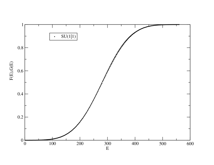
Figure 2: Continuous curve represents the error function G(E) and crosses represent the cumulative distribution function F(E) (at its discontinuity points) for $SU(1|1)$ spin chain with $N=15$.

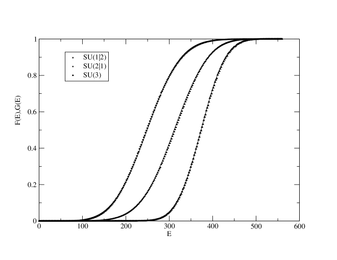
Figure 3: Left continuous curve represents G(E) for $SU(1|2)$ spin chain with $N=15$ and the corresponding F(E) is given by crosses. Middle continuous curve represents G(E) for $SU(2|1)$ spin chain with $N=15$ and the corresponding F(E) is given by dots. Right continuous curve represents G(E) for $SU(3)$ spin chain with $N=15$ and the corresponding F(E) is given by triangles.

Now we can compare the cumulative level density $F(E)$ (5.1) with the error function $G(E)$ (5.2), where the values of $\mu$ and $\sigma$ are obtained from eqns.(5.8) and (5.11) respectively for any given $m$, $n$ and $N$. In Fig.2, we plot such $F(E)$ and $G(E)$ for the particular case of $SU(1|1)$ spin chain with $N=15$ lattice sites. From this figure it is evident that $F(E)$ follows $G(E)$ to a high degree of approximation. One can also quantify the agreement between $F(E)$ and $G(E)$ by calculating the corresponding mean square error (MSE), which for the above mentioned case is given by $8.46\times 10^{-6}$. It may be noted that, the agreement between $F(E)$ and $G(E)$ improves rapidly with increasing values of $N$. For example, in the case of $SU(1|1)$ model, MSE between $F(E)$ and $G(E)$ decreases from $5.17\times 10^{-5}$ to $8.46\times 10^{-6}$ when the value of $N$ is increased from $10$ to $15$. Next, we consider the particular cases of $SU(1|2)$ as well as $SU(2|1)$ supersymmetric spin chain with $N=15$ lattice sites and also the $SU(3)$ bosonic spin chain with same number of lattice sites for the sake of comparison. In Fig.3, we plot $F(E)$ and $G(E)$ for $SU(1|2)$, $SU(2|1)$ and $SU(3)$ HS spin chains and find that the corresponding MSEs are given by $2.38\times 10^{-5}$, $1.2\times 10^{-5}$ and $8.61\times 10^{-6}$ respectively. Again $F(E)$ shows very good agreement with $G(E)$ for all of these cases. Such agreement also improves rapidly with increasing values of $N$. For example, in the case of $SU(1|2)$ spin chain, MSE between $F(E)$ and $G(E)$ decreases from $8.23\times 10^{-5}$ to $2.38\times 10^{-5}$ when the value of $N$ is increased from $10$ to $15$. Analysing many other particular cases with different values of $m,~{}n$ and sufficiently large values of $N$, we find that $F(E)$ follows $G(E)$ with a high degree of approximation for all of these cases.

From the above discussion it is evident that the local fluctuations in energy level distribution, as shown in Fig.1 for the particular case of $SU(1|1)$ spin chain, get cancelled very rapidly whenever we take the cumulative sum of such distribution. Furthermore, for sufficiently large values of $N$, continuous part of the level density distribution in the spectrum of supersymmetric HS spin chain satisfies the Gaussian approximation at the same high level of accuracy as in the pure bosonic case. It may be noted that, the level density of embedded Gaussian orthogonal ensemble (GOE) also follows Gaussian distribution at the limit $N\rightarrow\infty$, provided the number of one-particle states tends to infinity faster than $N$ [21]. However, in our case of $SU(m|n)$ HS spin chain, the number of one-particle states (i.e., $m+n$ ) remains fixed for all values of $N$.

Next we want to study the NNS distribution in the spectrum of $SU(m|n)$ HS spin chain. To eliminate the effect of level density variation in the calculation of NNS distribution for the full energy range, it is necessary to apply an unfolding mapping to the ‘raw’ spectrum [22]. This unfolding mapping may be defined by using the continuous part of the cumulative level density distribution. We have already seen that, for the case of $SU(m|n)$ HS spin chain, the continuous part of cumulative level density is given by $G(E)$ (5.2) with a high degree of approximation. So we transform each energy $E_{i}$, $i=1,\cdots,l\,$, into an unfolded energy $\xi_{i}\equiv G(E_{i})$. The function $p(u)$ is defined as the density of the normalized spacings $u_{i}=(\xi_{i+1}-\xi_{i})/\Delta$, where $\Delta=(\xi_{l}-\xi_{1})/(l-1)$ is the mean spacing of the unfolded energy. To get rid of local fluctuations occurring in $p(u)$, again we study the cumulative NNS distribution given by $P(u)=\int_{0}^{u}p(x)dx$, instead of $p(u)$. In this context it may be noted that, NNS distributions corresponding to the cases of classical GOE as well as embedded GOE obey the Wigner’s law [23]:

$$p(u)=\frac{\pi}{2}u\exp(-\pi u^{2}/4)\,.$$

On the other hand, from the conjecture of Berry and Tabor one may expect that the NNS distribution for an integrable model will obey Poisson’s law given by $p(u)=\exp(-u)$ [24]. However, it has been found that the NNS distribution for $SU(m)$ bosonic HS spin chain does not follow either Wigner’s law or Poisson’s law within a wide range of $N$ [9]. Instead, the cumulative NNS distribution for this bosonic spin chain can be well approximated by a function like

$$\tilde{P}(u)=v^{\alpha}[1-\gamma(1-v)^{\beta}],$$ (5.12)

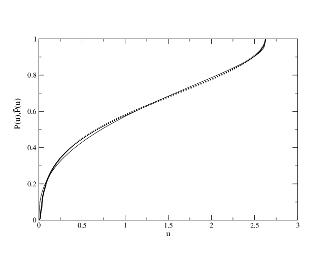
Figure 4: Dotted curve represents the cumulative NNS distribution $P(u)$ for $SU(1|1)$ spin chain with $N=17$ and the continuous curve represents the approximate distribution function $\tilde{P}(u)$.

where $v=u/u_{max}$ with $u_{max}$ being the largest normalized spacing, $\alpha$ and $\beta$ are two free parameters taking values within the range $0<\alpha,~{}\beta<1$, and the value of $\gamma$ is fixed by requiring that the average normalized spacing be equal to 1. In our study we also find that, NNS distribution in the spectrum of $SU(m|n)$ HS spin chain does not follow either Wigner’s law or Poisson’s law within a wide range of $N$. In particular, it is observed that the slope of cumulative NNS distribution diverges for both $u\rightarrow 0$ and $u\rightarrow u_{max}$, which can not be explained from Wigner’s or Poisson’s distribution. Furthermore, we find that the cumulative NNS distribution for $SU(m|n)$ HS spin chain can be fitted well by $\tilde{P}(u)$ in eqn.(5.12) within a range of $N$. For example, in the particular case of $SU(1|1)$ spin chain, it is checked that $P(u)$ agrees well with $\tilde{P}(u)$ within the range $N\leq 20$. In Fig.4, we plot such $P(u)$ and $\tilde{P}(u)$ for $N=17$ lattice sites ($u_{max}=2.626$ in this case) and found a good agreement with MSE $=0.0234$ when the values of free parameters are taken as $\alpha=0.39$ and $\beta=0.29$. However, it is possible that the appearance of such non-Poissonian NNS distribution in the spectrum of $SU(m|n)$ HS spin chain is an artifact of finite-size effect, which requires further investigation.

Finally we want to make a comment about the behaviour of parameters $\mu$ in eqn.(5.8) and $\sigma$ in eqn.(5.11) under the exchange of bosonic and fermionic spin degrees of freedom. Since $s\rightarrow s$ and $t\rightarrow-t$ under this exchange, we find that $\sigma$ remains invariant and $\mu$ changes to $\bar{\mu}$ given by $\bar{\mu}=\frac{N(N^{2}-1)}{6}-{\mu}\,$. It is interesting to note that this relation between $\mu$ and $\bar{\mu}$ can also be obtained by applying eqn.(4.12):

$${\mu} = \frac{1}{s^{N}}\sum_{E_{i}}\mathcal{D}^{(m|n)}(E_{i})E_{i}$$

$$= \frac{1}{s^{N}}\sum_{E_{i}}\mathcal{D}^{(n|m)}\left(\frac{N(N^{2}-1)}{6}-E_{i}\right)E_{i}=\frac{N(N^{2}-1)}{6}-\bar{\mu}\,.$$

This agreement clearly gives a support to our conjecture (4.11). By using this conjecture we have found in Sec.4 that, the spectrum of $SU(n|m)$ spin chain can be obtained from that of $SU(m|n)$ spin chain through an inversion and overall shift of all energy levels. Since none of these operations change the standard deviation of level density distribution, $\sigma$ should take the same value for $SU(m|n)$ and $SU(n|m)$ HS spin chain. Hence, the observation that $\sigma$ in eqn.(5.11) remains invariant under the exchange of bosonic and fermionic spin degrees of freedom, is also consistent with our conjecture (4.11).

6 Conclusion

Here we derive an exact expression for the partition function of $SU(m|n)$ supersymmetric HS spin chain by using the freezing trick and also study some properties of the related spectrum. For applying the freezing trick, we consider a spin CS model containing an anyon like representation of the permutation algebra as spin dependent interaction. We find out the complete spectrum of such spin CS model including the degeneracy factors of all energy eigenvalues. At the strong coupling limit, this spin CS model reduces to the sum of spinless CS model with only dynamical degrees of freedom and $SU(m|n)$ supersymmetric HS spin chain. Consequently, by factoring out the contribution due to dynamical degrees of freedom from partition function of this spin CS model, we obtain the partition function of $SU(m|n)$ supersymmetric HS spin chain. By using this partition function, we study the motif representation for $SU(m|n)$ HS spin chain and find that, due to the lifting of a selection rule, some additional energy levels appear in the spectrum in comparison with the case of $SU(m)$ bosonic spin chain.

By using Mathematica we observe that, the partition function of $SU(m|n)$ HS model satisfies the duality relation (4.11) for many values of $m,$ $n$ and $N$. This observation motivates us to conjecture that this duality relation, involving the interchange of bosonic and fermionic spin degrees of freedom, is valid for all possible values of $m,$ $n$ and $N$. It would be interesting if this duality relation can be proved analytically by using the motif representations and skew-Young diagrammes associated with the $Y(gl_{(m|n)})$ quantum group. Furthermore, it is known that, the partition functions of $SU(m)$ and $SU(m|n)$ Polychronakos spin chains are intimately connected with Rogers-Szegö (RS) polynomial [8,15], which appears in the theory of partitions [25]. Since, HS spin chain share the same quantum group symmetry with Polychronakos spin chain, it might be promising to investigate mathematical structures connected with the partition functions of $SU(m)$ as well as $SU(m|n)$ HS spin chain and explore whether some new RS type polynomials can be generated in this way.

By using the partition function of $SU(m|n)$ HS spin chain, we study global properties of its spectrum like level density distribution and NNS distribution. It is found that, similar to the case of $SU(m)$ bosonic HS spin chain, continuous part of the energy level density satisfies the Gaussian distribution with a high degree of accuracy for sufficiently large values of $N$. We also derive exact expressions for the mean value and the standard deviation which characterize such Gaussian distribution. It would be interesting to provide an explanation for this behaviour of energy level density distribution in the framework of random matrix theory and explore whether the underlying quantum group symmetry of HS spin chain plays some role in this matter.

Acknowledgements

We would like to thank Palash B. Pal for some helpful discussions.

Appendix A. Evaluation of trace formulas

Here we shall derive the trace formulas (5.4a,b,c,d) by assuming that $|\alpha_{1}\dots\alpha_{N}\rangle$ (with $\alpha_{j}\in[1,\dots,s]$) are orthonormal set of vectors. Since the trace of identity operator is given by the dimension of the Hilbert space, eqn.(5.4a) is really a trivial relation. Using eqn.(2.6), it can be shown that

$$\langle\alpha_{1}\dots\alpha_{i}\dots\alpha_{j}\dots\alpha_{N}|\tilde{P}_{ij}^{(m|n)}|\alpha_{1}\dots\alpha_{i}\dots\alpha_{j}\dots\alpha_{N}\rangle=(-1)^{\epsilon(\alpha_{i})}\delta_{\alpha_{i}\alpha_{j}},$$

where $\epsilon(\alpha_{i})=0~{}(1)$ when $\alpha_{i}$ is a bosonic (fermionic) spin. With the help of above equation, we derive the trace relation (5.4b) as

$$tr\left[\tilde{P}_{ij}^{(m|n)}\right]\hskip-5.69046pt = \hskip-5.69046pt\sum_{\alpha_{1}\dots\alpha_{N}=1}^{s}\langle\alpha_{1}\dots\alpha_{i}\dots\alpha_{j}\dots\alpha_{N}|\tilde{P}_{ij}^{(m|n)}|\alpha_{1}\dots\alpha_{i}\dots\alpha_{j}\dots\alpha_{N}\rangle$$

$$= ~{}\sideset{}{{}^{(\alpha_{i},\alpha_{j})}}{\sum}_{\alpha_{1}\dots\alpha_{N}=1}^{s}\sum_{\alpha_{i},\alpha_{j}=1}^{s}\,\langle\alpha_{1}\dots\alpha_{i}\dots\alpha_{j}\dots\alpha_{N}|\tilde{P}_{ij}^{(m|n)}|\alpha_{1}\dots\alpha_{i}\dots\alpha_{j}\dots\alpha_{N}\rangle$$

$$= ~{}\sideset{}{{}^{(\alpha_{i},\alpha_{j})}}{\sum}_{\alpha_{1}\dots\alpha_{N}=1}^{s}\sum_{\alpha_{i}=1}^{s}(-1)^{\epsilon(\alpha_{i})}=s^{N-2}t,$$

where the notation $\sideset{}{{}^{(\alpha_{i},\alpha_{j})}}{\sum}\limits_{\alpha_{1}\dots\alpha_{N}=1}^{s}$ represents summation over all spin components $\alpha_{1},\dots,\alpha_{N}$ except $\alpha_{i}$ and $\alpha_{j}$.

Next, by using eqn.(2.6), it is found that

$$~{}~{}~{}~{}~{}~{}~{}~{}~{}~{}\langle\alpha_{1}\dots\alpha_{i}\dots\alpha_{j}\dots\alpha_{l}\dots\alpha_{N}|\tilde{P}_{ij}^{(m|n)}\tilde{P}_{il}^{(m|n)}|\alpha_{1}\dots\alpha_{i}\dots\alpha_{j}\dots\alpha_{l}\dots\alpha_{N}\rangle=\delta_{\alpha_{i}\alpha_{j}}\delta_{\alpha_{i}\alpha_{l}}.$$

Applying the above equation, we obtain a trace relation in eqn.(5.4c) as

$$\begin{split}&tr\left[\tilde{P}_{ij}^{(m|n)}\tilde{P}_{il}^{(m|n)}\right]\\ &~{}~{}~{}~{}=\sum_{\alpha_{1}\dots\alpha_{N}=1}^{s}\langle\alpha_{1}\dots\alpha_{i}\dots\alpha_{j}\dots\alpha_{l}\dots\alpha_{N}|\tilde{P}_{ij}^{(m|n)}\tilde{P}_{il}^{(m|n)}|\alpha_{1}\dots\alpha_{i}\dots\alpha_{j}\dots\alpha_{l}\dots\alpha_{N}\rangle\\ &~{}~{}~{}~{}=~{}~{}\sideset{}{{}^{(\alpha_{i},\alpha_{j},\alpha_{l})}}{\sum}_{\alpha_{1}\dots\alpha_{N}=1}^{s}\sum_{\alpha_{i}=1}^{s}1=s^{N-2}.\end{split}$$

Other trace relations in (5.4c) can be proved in a similar way.

By using eqn.(2.6), it is also found that

$$\langle\alpha_{1}\dots\alpha_{i}\dots\alpha_{j}\dots\alpha_{k}\dots\alpha_{l}\dots\alpha_{N}|\,\tilde{P}_{ij}^{(m|n)}\tilde{P}_{kl}^{(m|n)}\,|\alpha_{1}\dots\alpha_{i}\dots\alpha_{j}\dots\alpha_{k}\dots\alpha_{l}\dots\alpha_{N}\rangle~{}~{}~{}~{}~{}~{}~{}~{}~{}~{}~{}~{}~{}~{}~{}$$

$$~{}~{}~{}~{}~{}~{}~{}~{}~{}~{}~{}~{}~{}~{}~{}~{}~{}~{}~{}~{}~{}~{}~{}~{}=(-1)^{\epsilon(\alpha_{i})+\epsilon(\alpha_{k})}\,\delta_{\alpha_{i}\alpha_{j}}\delta_{\alpha_{k}\alpha_{l}}\,.$$

With the help of this equation, we obtain the trace relation (5.4d) as

$$\begin{split}&tr\left[\tilde{P}_{ij}^{(m|n)}\tilde{P}_{kl}^{(m|n)}\right]\\ &=\sum_{\alpha_{1}\dots\alpha_{N}=1}^{s}\langle\alpha_{1}\dots\alpha_{i}\dots\alpha_{j}\dots\alpha_{k}\dots\alpha_{l}\dots\alpha_{N}|\tilde{P}_{ij}^{(m|n)}\tilde{P}_{kl}^{(m|n)}|\alpha_{1}\dots\alpha_{i}\dots\alpha_{j}\dots\alpha_{k}\dots\alpha_{l}\dots\alpha_{N}\rangle\\ &=~{}~{}\sideset{}{{}^{(\alpha_{i},\alpha_{j},\alpha_{k},\alpha_{l})}}{\sum}_{\alpha_{1}\dots\alpha_{N}=1}^{s}\sum_{\alpha_{i},\alpha_{k}=1}^{s}(-1)^{\epsilon(\alpha_{i})+\epsilon(\alpha_{k})}=s^{N-4}t^{2}.\end{split}$$

Appendix B. Evaluation of summation formulas

Here we briefly describe the way of calculating known summation formulas (5.7a) and (5.7b) [9], and subsequently present our derivation for new ones like (5.7c) and (5.7d). From the work of Calogero et. al [20], it is known that

$$\sum_{j=1}^{N-1}\frac{1}{\sin^{2}(\frac{j\pi}{N})}=\frac{N^{2}-1}{3}\,,$$ (B-1)

and

$$\sum_{j=1}^{N-1}\frac{1}{\sin^{4}(\frac{j\pi}{N})}=\frac{(N^{2}-1)(N^{2}+11)}{45}\,.$$ (B-2)

Using the translational invariance on a circular lattice and summation relation (B-1), one can obtain eqn.(5.7a) as

$$R_{0}=\frac{1}{2}\sum_{i\neq j}\frac{1}{\sin^{2}(\xi_{i}-\xi_{j})}=\frac{N}{2}\sum_{j=1}^{N-1}\frac{1}{\sin^{2}\left(\frac{j\pi}{N}\right)}=\frac{N(N^{2}-1)}{6}\,.$$

Similarly, by using (B-2), one obtains eqn.(5.7b) as

$$R_{1}=\frac{1}{2}\sum_{i\neq j}\frac{1}{\sin^{4}(\xi_{i}-\xi_{j})}=\frac{N}{2}\sum_{j=1}^{N-1}\frac{1}{\sin^{4}\left(\frac{j\pi}{N}\right)}=\frac{N(N^{2}-1)(N^{2}+11)}{90}.$$

For the purpose of calculating $R_{2}$ in eqn.(5.5c), we note that $R_{0}$ in eqn.(5.5a) can be expressed as

$$R_{0}=\sum_{\begin{subarray}{c}k<l\\ (k,l\neq i,j)\end{subarray}}\frac{1}{\sin^{2}(\xi_{k}-\xi_{l})}+\sum_{\begin{subarray}{c}r=1\\ (r\neq i)\end{subarray}}^{N}\frac{1}{\sin^{2}(\xi_{i}-\xi_{r})}+\sum_{\begin{subarray}{c}r=1\\ (r\neq j)\end{subarray}}^{N}\frac{1}{\sin^{2}(\xi_{j}-\xi_{r})}-\frac{1}{\sin^{2}(\xi_{i}-\xi_{j})}.$$

Substituting the value of $R_{0}$ given in (5.7a) to the above relation and also using (B-1), we find that

$$\sum_{\begin{subarray}{c}k<l\\ (k,l\neq i,j)\end{subarray}}\frac{1}{\sin^{2}(\xi_{k}-\xi_{l})}=\frac{(N^{2}-1)(N-4)}{6}+\frac{1}{\sin^{2}(\xi_{i}-\xi_{j})}\,.$$

By substituting this expression to $R_{2}$ in eqn.(5.5c), and subsequently using eqns.(5.7a) as well as (5.7b), we derive the value of $R_{2}$ given in eqn.(5.7c) as

$$R_{2} = \sum_{i<j}\frac{1}{\sin^{2}(\xi_{i}-\xi_{j})}\biggl{[}\frac{(N^{2}-1)(N-4)}{6}+\frac{1}{\sin^{2}(\xi_{i}-\xi_{j})}\biggr{]}$$

$$= \frac{N(N^{2}-1)^{2}(N-4)}{36}+\frac{N(N^{2}-1)(N^{2}+11)}{90}\,.$$

Finally, by substituting the values of $R_{0}$ (5.7a), $R_{1}$ (5.7b) and $R_{2}$ (5.7c) to the relation (5.6), we easily obtain the value of $R_{3}$ appearing in eqn.(5.7d).

References

1. F. D. M. Haldane, Phys. Rev. Lett. 60 (1988) 635.

2. B. S. Shastry, Phys. Rev. Lett. 60 (1988) 639.

3. F. D. M Haldane, in Proc. 16th Taniguchi Symp., Kashikojima, Japan (1993), eds. A. Okiji and N. Kawakami (Springer, 1994).

4. Z.N.C. Ha, Quantum many-body systems in one dimension (Series on Advances in Statistical Mechanics, Vol.12), (World Scientific,1996).

5. A.P. Polychronakos, Generalized statistics in one dimension, Les Houches 1998 lectures, hep-th/9902157.

6. F. D. M. Haldane, Z.N.C. Ha, J.C. Talstra, D. Benard and V. Pasquier, Phys. Rev. Lett. 69 (1992) 2021.

7. D. Benard, M. Gaudin, F. D. M. Haldane, and V. Pasquier, J. Phys. A26 (1993) 5219.

8. K.Hikami, Nucl. Phys. B441[FS] (1995) 530.

9. F. Finkel, A. González-López, Phys. Rev. B72 (2005) 174411.

10. A.P. Polychronakos, Phys. Rev. Lett. 70 (1993) 2329; Nucl. Phys. B419 (1994) 553.

11. Bill Sutherland and B. S. Shastry, Phys. Rev. Lett. 71 (1993) 5.

12. A.P. Polychronakos, Physics and mathematics of Calogero particles, hep-th/0607033.

13. P. Schlottmann, Int. Jour. Mod. Phys. B11 (1997) 355.

14. B. Basu-Mallick, H. Ujino and M. Wadati, Jour. Phys. Soc. Jpn. 68 (1999) 3219.

15. K. Hikami, and B. Basu-Mallick, Nucl. Phys. B566 [PM] (2000) 511.

16. B. Basu-Mallick, Nucl. Phys. B540 [FS] (1999) 679.

17. B. Basu-Mallick, Nucl. Phys. B482 [FS] (1996) 713.

18. C. Ahn and W. M. Koo, Phys. Lett. B365 (1996) 105.

19. B. Sutherland, Phys. Rev. A5 (1972) 1372.

20. F. Calogero and A.M. Perelomov, Commun. Math. Phys. 59 (1978) 109.

21. K.K. Mon and J.B. French, Ann. Phys. 95 (1975) 90.

22. F. Haake, Quantum signatures of Chaos (Springer-verlag, 2001).

23. V.K.B. Kota, Phys. Rep. 347 (2001) 223.

24. M.V. Berry and M. Tabor, Proc. R. Soc. Lond. A356 (1977) 375.

25. G.E. Andrews, The theory of partitions (Addison-Wesley, Reading, M.A., 1976).

Figure 1: Energy levels $E_{i}$ and degeneracies $\mathcal{D}^{(1|1)}(E_{i})$ of the $SU(1|1)$ HS spin chain for $N=15$.