Cosmic Perturbations Through the Cyclic Ages

Abstract

We analyze the evolution of cosmological perturbations in the cyclic model, paying particular attention to their behavior and interplay over multiple cycles. Our key results are: (1) galaxies and large scale structure present in one cycle are generated by the quantum fluctuations in the preceding cycle without interference from perturbations or structure generated in earlier cycles and without interfering with structure generated in later cycles; (2) the ekpyrotic phase, an epoch of gentle contraction with equation of state $w\gg 1$ preceding the hot big bang, makes the universe homogeneous, isotropic and flat within any given observer’s horizon; and, (3) although the universe is uniform within each observer’s horizon, the global structure of the cyclic universe is more complex, owing to the effects of superhorizon length perturbations, and cannot be described in a uniform Friedmann-Robertson-Walker picture. In particular, we show that the ekpyrotic phase is so effective in smoothing, flattening and isotropizing the universe within the horizon that this phase alone suffices to solve the horizon and flatness problems even without an extended period of dark energy domination (a kind of low energy inflation). Instead, the cyclic model rests on a genuinely novel, non-inflationary mechanism (ekpyrotic contraction) for resolving the classic cosmological conundrums.

I Introduction

Cosmological observations support the idea that the part of the universe we now observe emerged from a hot, radiation dominated and expanding state. The original hot big bang theory did not specify how this radiation was generated. Inflationary theory Guth (1981) postulates a phase of superluminal expansion, driven by scalar field potential energy which ultimately decays into radiation. By contrast, in the ekpyrotic Khoury et al. (2001) model, the radiation is generated by a brane collision, following an earlier empty phase. The earlier phase is contracting from the viewpoint of Einstein-frame four dimensional effective theory. A transition from Einstein-frame contraction to expansion is also invoked in the pre-big bang model Gasperini and Veneziano (1993).

Both the inflationary Bardeen et al. (1983); Guth and Pi (1982); Hawking (1982) and ekpyrotic models Khoury et al. (2001, 2002); Tolley et al. (2004) plausibly give a spectrum of primordial fluctuations that is nearly scale invariant and adiabatic, in accordance with recent cosmic microwave background Spergel et al. (2003) and large scale structure Tegmark et al. (2004) observations. Indeed, these two theories seem to be the only ones that are generically able to give such predictions Gratton et al. (2004).

However, both theories are incomplete. For inflation, it seems inevitable that an initial singularity is still present Borde et al. (2003) (but see Aguirre and Gratton (2002, 2003)) only a finite affine parameter distance away, meaning that initial conditions at the singularity are potentially significant. In the ekpyrotic scenario, the initial emptiness of the contracting phase is not explained.

The cyclic model Steinhardt and Turok (2002a, b) builds on the ekpyrotic one, essentially stacking a whole series of ekpyrotic histories together. One post-bounce expanding phase links onto another contracting phase. This contracting phase passes via a bounce into a new expanding phase, and so on. The universe evolves cyclically, so that the puzzle of a “fundamental beginning of time” is at least deferred into the very distant past, and perhaps avoided altogether.

The ekpyrotic and cyclic models both have a higher dimensional interpretation, inspired by M-theory. This perspective is critical for understanding how perturbations can propagate through a bounce, and much recent work has focussed on this issue Tolley et al. (2004); Craps and Ovrut (2004); Turok et al. (2004). (For varying four dimensional perspectives on the matching see Khoury et al. (2002); Durrer (2001); Durrer and Vernizzi (2002); Cartier et al. (2003); Brandenberger and Finelli (2001); Finelli and Brandenberger (2002); Lyth (2002); Hwang (2002); Peter and Pinto-Neto (2002); Creminelli et al. (2004).) Here we address other critical issues for perturbations in the cyclic model, and are able to use a four dimensional effective description almost throughout. We simply assume the essential features of the five dimensional matching prescription are correct, and apply them to the four dimensional effective theory.

Our analysis shows that the galaxies and large scale structure in any given cycle can be generated by the quantum fluctuations in the preceding cycle without interference from perturbations or structure generated in earlier cycles and without interfering with structure generated in later cycles. The global structure of the cyclic universe is more complex: although the universe can be described as a nearly homogeneous and isotropic within any observer’s horizon, the global structure cannot be characterized by a uniform Friedmann-Robertson-Walker picture. Our results further show that the ekpyrotic phase alone is sufficient for resolving the horizon and flatness problems and that an extended phase of dark energy domination or any other form of inflation is completely unnecessary. This makes it clear that the cyclic model is a genuinely novel, non-inflationary approach to cosmology.

II Overview of the Cyclic Model and its Perturbations

The cyclic model assumes that we live on a brane in a special configuration of a higher dimensional theory such as M-theory. Away from a bounce, the universe can be treated using a four dimensional effective theory consisting of gravity coupled to one or more scalar fields. Assuming the background universe is spatially flat, the metric is

$$ds^{2}=-dt^{2}+a^{2}(t)\,\delta_{ij}dx^{i}dx^{j}$$ (1)

where $a(t)$ is the scale factor. The main imprint of the higher dimensional theory on the effective picture is through the addition of one or more scalar fields $\phi$ with a potential $V(\phi)$. This potential performs many functions in the cyclic model, including that of describing the dark energy responsible for the cosmic acceleration observed today. Through most of this paper, we shall describe the model in terms of a single scalar field, although we note that generically more than one scalar field is involved. The scalar field $\phi$ satisfies

$$\ddot{\phi}+3H\dot{\phi}=-V_{,\phi},$$ (2)

in the background (1), where dots denote derivatives with respect to $t$ and $H\equiv\dot{a}/a$. Ignoring, for simplicity, the coupling between ordinary matter and $\phi$, the Friedmann equation is

$$H^{2}=\frac{1}{3}\left(\rho+\frac{1}{2}\dot{\phi}^{2}+V(\phi)\right)$$ (3)

in reduced Planck units ($8\pi G=1$), where $\rho$ is the energy density of ordinary matter and radiation.

The potential $V(\phi)$ is chosen by hand at present, but should ultimately be derivable from the higher dimensional theory. It must be of a certain form in order for the cyclic model to work Khoury et al. (2004). A useful potential with the desired properties is

$$V(\phi)=V_{0}\left(e^{b\phi}-e^{-c\phi}\right)F\left(\phi\right)$$ (4)

(see Fig. 1). Here $V_{0}$ is of order today’s dark energy density, $b$ is non-negative (and typically $\ll 1$) and $c$ is positive (and typically $\gg 1$). $F(\phi)$ is a function whose precise form is unimportant, but which tends to unity for $\phi$ greater than $\phi_{\text{end}}$ and to zero for $\phi$ less than $\phi_{\text{end}}$. The resulting potential $V(\phi)$ has a large negative minimum, denoted $V_{\text{end}}$, at $\phi_{\text{end}}$. While the explicit exponential form used here is convenient for analysis, note that the cyclic model actually works for a very wide range of potential forms, the only conditions being that they have a steep, negative and strongly negatively curved region over the observationally relevant range of the scalar field.

Figure 1: An example potential $V(\phi)$. This plot shows where $\phi$ is on its potential at each stage in a cycle. The equation of state parameter of the background solution is denoted by $w$.

Of central importance to the cyclic model is the ekpyrotic phase, in which the universe is slowly contracting and the scalar field is rolling slowly down its steeply declining, negative potential. For our example potential, the negative exponential dominates, $V(\phi)\approx-V_{0}e^{-c\phi}$, and the background universe enters an attractor scaling solution,

$$a(t)\propto(-t)^{2/c^{2}}\propto e^{\phi/c},\qquad H={2\over c^{2}t}\propto-e^{-{c\phi/2}},\qquad w\approx c^{2}/3\gg 1,$$ (5)

in which $t$ is negative and increasing, and $w$ is the ratio of the pressure to the energy density. Notice that, since $c\gg 1$, as the scalar field moves over a substantial range in Planck units towards $\phi_{\text{end}}$, the scale factor contracts by only a modest factor. In contrast, the Hubble parameter $H$ grows dramatically, beginning from values comparable to today’s value, and growing to values corresponding to high energy scales.

The scaling solution is only relevant as long as $\phi>\phi_{\text{end}}$, and the function $F(\phi)$ is effectively unity. Once $\phi$ passes the potential minimum, the potential energy is quickly converted to kinetic energy and the solution enters a kinetic energy dominated phase, with

$$a(t)\propto(-t)^{1\over 3}\propto e^{\phi/\sqrt{6}},\qquad H={1\over 3t}\propto-e^{-{\sqrt{2/3}}\phi},\qquad w\approx 1.$$ (6)

When lifted to higher dimensions, this solution describes two colliding branes (one with positive tension and the other with negative tension), whose scale factors remain finite even as the four dimensional scale factor $a(t)$ tends to zero and the scalar field $\phi$ tends to $-\infty$. Near the collision, the four-dimensional Einstein-frame metric and scalar field become singular coordinates; however, five-dimensional quantities like the metric on each brane, and the inter-brane distance, are perfectly finite. The matching of perturbations across the bounce is therefore performed within the higher dimensional setting.

As the branes emerge from the collision, the solution followed is nearly the exact time-reverse of (6); the radiation and matter produced at the bang and a modest enhancement of the kinetic energy of $\phi$ have a negligible effect while $\phi<\phi_{\text{end}}$. There is a brief $w\gg 1$ expanding phase after $\phi$ passes $\phi_{\text{end}}$ moving to positive values, but the excess kinetic energy in $\phi$ quickly overwhelms the potential energy $V(\phi)$ and the universe enters a second expanding kinetic phase (Figure 1). As is shown in the Appendix, the expanding $w\gg 1$ phase is of modest duration and for the remainder of this paper it can be safely ignored. It is then convenient to describe all three kinetic energy dominated phases, namely the contracting and expanding kinetic phases with $\phi<\phi_{\text{end}}$, and the second expanding kinetic phase with $\phi>\phi_{\text{end}}$, as a single kinetic phase, and we shall generally adopt this terminology throughout the remainder of this paper.

As we continue into the expanding phase, the kinetic energy in $\phi$ redshifts away as $a^{-6}$ and the universe becomes dominated by the radiation that was produced at the bounce. The net expansion in the entire kinetic phase is $\sim e^{2\gamma/3}$, where $\gamma\equiv\ln((-V_{\text{end}})^{1/4}/T_{\text{rh}})$, and $T_{\text{rh}}$ is by definition the temperature of the radiation when it comes to dominate. As shown in Ref. Khoury et al. (2004), cyclic models require $\gamma\sim 10-20$ in order to be compatible with observation. The additional Hubble damping due to the radiation has the effect of slowing $\phi$ down to a halt on the positive potential plateau. Then, the scalar field begins to gently roll downhill. The matter era passes and the universe enters the dark energy phase. Eventually, the rolling of $\phi$ carries it off the plateau. The accelerated expansion due to dark energy reverses to slow ekpyrotic contraction. The universe heads towards the next bounce and the next cosmic cycle.

The evolution of the background universe is illustrated by the inner, solid, track of the “wheel” of Fig. 2. Fig. 1 has also been labelled to show where $\phi$ is on its potential at each stage in the cycle. See also Fig. 4 for a summary of the behavior of key quantities.

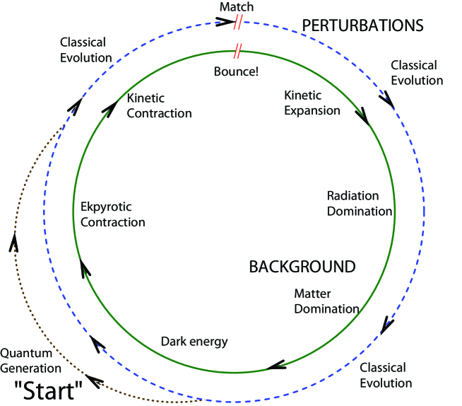
Figure 2: A “wheel” diagram indicating the behavior of both the background solution (inner, solid, line) and perturbations (outer, dashed and dotted, lines) in the cyclic model. “Start” marks the point in the cycle at which our perturbation analysis in Sec. III begins.

Note that while the bounce itself is nearly symmetrical, the background evolution for $\phi>\phi_{\text{end}}$ is highly asymmetrical, and the scale factor undergoes a large net expansion from cycle to cycle. As explained above, the kinetic phase gives a net expansion of ${2\over 3}\gamma$ e-folds. The ensuing radiation phase gives a large number of e-folds of expansion, and the matter phase adds a few more. We may approximate the combined number from the latter two phases as $N_{\text{rad}}\equiv\ln(T_{\text{rh}}/T_{0})$, where $T_{0}$ is the cosmic microwave background temperature today. Dark energy adds another potentially large number of e-folds $N_{\text{dark}}$. By contrast, in the ekpyrotic contraction phase, the scale factor contracts by a very modest factor (from Eq. 5, $a\propto H^{2/3w}$). So there is a large net expansion every cycle of approximately $2\gamma/3+N_{\text{rad}}+N_{\text{dark}}$ e-folds, which is critical for the fate of the model when perturbations are considered (see Sec. VI). The large net expansion also plays a key role in diluting the entropy density from cycle to cycle, and, as we shall see in Sec. VIII, in the cyclic model’s solution to the flatness, isotropy and horizon puzzles.

While the scale factor grows with each new cycle, locally measurable quantities like the Hubble parameter and the density undergo periodic evolution. The Hubble parameter decreases by $2\gamma$ e-folds in the second kinetic energy dominated expanding phase, and by $2N_{\text{rad}}$ e-folds in the ensuring radiation phase. By contrast, in the ekpyrotic contracting phase, $H$ increases in magnitude very rapidly, by a total of $N_{\text{ekp}}\equiv\ln\left(\sqrt{-V_{\text{end}}/V_{0}}\right)$ e-folds. Since $V_{0}\sim T_{0}^{4}$ in order of magnitude, we find $N_{\text{ekp}}\approx 2(N_{\text{rad}}+\gamma)$, which is also the condition that the Hubble constant returns to its original magnitude after a cycle.

In this paper, for the study of perturbations, we shall consider a universe that contains, in addition to the scalar field $\phi$, cold dark matter and radiation, which we treat as perfect fluids. This description captures the broad features of cosmology well enough for our purposes. The metric has scalar, vector and tensor perturbations. We assume that the perturbations can be well treated in linear theory, in which case the three sectors decouple and we can follow perturbations Fourier mode by Fourier mode. We ignore the vectors and tensors, and concentrate on the scalar sector, in which the matter density perturbations exist. We work in longitudinal gauge, in which there are no time-space or traceless space-space perturbations. Perfect fluids and scalar fields do not support anisotropic stress, so the gravitational potentials are equal, and the perturbed metric reduces to:

$$ds^{2}=-(1+2\Phi)dt^{2}+a^{2}(t)\,(1-2\Phi)\delta_{ij}dx^{i}dx^{j},$$ (7)

where $\Phi$ is the Newtonian potential.

Within any one cycle, the Einstein and matter equations fully determine the classical evolution of the perturbations. This classical evolution is indicated by the outer, dashed loop of our wheel diagram (Fig. 2).

The cyclic model, like inflation, relies on the amplification of quantum fluctuations to initiate structure formation. It is helpful to think in the Heisenberg picture. Here the quantum field mode operators satisfy the classical equations of motion but even if the quantum expectation value of a mode amplitude is zero, the expected variance cannot also be zero (just as for the ground state of a simple harmonic oscillator, for example). When the equation governing a mode moves from having oscillatory solutions to growing and decaying solutions, the quantum variance will also grow, as the square of the classical growing mode amplitude. As far as the evaluation of future expectation values is concerned, it now becomes possible to accurately approximate the quantum picture with a classical one in which the mode amplitude is treated as a random variable with mean and variance given by the quantum calculation. We say that a perturbation has been generated when the classical probabilistic description becomes accurate. In the cyclic model perturbations can be generated during both the dark energy and ekpyrotic phases, and quantum fluctuations in one cycle become classical stochastic perturbations by the next. Of course, this stochastic contribution to a mode amplitude is only important if it is comparable to or greater than that which is already there from the classical evolution. “Quantum generation” of perturbations is represented by the dotted line in the wheel diagram, Fig. 2.

To complete the perturbation loop in our wheel diagram we need to know how to match perturbations across a bounce. This is the one place where the four-dimensional effective picture becomes invalid and results obtained in higher dimensions must be used. Recent work Tolley et al. (2004); Turok et al. (2004); McFadden et al. (2005) suggests how this occurs, with long-wavelength growing modes going in to the crunch matching onto growing modes going out from the bang. This matching occurs in a manner that, for long wavelengths, is independent of wavelength.

Hence we are now able to follow perturbations through multiple cycles in the cyclic model, allowing for both quantum generation and matching across the bounce in addition to the classical evolution.

III Quantum Generation of Perturbations

In principle, when describing a cyclic model, one can start anywhere on the wheel diagram, Fig. 2. For simplicity, we start well into a long-lasting dark energy phase in which the universe has become very homogeneous and flat and any pre-existing matter, radiation, or scalar field perturbations have been redshifted away to negligible levels. Later on, in Sec. VI, we show that the consistency of the model does not require that the dark energy phase be long-lasting.

In a universe containing only a scalar field $\phi$, the Einstein equations fix the scalar field fluctuation $\delta\phi$ in terms of the Newtonian potential $\Phi$ and its time derivative:

$$\frac{\dot{\phi}}{2}\delta\phi=\dot{\Phi}+H\Phi.$$ (8)

Thus there is only one true scalar degree of freedom, which we take to be $\Phi$, and $\Phi$ satisfies the second-order differential equation:

$$\ddot{\Phi}+\biggl{(}H-\frac{2\ddot{\phi}}{\dot{\phi}}\biggr{)}\dot{\Phi}+2\biggl{(}\dot{H}-\frac{H\ddot{\phi}}{\dot{\phi}}\biggr{)}\Phi-\frac{\nabla^{2}\Phi}{a^{2}}=0.$$ (9)

This equation can be used both for the classical evolution of $\Phi$ and, as discussed above, for determining the variance of the fluctuations generated quantum mechanically. Since, by assumption, there are initially no classical perturbations, we turn to the quantum case.

For the quantum calculation we need to pick a suitable quantum state for each Fourier mode. Just as in inflation, we assume that when the evolution of a perturbation mode is “gradient dominated” (sometimes called “subhorizon”), the scalar field fluctuation $\delta\phi$ is in the appropriate incoming adiabatic vacuum state. Eq. (8) is then used to determine the state of $\Phi$ in this period (see e.g. Khoury et al. (2002)). We then evolve forward in time using (9) until the spatial gradients become negligible in the time evolution. Now, the mode is said to evolve in an “ultralocal” (sometimes called “superhorizon”) manner. The modulus squared of the mode amplitude then gives the quantum variance which, when the quantum picture is replaced by the stochastic classical one, becomes the classical power spectrum on that scale. Repeating the calculation for different comoving wavenumbers allows us to build up the complete power spectrum. The power on a given scale changes with time in accordance with Eq. (9), but all modes that are in the long-wavelength, ultralocal regime will evolve in concert.

We perform the above procedure, solving Eq. (9) mode by mode with the appropriate initial conditions, to build up a power spectrum for the perturbations. All modes of interest start off gradient dominated and end up in the ultralocal regime. Longer wavelength modes start to follow ultralocal evolution sooner, shorter wavelength modes later. The very shortest wavelength modes go ultralocal only in the kinetic energy dominated phase just before the big crunch. Once all modes have gone ultralocal, the whole power spectrum evolves in concert and simply grows in amplitude as the bounce is approached.

The detailed shape of the power spectrum depends on the exact background evolution and the specific details of the scalar field potential $V(\phi)$. Fig. 3 shows a power spectrum for a typical model (with $b=0.1$ and $c=30$), evaluated close to the crunch when all the modes are evolving ultralocally. The comoving wavenumber is denoted by $k$. Observe that there are large bands of $k$ for which the power spectrum is almost scale invariant. Note that there is a feature in the power spectrum on scales $k_{\text{tran}}$ that went ultralocal at around the time of the transition from expansion to contraction. Also note that modes on larger scales (which went ultralocal in the dark energy phase) have a comparable amplitude to those on smaller scales (which went ultralocal in the ekpyrotic contraction phase).

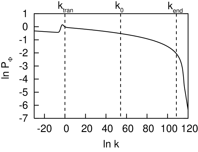
Figure 3: A plot of the power spectrum $P_{\Phi}$ of quantum-generated fluctuations in the Newtonian potential $\Phi$ going into the crunch. A horizontal line corresponds to scale invariance. $k_{\text{end}}$ indicates the wavenumber of the last modes to go ultralocal during ekpyrotic contraction. $k_{0}$ indicates the scale corresponding to our horizon today. The parameters chosen in Eq. (4) are $b=0.1$ and $c=30$.

The range in $\ln k$ of modes to the left of the feature is of order $N_{\text{dark}}$, the number of e-folds of dark energy expansion, while the range of modes to the right of the feature is of order $N_{\text{ekp}}\equiv\ln\sqrt{-V_{\text{end}}/V_{0}}$. As we explain later (Sec. V), the value of $k$ for modes on our current horizon scale is approximately $N_{\text{ekp}}/2$ e-folds to the left of $k_{\text{end}}$ and hence near the middle of the approximately scale-invariant region of the power spectrum.

IV Matching Perturbations through the Bounce

Now we map perturbations through the singularity. First we relate physical length scales on either side of the bounce. Second, we relate the Newtonian potential for each mode on either side of the bounce.

The first task is simplified by the near symmetry of the contracting and expanding kinetic phases. Consider the wavelength of the last mode to go ultralocal during ekpyrotic contraction, with wavenumber $k_{\text{end}}$ in Fig. 3. Its physical wavelength is roughly given by the Hubble radius at that time, $\sim 1/\sqrt{-V_{\text{end}}}$. By the symmetry of the kinetic phases, its physical wavelength when $\phi$ reaches $\phi_{\text{end}}$ on the way out after the bounce will again be $\sim 1/\sqrt{-V_{\text{end}}}$.

For the second task, we need to know how the Newtonian potential behaves on either side of the bounce in the four-dimensional effective treatment. All modes become ultralocal as the bounce is approached, and so all behave in the same manner, independent of their wavelength. If $t=0$ corresponds to the bounce, the Newtonian potential goes like $A+B\,t^{-4/3}$ on the way in and as $A^{\prime}+B^{\prime}\,t^{-4/3}$ on the way out (see Sec. VII). So each side has a diverging term and a constant term. On the way in, the constant term is the “decaying” mode while the $t^{-4/3}$ term is the growing mode. On the way out, the roles are reversed with the constant term now the “growing” mode and the $t^{-4/3}$ term now the decaying mode.

The perturbations are in the growing mode approaching the bounce. It is essential for the success of the cyclic model that such perturbations lead to some growing-mode perturbations after the bounce. For the shape of the spectrum to be preserved it is also essential that such mapping occurs in a manner which is at least approximately independent of wavelength.

To perform the mode matching one must move from the four dimensional effective theory into five dimensions (where the bounce now corresponds to the extra dimension momentarily contracting to zero size and then expanding again). The work of Tolley, Turok and Steinhardt Tolley et al. (2004) does this and provides us with a matrix $\bm{M}_{\text{TTS}}$ that relates the incoming and outgoing mode coefficients. The form of this matrix is presented in Sec. VII, after we have introduced normalized mode functions. According to the matching prescription of Tolley et al. (2004), an incoming growing mode maps onto an outgoing solution with a non-zero growing mode component. Furthermore, the matching is independent of wavelength, as required. The procedure is to find a quantity that behaves as a massless scalar field in a particular five dimensional gauge near the bounce. Earlier work of Tolley and Turok Tolley and Turok (2002) showed that there is a natural way to analytically continue such fields through the bounce. By understanding the correspondence between four and five dimensional perturbations one can thus match four dimensional modes across the bounce. Note that alternative matching prescriptions with alternative matching matrices are straightforward to use in place of $\bm{M}_{\text{TTS}}$. (Indeed, very recent work of McFadden, Turok and Steinhardt McFadden et al. (2005) takes a wider five dimensional view of the vicinity of the collision, and effectively pre- and post-multiplies $\bm{M}_{\text{TTS}}$ by another matrix. However this does not alter the qualitative features of the matching, so $\bm{M}_{\text{TTS}}$ is used in this paper.)

The result of the matching is that after the bounce the “primordial” power spectrum for the expanding phase is in the “growing” mode and has just the same shape as the power spectrum before the bounce (i.e. Fig. 3 again). The amplitude of the power spectrum of the Newtonian potential $\Phi$ is now roughly constant and is determined by three things: the starting amplitude, given by the adiabatic vacuum assumption; the amount of growth occurring during contraction; and finally the precise matching coefficient of growing mode to growing mode in the matching matrix. The parameters controlling the length of the contraction phase (e.g. $\phi_{\text{end}}$) and the details of the bounce (such as the relative speed of the branes at collision) must be chosen to make the perturbation amplitude approximately $10^{-5}$, in order to match observations.

V Classical Evolution of Perturbations

The “primordial” power spectrum computed at the beginning of an expansion cycle can be evolved straightforwardly through to the end of the matter epoch in order to compare it with observation. In this section, we track the perturbations further around the wheel diagram into the dark energy and contraction phases, in order to see what effect they have on the quantum generation of the next round of perturbations. We solve the perturbed Einstein, fluid and scalar field equations numerically mode by mode, starting deep within the radiation era. (All modes of interest follow ultralocal evolution in the kinetic era, so we need not worry about the evolution there.) Our numerical code employs synchronous gauge, but we express the results in terms of the fully gauge-fixed Newtonian gauge potential $\Phi$.

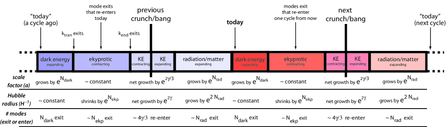
Figure 4: A timeline of the cyclic universe showing the behavior of key quantities over the course of a cycle. The labels “$k_{\text{tran}}$ exits” and “$k_{\text{end}}$ exits” show the times where these two modes start to follow ultralocal evolution (i.e. when spatial gradients become negligible).

The perturbations are initially set in their adiabatic growing mode when they are all ultralocal (i.e. outside the effective horizon). Observations of the cosmic microwave background and large scale structure are sensitive to scales from our cosmological horizon down to roughly ten e-folds in $k$ smaller. To relate this to our simulations, we need to know what portion of the “primordial” spectrum is relevant to observation. To do this, we work out the difference in $k$ between modes on our horizon today and the last modes generated during ekpyrotic contraction. As mentioned in the previous section the physical wavelength of the latter modes is roughly $1/\sqrt{-V_{\text{end}}}$ when $\phi$ passes $\phi_{\text{end}}$ in the expanding phase. Since then there has been a brief $w\gg 1$ phase, a second kinetic energy dominated phase, and the radiation and matter phases (see Fig. 1), providing an expansion of $e^{2\gamma/3+N_{\text{rad}}}$ between them. So these modes have a physical wavelength today of order $e^{2\gamma/3+N_{\text{rad}}}/\sqrt{-V_{\text{end}}}$. Modes on the horizon today (having a physical wavelength of order $1/\sqrt{V_{0}}$) thus have a wavelength $e^{-2\gamma/3-N_{\text{rad}}+N_{\text{ekp}}}$ times this, where $N_{\text{ekp}}$ is as introduced previously in Sec. III. The universe reheats to a moderate temperature after the bang. The reheat temperature $T_{\text{rh}}$ is tuned to produce density perturbations of the observed amplitude and to satisfy other constraints. This imposes a constraint on $\gamma$, as defined in Sec. II via the relation $T_{\text{rh}}=e^{-\gamma}(-V_{\text{end}})^{1/4}$ (which implies $N_{\text{rad}}=-\gamma+N_{\text{ekp}}/2$): namely, one needs $\gamma\sim 10-20$ (or $e^{-\gamma}\sim 10^{-(4-8)}$), depending on the value of $c$. For a more precise discussion of the permitted range for $\gamma$, see Ref. Khoury et al. (2004). Thus, the modes on the horizon today have a wavelength that is $e^{-2\gamma/3-N_{\text{rad}}}\sqrt{-V_{\text{end}}/V_{0}}=e^{\gamma/3+N_{\text{ekp}}/2}$ times that of the last modes to be generated in the ekpyrotic phase; the former are a factor of $\gamma/3+N_{\text{ekp}}/2\gtrsim 5+N_{\text{ekp}}/2$ lower in $\ln k$ than the latter. Since $N_{\text{ekp}}$ is very large, of order $100$, modes on our horizon today lie roughly in the middle of the logarithmic $k$ range of modes to the right of the transition feature seen in Fig. 3. The power spectrum is very smooth in the relevant 10 e-folds in $k$ around this point, with only a slight tilt. In Table 1, we present a table of some of the scales mentioned in this paper and give a timeline of the model in Fig. 4.

Table 1: A table showing various scales discussed in this paper relative to today’s horizon. Note that $\gamma\equiv\ln((-V_{\text{end}})^{1/4}/T_{\text{rh}})$, $N_{\text{ekp}}\equiv\ln\sqrt{-V_{\text{end}}/V_{0}}$, and $N_{\text{rad}}\equiv\ln(T_{\text{rh}}/T_{0})=-\gamma+N_{\text{ekp}}/2$.

Length Scale	Size Relative to Today’s Horizon
Today’s horizon	1
Current wavelength of the modes that:
…were on the horizon one cycle ago	$e^{N_{\text{dark}}+2\gamma/3+N_{\text{rad}}}$
…will be on the horizon one cycle from now	$e^{-N_{\text{dark}}-2\gamma/3-N_{\text{rad}}}$
…were the first ones to go ultralocal during	$e^{2\gamma/3+N_{\text{rad}}}$
the ekpyrotic phase one cycle ago
…were the last ones to go ultralocal during	$e^{-N_{\text{ekp}}+2\gamma/3+N_{\text{rad}}}$
the ekpyrotic phase one cycle ago
…will be the first ones to go ultralocal during	$e^{-N_{\text{dark}}}$
the coming ekpyrotic phase of this cycle
…will be the last ones to go ultralocal during	$e^{-N_{\text{dark}}-N_{\text{ekp}}}$
the coming ekpyrotic phase of this cycle

As an example displaying the qualitative behavior of the Newtonian potential, we have studied the case for a potential of the form given in (4) with $b=0.1$ and $c=5$. The code starts with seven e-folds of radiation domination remaining. This is followed by seven e-folds of matter domination and then only two e-folds worth of dark energy domination before ekpyrotic contraction begins. These parameters are not far from those that might give a fully realistic description of the universe, and serve to illustrate the qualitative features of the mode evolution without requiring us to introduce large exponential factors that complicate the numerics.

Fig. 5 presents the Newtonian potential at four different times. Note that, in this plot, a horizontal line corresponds to scale invariance. Moreover, the tilt of the input power spectrum has been neglected, and thus Fig. 5 depicts the transfer function for an exactly scale-invariant power spectrum of the Newtonian potential.

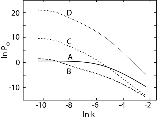
Figure 5: A plot of the power spectrum $P_{\Phi}$ of the Newtonian potential $\Phi$ (in arbitrary units) at various points in a cosmic cycle. $k=1$ corresponds to the horizon at the start of the simulation in the radiation era, and $\ln k\approx-6.6$ corresponds to the horizon at matter-radiation equality. A horizontal line corresponds to scale invariance. The curve A indicates the power at the end of the matter epoch. Curve B indicates the power at turnaround ($H=0$). Curve C indicates the power some way into ekpyrotic contraction, and curve D indicates the power further into the ekpyrotic phase.

In curve A, the power spectrum $P_{\Phi}$ is shown at a time corresponding to “today”, the end of the matter epoch and the beginning of the dark energy epoch. The spectrum is scale invariant at small $k$ and has the expected bend at a scale corresponding to the horizon at matter-radiation equality. At larger wavenumber, the curve falls off as $k^{-4}$. The scalar field fluctuations have had no significant effect on $P_{\Phi}$ at this stage. This curve is in perfect accord with observations.

Curve B shows the power spectrum evolved through the dark energy phase to turnaround at $H=0$. On small scales the power has dropped uniformly as perturbations are diluted.

Curves C and then D show the power spectrum at two stages in the ekpyrotic contraction phase. On large scales the spectrum grows rapidly, and on small scales it reddens. The unstable scalar field contribution dominates the Newtonian potential in this epoch, as matter and radiation are negligible.

VI Interference of perturbations from different cycles

We are now in a position to investigate whether the current perturbations interfere with the quantum generation of the new. First, we compare the amplitude of the current perturbations with that of the new ones to be generated, neglecting any effect that preexisting perturbations might have on the quantum generation of new perturbations. Then we check if this approximation is justified.

We concentrate on scales that are observationally relevant at the beginning of dark energy domination in the next cycle. The mode whose wavelength will equal the current horizon radius one cycle from now is today on a scale that is a factor of roughly $e^{-(N_{\text{dark}}+N_{\text{rad}}+2\gamma/3)}$ times the current horizon radius, the inverse of the total expansion of the universe in the interim, corresponding to $N_{\text{dark}}+N_{\text{rad}}+2\gamma/3$ e-folds in $k$. We saw above that the smallest wavelength mode produced in the ekpyrotic phase lay roughly $N_{\text{rad}}+4\gamma/3$ e-folds within the current horizon. So if there is a significant dark energy phase then there will be negligible power on the scale of the horizon radius in the next cycle. However, as we shall see, an extended period of dark energy domination is not necessary for the cyclic model. To prove the point, we will consider the “worst case scenario,” that the number of e-folds of dark energy domination is negligible. This would put the horizon radius a cycle from now near the high-$k$ downward turn of the “primordial” power spectrum. Since we have only worked to logarithmic accuracy in determining scales, let us conservatively assume that the “primordial” spectrum is still scale invariant even on these small scales. Including the red tilt will only strengthen the argument below showing that there is no obstruction to cycling due to build up of perturbations from cycle to cycle.

We estimate the amplitude of the current perturbations on the relevant scale as follows. The amplitude a mode on our horizon scale has now is roughly $10^{-5}$. In the next section we show that during ekpyrotic contraction the mode grows like $1/t$ with $t$ here the time to the forthcoming bounce. From our numerical results we see that the tilt of the power spectrum on subhorizon scales is reddening as we proceed to the bounce. Asymptotically we expect the mode amplitude to drop as $k^{-4}$ based on the following argument: $\Phi$ from the matter is two powers down from scale-invariant, and this sources a perturbation $\delta\phi$ a further two powers down (see Eq. (15) below, neglecting the time derivative terms). Then when the scalar field is again dominant, Eq. (8) tells us that $\Phi$ should now go like $\delta\phi$, four powers down.

Thus with $k_{0}$ corresponding to our horizon, the amplitude of the current perturbations on a scale $k$ at a time $t$ before the crunch is roughly

$$10^{-5}\,\frac{t_{0}}{t}\left(\frac{k}{k_{0}}\right)^{-4},$$ (10)

where $t_{0}$ is the time from the start of the ekpyrotic phase to the crunch. So the amplitude on our future observer’s horizon is roughly

$$10^{-5}\,\frac{t_{0}}{t}e^{-4N_{\text{rad}}}.$$ (11)

Now let us estimate the amplitude of the new perturbation mode generated on the same scale. The quantum perturbations generated are almost scale invariant, and we exploit this by actually calculating the amplitude of a mode generated in the dark energy phase. The last of these will have been generated just before $t_{0}$, the onset of ekpyrotic contraction. Just as in slow-roll inflation, $\Phi$ will from Eq. (8) then have an amplitude of roughly $\dot{\phi}/H$ times the amplitude of the fluctuation in $\delta\phi$, which is $H$. So $\Phi$ is roughly $\dot{\phi}$ before turnaround, which is of order $H_{0}$, the Hubble constant today. During the contraction the new mode also grows like $1/t$. So at a time $t$ before the crunch, the newly-generated mode amplitude will be of order

$$H_{0}\frac{t_{0}}{t}.$$ (12)

Comparing (11) and (12) we see that the time dependence cancels and we need the inequality

$$10^{-5}e^{-4N_{\text{rad}}}<H_{0}$$ (13)

to be satisfied in order for the new perturbations to dominate over the old.

Rewriting $e^{N_{\text{rad}}}$ as $T_{\text{rh}}/T_{0}$ and $H_{0}$ as $T_{0}^{2}$, we obtain a lower bound on $T_{\text{rh}}$:

$$T_{\text{rh}}>10^{-5/4}\sqrt{T_{0}},$$ (14)

in reduced Planck units. Thus the reheating temperature need only be a few hundred GeV.

As shown in Ref. Khoury et al. (2004), this is not a difficult condition to satisfy. In that reference, it is shown that it is possible to have perturbations with an amplitude of $10^{-5}$ and satisfy all other known constraints for a wide span of $T_{\text{rh}}$ above a few hundred GeV ranging up to $10^{10}$ GeV (or more, depending on the value of $c$).

So the lack of growth of modes that enter the horizon during the radiation era, leading to a $k^{-4}$ drop in power on small scales, combined with a further $k^{-4}$ drop during asymptotic scalar-field domination, seems easily sufficient to ensure that new perturbations will dominate over the current ones for an observer in the next cycle. We have not even had to consider other effects that further suppress small-scale power, such as dark matter free streaming, in order to reach this conclusion.

We now check that current perturbations do not more subtly influence the form of new ones by interfering with their quantum generation. Perturbations in the scalar field give the main contribution to the Newtonian potential during ekpyrotic contraction, since it is the scalar field that is dominating the matter content of the universe during this phase. The scalar field perturbations satisfy:

$$\ddot{\delta\phi}+3H\dot{\delta\phi}-\frac{\nabla^{2}\delta\phi}{a^{2}}=-V_{,\phi\phi}\delta\phi+4\dot{\Phi}\dot{\phi}-2\Phi V_{,\phi}.$$ (15)

The $\Phi$ terms on the right hand side of (15) provide the opportunity for current perturbations in the Newtonian potential to influence the generation of the new ones. We need to check that their contributions are much less than that of the $V_{,\phi\phi}\delta\phi$ driving term. A quick way to do this is as follows. We shall see in the next section that in a growing ultralocal mode $\Phi$ goes like $H/a$. We then use Eq. (8) and the background equations to deduce that $\delta\phi$ behaves like $-\dot{\phi}/a$. In the background solution both $H$ and $\dot{\phi}$ go like $1/t$, so $\delta\phi$ in Planck units is roughly equal to $\Phi$. Hence we need to compare $V_{,\phi\phi}$ times the newly generated $\Phi$ to $V_{,\phi}$ times the pre-existing $\Phi$. Now $V_{,\phi\phi}$ and $V_{,\phi}$ are comparable in Planck units, and we have already seen that the newly generated $\Phi$ is much larger than the pre-existing $\Phi$ on the scales of interest. Thus the influence of current perturbations on the generation of the new perturbations is indeed negligible.

One might be concerned about the effect of nonlinearities in the matter power spectrum on small scales in this discussion. We do not think that this is important however, because, even if the matter does go nonlinear, this does not change the typical Newtonian potential very dramatically. Furthermore, the scalar field does not couple effectively to the matter, only via gravity. So both the Newtonian potential and scalar field perturbations can be well approximated by linear perturbation theory.

Because of the large amount of expansion in the radiation era, perturbations in the cyclic model do not build up on a given comoving scale, even without much expansion from dark energy. Thus, our assumption in Sec. III, that there is a long-lasting dark energy phase, is not necessary.

VII Global Structure of the Cyclic Universe

Perturbations generated during the dark energy phase start off with an amplitude of order the Hubble radius during the dark energy phase, say $10^{-60}$. They are amplified during ekpyrotic contraction. After passing through the bounce they must have an amplitude of order $10^{-5}$ in order to match observations. Hence there must have been a net amplification of the order of $10^{55}$ on the largest scales! Nothing in this argument for the amplification is unique to quantum-generated perturbations: classical perturbations are amplified as well. Since there are no dynamical effects able to suppress power on scales that never enter the horizon, we are forced to conclude that perturbations generated two or more cycles ago should today have an amplitude formally far in excess of unity. In this section, we investigate these exceedingly long wavelength perturbations in more detail and discuss their implications for the global structure of the cyclic universe.

In order to track down this large amplification, we first need to understand how a general ultralocal Newtonian potential perturbation evolves in time. To start with we sketch a very general derivation Gratton and Turok (2005) of the two linearly independent solutions to the ultralocal perturbation equations. This derivation also provides a clue to the interpretation of such perturbations.

One takes the unperturbed Friedmann-Robertson-Walker (FRW) metric, Eq. (1), and considers a (small) coordinate transformation. This changes the metric according to the Lie derivative. One then demands that the coordinate transformation is such that the new metric takes the Newtonian gauge form, Eq. (7). This restricts the form of the coordinate transformation allowed, and it turns out that the most general form of $\Phi$ so induced is:

$$\Phi=A\left(1-\frac{H}{a}\int_{0}^{t}dt^{\prime}a(t^{\prime})\right)+B\frac{H}{a},$$ (16)

where $A$ and $B$ are constants. Furthermore, the corresponding induced stress-energy tensor is adiabatic and has no anisotropic stress. Now, we allow $A$ and $B$ to become slowly-varying functions of position. To the extent that second-order spatial gradients can be neglected, which is the root of the ultralocal approximation, and that the universe is adiabatic and free from aniostropic stress, we now have the general solution for the Newtonian potential on long wavelengths.

Thus every ultralocal perturbation mode in a cycle can be written as $\alpha_{I}\Phi^{I}$ ($I=1,2$), with the basis functions taken from Eq. (16) to be:

$$\Phi^{1} = 1-\frac{H}{a}\int_{0}^{t}dt^{\prime}a(t^{\prime})$$ (17)

$$\Phi^{2} = N_{2}\frac{H}{a}.$$ (18)

In $\Phi^{1}$ we integrate forward to the time $t$ from the big bang at time zero. $N_{2}$ is a dimensionful normalizing factor, required since $\Phi$ is dimensionless, and is helpfully chosen to make $\Phi^{2}$ unity at the time when $\phi=\phi_{\text{end}}$ after the bang. $\Phi^{1}$ is the “growing” mode and $\Phi^{2}$ is the decaying mode after the bang.

Approaching the crunch, it is useful to pick a new linear combination of $\Phi^{1}$ and $\Phi^{2}$ as basis functions, namely:

$$\tilde{\Phi}^{1} = 1+\frac{H}{a}\int_{t}^{t_{\text{cr}}}dt^{\prime}a(t^{\prime})$$ (19)

$$\tilde{\Phi}^{2} = \tilde{N}_{2}\frac{H}{a}.$$ (20)

Here $t_{\text{cr}}$ is the time of the crunch, and $\tilde{N}_{2}$ is a different normalizing factor to $N_{2}$, now chosen to make $\tilde{\Phi}^{2}$ unity at the time when $\phi=\phi_{\text{end}}$ again, on the way to the crunch. $\tilde{\Phi}^{1}$ is the “decaying” mode and $\tilde{\Phi}^{2}$ is the growing mode going in to the crunch. Note that we have used these formulae in deriving the behaviour of the modes in the kinetic phases near to the bounce in Sec. IV, and in getting the approximation $1/t$ for for the growing mode during the ekpryrotic phase in Sec. VI.

Our perturbation $\alpha_{I}\Phi^{I}$ may be equivalently rewritten as $\tilde{\alpha}_{I}\tilde{\Phi}^{I}$. Knowing how the two sets of basis functions are related, the two sets of expansion coefficients are related via the matrix equation $\tilde{\bm{{\alpha}}}=\bm{N}\bm{{\alpha}}$ , with the matrix $\bm{N}$ of the form:

$$\bm{N}=\begin{pmatrix}1&0\\ n&-\varepsilon\end{pmatrix},$$ (21)

where $n\equiv-\int_{0}^{t_{\text{cr}}}dt^{\prime}a(t^{\prime})/\tilde{N}_{2}$ and $\varepsilon\equiv N_{2}/\tilde{N}_{2}$. For a typical cycle, $n$ is very large ($\,\sim a_{\text{max}}t_{\text{cr}}/(a_{\text{max}}/H(\phi_{\text{end}}))\sim\sqrt{-V_{\text{end}}/V_{0}}=e^{N_{\text{ekp}}}\,$) and $\varepsilon$ is very small ($\sim e^{-N_{\text{rad}}-N_{\text{dark}}-2\gamma/3}$).

As discussed earlier in Sec. IV, it is very helpful to decompose a perturbation into growing and decaying modes near the crunch for the purposes of matching it through the bounce. We now have $\tilde{\Phi}^{1}$ and $\tilde{\Phi}^{2}$ ready for this purpose before the bounce. The algebraic form for $\Phi^{1}$ and $\Phi^{2}$ will again serve admirably for giving the growing and decaying modes after the bounce, with $t$ now measured from this bounce and $N_{2}$ redefined for this passing of $\phi_{\text{end}}$. We write these new modes for the next cycle as $\Phi_{\text{next}}^{I}$, and our perturbation after passing through the bounce will be written as $\alpha^{\text{next}}_{I}\Phi_{\text{next}}^{I}$. We can now give the explicit form for the mode-matching matrix using the work of Tolley, Turok and Steinhardt, as promised earlier in Sec. IV. With $\bm{\alpha}^{\text{next}}=\bm{M}_{\text{TTS}}\,\tilde{\bm{\alpha}}$, then:

$$\bm{M}_{\text{TTS}}=\begin{pmatrix}-1&m\\ 0&1\end{pmatrix}.$$ (22)

Here $m=v^{2}e^{\sqrt{8/3}\,\phi_{\text{end}}}$ where $v$ is the (non-relativistic) relative speed of the branes at collision. For a typical model $m$ is small but not particularly so.

This analysis allows us to follow an ultralocal perturbation forward from one cycle to the next; if it is described by the coefficients $\bm{\alpha}$ in the one, it will be described in terms of equivalent mode functions by the coefficients $\bm{\alpha}^{\text{next}}$ in the next, with:

$$\bm{\alpha}^{\text{next}}=\bm{M}_{\text{TTS}}\bm{N}\bm{\alpha}.$$ (23)

Now, we can find the most positive eigenvalue of the combined matrix $\bm{M}_{\text{TTS}}\bm{N}$ and thus finally extract the the amplification factor per cycle. With typical values for $m$, $n$ and $\varepsilon$ as indicated above, this eigenvalue turns out to be approximately $mn$ and is indeed large because $m$ is so large. We have thus confirmed the heuristic argument given at the start of this section for a large amplification of ultralocal perturbations from cycle to cycle. Requiring this amplification be enough to take quantum fluctuations to $10^{-5}$ is one of the conditions on $T_{\text{rh}}$ considered in Ref. Khoury et al. (2004), as mentioned in Sec. VI.

What are we to make of this amplification for classical perturbations? It certainly seems that a global view of a universe cycling everywhere with only small perturbations must break down after a couple of bounces. On the other hand, we have seen in previous sections that as far as physical observers with their cosmological horizons are concerned, the cycling can continue indefinitely. We believe the correct interpretation is that, as time passes by, widely separated parts of the universe begin to cycle independently of one another, which precludes a global FRW picture for the entire universe. Nonetheless, in any given observer’s horizon, the universe appears to be FRW with perturbations small enough that this region is able to continue cycling.

Perturbations on scales larger than one Hubble horizon still have a small amplitude before the onset of ekpyrotic contraction. However, they simply correspond to a small change in that observer’s background FRW model. So by “recalibrating” the background model before ekpyrotic contraction, all superhorizon perturbations can be removed. Power on subhorizon scales will be practically unaffected by this change. This “recalibration” might lead to small amounts of space curvature in the new FRW background, but this has negligible effect on the cyclic history Gratton et al. (2004).

To show that ultralocal perturbations around some point just correspond to a change in the background model, we effectively invert our above derivation of the ultralocal behavior of the Newtonian potential. Around a chosen point, both the value and first spatial derivatives of the real-space Newtonian potential can be set to zero with a dilatative gauge transformation. Furthermore, the anisotropic second spatial derivatives can also be removed, leaving one as claimed in a different FRW universe with perhaps some modest amount of spatial curvature corresponding to the isotropic second spatial derivatives.

Since different patches suffer different dilatative gauge transformations and then have independent Fourier-expanded perturbations, it is clear that we should not expect to be able to sew them back together again at later times and recreate a single global FRW solution with small Fourier perturbations; widely-separated parts of the universe are cycling independently and out of synch.

VIII Homogeneity, Isotropy and Flatness without Inflation

The previous sections have emphasized the importance of the ekpyrotic phase and the overall expansion of the universe over the course of a cycle (as illustrated in Fig. 4) in understanding the behavior of perturbations. We now examine their role in explaining why the universe is so homogeneous, isotropic and flat today.

When the cyclic model was originally introduced Steinhardt and Turok (2002a), it was thought that the dark energy phase played the critical role in making the universe homogeneous, isotropic and flat, as well in ensuring that the cyclic solution was a stable attractor. This being the case, some would argue that the cyclic model should rightly be regarded as a variant of the standard inflationary scenario, since the dark energy phase can be viewed as a period of very low energy inflation. However, as the cyclic model has become better understood, we have learned that the dark energy phase plays only a supplementary role in smoothing and flattening the universe. In fact, as we shall now explain, homogeneity, isotropy and flatness can all be achieved even without the dark energy phase, as was first suggested by the “cosmic no-hair theorem” proved in Ref. Erickson et al. (2004).

First, it is already clear from Secs. V–VII that dark energy is not needed to make the universe homogeneous. If it were, we would have had to impose the condition that $N_{\text{dark}}\gg 1$, analogous to the condition that the number of e-folds of inflation must satisfy $N_{\text{inflation}}\gtrsim 50$. In actuality, we explicitly assumed $N_{\text{dark}}={\cal O}(1)$ and showed that the universe is homogeneous after each bang when one takes into account the slowly contracting ekpyrotic phase.

For the curvature, we need to track what happens to $\Omega_{\text{K}}\propto 1/(aH)^{2}$. During the ekpyrotic phase with $w\gg 1$, $a$ shrinks by a small amount $e^{-2N_{\text{ekp}}/(3(1+w))}$ but $H$ grows by a huge factor, $e^{N_{\text{ekp}}}$; so the net effect is that $\Omega_{\text{K}}$ is suppressed by a factor of roughly $e^{2N_{\text{ekp}}}$. During the contracting, kinetic energy dominated phase with $w\approx 1$, and the subsequent expanding kinetic and radiation-matter dominated phases, $aH$ undergoes a net shrinkage by a factor of $e^{N_{\text{rad}}+4\gamma/3}$, as shown in Fig. 4, so $\Omega_{\text{K}}$ is now enhanced by a factor of $e^{2N_{\text{rad}}+8\gamma/3}$. From our key result $N_{\text{ekp}}\approx 2(N_{\text{rad}}+\gamma)$, though, one finds that the suppression of curvature during the contracting phase far exceeds the enhancement during the expanding phase, resulting in a net suppression by a factor of $e^{-(2N_{\text{rad}}+4\gamma/3)}$, a huge net suppression of the curvature even for $N_{\text{dark}}=0$. This suppression repeats every time the universe goes through an ekpyrotic phase.

For the anisotropy, a similar analysis applies. The anisotropic universe can be described by the Kasner metric. The anisotropy in a Kasner universe is characterized by a term in the Friedmann equation proportional to $a^{-6}$. The energy density in $\phi$, though, grows much faster during the ekpyrotic phase, as $a^{-3(1+w)}$. If $H$ grows as $e^{N_{\text{ekp}}}$, then the scale factor $a$ shrinks by a factor of $e^{-2N_{\text{ekp}}/(3(1+w))}$. Hence, the ratio of anisotropy to the scalar field energy density shrinks by a net factor of $e^{-2N_{\text{ekp}}(3w-1)/(3(1+w))}$ or roughly $e^{-2N_{\text{ekp}}}$ in the limit $w\gg 1$. During the kinetic contracting and expanding phases, the ratio is fixed. During the radiation and matter dominated phases, the anisotropy is only further suppressed. Hence, like the inhomogeneity and curvature, the anisotropy undergoes a net exponential suppression during each and every cycle.

Recall that, in standard big bang cosmology, a puzzling aspect of the large-scale homogeneity and isotropy of the universe is that distant regions within the observable horizon were not causally connected in the past. Inflation addresses this aspect by rapidly stretching a tiny, causally connected region by a huge exponential factor. In the cyclic model, causality is not an issue in the first place because the region that evolved to form the observable universe today was only a few meters or kilometers across during the previous cycle, easily small enough to have been in causal contact with itself during the previous radiation and matter dominated phases. However, in principle, the universe could be causally connected and still not be homogeneous, isotropic and flat on large scales. What we have shown in this paper is that the ekpyrotic phase and, in particular, the relation $N_{\text{ekp}}\approx 2(N_{\text{rad}}+\gamma)$ automatically insures that it is.

IX Conclusions

In this paper, we have examined the generation and evolution of perturbations over many cycles. First, we have shown that the ekpyrotic phase suffices to make the universe smooth, isotropic and flat on large scales. As for the perturbations, we have explained how the galaxies and large scale structure in any given cycle are generated by the quantum fluctuations in the preceding cycle without interference from perturbations or structure generated in earlier cycles and without interfering with structure generated in later cycles. Furthermore, we have examined the global structure of the cyclic universe. Although the universe can be described as a nearly uniform Friedmann-Robertson-Walker within any observer’s horizon, we find that global structure is more complex and cannot be characterized by a uniform Friedmann-Robertson-Walker picture.

An important corollary of our results is that neither an extended dark energy phase nor any other form of inflation is needed to solve the horizon and flatness problems. Instead, the universe is made sufficiently smooth, isotropic and flat during each ekpyrotic phase in which the universe contracts with $w\gg 1$. Hence, the cyclic model should not be construed as a variant of inflation. Rather, the ekpyrotic contraction mechanism should be viewed as a genuinely novel approach for solving the classic cosmological problems.

A fuller understanding of the bounce and a fundamental derivation of $V(\phi)$ remain the most pressing issues for the cyclic model. Major surprises there aside, our work has shown that the cyclic model is in good shape as a candidate for a complete cosmology for the universe.

APPENDIX: THE $w\gg 1$ EXPANDING PHASE

In the cyclic model, the scalar field has to acquire a boost to its kinetic energy at or after every brane collision, in order to overcome the additional Hubble damping due to the radiation and to make it back onto the potential plateau.

As discussed in the original papers Steinhardt and Turok (2002a, b), the boost may be parameterized as

$$\left.{de^{\sqrt{3/2}\phi}\over dt}\right|_{\text{out}}=-(1+\chi)\left.{de^{\sqrt{3/2}\phi}\over dt}\right|_{\text{in}},$$ (24)

with $\chi$ a small parameter. Such a boost can be produced either by the production of extra radiation on the negative tension brane, or by the nonminimal coupling of $\phi$ to matter, which drives it positive in the expanding phase.

Both on the way in to the bounce on the way out from it, the energy density of the universe is dominated by the kinetic energy of the scalar field. For small $\chi$, the outgoing solution is nearly the time reverse of the incoming one and, as the field $\phi$ crosses $\phi_{\text{end}}$, the solution is close to the time reverse of the scaling solution, Eq. 5. However, the scaling solution is not an attractor in the expanding phase, so small deviations from it grow with time. The modest increase in scalar field kinetic energy, parameterized by $\chi$, causes the kinetic energy of $\phi$ to eventually overwhelm the potential energy, so that the solution enters a second kinetic energy dominated phase.

We compute the value of $\phi$ where this second expanding kinetic phase begins by eliminating $t$ in favor of $\phi$ in the background equations (2) and (3), obtaining

$${dH\over d\phi}=-\sqrt{3H^{2}-V\over 2}.$$ (25)

Approximating $V\approx-V_{0}e^{-c\phi}$, we then change variables to $h\equiv He^{c\phi/2}$ to remove the leading dependence in the scaling solution, getting

$${dh\over d\phi}={c\over 2}h-\sqrt{3h^{2}+V_{0}\over 2},$$ (26)

from which the fixed point scaling solution $h_{\text{sc}}=\sqrt{V_{0}/({1\over 2}c^{2}-3)}$ is recovered. Now, we can describe the effect of the small perturbation $\chi$ by linearizing (26) about the scaling solution, obtaining

$${d\delta h\over d\phi}=\left({c\over 2}-{3\over c}\right)\delta h.$$ (27)

Thus, the small perturbation $\delta h$ grows exponentially with $\phi$. The initial conditions for $\delta h$ are found from the scaling solution, $H^{2}=\dot{\phi}^{2}/c^{2}$, the Friedmann equation and the definition of $h$ to be $\delta h/h_{\text{sc}}=(c^{2}/6)(\delta\dot{\phi}/\dot{\phi})=c^{2}\chi/6$. The perturbation grows until $\delta h/h_{\text{sc}}$ is of order unity, when

$$\phi-\phi_{\text{end}}\approx{2\over c(1-6c^{-2})}{\rm ln}{6\over c^{2}\chi},$$ (28)

after which the potential $V(\phi)$ becomes irrelevant, and, from (25) or (26), $H\propto e^{-{\sqrt{3/2}}\phi}$, the expanding kinetic energy dominated solution. If $c$ is large and $\chi$ is not extremely small, the second kinetic phase starts rather soon after $\phi$ passes $\phi_{\text{end}}$. It follows that the $w\gg 1$ expanding phase is brief and can for most purposes be safely ignored.