hep-th/0607147

Bicocca-FT-06-13

SISSA 42/2006/EP

Deformations of conformal theories

and non-toric quiver gauge theories

Agostino Butti ^a, Davide Forcella ^b, Alberto Zaffaroni ^a

^a Università di Milano-Bicocca and INFN, sezione di Milano-Bicocca
P.zza della Scienza, 3; I-20126 Milano, Italy
^b International School for Advanced Studies (SISSA / ISAS)
via Beirut 2, I-34014, Trieste, Italy

We discuss several examples of non-toric quiver gauge theories dual to Sasaki-Einstein manifolds with $U(1)^{2}$ or $U(1)$ isometry. We give a general method for constructing non-toric examples by adding relevant deformations to the toric case. For all examples, we are able to make a complete comparison between the prediction for R-charges based on geometry and on quantum field theory. We also give a general discussion of the spectrum of conformal dimensions for mesonic and baryonic operators for a generic quiver theory; in the toric case we make an explicit comparison between R-charges of mesons and baryons.

 agostino.butti@mib.infn.it
forcella@sissa.it
alberto.zaffaroni@mib.infn.it

1 Introduction

D3 branes living at the singularity of a Calabi-Yau cone have provided general and interesting results for the AdS/CFT correspondence. The IR limit of the gauge theory on the world volume of the D3-branes is dual to type IIB string theory on the near horizon geometry $AdS_{5}\times H$, where $H$ is the Sasaki-Einstein base of the cone [1, 2]. The recent growth in the number of explicit examples, with the study of the $Y^{p,q}$ and $L^{p,q,r}$ manifolds [3, 4, 5, 6, 7, 8, 9], was accompanied by a deeper general understanding of the correspondence. The AdS/CFT correspondence predicts a precise relation between the central charge $a$, the scaling dimensions of some operators in the CFT and the volumes of $H$ and of certain submanifolds. Checks of this relation have been performed for the known examples of Sasaki-Einstein metrics [6, 10, 11, 12, 7, 8, 9]. It is by now clear that all these checks can be done without an explicit knowledge of the metric. a-maximization [13] provides an efficient tool for computing central and R-charges on the quantum field theory side. On the other hand, volume minimization [14, 15] provides a geometrical method for extracting volumes from the geometry without knowing the metric.

The cones $C(H)$ admit a $(\mathbb{C}^{*})^{r}$ action with $r=1\hbox{ or }2\hbox{ or }3$. We know that there is always at least one $\mathbb{C}^{*}$ action. In all cones over Sasaki-Einstein manifolds, there is in fact an isometry corresponding to the Reeb vector, the geometric dual of the R-symmetry. The Reeb vector combines with the dilatation to give a $\mathbb{C}^{*}$ action. In general $r$ can be bigger giving rise to a bigger isometry group $T^{r}$. The case $r=3$ with isometry $T^{3}$ corresponds to the toric case, which is well understood. The long standing problem of finding the correspondence between toric singularities and quiver gauge theories has been completely solved using dimer technology [16, 17, 18]. The brane tilings [16] provide an ingenious Hanany-Witten construction of the dual gauge theory. Many invariants, like the number of gauge groups or multiplicity of fields with given R charge, have simple expression in terms of toric data [19, 7, 20, 17, 18]. It is also possible to provide a general formula for assigning R-charges to the chiral fields of the quiver gauge theory [21]. Moreover, a general proof of the equivalence between a-maximization and volume minimization for all toric singularities has been given in [20]. Much less is known about the non toric case. In the case of (non-abelian) orbifolds we can find the dual gauge theory by performing a projection, but for more general non toric singularities not even simple invariants like the number of gauge groups or chiral fields are known. In this paper we will focus on various examples non toric manifolds with isometry $T^{2}$ and $T^{1}$ obtained by deforming the toric case.

In the first part of the paper we discuss in details the various ways of comparing the spectrum of conformal dimensions of chiral operators predicted by the quantum field theory with the information that can be extracted from supergravity. On the gravity side, we can determine the spectrum of dimensions of mesons by analyzing the KK spectrum of the compactification on $H$. Alternatively, we can extract the dimensions of baryons by considering D3-branes wrapped on three cycles in $H$. To study mesons we need to compute the spectrum of the scalar Laplacian on $H$ while to study baryons we need to compute volumes of three cycles in $H$. Both methods give a way of determining the R-charges of the elementary fields in the gauge theory. The agreement of the two computations thus gives an intriguing relation between three cycle volumes and eigenvalues of the Laplacian. In the toric case, where everything is under control, we will show quite explicitly that this relation is fulfilled. The proof becomes very simple when all the tools that can be used in the toric case (the R-charge parametrization in terms of toric data and the $\Psi$-map for mesons) have been introduced. It would be quite interesting to understand how the relation between three cycles volumes and eigenvalues of the Laplacian can be generalized to the non toric case, where the understanding of divisors on the cones $C(H)$ is still lacking.

In the second part of this paper we will provide examples of non-toric $T^{2}$ and $T^{1}$ quiver gauge theories. A convenient way of realizing a large class of such theories is the following. We add to a quiver gauge theory dual to a toric geometry suitable superpotential terms, keeping the same number of gauge groups and the same quiver diagram. The new terms in the superpotential must be chosen in such a way to break one or both of the two $U(1)^{2}$ flavor symmetries of the original toric theory: they correspond therefore to a relevant deformation of the superconformal toric theory which in the IR leads generically to a new surface of superconformal fixed points, characterized by different values for the central charge $a$ and for the scaling dimensions of chiral fields. All conformal gauge theories with a three dimensional moduli space of vacua and with a supergravity dual are described by Calabi-Yau and thus the dual background is AdS${}_{5}\times H$ with $H$ Sasaki-Einstein . Our strategy for producing new examples of non toric quiver gauge theories will be as following: in the family of relevant deformations of a toric case that lead to IR fixed points we will select those cases where the moduli space is three dimensional. We will provide examples based on delPezzo cones, Generalized Conifolds, $Y^{p,q}$ and $L^{p,q,r}$ manifolds. We will also show that this procedure is quite general: given a large class of toric quiver theories we can choose relevant deformations that lead to examples of non toric manifolds with $T^{2}$ or $T^{1}$ isometry. The dual gauge theory has the same quiver than the original theory but differs in the superpotential terms . We will give a complete characterization of this particular class of $T^{2}$ and $T^{1}$ theories and we will compute central and R-charges and characters by adapting toric methods. The Calabi-Yau corresponding to the new IR fixed points can be written as a system of algebraic equations using mesonic variables. We in general obtain a non complete intersection variety. We can confirm that the manifold is indeed a Calabi-Yau by comparing the volume extracted from the character (under the assumption of dealing with a Sasaki-Einstein base) with the result of a-maximization.

There are various differences between theories with different number of isometries which we will encounter in our analysis. These differences are particularly manifest in spectrum of chiral mesons. The chiral ring can be mapped to the cone of holomorphic functions on $C(H)$. The partition function (or character) counting chiral mesons with given $U(1)^{r}$ charge contains several information about the dual gauge theory. In particular, as shown in [15], the volume of $H$ as a function of the Reeb vector can be extracted from the character. We can then perform volume minimization, whose details depend on the value of $r$. The minimization is done on two parameters in the toric case but it is done on zero parameters - so it is not even a minimization anymore - in the case of $T^{1}$. As a result the central charge of $T^{1}$ cases is always rational . The spectrum of dimensions of the chiral mesons of the dual gauge theory is also sensitive to the number of isometries. In fact, there is a simple formula

$$\Delta=\sum_{i=1}^{r}b_{i}m_{i}$$

that expresses the dimension of a meson in terms of its integer charges $m_{i}$ under the $U(1)^{r}$ torus and the components of the Reeb vector $b_{i}$ in the same basis. In the toric case, the cone of holomorphic functions is given by the dual of the fan, ${\cal C}^{*}$, and there is exactly one holomorphic function for each point in $\cal{C}^{*}$ [22]. The character can be evaluated as discussed in [15]. In the $T^{1}$ case, instead, it follows from the relation between dimension and Reeb that all the dimensions of mesons are integer multiples of a given quantity. The cone of holomorphic functions in this case is just an half-line, with multiplicities typically greater than one. The intermediate case $r=2$ has some interesting features since the cone of holomorphic functions has dimension greater than one and there is at least one flavor symmetry requiring Z-minimization.

The paper is organized as follows. In Section 2 we review the description of mesons in terms of KK modes and holomorphic functions. We also derive a useful formula relating the dimensions of mesons to the Reeb vector. In Section 3 we compare, in the toric case, the spectrum of conformal dimensions of chiral operators that can be extracted from mesons and from baryons. In Section 4 we describe the general method for obtaining non toric theories with $T^{2}$ or $T^{1}$ isometry by deforming toric ones. In Section 5 we discuss in all details the case of quivers associated to cones over the delPezzo manifold $dP_{4}$, the blow-up of $\mathbb{P}_{2}$ at four points. When the four points are in specific positions we obtain the toric model $PdP_{4}$. This can be deformed both to a $T^{2}$ and a $T^{1}$ theory by changing the superpotential . In Section 6 and 7 we provide other examples based on Generalized Conifolds, $Y^{p,q}$ and $L^{p,q,r}$ manifolds and we will argue that this procedure for obtaining non toric examples is quite general. In Section 8 we generalized our proof of the equivalence between a-maximization and Z-minimization to these more general theories. Finally, in Appendix A we review the basic facts about the toric case and in appendix B we collect some technical details of the moduli space analysis.

2 The spectrum of chiral mesons

In this Section we discuss the dual description of mesons of a quiver gauge theory in terms of holomorphic functions on the Calabi-Yau and we give useful formulae for their dimensions. We review this description in the following, collecting various arguments that have appeared elsewhere in the literature. A similar point of view was taken in the very recent [28].

In all the paper we consider $N$ D3-branes living at the tip of a CY cone $C(H)$. The base of the cone, or horizon, is a five-dimensional compact Sasaki-Einstein manifold $H$ [1, 2]. The IR limit of the gauge theory living on the branes is ${\cal N}=1$ superconformal and dual in the AdS/CFT correspondence to the type IIB background $AdS_{5}\times H$. For all the cones $C(H)$ the gauge theory is of quiver type, with bifundamental matter fields.

The connection of the mesons to holomorphic functions is easily understood from the quantum field theory point of view. The superconformal gauge theory living on a D3 brane at conical singularities has a moduli space of vacua which corresponds to the arbitrary position of the brane on the cone; it is isomorphic to the $CY$ cone. It is well known that the moduli space of vacua of an $\mathcal{N}=1$ gauge theory can be parameterized by a complete set of operators invariant under the complexified gauge group. The moduli space of vacua is then described by the chiral mesonic operators . These can be considered as well defined functions on the cone: the functions assign to every point in the moduli space the v.e.v. of the mesonic operators in that vacuum. From the supersymmetry of the vacuum it follows that these functions are the same for $F$-term equivalent operators. We thus expect a one to one correspondence between the chiral ring of mesonic operators (mesonic operators that are equivalent up to $F$-terms equations) and the holomorphic functions on the cone.

When we restrict the holomorphic function to $H$ we obtain an eigenvector of the Laplacian $\Box_{H}$. The explicit relation is as follows. Because the cone is Kähler the Laplacian on $C(H)$ is

$$\Box_{C(H)}=\bar{\partial}\bar{\partial}^{+}+\bar{\partial}^{+}\bar{\partial}$$

and every holomorphic function $f(z)$ on the cone is an harmonic function:

$$\Box_{C(H)}f(z)=0\,.$$

By writing the $CY$ metric on the cone as $ds^{2}_{C(H)}=dr^{2}+r^{2}ds^{2}_{H}$ we can explicitly compute

$$\Box_{C(H)}f(z)=\Big{(}\frac{\partial^{2}}{\partial r^{2}}+\frac{5}{r}\frac{\partial}{\partial r}+\frac{1}{r^{2}}\Box_{H}\Big{)}f(z)=0\,.$$ (2.1)

We can rewrite the previous equation as follows

$$\frac{1}{r^{2}}\Big{(}\xi(\xi+4)+\Box_{H}\Big{)}f(z)=0$$ (2.2)

where $\xi=r\partial_{r}$ is the dilatation vector field. An holomorphic function with given scaling dependence

$$\xi f(z)=\delta f(z)\,,$$

when restricted to the base $H$, becomes an eigenvector of the Laplacian operator

$$\Box_{H}f(z)|_{H}=-Ef(z)|_{H}$$ (2.3)

with eigenvalue $E=\delta(\delta+4)$. We are now going to show that $\delta$ is the conformal dimension of the corresponding meson.

We first identify the restriction of the holomorphic function to the base with the KK harmonic corresponding to the meson according to the AdS/CFT correspondence. In the gravity side, in fact, we have the type IIB string theory propagating on the background $AdS_{5}\times H$, and at low energy we can consider the supergravity regime and compute the $AdS$-spectrum making the $KK$ reduction on the compact space $H$. Every ten dimensional field is decomposed in a complete basis of eigenvectors of the differential operator on $H$ corresponding to its linearized equation of motion . For scalar fields, this operator is just related to the Laplacian. From the eigenvalue of the differential operator we read the mass $m$ of a scalar in $AdS_{5}$ which is related to the dimension $\Delta$ of the dual field theory operator by the familiar formula $m^{2}=\Delta(\Delta-4)$.

Consider an eigenvector of the Laplacian $Y_{I}$ with eigenvalue $E$

$$\Box_{H}Y_{I}=-E\,Y_{I}\,.$$

In the same way as in the familiar case $H=S^{5}$ the k-th harmonic on $S^{5}$ is mapped to the operator $\phi_{\{i_{1}}...\phi_{i_{k}\}}$, the function $Y_{I}$ can be mapped to particular operators $O_{I}$ made with the scalar fields of the gauge theory. The same eigenvector $Y_{I}$ appears in the KK decomposition of various ten dimensional fields. In particular, it appears in the expansion of the dilaton and also of the fields $g_{\alpha}^{\alpha}$ and $F^{(5)}_{\alpha\beta\gamma\delta\epsilon}$. From the general analysis in [29, 30, 31], we have the following correspondence between fields, dual operators and dimensions

$\phi$	$F_{\mu\nu}^{2}O_{I}$	$m^{2}=E$	$E=\Delta(\Delta-4)$	$\Delta=\delta+4$
$g_{\alpha}^{\alpha}/F^{(5)}$	$O_{I}$	$m^{2}=16+E\mp 8\sqrt{4+E}$	$E=\Delta(\Delta+4)$	$\Delta=\delta$
	$F_{\mu\nu}^{4}O_{I}$		$E=(\Delta-4)(\Delta-8)$	$\Delta=\delta+8$

The case of chiral mesons $M_{I}$ corresponds to the subset of eigenvectors $Y_{I}$ that are restriction of holomorphic functions on $C(H)$. We see from the previous table that the dimension $\Delta$ of a meson is related to the corresponding Laplacian eigenvalue by $E=\Delta(\Delta+4)$. Comparison with equation (2.3) shows that the scaling behavior $\delta$ of an holomorphic function coincides with the conformal dimension of the corresponding meson: $\Delta\equiv\delta$.

It is important to observe that the conformal dimension of the meson can be fixed in terms of the its charge quantum numbers. We are assuming that there exists a $(\mathbb{C}^{*})^{r}$ action with $r=1\hbox{ or }2\hbox{ or }3$ on $C(H)$. We know that there is at least one $\mathbb{C}^{*}$ action which pairs the dilatation and the Reeb vector of the Sasaki-Einstein manifold. The Reeb vector $K$ is the geometric dual of the R-symmetry of the gauge theory. In case of extra $U(1)$ isometries, $r$ can be bigger, $r=3$ corresponding to the toric case. If we define $\phi_{k}$ with $k=1,...,r$ the coordinates relative to the action of $T^{r}\subset(\mathbb{C}^{*})^{r}$, a function $f(z)$ with charges $m_{k}$ satisfies

$$\partial_{\phi_{k}}f(z)=im_{k}f(z)$$ (2.4)

In these coordinates we can decompose the Reeb vector $K$ as $K=\sum_{k=1}^{r}b_{k}\partial_{\phi_{k}}$ [15]. Using this decomposition we have:

$$Kf(z)=i\sum_{k=1}^{r}b_{k}m_{k}f(z)=i(m,b)f(z)$$ (2.5)

For a Sasaki-Einstein cone

$$\xi=-JK$$ (2.6)

where $J$ is the complex structure of the $CY$ three-fold [2, 14]. We thus obtain the following important relation :

$$\xi f(z)=-JKf(z)=(m,b)f(z)$$ (2.7)

This imply that the dimension $\Delta$ of any meson with charges $m_{k}$ satisfies the relation

$$\Delta=(m,b)$$

or equivalently for the R charge

$$R=\frac{2}{3}\hbox{ }\Delta=\frac{2}{3}\hbox{ }(m,b)$$ (2.8)

Using this relation it is possible to compute the exact $R$-charges for every $BPS$ mesonic operators of a gauge theory dual to an arbitrary $CY$ conical singularity as a function of the Reeb vector $\vec{b}$ of the CY metric. On the other hand, the Reeb vector can be computed from the geometry resolving an extremization problem explained in detail in [15]: the volume of a Sasaki metric over $H$ is a function only of the Reeb vector $\mbox{Vol}_{H}(\vec{b})$, and the Reeb vector corresponding to a Sasaki-Einstein metric on $H$ is the minimum of $\mbox{Vol}_{H}(\vec{b})$ when $\vec{b}$ varies on a suitable $r-1$ dimensional affine subspace of $\mathbb{R}^{r}$. Moreover, the function $\mbox{Vol}_{H}(\vec{b})$ can be computed without knowing the metric [15].

For singularities with only an $U(1)$ action formula (2.8) implies that the mesonic $R$-charges are all integer multiples of a common factor. This fact can be easily tested in the known cases i.e. the complex cones over the non-toric del Pezzo surfaces [32]. In the toric case (2.8) is a known result and it was explained in [33] in the case of the $L^{p,q,r}$ singularity. In this paper we will use this result also in the more interesting case of the varieties that admit a $T^{2}$ action.

3 Baryons and mesons: the toric case

We have seen in the previous Section that AdS/CFT predicts an equality (2.8) between the scaling dimensions $\Delta$ of mesons in the gauge theory and some geometrical quantities ($\vec{b}\cdot\vec{m}$) related to the eigenvalues of the scalar Laplacian on the Sasaki-Einstein $H$. In the toric case, where the AdS/CFT correspondence has been explicitly built, equation (2.8) can be proved, as we show in this Section, thus checking the matching of mesonic operators in field theory with suitable supergravity states in string theory (the check of the matching between baryonic operators and wrapped D3-branes inside $H$ was performed in [20] for the toric case). These results also suggest a quite unexpected and suggestive connection between Laplacian eigenvalues and volumes of cycles in a Sasaki-Einstein manifold.

In the toric case the geometry can be described by the fan $\mathcal{C}$, a polyhedral cone in $\mathbb{R}^{3}$, generated by the integer vectors $\vec{V}_{i}=(x_{i},y_{i},1)$, $i=1,\ldots d$. The toric diagram $P$ is the convex polygon with vertices $(x_{i},y_{i})$. The dual cone $\mathcal{C}^{*}$ is the image of the momentum map and its integer points $\vec{m}\in\mathcal{C}^{*}$ are the charges of holomorphic functions over $C(H)$: it is known from toric geometry that holomorphic functions on $C(H)$ are in one-to-one correspondence with points of $\mathcal{C}^{*}$ [22], and the multiplicity of each point is equal to one. See Appendix A for more details about these geometrical tools and for a review of periodic quivers and dimers we will use in the following.

Before proving equation (2.8), we have to describe explicitly the correspondence, introduced in the previous Section, between holomorphic functions on $C(H)$ and mesons in field theory. This correspondence is known in the literature and is called $\Psi$-map [35, 36] . Recall that mesons in the gauge theory are closed oriented loops in the periodic quiver drawn on $T^{2}$. To each link in the periodic quiver we can assign a trial charge written as a sum of suitable parameters $a_{i}$, $i=1,\ldots d$ in one to one correspondence with the edges $V_{i}$ of $\mathcal{C}$: with the restriction $\sum a_{i}=2$ this is a parametrization of R-charges. If we compute the trial R-charge $\Psi(M)$ of a meson $M$ we discover that it can be written as [36]:

$$\Psi(M)=\sum_{i=1}^{d}(\vec{m},\vec{V}_{i})a_{i}$$ (3.1)

for a point $\vec{m}=(n,m,c)\in\mathcal{C}^{*}$, where $(n,m)$ are the homotopy numbers of the meson on the torus $T^{2}$ of the periodic quiver. We have therefore found the map from mesons to integer points in $\mathcal{C}^{*}$, that is holomorphic functions on $C(H)$. Moreover F-term equivalent mesons are mapped to the same point $\vec{m}$ and conversely mesons mapped to the same point are F-term equivalent, so that there is a one to one correspondence between the chiral ring of mesons in the gauge theory and the semi group of integer points of $\mathcal{C}^{*}$.

Using the $\Psi$-map to compute the charges, equation (2.8) becomes:

$$\sum_{i=1}^{d}(\vec{m},\vec{V}_{i})\bar{a}_{i}=\frac{2}{3}\vec{m}\cdot\vec{b}$$ (3.2)

To compare the two sides of this equation we need to compute the exact charges $\bar{a}_{i}$ from a-maximization [13], and the vector $\vec{b}$ from volume minimization [14].

As already mentioned, the Reeb vector for a Sasaki-Einstein metric can be found by minimizing the volume function $\mbox{Vol}_{H}(\vec{b})$ of the Sasaki manifold $H$ on a suitable affine subspace of $\mathbb{R}^{r}$. In the case of toric geometry, volume minimization, also known as Z-minimization, is performed by varying $\vec{b}=3(x,y,1)$ with $(x,y)$ inside the toric diagram $P$ [14]. For convenience, let us introduce the sides of the toric diagram: $v_{i}\equiv(x_{i+1},y_{i+1})-(x_{i},y_{i})$ and the vectors $r_{i}$ joining the trial Reeb $(x,y)$ with the vertices: $r_{i}\equiv(x_{i},y_{i})-(x,y)$, see Figure 1; we will use the notation: $\langle v,w\rangle\equiv\det(v,w)$ for vectors in the plane of the toric diagram $P$.

Figure 1: The toric diagram $P$ is a convex polygon in the plane with integer vertices obtained as the intersection of the toric fan $\mathcal{C}$ with the plane $z=1$.

a-maximization is done instead on $d-1$ independent trial R-charges $a_{i}$, but as shown in [20], it can be consistently restricted to a two dimensional space of parameters. The maximum of the central charge $a(a_{i})$ as function of the trial charges $a_{i}$ lies on the surface parameterized as

$$a_{i}\rightarrow a_{i}(x,y)\equiv\frac{2l_{i}}{\displaystyle\sum_{j=1}^{d}l_{j}}\qquad\textrm{with}\qquad l_{i}\equiv\frac{\langle v_{i-1},v_{i}\rangle}{\langle r_{i-1},v_{i-1}\rangle\langle r_{i},v_{i}\rangle}$$ (3.3)

Moreover for every $(x,y)$ inside the toric diagram $P$ we have[20]:

$$a(x,y)=\frac{\pi^{3}}{4\mbox{Vol}_{H}(x,y)}\qquad\textrm{with}\qquad a(x,y)\equiv a(a_{1}(x,y),\ldots a_{d}(x,y))$$ (3.4)

where $\mbox{Vol}_{H}(x,y)$ is the volume function $\mbox{Vol}_{H}(\vec{b})$ for a Sasaki metric computed at the trial Reeb vector: $\vec{b}=3(x,y,1)$ and $a(x,y)$ is the central charge $a$ evaluated on the parameterization $a_{i}(x,y)$. This shows the equivalence of a-maximization and Z-minimization for all toric singularities [20].

Now it is easy to see that equation (3.2) holds not only at the extremal points $\bar{a}_{i}$ of a-maximization and $(\bar{x},\bar{y})$ of Z-minimization, but on the entire two dimensional surface parameterized by $(x,y)\in P$. Indeed (3.2) follows easily from the equality:

$$\sum_{i=1}^{d}a_{i}(x,y)\vec{V}_{i}=2(x,y,1)\qquad\forall(x,y)\in P$$ (3.5)

which is easily proved [14, 20]: the third component is obvious and the first two reduce to the geometrical equality: $\sum_{i}l_{i}r_{i}=0$, which is equation (A.27) in [20]. We have therefore checked the matching of conformal dimensions of mesons with the masses of corresponding supergravity states.

In the case of toric geometry, one could also extract information about the exact R-charges of the chiral fields in the quiver gauge theory by studying baryonic operators. It is known indeed that baryons are dual to D3-branes wrapped over calibrated three cycles $\Sigma\subseteq H$. In the toric case there is a basis of calibrated cycles $\Sigma_{i}$, $i=1,\ldots d$ which are in one to one correspondence with vertices $\vec{V}_{i}$ of the toric diagram. The baryonic operator in field theory: $\epsilon^{\alpha_{1}...\alpha_{N}}\Phi_{\alpha_{1}}^{\beta_{1}}...\Phi_{\alpha_{N}}^{\beta_{N}}\epsilon_{\beta_{1}...\beta_{N}}$ made with a chiral bifundamental field $\Phi_{\alpha}^{\beta}$ with trial charge $a_{i}$ is dual to a D3-brane wrapped on $\Sigma_{i}$ . The AdS/CFT relation between the scaling dimension of the operator and the mass of the dual state is [34]:

$$a_{i}=\frac{\pi}{3}\,\frac{\hbox{Vol}(\Sigma_{i})}{\hbox{Vol}(H)}$$ (3.6)

This relation is perfectly consistent with the parameterization (3.3) since, as shown in [14], the formulae for the volumes of $H$ and of $\Sigma_{i}$ as a function of the Reeb vector $3(x,y,1)$ are:

$$\hbox{Vol}_{\Sigma_{i}}(x,y)=\frac{2\pi^{2}}{9}l_{i}\qquad\hbox{Vol}_{H}(x,y)=\frac{\pi}{6}\sum_{i=1}^{d}\hbox{Vol}_{\Sigma_{i}}(x,y)$$ (3.7)

Therefore, the relation (3.6) is valid, not only at the extremal point $(\bar{x},\bar{y})$, but also for generic points $(x,y)\in P$.

As we have just seen the exact charges of chiral fields in the quiver gauge theory, which allow to compute scaling dimensions of baryons and mesons, are related to volumes of calibrated submanifolds (3.6) inside $H$ (baryons) and to (certain) eigenvalues of the scalar Laplacian on $H$ (mesons). We can invert these relations and get an interesting relation only between the geometrical quantities.

We use points $\vec{m}$ in $\mathcal{C}^{*}$ to parametrize mesons. From the previous Section we have the relation between some eigenvalues $-E_{\vec{m}}$ of the Laplacian on $H$ and the $R$-charges $R_{\vec{m}}$ of the corresponding mesonic operators:

$$E_{\vec{m}}=\Delta(\Delta+4)=\left(\frac{3}{2}R_{\vec{m}}+2\right)^{2}-4$$ (3.8)

where we have used $\Delta=3/2R_{\vec{m}}$. The R-charge $R_{\vec{m}}$ for mesons is computed through the $\Psi$-map (3.1), and using equation (3.6) for the $a_{i}$ we get the relation:

$$E_{\vec{m}}=\Big{[}\Big{(}\sum_{i=1}^{d}(\vec{m},\vec{V}_{i})\frac{\pi}{2}\frac{\hbox{Vol}(\Sigma_{i})}{\hbox{Vol}(H)}+2\Big{)}^{2}-4\Big{]}$$ (3.9)

This is a very interesting general geometric relation that is given by the $AdS/CFT$ correspondence; we have seen that it is valid for every six dimensional toric $CY$ cone.

We can try to invert equation (3.9) in order to find information concerning the divisors and their volumes starting from the eigenvalues $E_{\vec{m}}$. This is a very interesting point of view, because in the toric case we can directly compute both sides of the relation without the explicit knowledge of the Sasaki-Einstein metric on the base $H$, but in the general case we are able to compute only the left hand side. Therefore it would be interesting to try to understand if it is possible to generalize equation (3.9) outside the toric geometry and find in this way a tool to obtain information regarding the divisors in the general case of a $CY$ conical singularity without knowing the explicit $CY$ metric.

More generally the problem of computing the volumes of the bases of divisors for non toric cones without the explicit knowledge of the $CY$ metric should be further investigated. When the Sasaki-Einstein manifold $H$ is quasi-regular (which includes all $T^{1}$ theories) it can be realized as a $U(1)_{R}$ fibration over a Kähler-Einstein orbifold basis, and the computation of volumes can be solved through an intersection problem on this basis, as shown in [37, 38, 39]. For instance in [37] one can find the computations of volumes of divisors for the generalized conifolds, that we will consider in Section 6. For irregular $T^{2}$ cases it would be interesting to know whether there exist localization methods for the volumes of divisors analogous to those in [15] for $\textrm{Vol}(H)$.

4 Non-toric cones

In this Section we explain how to build a wide class of non-toric examples of the AdS/CFT correspondence starting from toric cases. The idea is very simple: we have to add to a quiver gauge theory dual to a toric geometry suitable superpotential terms, keeping the same number of gauge groups and the same quiver diagram (some fields may be integrated out if we are adding mass terms). The new terms in the superpotential must be chosen in such a way to break one or both of the two $U(1)^{2}_{F}$ flavor symmetries of the original toric theory: they correspond therefore to a relevant deformation of the superconformal toric theory which in the IR leads generically to a new surface of superconformal fixed points, characterized by different values for the central charge $a$ and for the scaling dimensions of chiral fields.

We will be interested in particular to the cases when the mesons of the new theory obtained by adding superpotential terms still describe D3-branes moving in a complex three dimensional cone. To compute this geometry in concrete examples it is easier to replace all $SU(N)$ gauge groups with $U(1)$ gauge groups and compute the (classical) moduli space of the quiver gauge theory; this is the geometry seen by a single probe D3-brane. Moreover in the abelian case the baryonic operators are automatically excluded.

With a generic superpotential the complex dimension of this mesonic moduli space can be less than three. This happens for example with massive deformations. Moreover, inside a manifold of fixed points, in addition to gauge theories with three dimensional moduli space there are other theories with reduced space of vacua. In fact, the addition of relevant or marginal deformations to a gauge theory alters the F-term equations and this easily leads to a reduced or even to a zero dimensional moduli space. Familiar cases studied in the literature are the mass deformation of $\mathcal{N}=4$ theory [40] and the $\beta$ deformation of $\mathcal{N}=4$ theory or of other toric cases [41, 42]. In all these cases, the supergravity dual is a warped $AdS_{5}$ solution with three-form flux; the fluxes in the internal geometry generate a potential for the probe D3-brane that cannot move in the whole geometry. Different is the story when the moduli space of the gauge theory is three dimensional: the supergravity dual of a superconformal gauge theory with three dimensional moduli space is necessarily constructed using a Calabi-Yau cone . The gauge theory is therefore dual to type IIB string theory on $AdS_{5}\times H$ (with no $H_{3}$ or $B_{3}$ fluxes and constant dilaton) where $H$ is the Sasaki-Einstein horizon of the CY cone; the isometry group of $H$ is now reduced to $U(1)^{2}$ or $U(1)$ if we have broken one or two flavor symmetries respectively. The CY cone is therefore no more toric.

In the construction of new examples of non-toric quiver gauge theories with this method we obviously need to be careful about the real existence of the IR fixed point. We can compute central and R-charge of the IR theory by using a-maximization: we have to check that all unitarity requirements are satisfied. Obstructions to the existence of CY conical metrics on singularities, which are the geometric duals of the unitarity constraints, have been discussed in [28].

We explain now the details of the construction. Consider the original toric theory. As explained in the previous Section, the mesons of this theory are closed oriented loops in the periodic quiver drawn on $T^{2}$ and are mapped by the $\Psi$-map into integer points $\vec{m}$ of the polyhedral cone $\mathcal{C}^{*}$, the dual cone of the toric fan $\mathcal{C}$. The trial charge of any meson mapped to $\vec{m}$ is

$$\Psi=\sum_{i=1}^{d}\left(\vec{m}\cdot\vec{V}_{i}\right)a_{i}$$ (4.1)

expressed in terms of the parameters $a_{i}$, $i=1,\ldots d$ associated with the vertices of the toric diagram $P$ as in [20]; $d$ is the number of vertices of $P$ and the vectors $\vec{V}_{i}=(x_{i},y_{i},1)$ are the generators of the fan $\mathcal{C}$.

The mesons belonging to the superpotential of the toric theory are those mapped to the point $\vec{m}_{0}\equiv(0,0,1)$, since their trial charge is $a_{1}+\ldots a_{d}$ [35, 36]. Therefore we have to impose the conditions:

$$\sum_{i=1}^{d}\left(\vec{m}_{0}\cdot\vec{V}_{i}\right)a_{i}=\sum_{i=1}^{d}a_{i}=2\qquad\textrm{R-charges}$$ (4.2)

to find the non anomalous R-symmetries or

$$\sum_{i=1}^{d}\left(\vec{m}_{0}\cdot\vec{V}_{i}\right)a_{i}=\sum_{i=1}^{d}a_{i}=0\qquad\textrm{global charges}$$ (4.3)

to parametrize the $d-1$ global non anomalous $U(1)$ symmetries. Among them, the $d-3$ baryonic symmetries satisfy the further constraint:

$$\sum_{i=1}^{d}a_{i}\vec{V}_{i}=0\qquad\textrm{global baryonic charges}$$ (4.4)

Suppose now to add to the superpotential (all) the mesons that are mapped to a new integer point $\vec{m}_{1}$ of $\mathcal{C}^{*}$ . Call $\vec{d}$ the difference: $\vec{d}=\vec{m}_{1}-\vec{m}_{0}$; for the new superpotential terms we have to impose that the trial charge (4.1): $\Psi=\sum\left(\vec{m}_{1}\cdot\vec{V}_{i}\right)a_{i}$ is equal to $2$ or to $0$ if we want to parametrize R-symmetries or global symmetries respectively. Taking the difference with equations (4.2) or (4.3) respectively we obtain that the new condition we have to impose to move away from the toric case is:

$$\sum_{i=1}^{d}\left(\vec{d}\cdot\vec{V}_{i}\right)a_{i}=0$$ (4.5)

both for R-symmetries and for global charges. Note that, with the only constraint (4.5), we can add to the superpotential all mesons mapped to the points $\vec{m}_{k}=\vec{m}_{0}+k\,\vec{d}$ with $k$ integer, that is all integer points in $\mathcal{C}^{*}$ lying on a line passing through $\vec{m}_{0}$.

Since we are not changing the quiver, the conditions for a charge to be non anomalous are the same as in the toric case and so are again satisfied with the known parametrization with $a_{i}$ satisfying conditions (4.2) or (4.3). Note moreover that all the $d-3$ baryonic symmetries (4.4) of the toric case satisfy also the new restriction (4.5). Therefore imposing condition (4.5) we are breaking a flavor symmetry: the modified theory has $d-2$ non anomalous global charges: $U(1)_{F}\times U(1)_{B}^{d-3}$. The supergravity dual, if it exists, will have therefore an internal manifold $H$ with isometry $U(1)^{2}$ and therefore the corresponding CY cone cannot be toric. We will refer to these theories as $T^{2}$ theories, since $T^{2}$ is the maximal torus of the isometry group.

It is easy to generalize to the case when $H$, if the supergravity dual exists, may have only isometry $U(1)$: in the gauge theory we have to break both the original flavor symmetries. We add therefore to the superpotential all mesons mapped to integer points of $\mathcal{C}^{*}$ lying on a plane passing through $\vec{m}_{0}$, that is points of the form: $\vec{m}_{0}+k\,\vec{d}_{1}+h\,\vec{d}_{2}$ with $k$, $h$ integers and $\vec{d}_{1}$, $\vec{d}_{2}$ suitable independent vectors. Both for global and R-symmetries we have to add the constraints:

$$\sum_{i=1}^{d}\left(\vec{d}_{1}\cdot\vec{V}_{i}\right)a_{i}=0\qquad\sum_{i=1}^{d}\left(\vec{d}_{2}\cdot\vec{V}_{i}\right)a_{i}=0$$ (4.6)

that preserve only the original $d-3$ baryonic symmetries. We will refer to these theories as $T^{1}$ theories.

We will assign generic coefficients to all mesons appearing in the superpotential and study in concrete examples the moduli space of the resulting quiver gauge theory. For instance it is always possible to write down the moduli space of the quiver gauge theory as an intersection of surfaces in a complex space $\mathbb{C}^{n}$, where the complex variables correspond to mesons and the equations are the relations in the chiral ring of mesons (in the abelianized theory). Note that the moduli spaces in the modified theories are always cones since at least one $\mathbb{C}^{*}$ action of the original $\mathbb{C}^{*3}$ toric action survives on mesons. For some values of the vector(s) $\vec{d}$ (or $\vec{d}_{1}$, $\vec{d}_{2}$) there exist suitable choices of the coefficients in the superpotential for which the moduli space of the gauge theory is three dimensional. As already explained we expect in these cases that the supergravity duals of these theories are in the general class $AdS_{5}\times H$, with $H$ the Sasaki-Einstein base of the cones of the moduli space.

Interestingly some information about the geometry of the new non toric cones obtained with such constructions can be deduced by the original theory. Consider for instance the $T^{2}$ case; the geometry has now a $\mathbb{C}^{*2}$ action. Holomophic functions over the complex cone have two charges under the $\mathbb{C}^{*2}$ actions, and therefore they are mapped to integer points in the plane; we will call $\mathcal{C}^{*}_{T^{2}}$ the minimal cone in the plane whose integer points are possible charges of holomorphic functions. The difference with the toric case $\mathcal{C}^{*}\equiv\mathcal{C}^{*}_{T^{3}}$ is that $\mathcal{C}^{*}_{T^{2}}$ is two dimensional and integer points of $\mathcal{C}^{*}_{T^{2}}$ may have multiplicities greater than one; the multiplicity is the number of holomorphic functions that are mapped to that point. We can count the holomorphic functions by looking at mesons in the quiver gauge theory. Since the quiver is the same, mesons in the non toric theory are the same as in the original toric theory; the difference is that now mesons mapped to points $\vec{m}+k\,\vec{d}$ in the $\mathcal{C}^{*}$ cone of the toric theory have all the same trial charge because of equations (4.1), (4.5). Therefore $\mathcal{C}^{*}_{T^{2}}$ is simply the quotient of the cone $\mathcal{C}^{*}$ of the toric theory with respect to direction $\vec{d}$. We will write:

$$\mathcal{C}^{*}_{T^{2}}=\pi(\mathcal{C}^{*})$$ (4.7)

where $\pi$ stands for the projection along $\vec{d}$: $\vec{m}\sim\vec{m}+k\vec{d}$. The non trivial fact is that we can obtain also the multiplicities of holomorphic functions (linearly independent mesons) with fixed charges under the $\mathbb{C}^{*2}$ action by counting the number of integer points of the polyhedral cone $\mathcal{C}^{*}$ of the toric theory belonging to the same line with direction $\vec{d}$. We have checked this in some concrete examples; indeed the introduction of new superpotential terms modifies the F-term linear relations between mesons. It is reasonable that the number of linearly independent mesons is not modified, but we do not have a general proof of this fact. We conjecture that the multiplicities of holomorphic functions with assigned charges is always obtained in this way by the quotient of the original $\mathcal{C}^{*}$ along direction $\vec{d}$ when the moduli space is three dimensional.

Note that if we want to have a finite number of holomorphic functions with fixed charges the vector $\vec{d}$ must lie in the complementary of the union of $\mathcal{C}^{*}$ and $-\mathcal{C}^{*}$, with $\mathcal{C}^{*}$ the image of the momentum map for the toric case:

$$\vec{d}\in\mathbb{R}^{3}\,\backslash\,(\mathcal{C}^{*}\cup(-\mathcal{C}^{*}))$$ (4.8)

This condition is equivalent to the fact that lines $\vec{m}+k\,\vec{d}$ contain a finite number of integer points of $\mathcal{C}^{*}$ (if $\vec{d}$ were in $\mathcal{C}^{*}\cup(-\mathcal{C}^{*})$, say in $\mathcal{C}^{*}$, then for any $\vec{m}\in\mathcal{C}^{*}$ the whole half line $\vec{m}+k\vec{d}$, $k\geq 0$, would be in $\mathcal{C}^{*}$).

Another condition on the vector $\vec{d}$ follows from the fact that the line through $\vec{m}_{0}=(0,0,1)$: $\vec{m}_{0}+k\,\vec{d}$ must pass through at least another integer point in $\mathcal{C}^{*}$, since this line represents superpotential terms we are adding to modify the toric case. That is at least one of the points $\vec{m}_{1}=\vec{m}_{0}+\vec{d}$, $\vec{m}_{-1}=\vec{m}_{0}-\vec{d}$ must lie in $\mathcal{C}^{*}$, say $\vec{m}_{1}$ (of course we can exchange $\vec{d}$ with $-\vec{d}$). It follows that $\vec{m}_{1}$ must lie on a facet (or) edge of $\mathcal{C}^{*}$: if it were in the interior of $\mathcal{C}^{*}$ (strictly positive integer scalar products with all $\vec{V}_{i}$) then $\vec{m}_{1}-\vec{m}_{0}=\vec{d}$ would be again in $\mathcal{C}^{*}$ ($\vec{m}_{0}$ has scalar product $1$ with all vectors $\vec{V}_{i}$), but this is in contradiction with (4.8). Therefore we can add to the superpotential only mesons $\vec{m}_{1}$ and/or $\vec{m}_{-1}$ along facets of $\mathcal{C}^{*}$ (mesons mapped to $\vec{m}+k\,\vec{d}$ with $|k|>1$ lie outside $\mathcal{C}^{*}$).

The case $T^{1}$ with a single $\mathbb{C}^{*}$ action is completely analogous: the cone of holomorphic functions $\mathcal{C}^{*}_{T^{1}}$ (and the image of the momentum map) is a half-line and is obtained by making the quotient of the polyhedral cone $\mathcal{C}^{*}$ for the toric case with respect to the plane generated by the directions $\vec{d}_{1}$, $\vec{d}_{2}$:

$$\mathcal{C}^{*}_{T^{1}}=\Pi(\mathcal{C}^{*})$$ (4.9)

where $\Pi$ stands for the quotient along the plane generated by $\vec{d}_{1}$, $\vec{d}_{2}$: $\vec{m}\sim\vec{m}+k\vec{d}_{1}+h\vec{d}_{2}$. The number of integer points of $\mathcal{C}^{*}$ in these planes counts the number of holomorphic functions in the non toric cone with assigned charge, when the moduli space of the quiver gauge theory is three dimensional. Again mesons added to the superpotential of the toric theory must lie on facets of $\mathcal{C}^{*}$, and in order to obtain finite multiplicities condition (4.8) must hold for $\vec{d}_{1}$, $\vec{d}_{2}$, and for all integer vectors in their plane. Consider the rational line $R$ passing through the origin and perpendicular to the plane of $\vec{d_{1}}$, $\vec{d}_{2}$, and call $\vec{n}$ the primitive integer vector generating $R$. Then the condition for having finite multiplicities can be more easily restated as:

$$\vec{n}\,\in\,\,\textrm{interior of:}\,\,\mathcal{C}\cup(-\mathcal{C})$$ (4.10)

obviously the case $\vec{n}\rightarrow-\vec{n}$ is the same, and hence we can suppose $\vec{n}\cdot\vec{g}_{i}>0$, where $\vec{g}_{i}$ are the generators over integer numbers of $\mathcal{C}^{*}$. Integer points $\vec{m}$ in $\mathcal{C}^{*}$ on the same plane perpendicular to $\vec{n}$ have constant scalar product: $\vec{m}\cdot\vec{n}=k$, for some integer $k$. To prove (4.10) suppose that there exist two generators of $\mathcal{C}^{*}$, say $g_{1}$, $g_{2}$, such that: $\vec{g}_{1}\cdot\vec{n}\geq 0$ and $\vec{g}_{2}\cdot\vec{n}\leq 0$. Then every plane $\vec{m}\cdot\vec{n}=k$ would contain also the points in $\mathcal{C}^{*}$: $\vec{m}+h\left[\left(\vec{g}_{1}\cdot\vec{n}\right)\vec{g}_{2}-\left(\vec{g}_{2}\cdot\vec{n}\right)\vec{g}_{1}\right]$ for any positive integer $h$. Thus condition (4.10) is equivalent to having finite multiplicities.

With these rules for counting multiplicities, it is not difficult to write down the generating functions (characters) for multiplicities of holomorphic functions also in the non toric cases. As discovered in [15] it is possible to deduce from these characters the volume of the Sasaki manifold $H$ in function of the Reeb vector. It is therefore possible to show that the volume computed in this way matches the results of a-maximization according to the predictions of AdS/CFT correspondence. We will give a proof of this fact for the class of theories introduced here in Section 8. Now we will give some examples of the construction we have just explained.

5 Examples: $(P)dP_{4}$ theories

We consider now some concrete examples of the construction suggested in the previous Section starting from the known cases of $(P)dP_{4}$ theories and extending them.

The del Pezzo 4 surface, $dP_{4}$, is obtained by blowing up $\mathbb{P}^{2}$ at four points at generic positions . The complex cone over $dP_{4}$ can be endowed with a CY metric and the dual quiver gauge theory is known in the literature; the quiver is reported in Figure 2, the superpotential $W_{T^{1}}$ was found in [27]. This CY has only one $\mathbb{C}^{*}$ action (the one corresponding to the complex fibration in the complex cone), that is the maximal torus of isometry group is $T^{1}$. Correspondingly the dual gauge theory has only one $U(1)_{R}$ and no non-anomalous flavor symmetries.

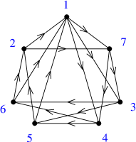
Figure 2: Quiver for $(P)dP_{4}$ theories.

Instead if we choose as a Kähler basis of the CY a surface obtained by blowing up $\mathbb{P}^{2}$ at non generic points it is possible to preserve more symmetries. A possible example with isometry $T^{3}$ is the toric CY described by the toric diagram with vertices $V_{i}=(x_{i},y_{i},1)$:

$$(0,0,1)\quad(1,0,1)\quad(2,0,1)\quad(2,1,1)\quad(1,2,1)\quad(0,2,1)\quad(0,1,1)$$ (5.1)

We will refer to this manifold as the complex cone over Pseudo del Pezzo 4, $PdP_{4}$, as already done in the literature. We draw the toric diagram in Figure 3 where we report also the dimer of the dual gauge theory. The dimer has $F=7$ gauge groups, $E=15$ chiral fields and $V=8$ superpotential terms.

Interestingly the quiver diagram of $PdP_{4}$ theory obtained from the dimer is just the same as the quiver of $dP_{4}$ theory in Figure 2: the difference between the two gauge theories is in the superpotential. They have the same global baryonic symmetries (equal to $d-3=4$ with $d$ the perimeter of the toric diagram), since they depend only on the quiver diagram and not on the superpotential (the total charge of every vertex and of every closed loop in the quiver is zero for baryonic symmetries). But for $PdP_{4}$ the superpotential allows two flavor symmetries, whereas for $dP_{4}$ new terms in the superpotential are added to break both the original flavor symmetries. As we will see we can interpret $dP_{4}$ theory as a “quotient” of $PdP_{4}$ in the sense of the previous Section.

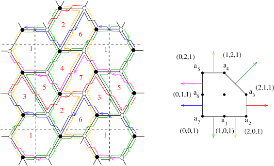
Figure 3: Dimer configuration and toric diagram for the toric $PdP_{4}$ theory.

5.1 The toric case

Let us start to study the toric theory. In Figure 3 we draw zig-zag paths in the dimer corresponding to vectors of the (p,q) web drawn in the same color; this correspondence allows to find the distribution of charges $a_{i}$ with the method explained in [21]:

$$\begin{array}[]{l@{\rightarrow}l@{\quad}l@{\rightarrow}l@{\quad}l@{\rightarrow}l}X_{17}&a_{1}+a_{6}+a_{7}&X_{21}&a_{7}&X_{27}&a_{3}+a_{4}\\ X_{73}&a_{2}&X_{14}&a_{1}+a_{2}+a_{3}&X_{74}&a_{5}\\ X_{13}&a_{4}+a_{5}+a_{6}&X_{62}&a_{5}+a_{6}&X_{51}&a_{4}+a_{5}\\ X_{61}&a_{2}+a_{3}&X_{52}&a_{1}+a_{2}&X_{36}&a_{1}+a_{7}\\ X_{45}&a_{6}+a_{7}&X_{46}&a_{4}&X_{35}&a_{3}\end{array}$$ (5.2)

where $X_{ij}$ is the chiral field from gauge group $i$ to $j$. The parameters $a_{i}$ are associated with vertices of the toric diagram as in Figure 3. If the sum $a_{1}+a_{2}+\ldots a_{7}$ is equal to 2 (0) we get a parametrization of non anomalous R-symmetries (global symmetries) in the toric theory.

We can start to study the closed loops in this quiver, independently from the superpotential. There are 24 irreducible (that cannot be written as a product of smaller loops) mesons:

$$\verb| |\begin{array}[]{c}\begin{array}[]{llll}m_{1}=X_{61}X_{17}X_{74}X_{46}&m_{3}=X_{21}X_{13}X_{35}X_{52}&m_{5}=X_{27}X_{73}X_{36}X_{62}&m_{7}=X_{14}X_{45}X_{51}\\ m_{2}=X_{51}X_{17}X_{73}X_{35}&m_{4}=X_{21}X_{14}X_{46}X_{62}&m_{6}=X_{27}X_{74}X_{45}X_{52}&m_{8}=X_{13}X_{36}X_{61}\\ \\ n_{1}=X_{21}X_{13}X_{36}X_{62}&n_{3}=X_{17}X_{74}X_{45}X_{51}&n_{5}=X_{27}X_{73}X_{35}X_{52}&n_{7}=X_{14}X_{46}X_{61}\\ n_{2}=X_{21}X_{14}X_{45}X_{52}&n_{4}=X_{17}X_{73}X_{36}X_{61}&n_{6}=X_{27}X_{74}X_{46}X_{62}&n_{8}=X_{13}X_{35}X_{51}\\ \\ \end{array}\\ \begin{array}[]{l@{\qquad}l}p_{1}=X_{21}X_{17}X_{74}X_{46}X_{62}&q_{1}=X_{21}X_{17}X_{74}X_{45}X_{52}\\ p_{2}=X_{21}X_{17}X_{73}X_{35}X_{52}&q_{2}=X_{21}X_{17}X_{73}X_{36}X_{62}\\ \end{array}\\[24.00006pt] \begin{array}[]{l@{\qquad}l}t_{1}=X_{27}X_{73}X_{35}X_{51}X_{14}X_{46}X_{62}&t_{2}=X_{27}X_{73}X_{36}X_{61}X_{14}X_{45}X_{52}\\ t_{3}=X_{27}X_{74}X_{45}X_{51}X_{13}X_{36}X_{62}&t_{4}=X_{27}X_{74}X_{46}X_{61}X_{13}X_{35}X_{52}\end{array}\end{array}$$ (5.3)

Since we are thinking to the abelianized theory with all $U(1)$ gauge groups we will not write traces in front of mesons.

From these definitions and from (5.2) we can deduce the parametrization of charges $\Psi$ for mesons, and setting the charge $\Psi$ equal to $\sum(\vec{m}\cdot\vec{V}_{i})\,a_{i}$ as in (4.1) we can see to which point $\vec{m}$ of $\mathcal{C}^{*}$ each meson is mapped:

$$\begin{array}[]{lll@{\qquad}lll}m_{1},\ldots m_{8}&\rightarrow&(0,0,1)&q_{1},q_{2}&\rightarrow&(-1,-1,3)\\ n_{1},n_{3},p_{1}&\rightarrow&(-1,0,2)&n_{5},n_{7}&\rightarrow&(1,0,0)\\ n_{2},n_{4},p_{2}&\rightarrow&(0,-1,2)&n_{6},n_{8}&\rightarrow&(0,1,0)\\[2.39996pt] t_{1},t_{4}&\rightarrow&(1,1,0)&t_{2}&\rightarrow&(1,-1,2)\\ t_{3}&\rightarrow&(-1,1,2)&&&\end{array}$$ (5.4)

Mesons mapped to the same integer point in $\mathcal{C}^{*}$ are F-term equivalent in the toric theory: the multiplicities of integer points in $\mathcal{C}^{*}$ is equal to one in toric theories. A basis for the cone $\mathcal{C}^{*}$, dual to the cone $\mathcal{C}$ in (5.1) is given by the points:

$$(0,1,0)\quad(-1,0,2)\quad(-1,-1,3)\quad(0,-1,2)\quad(1,0,0)\quad(0,0,1)$$ (5.5)

where the first five vectors are the perpendiculars to the facets of $\mathcal{C}$ and we have to add also $(0,0,1)$ to have a basis over the positive integer numbers. Note that the inverse image of the six generators in (5.5) under $\Psi$-map consists only of irreducible loops in the quiver, since composite mesons are mapped to the sum of the points corresponding to their constituents. Instead the irreducible mesons $t_{1}$, $t_{2}$, $t_{3}$ and $t_{4}$ are mapped to points in $\mathcal{C}^{*}$ that are not generators.

The superpotential for the toric theory can be read off from the dimer and it can be written as:

$$W_{T^{3}}=\sum_{i=1}^{8}c_{i}m_{i}$$ (5.6)

Recall in fact that in the toric superpotential there appear only mesons mapped to $\vec{m}_{0}=(0,0,1)$. We have also inserted general coefficients in front of every meson $c_{i}$, $i=1,\ldots 8$. Many of them can be reabsorbed with a rescaling of fields: $X_{ij}\rightarrow r_{ij}X_{ij}$, under which also mesons are rescaled as $m_{i}\rightarrow r_{i}m_{i}$ where the $r_{i}$ are products of the suitable $r_{ij}$. In the space of mesons $m_{1},\ldots m_{8}$ there is only one relation following from the definitions (5.3):

$$m_{1}m_{3}m_{5}m_{7}=m_{2}m_{4}m_{6}m_{8}\quad\textrm{or}:\quad r_{1}r_{3}r_{5}r_{7}=r_{2}r_{4}r_{6}r_{8}$$ (5.7)

This equality implies that the ratio:

$$\frac{c_{1}c_{3}c_{5}c_{7}}{c_{2}c_{4}c_{6}c_{8}}$$ (5.8)

is constant under field rescaling. Therefore since we have 8 coefficients in the superpotential (5.6) and one relation (5.7) we can reabsorb only 7 parameters in the superpotential through rescaling. For instance we can put the superpotential in the form:

$$W_{T^{3}}=m_{1}+m_{3}+m_{5}+m_{7}-b\left(m_{2}+m_{4}+m_{6}+m_{8}\right)$$ (5.9)

where we are assuming that all the original coefficients $c_{i}$ are different from zero.

Now we have also to impose the F-term constraints: by solving the F-term equations of (5.9) it is easy to see that there exists a complex three dimensional moduli space of vacua only if the ratio in (5.8) is equal to one, that is $b^{4}=1$. Of course any quartic root of unity is equivalent, up to rescaling. With the choice $b=1$ we find the usual result:

$$W_{T^{3}}=m_{1}+m_{3}+m_{5}+m_{7}-\left(m_{2}+m_{4}+m_{6}+m_{8}\right)$$ (5.10)

In fact $m_{1}$, $m_{3}$, $m_{5}$, $m_{7}$ correspond to white vertices in the dimer, whereas $m_{2}$, $m_{4}$, $m_{6}$, $m_{8}$ correspond to black vertices. The analysis performed here is general for toric theories: all but one coefficients in the superpotential can be reabsorbed through rescaling, and F-term conditions imply that also the last parameter is fixed as in (5.10) if we want a three dimensional moduli space. In fact we expect that for all toric three dimensional cones there are no complex structure deformations that leave the manifold a complex cone. If $b^{4}\neq 1$ in (5.9) indeed the dimension of the moduli space is reduced (there are one complex dimensional lines): this is a beta deformation of the toric theory [42].

5.2 $T^{1}$ and $T^{2}$ examples

Now we are ready to modify the toric theory as explained in Section 4. We observe in fact that to obtain the gauge theory for $dP_{4}$ we have to add to the superpotential mesons mapped to points $\vec{m}_{0}+k\,\vec{d}_{1}+h\,\vec{d}_{2}$ of the toric $\mathcal{C}^{*}$ with:

$$\vec{d}_{1}=(1,0,-1)\qquad\vec{d}_{2}=(0,1,-1)$$ (5.11)

The vectors $\vec{m}_{0}+k\,\vec{d}_{1}+h\,\vec{d}_{2}$ with $k$ and $h$ integers and belonging to $\mathcal{C}^{*}$ are exactly the generators of $\mathcal{C}^{*}$ in (5.5), therefore the superpotential becomes:

$$W_{T^{1}}=\sum_{i=1}^{8}a_{i}m_{i}+\sum_{i=1}^{8}c_{i}n_{i}+\sum_{i=1}^{2}\left(f_{i}p_{i}+g_{i}q_{i}\right)$$ (5.12)

that is we can consider all the first 20 mesons in (5.3), multiplied with generic coefficients $a_{i}$, $c_{i}$, $f_{i}$, $g_{i}$; for simplicity we will consider the coefficients $a_{i}$ of the toric terms different from zero. A particular choice of these coefficients reproduces the theory for $dP_{4}$ [27]. In fact we can study the superpotential (5.12) performing the same analysis just explained in the toric case: solving F-term equations and imposing the existence of a three-dimensional moduli space we get some equations for the coefficients $a_{i}$, $c_{i}$, $f_{i}$, $g_{i}$. We have not studied in detail all the possible branches of relations between these coefficients, but we have explicitly verified that there are solutions admitting a three dimensional cone of moduli space where the D3-branes can move. The isometry for the non toric cone is $T^{1}$ (it is enough that a suitable number of coefficients in (5.12) is different from zero, so that both original flavor symmetries are broken). Once we have imposed that the moduli space is a three dimensional complex cone, we have to remind that not all different choices of coefficients in the superpotential (5.12) determine inequivalent cones from the complex structure point of view. The computation of the complex deformations of the non toric cone is non trivial. In fact, differently from the toric case, non toric cones may admit complex structure deformations that leave the manifold a cone. One way to compute the deformations is to write the complex cone as an intersection in some $\mathbb{C}^{k}$ space, where typically the complex variables are associated with mesons, and then consider generic linear redefinitions of the complex variables. We have not performed explicitly the computation in the $T^{1}$ case starting with generic coefficients in the superpotential (5.12), however in this case by simple geometrical considerations we expect that there does not exist any complex structure deformation for the $T^{1}$ cone that leaves it a cone.

With the same quiver, we can build gauge theories whose moduli space is a non toric cone with isometry $T^{2}$: we can choose to project the toric theory only along one direction in (5.11), for instance choose:

$$\vec{d}=\vec{d}_{1}=(1,0,-1)$$ (5.13)

The points in $\mathcal{C}^{*}$ of the form $\vec{m}_{0}+k\,\vec{d}$ are: $(-1,0,2)$, $(0,0,1)$, $(1,0,0)$ for the integers $k=-1,0,1$ respectively; the corresponding superpotential is:

$$W_{T^{2}}=\sum_{i=1}^{8}a_{i}m_{i}+c_{1}n_{1}+c_{3}n_{3}+c_{5}n_{5}+c_{7}n_{7}+f_{1}p_{1}$$ (5.14)

Again it is simple to verify that there are choices of the coefficients $a_{i}$, $c_{i}$, $f_{1}$ for which there exists a three dimensional moduli space for the gauge theory with isometry $T^{2}$. Moreover in this $T^{2}$ case we explicitly checked that there are choices of parameters that give a one complex dimensional family of complex structure deformations that leave the manifold a cone. As we will see all the cones in this family of complex structure deformations have the same volume (for a Sasaki-Einstein metric on their basis) and the same multiplicities for holomorphic functions. In fact these features can be reconstructed from the original toric theory and from the information about the quotient (5.13). For more details about the moduli spaces of $(P)dP_{4}$ theories see Appendix B.

5.3 The cone of holomorphic functions

As explained in Section 4, it is easy to compute the possible charges of holomorphic functions and the multiplicities (that is the dimension of the vector space of holomorphic functions with an assigned charge), by taking the quotient of the toric $\mathcal{C}^{*}$ along the directions $\vec{d}_{1},\vec{d_{2}}$ for $T^{1}$ theory or along $\vec{d}$ for $T^{2}$. Let us first of all find an $SL(3,\mathbb{Z})$ transformation $A$ that sends the vector $\vec{d}_{1}$, $\vec{d_{2}}$ into $(1,0,0)$ $(0,1,0)$ respectively; choose for example:

$$A=\left(\begin{array}[]{lll}1&0&0\\ 1&2&1\\ 1&1&1\end{array}\right)\qquad\quad\vec{d}^{\,\,{}^{\prime}}_{1}=A\vec{d}_{1}=\left(\begin{array}[]{l}1\\ 0\\ 0\end{array}\right),\quad\vec{d}^{\,\,{}^{\prime}}_{2}=A\vec{d}_{2}=\left(\begin{array}[]{l}0\\ 1\\ 0\end{array}\right)$$ (5.15)

In this new system of coordinates the generating vectors (5.5) of the toric $\mathcal{C}^{*}$ are sent respectively into:

$$(0,2,1)\quad(-1,1,1)\quad(-1,0,1)\quad(0,0,1)\quad(1,1,1)\quad(0,1,1)$$ (5.16)

and the $\Psi$-map (LABEL:map) for the first 20 mesons in (5.3) becomes:

$$\begin{array}[]{lll@{\qquad}lll}m_{1},\ldots m_{8}&\rightarrow&(0,1,1)&q_{1},q_{2}&\rightarrow&(-1,0,1)\\ n_{1},n_{3},p_{1}&\rightarrow&(-1,1,1)&n_{5},n_{7}&\rightarrow&(1,1,1)\\ n_{2},n_{4},p_{2}&\rightarrow&(0,0,1)&n_{6},n_{8}&\rightarrow&(0,2,1)\end{array}$$ (5.17)

Now the quotient along the direction $\vec{d}^{\,\,{}^{\prime}}=\vec{d}^{\,\,{}^{\prime}}_{1}$ is simply the projection of the cone $\mathcal{C}^{*}$ on the plane $(y^{\prime},z^{\prime})$; we draw it in Figure 4a). This is the cone of charges for the theories with isometry $T^{2}$ (5.14); the multiplicities of holomorphic functions with charge $(n^{\prime},m^{\prime})$ are the number of points of $\mathcal{C}^{*}$ projected to $(n^{\prime},m^{\prime})$. For example among the generators (5.16), the two vectors (-1,0,1), (0,0,1) are mapped into (0,1); the three vectors (-1,1,1), (1,1,1), (0,1,1) are mapped into (1,1) and the vector (0,2,1) is mapped into (2,1).

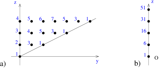
Figure 4: The multiplicities of holomorphic functions with fixed charge(s) over $(P)dP_{4}$ cones with a) isometry $T^{2}$, b) isometry $T^{1}$.

In the same way one can obtain the cone (indeed a half-line) of charges of holomorphic functions for the theories with isometry $T^{1}$ (5.12) by projecting the toric $\mathcal{C}^{*}$ on the axis $z^{\prime}$; we draw it in Figure 4b). All the generators (5.16) are mapped into the point 1, which has therefore multiplicity equal to 6.

We can perform some checks that the cones of holomorphic functions are those drawn in Figures 4 by writing down the linear relations among mesons induced by F-term relations in the different theories and counting the number of linearly independent mesons with a fixed charge. We will do that for mesons mapped to the generators of $\mathcal{C}^{*}$, one should check the multiplicities also for more complicated mesons. Linear relations among mesons are obtained by multiplying the F-term relation $\partial W/\partial X_{ij}=0$ with paths going from node $i$ to node $j$. For example $X_{ij}\partial W/\partial X_{ij}=0$ can be rewritten in terms of mesons appearing in the superpotential; other linear relations can be deduced manipulating non linear equations between mesons using these linear constraints.

In the toric case (5.10) the linear relations are simple equalities; for the first 20 generators in (5.3) we get:

$$\begin{array}[]{l@{\qquad}l}m_{1}=\ldots=m_{8}&q_{1}=q_{2}\\ n_{1}=n_{3}=p_{1}&n_{5}=n_{7}\\ n_{2}=n_{4}=p_{2}&n_{6}=n_{8}\end{array}$$ (5.18)

More generally in toric theories mesons mapped to the same point in $\mathcal{C}^{*}$ are equal, so that the cone of charges of holomorphic functions is $\mathcal{C}^{*}$ and each integer point in $\mathcal{C}^{*}$ has multiplicity equal to one.

Consider instead the theory $T^{2}$ (5.14) and rescale the coefficients in the superpotential to the form:

$$W=a(m_{1}+m_{3}+m_{5}+m_{7})-b(m_{2}+m_{4}+m_{6}+m_{8})+cn_{1}-dn_{3}+en_{5}-fn_{7}+gp_{1}$$ (5.19)

The 13 mesons $m_{1}\ldots m_{8}$, $n_{1}$, $n_{3}$, $p_{1}$, $n_{5}$, $n_{7}$, that are all mapped to the point $(1,1)$, satisfy a set of 10 independent linear relations:

$$\begin{array}[]{lll}am_{1}-bm_{2}-dn_{3}+gp_{1}=0&am_{3}-bm_{4}+cn_{1}+gp_{1}=0&am_{5}-bm_{6}+en_{5}=0\\ -bm_{2}+am_{5}+en_{5}=0&-bm_{4}+am_{7}-fn_{7}=0&am_{3}-bm_{8}+cn_{1}=0\\ -bm_{4}+am_{5}+cn_{1}+gp_{1}=0&-bm_{2}+am_{7}-dn_{3}=0&-fm_{1}+an_{3}-bp_{1}=0\\ -fm_{4}-bn_{1}+ap_{1}=0&&\end{array}$$ (5.20)

so that we have verified that there are 3 independent holomorphic functions with charge $(1,1)$. The 5 mesons $n_{2}$, $n_{4}$, $p_{2}$, $q_{1}$, $q_{2}$, that are mapped to the point $(0,1)$ satisfy 3 independent linear relations:

$$\begin{array}[]{lll}ap_{2}-bn_{4}+cq_{2}=0&an_{2}-bp_{2}-dq_{1}&ep_{2}-bq_{1}+aq_{2}=0\end{array}$$ (5.21)

so that the point $(0,1)$ has multiplicity 2. The mesons $n_{6}$, $n_{8}$, mapped to $(2,1)$, satisfy one linear relation:

$$\left(a^{2}-df\right)n_{6}-b^{2}n_{8}=0$$ (5.22)

and therefore the point $(2,1)$ has multiplicity 1. Note that all relations written for the theory $T^{2}$ reduce to equalities in (5.18) if we set $c=d=e=f=g=0$, and $a=b=1$, that is when we recover the toric superpotential. Note that obviously both in the toric theory $T^{3}$ and in the $T^{2}$ theory there are linear relations only for mesons having the same global charges. The introduction of superpotential terms that break one flavor symmetry modifies the linear relations of the toric case: now all mesons mapped to aligned integer points $\vec{m}+k\vec{d}$ of the toric $\mathcal{C}^{*}$ may appear in the same linear relations since they have the same charges in the $T^{2}$ theory (4.5).

The case of the theories with symmetry $T^{1}$ is completely analogous: linear relations written before (LABEL:lineart21), (5.21), (5.22) are extended to include all the 20 considered mesons, that are now mapped to the same point 1 in Figure 4b); this point has therefore multiplicity equal to 6.

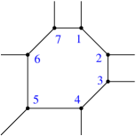
Figure 5: Resolution of complex cone over $PdP_{4}$

5.4 Characters and volumes

The equivariant index of the Cauchy-Riemann operator $\bar{\partial}$ [45] on a (CY) cone allows to count the number $c_{m}$ of holomorphic functions with fixed charge $m\equiv(m_{1},\ldots,m_{r})$ [15], where $r$ is the dimension of the maximal torus $T^{r}$ of the isometry group (in our examples $r=1,2$ or $3$). The character $C(q)$, $q\equiv(q_{1},\ldots q_{r})$ is the generating function of the number of holomorphic functions:

$$C(q)=\sum c_{m}\,q^{m}\equiv\sum c_{m}\,q_{1}^{m_{1}}\ldots q_{r}^{m_{r}}$$ (5.23)

For toric cones holomorphic functions are in one to one correspondence with the set $\mathcal{S}_{C}$ of integer points of $\mathcal{C}^{*}$, and hence the character is:

$$C(q)=\sum_{m\in\mathcal{S}_{C}}q^{m}$$ (5.24)

moreover it can be easily computed by resolving the cone [15]: the contributions to $C(q)$ come only from the fixed points of the toric action.

In our example we can choose for $PdP_{4}$ the resolution drawn in Figure 5 with fixed points $p_{A}$, $A=1,\ldots 7$; at each fixed point $A$ there are $n=3$ primitive edge vectors $u_{i}^{(A)}$, $i=1,2,3$ (in the coordinates where the generators are (5.5)):

$$\begin{array}[]{llll}p_{1}:&u_{1}^{(1)}=(0,1,0)&u_{2}^{(1)}=(-1,0,1)&u_{3}^{(1)}=(1,-1,0)\\ p_{2}:&u_{1}^{(2)}=(1,0,0)&u_{2}^{(2)}=(0,-1,1)&u_{3}^{(2)}=(-1,1,0)\\ p_{3}:&u_{1}^{(3)}=(1,0,0)&u_{2}^{(3)}=(0,1,-1)&u_{3}^{(3)}=(-1,-1,2)\\ p_{4}:&u_{1}^{(4)}=(0,-1,2)&u_{2}^{(4)}=(-1,0,1)&u_{3}^{(4)}=(1,1,-2)\\ p_{5}:&u_{1}^{(5)}=(-1,-1,3)&u_{2}^{(5)}=(1,0,-1)&u_{3}^{(5)}=(0,1,-1)\\ p_{6}:&u_{1}^{(6)}=(-1,0,2)&u_{2}^{(6)}=(1,1,-2)&u_{3}^{(6)}=(0,-1,1)\\ p_{7}:&u_{1}^{(7)}=(0,1,0)&u_{2}^{(7)}=(-1,-1,2)&u_{3}^{(7)}=(1,0,-1)\\ \end{array}$$ (5.25)

Then the character of the $PdP_{4}$ theory can be computed using the general formula for toric cones [15]:

$$C_{T^{3}}(q)=\sum_{p_{A}}\prod_{i=1}^{3}\frac{1}{1-q^{\,u_{i}^{(A)}}}$$ (5.26)

where again for the vectors $q$, $u$, the expression $q^{u}$ stands for: $q_{1}^{u_{1}}q_{2}^{u_{2}}q_{3}^{u_{3}}$.

We perform the change of coordinates in (5.15) and apply equation (5.26) after transforming vectors in (LABEL:uvec), that is with the replacement $u_{i}^{(A)}\rightarrow A\,u_{i}^{(A)}$; after some simplifications we get:

$$C_{T^{3}}(q)=\frac{q_{1}\left(q_{2}\left(-q_{2}^{2}q_{3}^{2}-q_{2}q_{3}+q_{2}+1\right)q_{3}^{2}+q_{1}\left(q_{2}^{2}q_{3}^{2}+q_{2}(q_{3}-1)q_{3}-1\right)\right)}{(q_{1}-q_{3})(q_{3}-1)\left(q_{2}^{2}q_{3}-1\right)\left(q_{2}q_{3}q_{1}^{2}-\left(q_{2}^{2}q_{3}^{2}+1\right)q_{1}+q_{2}q_{3}\right)}$$ (5.27)

The cone of holomorphic functions for the theory $T^{2}$ is obtained by projecting the toric cone $\mathcal{C}^{*}$ along the direction $\vec{d}^{\,\,{}^{\prime}}=(1,0,0)$; therefore the character $C_{T^{2}}(q)$ for $T^{2}$ theories, $q=(q_{2},q_{3})$, is obtained simply by setting $q_{1}=1$ in equation (5.27), this is evident from the expansions in (5.24). We obtain:

$$C_{T^{2}}(q)=\frac{-q_{2}^{2}q_{3}^{3}-2q_{2}(q_{3}-1)q_{3}+1}{(q_{3}-1)^{2}(q_{2}q_{3}-1)\left(q_{2}^{2}q_{3}-1\right)}$$ (5.28)

and this is the generating function for Figure 4a).

Analogously the character $C_{T^{1}}(q)$ for the theory $T^{1}$, $q=q_{3}$, is obtained by setting $q_{1}=1$ and $q_{2}=1$, since now the cone of charges for holomorphic functions is obtained by projecting the toric $\mathcal{C}^{*}$ along the plane generated by $\vec{d}^{\,\,{}^{\prime}}_{1}=(1,0,0)$ and $\vec{d}^{\,\,{}^{\prime}}_{2}=(0,1,0)$. We obtain:

$$C_{T^{1}}(q)=\frac{q_{3}^{2}+3q_{3}+1}{(1-q_{3})^{3}}$$ (5.29)

and this is the generating function for Figure 4b).

Remarkably in [15] it was shown that the volume of a Sasaki metric over the base of the cone depends only on the Reeb vector $b=(b_{1},\ldots b_{r})$, and can be expressed in terms of contributions localized on the vanishing locus of the Reeb vector field; comparing their formula for the volume with that of the equivariant index for the character, the authors of [15] proved the interesting relation:

$$V(b)=\lim_{t\rightarrow 0}t^{n}C(e^{-tb})$$ (5.30)

where in our case $n=3$ is the complex dimension of the cone over the Sasaki manifold; the character is evaluated in $q=e^{-tb}$ defined as $q_{i}=e^{-tb_{i}}$. The function $V(b)$ is the normalized volume function for the Sasaki manifold:

$$V(b)\equiv\frac{\textrm{Vol}(b)}{\textrm{Vol}(S^{2n-1})}\qquad\qquad\textrm{for}\,\,\,n=3:\,\,\,V(b)=\frac{\textrm{Vol}(b)}{\pi^{3}}$$ (5.31)

For toric manifolds the limit in (5.30) applied to (5.26) yields:

$$V(b)=\sum_{p_{A}}\prod_{i=1}^{3}\frac{1}{(b,u_{i}^{\,(A)})}$$ (5.32)

In our examples, performing the limit (5.30) for equations (5.27), (5.28), (5.29) we obtain:

$$V_{T^{3}}(b) = \displaystyle\frac{2b_{2}^{2}+7b_{3}b_{2}+5b_{3}^{2}-b_{1}(2b_{2}+3b_{3})}{(b_{1}-b_{3})b_{3}(2b_{2}+b_{3})\left(b_{1}^{2}-(b_{2}+b_{3})^{2}\right)}$$

$$V_{T^{2}}(b) = \displaystyle\frac{2b_{2}+5b_{3}}{b_{3}^{2}(b_{2}+b_{3})(2b_{2}+b_{3})}$$

$$V_{T^{1}}(b) = \displaystyle\frac{5}{b_{3}^{3}}$$ (5.33)

These are the formulas for the normalized volume of a Sasaki metric of Reeb vector $b$ over the basis of the cones we are considering. Note that $V_{T^{2}}(b)$ is obtained from $V_{T^{3}}(b)$ by setting $b_{1}=0$: in fact $q_{1}=e^{-tb_{1}}$ and $q_{1}=1$ to obtain the $T^{2}$ theory. In the same way $V_{T^{1}}(b)$ is obtained by setting $b_{1}=b_{2}=0$ in $V_{T^{3}}(b)$.

We should try to find the position of the Reeb vector corresponding to a Sasaki-Einstein metric to compute the volume in this case. Indeed the Reeb vector of a Sasaki-Einstein metric is at the minimum of the functions $V_{T^{r}}$ restricted to a suitable affine space of dimension $r-1$ [15], and $b$ inside the direct cone (the dual of the image of the momentum map). For toric cases [14] this is the plane $z=3$ in coordinates (5.1); in our basis (5.33) this plane becomes: $b_{2}+b_{3}=3$. The Z-minimization for the toric case leads to: $\vec{b}=(-0.37908,-0.37908,3.37908)$. In non toric theories the affine space where to perform the volume minimization is not explicitly known; therefore in our examples we will extract the position of the Reeb vector for Sasaki-Einstein metrics from the gauge theory, studying the scaling dimensions of mesons.

5.5 Central and R-charges

In all kinds of theories $T^{1}$, $T^{2}$, $T^{3}$ we are considering, the trial R-charges for chiral fields can be parametrized with the $a_{i}$, $i=1,\ldots 7$, associated with vertices of the toric diagram (Figure 3) as in (5.2), but we have to impose more linear constraints on them as the number of symmetries decreases. In fact condition (4.2) must always be imposed in all cases $T^{1}$, $T^{2}$, $T^{3}$:

$$a_{1}+a_{2}+a_{3}+a_{4}+a_{5}+a_{6}+a_{7}=2$$ (5.34)

If the isometry is $T^{2}$ we have the further constraint (4.5), which in our case is:

$$a_{2}+a_{3}-a_{5}-a_{6}-a_{7}=0$$ (5.35)

and if the isometry is $T^{1}$ there are two linear constraints (4.6), which in our example are:

$$\begin{array}[]{l}a_{2}+a_{3}-a_{5}-a_{6}-a_{7}=0\\ -a_{1}-a_{2}+a_{4}+a_{5}-a_{7}=0\end{array}$$ (5.36)

The trial central charge $a$ can be written as:

$$\begin{array}[]{lll}a&=&\frac{9}{32}\textrm{tr}\,R^{3}=\frac{9}{32}\left[7+\left(a_{1}+a_{6}+a_{7}-1\right)^{3}+\left(a_{7}-1\right)^{3}+\left(a_{3}+a_{4}-1\right)^{3}+\left(a_{2}-1\right)^{3}\right.\\ &&+\left(a_{1}+a_{2}+a_{3}-1\right)^{3}+\left(a_{5}-1\right)^{3}+\left(a_{4}+a_{5}+a_{6}-1\right)^{3}+\left(a_{5}+a_{6}-1\right)^{3}\\ &&+\left(a_{4}+a_{5}-1\right)^{3}+\left(a_{2}+a_{3}-1\right)^{3}+\left(a_{1}+a_{2}-1\right)^{3}+\left(a_{1}+a_{7}-1\right)^{3}\\ &&+\left(a_{6}+a_{7}-1\right)^{3}+\left(a_{4}-1\right)^{3}+\left(a_{3}-1\right)^{3}\left.\right]\end{array}$$ (5.37)

where we have used (5.2) for the chiral fields. Note moreover that the trace of the trial R-symmetry is zero $\textrm{tr}\,R=0$ in all (non) toric theories built modifying toric theories as in Section 4. The proof is the same as in toric theories [20], since the chiral field content and relation (4.2) are the same also in the modified non toric theories.

Now we can perform a-maximization [13] and find exact R-charges; the maximization of (5.37) is performed on an affine space of dimension 6 for our $T^{3}$ theory, of dimension 5 for the $T^{2}$ theories and of dimension 4 for the $T^{1}$ theories. The results are:

$$\begin{array}[]{l}\begin{array}[]{lllll}\textrm{case}\,\,T^{3}:&a_{2}=a_{5}\simeq 0.42698&a_{3}=a_{4}\simeq 0.29777&a_{7}\simeq 0.55049&a_{1}=a_{6}=0\\[18.00005pt] \textrm{case}\,\,T^{2}:&a_{2}=a_{7}=\displaystyle\frac{2}{3}(\sqrt{3}-1)&a_{3}=a_{5}=\displaystyle\frac{4}{3}(2-\sqrt{3})&a_{4}=\displaystyle\frac{4}{\sqrt{3}}-2&a_{1}=a_{6}=0\end{array}\\[30.00008pt] \,\,\,\textrm{case}\,\,T^{1}:\,\,\,\,a_{2}=a_{3}=a_{4}=a_{5}=a_{7}=\displaystyle\frac{2}{5}\,\,\,\,\,\,\,a_{1}=a_{6}=0\end{array}$$ (5.38)

and the values of central charges $a$ for the different theories are:

$$a_{T^{3}}=1.41805\qquad a_{T^{2}}=6\sqrt{3}-9\qquad a_{T^{1}}=\frac{27}{20}$$ (5.39)

Using the values above we can compute the exact R-charges $R$ of mesons and hence the scaling dimensions $\Delta=3/2R$, which can be also expressed through the Reeb vector $\vec{b}$ of a Sasaki-Einstein metrics: $\Delta=\vec{b}\cdot\vec{m}$. Considering the mesons mapped to generators $\vec{m}$ of the cone of charges for holomorphic functions, we are able to find the Reeb vector corresponding to a Sasaki-Einstein metric. The results, in the same coordinate system of (5.33) are:

$$\begin{array}[]{ll}\textrm{case}\,\,T^{3}:&\vec{b}=(b_{1},b_{2},b_{3})=(-0.37908,-0.37908,3.37908)\\ \textrm{case}\,\,T^{2}:&\vec{b}=(b_{2},b_{3})=(3-2\sqrt{3},2\sqrt{3})\\ \textrm{case}\,\,T^{1}:&\vec{b}=b_{3}=3\\ \end{array}$$ (5.40)

Note that in the toric case the Reeb vector lies in the plane $b_{2}+b_{3}=3$ as expected and the result here agrees with that of Z-minimization, as already proved in the general toric case. The case $T^{2}$ is less trivial since we have three generators of the cone of charges: $\vec{m}=(0,1)$, $\vec{m}=(1,1)$ and $\vec{m}=(2,1)$. The three equations $\Delta=\vec{m}\cdot\vec{b}$ in the case $T^{2}$ are respectively:

$$b_{3}=2\sqrt{3}\qquad\quad b_{2}+b_{3}=3\qquad\quad 2b_{2}+b_{3}=6-2\sqrt{3}$$ (5.41)

This system in two unknowns is indeed consistent and the solution is in (5.40).

Inserting the values for the Reeb vectors (5.40) into the expressions for the volumes (5.33) we are able to find the normalized volumes of the basis of the CY cones:

$$V_{T^{3}}=0.176299\qquad V_{T^{2}}=\frac{3+2\sqrt{3}}{36}\qquad V_{T^{1}}=\frac{5}{27}$$ (5.42)

Note that our methods allow to compute the volumes also for non complete intersections. Now it is possible to compare these volumes with the values for the central charge $a$ (5.39); according to AdS/CFT predictions the following relation must hold:

$$a=\frac{\pi^{3}}{4\textrm{Vol}}=\frac{1}{4V}$$ (5.43)

and it is easy to check that (5.39) match (5.42) in all three cases $T^{3}$, $T^{2}$ and $T^{1}$. A general proof of this matching for toric theories was given in [20]; in Section 8 we will give a simple proof of (5.43) for the class of non toric theories obtained by modifying toric theories as in Section 4.

6 Generalized conifolds of type $A_{k}$

In this Section we apply the ideas of Section 4 to another non-toric theory already known in the literature [47, 46], that we will call generalized conifold of type $A_{2}$. This theory is part of a big family of $\mathcal{N}=1$ superconformal quiver gauge theories that are infrared fixed points of the renormalization group flow induced by deforming $ADE$ $\mathcal{N}=2$ superconformal field theories by mass terms for the adjoint chiral fields [47, 46]. We will extend our analysis also to the generalized conifolds of type $A_{k}$.

The generalized conifold of type $A_{2}$ is the $\mathcal{N}=1$ superconformal quiver gauge theory that lives on a stack of $N$ parallel $D3$-branes at the singular point of a type $D_{4}$ complex three-fold [48]:

$$x^{3}+y^{2}x=zw$$ (6.1)

The theory has the gauge group $SU(N)\times SU(N)\times SU(N)$ and six chiral matter fields $A$, $\tilde{A}$, $B$, $\tilde{B}$, $C$, $\tilde{C}$ that transform under the gauge group as shown in Figure 6 [46].

Figure 6: The quiver of the generalized conifold of type $A_{2}$.

The superpotential is given by:

$$W=a_{1}^{2}\hbox{ Tr }(A\tilde{A})^{2}+a_{2}^{2}\hbox{ Tr }(B\tilde{B})^{2}+a_{3}^{2}\hbox{ Tr }(C\tilde{C})^{2}+$$

$$2a_{1}a_{3}\hbox{ Tr }A\tilde{A}\tilde{C}C+2a_{1}a_{2}\hbox{ Tr }B\tilde{B}\tilde{A}A+2a_{2}a_{3}\hbox{ Tr }C\tilde{C}\tilde{B}B$$ (6.2)

where $a_{1}$, $a_{2}$, $a_{3}$ are three independent coupling constants. To reconstruct the geometry from the field theory we reduce as usual to the abelian case in which the gauge group is $U(1)^{3}$ and we define the following gauge invariants:

$$x_{1}=A\tilde{A},\quad x_{2}=B\tilde{B},\quad x_{3}=C\tilde{C}$$

$$z=ABC\quad w=\tilde{A}\tilde{B}\tilde{C}$$ (6.3)

These variables are subject to the constraint:

$$x_{1}x_{2}x_{3}=zw$$ (6.4)

and in term of these gauge invariants the superpotential (6) can be written as

$$W=(a_{1}x_{1}+a_{2}x_{2}+a_{3}x_{3})^{2}$$ (6.5)

The $F$-term equations reduce to the linear constraint: $a_{1}x_{1}+a_{2}x_{2}+a_{3}x_{3}=0$, hence we can use $x_{1}$, $x_{2}$, $z$, $w$ as the generators of the mesonic chiral ring and equation (6.4) becomes, after fields rescaling, $x_{1}x_{2}(x_{1}+x_{2})=zw$. This is equivalent to the cone in (6.1) after the complex variables redefinitions: $x_{1}=(x+iy)/\sqrt[3]{2}$, $x_{2}=(x-iy)/\sqrt[3]{2}$. In this way the field theory reconstructs the geometry along its Higgs branch [46].

This theory is important for our task because it is the gauge theory dual to a non-toric geometry. If we give arbitrary weights under a $\mathbb{C}^{*}$ action to the four embedding variables of the singularity it is easy to show that equation (6.1) admits only two independent actions. This imply that the variety is of type $T^{2}$. The field theory has indeed only two non-anomalous $U(1)$ symmetries that are of non-baryonic type [46] and they correspond to the imaginary part of the $\mathbb{C}^{*}$ action; these symmetries can be organized as the $R$-symmetry $U(1)_{R}$ and the flavor symmetry $U(1)_{F}$:

$$\begin{array}[]{l|llllll}&A&\tilde{A}&B&\tilde{B}&C&\tilde{C}\\ \hline\cr U(1)_{R}&1/2&1/2&1/2&1/2&1/2&1/2\\[6.00002pt] U(1)_{F}&1&-1&0&0&0&0\end{array}$$ (6.6)

The quiver gauge theory we have just discussed is the smallest one of the infinite family of generalized conifolds of type $A_{k-1}$ [47, 46]. The quivers of these theories can be obtained from the associated affine Dinkin diagrams of the $A_{k-1}$ orbifold singularities by deleting the arrows of the adjoint chiral superfields: there are $k$ $SU(N)$ gauge groups labeled by a periodic index $i=1,\ldots k$ and $2k$ chiral superfields, divided in the two sets $X_{i}$, and $\tilde{X}_{i}$. The chiral field $X_{i}$ goes from node $i$ to $i+1$; instead $\tilde{X}_{i}$ goes from node $i+1$ to node $i$. The quiver in Figure 6 corresponds to the case $k=3$. In the abelian case the theory has $U(1)^{k}$ gauge group and we can define the minimal set of gauge invariants:

$$x_{i}=X_{i}\tilde{X}_{i},\quad z=X_{1}X_{2}...X_{k},\quad w=\tilde{X_{1}}\tilde{X_{2}}...\tilde{X}_{k}.$$ (6.7)

These $k+2$ mesons satisfy the following relation:

$$x_{1}x_{2}...x_{k}=zw$$ (6.8)

The superpotential for these theories written in term of the above mesons is:

$$W=\sum_{i=1}^{k}(a_{i}x_{i}^{2}+2b_{i}x_{i}x_{i-1})$$ (6.9)

The study of the moduli space for these theories has already been performed in [46]: the F-term relations following from (6.9) reduce to the $k$ linear relations: $b_{i}x_{i-1}+a_{i}x_{i}+b_{i+1}x_{i+1}=0$. In order to have a three dimensional cone, we have to impose suitable relations on the parameters $a_{i}$, $b_{i}$ (see equation (4.8) in [46]) in the superpotential such that only $k-2$ of the F-term linear relations are independent: we can use them to express $x_{3}$, …$x_{k}$ as linear functions of $x_{1}$ and $x_{2}$. Hence relation (6.8) becomes, using also fields rescaling [46]:

$$x_{1}x_{2}(x_{1}+x_{2})\prod_{j=1}^{k-3}(x_{1}+\alpha_{j}x_{2})=zw$$ (6.10)

This equation in term of independent mesons $x_{1}$, $x_{2}$, $z$, $w$ expresses the three-dimensional cone as a complex submanifold in $\mathbb{C}^{4}$. The $\alpha_{j}$ in (6.10) cannot be reabsorbed into linear redefinitions of the variables and hence parametrize the complex structure deformations that leave the moduli space a cone.

Looking at the $\mathbb{C}^{*}$ action on the embedding variables one can show that the varieties (6.10) allow only a $(\mathbb{C}^{*})^{2}$ action. The superpotential of the theories (6.9) is a quartic polynomial in the elementary fields and, using the symmetries of the quiver gauge theory, we immediately find that the exact $R$-charges of the chiral superfields are all equal to $1/2$. Hence the results of a-maximization are simple:

$$\textrm{a-max:}\qquad R(X_{i})=R(\tilde{X}_{i})=\frac{1}{2}\qquad a=\frac{9}{32}\left[k+k(-\frac{1}{2})^{3}+k(-\frac{1}{2})^{3}\right]=\frac{27}{128}k$$ (6.11)

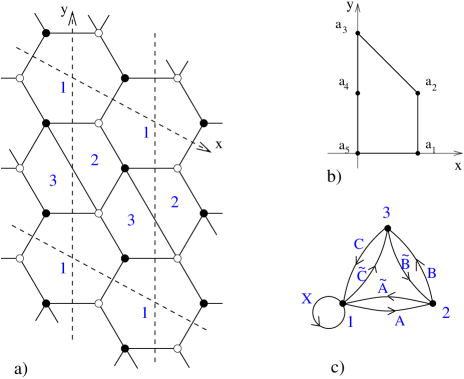
Figure 7: The SPP theory: a) dimer configuration b) toric diagram c) quiver diagram.

Interestingly the generalized conifolds of type $A_{k-1}$ belong to the class of non toric theories introduced in Section 4. Let us start with the case $k=3$; first of all we have to find a toric theory with a quiver that can be reduced to that of Figure 6: we can choose for instance the well know theory of the SPP, whose toric diagram $\mathcal{C}$ is:

$$(0,0,1)\quad(1,0,1)\quad(1,1,1)\quad(0,2,1)$$ (6.12)

The dimer, toric diagram and quiver are drawn in Figure 7. There are $F=3$ gauge groups, and $E=7$ chiral fields: there are all the fields appearing in the generalized $A_{2}$ conifold: $A$, $\tilde{A}$, $B$, $\tilde{B}$, $C$, $\tilde{C}$ plus an adjoint: $X_{11}\equiv X$, to which we will have to give mass. In the SPP quiver the minimal loops are the mesons in (6) plus the adjoint $X$. The toric superpotential can be written as:

$$W_{T^{3}}=x_{1}X+x_{2}x_{3}-x_{3}X-x_{1}x_{2}$$ (6.13)

The dual cone $\mathcal{C}^{*}$ has four generators over integer numbers:

$$(0,1,0)\quad(-1,0,1)\quad(-1,-1,2)\quad(1,0,0)$$ (6.14)

It is easy to find the $\Psi$-map for the generating mesons: $x_{1}$, $x_{2}$, $x_{3}$, $z$, $w$ and $X$:

$$\begin{array}[]{lll}\textrm{meson}&\textrm{charge}&\Psi\textrm{-map}\\ w&a_{2}+2a_{3}+a_{4}&(0,1,0)\\ x_{1},x_{3}&a_{3}+a_{4}+a_{5}&(-1,0,1)\\ z&a_{1}+a_{4}+2a_{5}&(-1,-1,2)\\ x_{2},X&a_{1}+a_{2}&(1,0,0)\end{array}$$ (6.15)

where the $a_{i}$ are associated with vertices of the toric diagram as in Figure 7b). From the above table it is immediate to see that we can choose as linearly independent mesons: $x_{1}$, $x_{2}$, $z$ and $w$ and that the SPP can be expressed in terms of this variables as the surface in $\mathbb{C}^{4}$: $x_{1}^{2}x_{2}=zw$, to be compared with the equation for the generalized conifold of type $A_{2}$ (6.10): $x_{1}^{2}x_{2}+x_{1}x_{2}^{2}=zw$. To modify the SPP superpotential and recover the generalized conifold of type $A_{2}$ we have to introduce the mass term $X^{2}$, which is mapped to the point of $\mathcal{C}^{*}$: $(2,0,0)$, as can be deduced from (6.15). We deduce that $\vec{d}=(2,0,0)-(0,0,1)=(2,0,-1)$, and that we can add to the superpotential all mesons that are mapped to the three points of $\mathcal{C}^{*}$: $(0,0,1)$, $(2,0,0)$, $(-2,0,2)$, that are all the points of $\mathcal{C}^{*}$ of the form: $\vec{m}_{0}+k\vec{d}$. The resulting modified superpotential is thus:

$$W_{T^{2}}=\left(x_{1}X+x_{2}x_{3}+x_{3}X+x_{1}x_{2}\right)+\left(x_{2}^{2}+X^{2}+x_{2}X\right)+\left(x_{1}^{2}+x_{3}^{2}+x_{1}x_{3}\right)$$ (6.16)

where in front of each term there is a generic coefficient that we have understood for simplicity. Integrating out the massive field $X$, one recovers the same superpotential of the generalized conifold of type $A_{2}$ (6.5). Therefore we have shown that this non toric theory can be obtained by quotienting SPP along $\vec{d}=(2,0,-1)$.

The character $C_{T^{3}}(q)$ for the SPP theory can be deduced easily from the general formula (5.26) [15] and using the following resolution of the SPP singularity:

$$\begin{array}[]{llll}p_{1}:&u_{1}^{(1)}=(0,1,0)&u_{2}^{(1)}=(1,0,0)&u_{3}^{(1)}=(-1,-1,1)\\ p_{2}:&u_{1}^{(2)}=(-1,0,1)&u_{2}^{(2)}=(0,-1,1)&u_{3}^{(2)}=(1,1,-1)\\ p_{3}:&u_{1}^{(3)}=(1,0,0)&u_{2}^{(3)}=(0,1,-1)&u_{3}^{(3)}=(-1,-1,2)\end{array}$$ (6.17)

which is shown in Figure 8a). But before computing the character we perform an $SL(3,\mathbb{Z})$ transformation $A$ that sends $\vec{d}\rightarrow(0,0,1)$; we can choose for instance:

$$A=\left(\begin{array}[]{lll}1&1&2\\ 1&0&2\\ 0&0&-1\end{array}\right)$$ (6.18)

with this change of coordinates the vectors of $\mathcal{C}^{*}$ (6.14) become respectively:

$$(1,0,0)\quad(1,1,-1)\quad(2,3,-2)\quad(1,1,0)$$ (6.19)

The cone $\mathcal{C}^{*}_{T^{2}}$ in this new system of coordinates is the projection of $\mathcal{C}^{*}$ (6.19) on the plane $(x,y)$, since now $\vec{d}=(0,0,1)$; we see therefore that $w$ is mapped to the point $(1,0)$, $z$ is mapped to $(2,3)$ and $x_{1}$, $x_{2}$, $x_{3}$ are mapped to $(1,1)$. The cone $\mathcal{C}^{*}_{T^{2}}$ for the generalized conifold of type $A_{2}$ is drawn in Figure 8b).

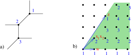
Figure 8: a) Resolution of the SPP singularity. b) $\mathcal{C}^{*}_{T^{2}}$ for the generalized conifold of type $A_{2}$ with multiplicities of holomorphic functions.

After applying the matrix $A$ (6.18) to the vectors $u_{i}$ in (6.17) we find the character for the SPP in the new system of coordinates :

$$C_{T^{3}}(q)=\frac{{q_{3}}^{3}-\left({q_{1}}^{3}\,{q_{2}}^{3}\,q_{3}\right)}{\left(1-q_{1}\right)\,\left(1-q_{1}\,q_{2}\right)\,\left(q_{1}\,q_{2}-q_{3}\right)\,\left({q_{1}}^{2}\,{q_{2}}^{3}-{q_{3}}^{2}\right)}$$ (6.20)

and the character for the generalized conifold of type $A_{2}$ is obtained by inserting $q_{3}=1$ in $C_{T^{3}}$, in order to count all the points of the toric $\mathcal{C}^{*}$ that are mapped to the same point in the plane $(x,y)$:

$$C_{T^{2}}(q)=\frac{1-{q_{1}}^{3}\,{q_{2}}^{3}}{\left(1-q_{1}\right)\,{\left(1-q_{1}\,q_{2}\right)}^{2}\,\left(1-{q_{1}}^{2}\,{q_{2}}^{3}\right)}$$ (6.21)

The function $C_{T^{2}}(q)$ generates the multiplicities that are reported in Figure 8b) and that can be computed directly in some simple cases in the gauge theory of the generalized conifold of $A_{2}$ type, in order to check our hypotheses for counting multiplicities. The multiplicities of generators have already been checked ($x_{3}$ is a linear combination of $x_{1}$ and $x_{2}$). Consider for example the point $(3,3)$ with multiplicity $4$ according to Figure 8b): with $x_{1}$, $x_{2}$, $z$ and $w$ there are five mesons that can be mapped to $(3,3)$, they are $x_{1}^{3}$, $x_{2}^{3}$, $x_{1}^{2}x_{2}$, $x_{1}x_{2}^{2}$, $zw$, but as we see from (6.4) $zw$ is a linear combination of $x_{1}^{2}x_{2}$ and $x_{1}x_{2}^{2}$, so that the multiplicity is $4$.

By performing the limit (5.30) for $C_{T^{2}}(q)$, or equivalently for $C_{T^{3}}(q)$ and then setting $b_{3}=0$, we get the following formula for the normalized volume of the 5d basis endowed with a Sasaki metric with Reeb vector $(b_{1},b_{2})$:

$$V_{T^{2}}(b_{1},b_{2})=\frac{3}{b_{1}\,\left(b_{1}+b_{2}\right)\,\left(2\,b_{1}+3\,b_{2}\right)}$$ (6.22)

The position of the Reeb vector for a Sasaki-Einstein metric can be computed again using the gauge theory and the formula $\Delta=\vec{m}\cdot\vec{b}$: for the generating mesons mapped to the points $(1,0)$, $(1,1)$, and $(2,3)$ in Figure 8b) we get the three equations:

$$b_{1}=\frac{9}{4}\quad b_{1}+b_{2}=\frac{3}{2}\quad 2b_{1}+3b_{2}=\frac{9}{4}$$ (6.23)

that have the consistent solution: $(b_{1},b_{2})=(9/4,-3/4)$; this is a non trivial check that scaling dimensions of mesons depend only on their charge and on the Reeb vector. Inserting this value for the Reeb vector into (6.22) we get for the normalized volume $V=32/81$, that matches the value $a=81/128$ from a-maximization (6.11) according to the predictions of AdS/CFT (5.43).

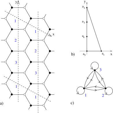
Figure 9: The $\mathbb{C}^{3}/\mathbb{Z}_{3}$ theory: a) dimer configuration b) toric diagram c) quiver diagram.

We can repeat this analysis for the whole family of generalized conifolds of type $A_{k-1}$: they are obtained by modifying the toric theories with geometry the quotient $\mathbb{C}^{3}/\mathbb{Z}_{k}$. The toric diagram $\mathcal{C}$ of $\mathbb{C}^{3}/\mathbb{Z}_{k}$ is:

$$(0,0,1)\quad(1,0,1)\quad(0,k,1)$$ (6.24)

and its dual $\mathcal{C}^{*}$ is generated over the integers by the vectors:

$$(0,1,0)\quad(-k,-1,k)\quad(1,0,0)\quad(-1,0,1)$$ (6.25)

The gauge theory has a dimer made up of $F=k$ gauge groups, $V=2k$ superpotential terms and $E=3k$ chiral fields. The faces are all hexagons aligned in a single column and with the identifications as in Figure 9a). Up to the adjoint fields the quiver is the same as for the generalized conifolds of type $A_{k-1}$: among the $3k$ fields there are $k$ $X_{i}$ and $k$ $\tilde{X}_{i}$, like for the generalized conifolds, and the remaining fields are the adjoints $Y_{ii}$, to which we will have to give mass. We draw in Figure 9 the dimer, toric diagram and quiver in the case $k=3$: modifying this theory we will get again the generalized conifold of type $A_{2}$.

The minimal set of gauge invariants for the theory $\mathbb{C}^{3}/\mathbb{Z}_{k}$ consists of $z$, $w$, $x_{i}$, $i=1,\ldots k$, defined in (6.7) plus the $k$ adjoints $Y_{ii}$. It is easy to see that the $\Psi$-map for the toric theory is

$$\begin{array}[]{l@{\quad}l}w\rightarrow(0,1,0)&z\rightarrow(-k,-1,k)\\ Y_{11},\ldots Y_{kk}\rightarrow(1,0,0)&x_{1},\ldots x_{k}\rightarrow(-1,0,1)\end{array}$$ (6.26)

From this $\Psi$-map it is easy to see that the singularity is defined by the equation: $zw=x_{1}^{k}$ in the four variables: $z$, $w$, $x_{1}$, $Y_{11}$.

The superpotential for the original toric theory is:

$$W_{T^{3}}=\sum_{i=1}^{k}Y_{ii}x_{i}-Y_{ii}x_{i-1}$$ (6.27)

where the index $i$ is periodic with period $k$. The massive terms $Y_{ii}^{2}$ are mesons mapped to $(2,0,0)$, as it is obvious from (6.26), and again the quotient is with respect to $\vec{d}=(2,0,0)-(0,0,1)=(2,0,-1)$. We have to add to the superpotential (6.27) all mesons mapped to points: $(0,0,1)$, $(2,0,0)$, $(-2,0,2)$. We find the superpotential:

$$W_{T^{2}}=\left(\sum_{i=1}^{k}Y_{ii}\right)\left(\sum_{j=1}^{k}x_{j}\right)+\left(\sum_{i=1}^{k}Y_{ii}^{2}\right)+\left(\sum_{i=1}^{k}x_{i}^{2}\right)$$ (6.28)

where again we have understood generic coefficients in front of every term. Integrating out the massive fields $Y_{ii}$ one recovers the superpotential of the generalized conifolds of type $A_{k-1}$ (6.9), again with generic coefficients in front of each term. Therefore we see that the $T^{2}$ theories of generalized conifolds of type $A_{k-1}$ are obtained by quotienting the theories $\mathbb{C}^{3}/\mathbb{Z}_{k}$ with respect to: $\vec{d}=(2,0,-1)$.

We can perform again a change of coordinates using the same matrix $A$ in equation (6.18), that sends $\vec{d}\rightarrow(0,0,1)$. The vectors of $\mathcal{C}^{*}$ in (6.25) are sent respectively to the points:

$$(1,0,0)\quad(k-1,k,-k)\quad(1,1,0)\quad(1,1,-1)$$ (6.29)

and quotienting with respect to $(0,0,1)$ we find that the integer generators of $\mathcal{C}^{*}_{T^{2}}$ are:

$$w\rightarrow(1,0)\quad x_{1},\cdots x_{k}\rightarrow(1,1)\quad z\rightarrow(k-1,k)$$ (6.30)

Note that the points $(1,0)$, $(k-1,k)$ have multiplicities 1, whereas the point $(1,1)$ has multiplicity 2, since, as discussed above, there are $k-2$ independent linear relations between the mesons $x_{1}\ldots x_{k}$, in agreement with the fact that there are 2 points in $\mathcal{C}^{*}$ ($(1,1,0)$ and $(1,1,-1)$) projected to $(1,1)$. Note that when $k=3$ the cone $\mathcal{C}^{*}_{T^{2}}$ is equivalent to that in Figure 8 b).

It is not difficult to resolve the singularity $\mathbb{C}^{3}/\mathbb{Z}_{k}$ and find through equation (5.26) [15] the character $C_{T^{3}}(q)$; after changing coordinates with the matrix $A$ (6.18) we obtain:

$$C_{T^{3}}(q)=\frac{q_{1}q_{3}}{\left(1-q_{1}q_{2}\right)\left(q_{3}-q_{1}q_{2}\right)}\left[\frac{1}{1-q_{1}}+\frac{q_{3}^{k}}{q_{3}^{k}q_{1}-q_{1}^{k}q_{2}^{k}}\right]$$ (6.31)

The character $C_{T^{2}}(q)$ for the generalized conifold of type $A_{k-1}$ is obtained by setting $q_{3}=1$ in the previous formula. Performing the limit (5.30) on $C_{T^{2}}(q)$, or equivalently on (6.31) and then setting $b_{3}=0$, we find the normalized volume for the basis of the generalized conifolds with a Sasaki metric:

$$V_{T^{2}}(b_{1},b_{3})=\frac{k}{b_{1}\left(b_{1}+b_{2}\right)\left(\left(k-1\right)b_{1}+k\,b_{2}\right)}$$ (6.32)

which in the case $k=3$ is equal to that in (6.22) computed through the SPP.

The equations $\Delta=\vec{m}\cdot\vec{b}$ using the generating vectors in (6.30) are:

$$b_{1}=\frac{3}{4}k\quad b_{1}+b_{2}=\frac{3}{2}\quad(k-1)b_{1}+k\,b_{2}=\frac{3}{4}k$$ (6.33)

that allow to find the position of the Reeb vector for a Sasaki-Einstein metric: $(b_{1},b_{2})=(3/4\,k,3/2-3/4\,k)$. Inserting this value into (6.32) we find for the normalized volume of the generalized conifold of type $A_{k-1}$:

$$V_{T^{2}}=\frac{32}{27\,k}$$ (6.34)

which again agrees with the results from a-maximization (6.11), according to the AdS/CFT predictions (5.43). Our formula for the volume (6.34) agrees with the results of reference [49], which describes an alternative method for computing $\textrm{Vol}(H)$ when the CY cone $C(H)$ is defined by a single polynomial equation.

7 Other examples

In this Section we study the toric theories $Y^{2,1}$ and $L^{1,5;2,4}$ and try to modify them adding to their superpotential mesons mapped to: $\vec{m}_{0}+k\vec{d}$ in order to obtain theories with isometry $T^{2}$. In particular our purpose is to see on concrete examples whether it is possible to modify the toric theories keeping the moduli space three-dimensional. Consider for instance the $\mathcal{N}=4$ quiver gauge theory: it has three chiral fields and a superpotential with two terms canceling in the abelianized version of the theory. If we add superpotential terms that are non zero also when the gauge group is $U(1)$ then we are introducing non trivial F-terms and hence the dimension of the moduli space is necessarily less than three. A similar situation happens in the conifold theory $T^{1,1}$: there are $4$ chiral fields, a superpotential equal to zero in the abelian case and one D-term (recall that the number of independent D-terms is equal to the number of gauge groups minus one: the sum of all charges for all gauge groups is zero). Hence the moduli space is three dimensional, but as soon as one introduces superpotential terms and hence non trivial F-terms, the dimension of the moduli space is reduced.

Therefore we choose here to start from the more complicated toric theories $Y^{2,1}$ and $L^{1,5;2,4}$, that have more chiral fields and a non zero superpotential also in the abelian theory. We add superpotential terms as explained in Section 4 with all generic coefficients (we suppose that the coefficients of the toric terms are non zero), and try to see whether there are suitable choices of these coefficients in the superpotential that allow the existence of a three-dimensional moduli space.

To do this we can work using the $E$ chiral fields as complex variables: we write the F-term equations and solve for $E-F-2$ chiral fields (supposing at generic points all the chiral fields different from zero) in function of $F+2$ chiral fields, where $F$ is the number of gauge groups. We have to impose that the remaining F-term equations are satisfied: this gives non trivial constraints on the coefficients in the superpotential. The D-terms (that are independent from the superpotential) will reduce of $F-1$ the dimension of the $F+2$ dimensional manifold, leaving a three-dimensional cone. If the conditions on the coefficients in the superpotential can be satisfied also with non zero coefficients for (some of) the non toric terms, then we have constructed three-dimensional non toric ($T^{2}$) complex cones. An alternative and equivalent way is to work with mesons, we associate a complex variable to each of the mesons that generate loops in the quiver; the moduli space in this case can be expressed as a (typically non complete) intersection in this space of complex variables: since mesons are gauge invariants, we do not have to take into account D-terms and quotients with respect to the corresponding charges. There are non linear algebraic relations among mesons due to their composition in terms of chiral fields, plus linear relations induced by F-terms and depending on the coefficients appearing in the superpotential. Imposing again that the resulting locus is three dimensional we obtain the conditions on coefficients in the superpotential.

Consider now the theory for $Y^{2,1}$; we will not give all the details that can be found in the literature [6]. The toric diagram $\mathcal{C}$ for $Y^{2,1}$ is generated by the vectors:

$$A=(0,0,1)\quad B=(1,0,1)\quad C=(0,2,1)\quad D=(-1,1,1)$$ (7.1)

The generators of the dual cone $\mathcal{C}^{*}$ over integer numbers are the nine vectors:

$$\begin{array}[]{lllll}(0,1,0)&(-2,-1,2)&(1,-1,2)&(1,1,0)&(1,0,1)\\ (-1,0,1)&(-1,-1,2)&(0,-1,2)&(0,0,1)&\end{array}$$ (7.2)

In our analysis we have added to the superpotential mesons mapped to these generators of $\mathcal{C}^{*}$, since they are irreducible mesons (they are not the product of smaller loops) and hence simpler. For some choices of the direction $\vec{d}$ along which to perform the quotient the moduli space is a three dimensional $T^{2}$ cone; we sum up our results:

$$\begin{array}[]{l@{\quad}l@{\quad}c}\,\,\,\,\,\,\,\vec{d}&\textrm{mesons in superpotential}&3d\,\textrm{complex cone}\,T^{2}\\ (1,0,0)&(1,0,1),(0,0,1),(-1,0,1)&\textrm{Yes}\\ (-1,-1,1)&(1,1,0),(0,0,1),(-1,-1,2)&\textrm{Yes}\\ (0,-1,1)&(0,1,0),(0,0,1),(0,-1,2)&\textrm{Yes}\\ (1,-1,1)&(0,0,1),(1,-1,2)&\textrm{No}\\ (-2,-1,1)&(0,0,1),(-2,-1,2)&\textrm{No}\end{array}$$ (7.3)

We have repeated the analysis for $L^{1,5;2,4}$ whose toric diagram $\mathcal{C}$ is:

$$(0,0,1)\quad(1,0,1)\quad(0,2,1)\quad(-2,1,1)$$ (7.4)

The dual cone $\mathcal{C}^{*}$ is generated over integers by the vectors:

$$\begin{array}[]{llll}(0,1,0)&(-2,-1,2)&(1,-2,4)&(1,2,0)\\ (-1,-1,2)&(-1,0,1)&(0,-1,2)&(0,0,1)\\ (1,-1,3)&(1,0,2)&(1,1,1)&\end{array}$$ (7.5)

Again we have added to the superpotentials mesons mapped to these generators of $\mathcal{C}^{*}$. The results are:

$$\begin{array}[]{l@{\quad}l@{\quad}c}\,\,\,\,\,\,\,\vec{d}&\textrm{mesons in superpotential}&3d\,\textrm{complex cone}\,T^{2}\\ (0,-1,1)&(0,1,0),(0,0,1),(0,-1,2)&\textrm{Yes}\\ (-2,-1,1)&(0,0,1),(-2,-1,2)&\textrm{No}\\ (-1,-1,1)&(0,0,1),(-1,-1,2)&\textrm{Yes}\\ (-1,0,0)&(0,0,1),(-1,0,1)&\textrm{Yes}\\ (1,-2,3)&(0,0,1),(1,-2,4)&\textrm{No}\\ (1,-1,2)&(0,0,1),(1,-1,3)&\textrm{Yes}\\ (1,0,1)&(0,0,1),(1,0,2)&\textrm{Yes}\\ (1,1,0)&(0,0,1),(1,1,1)&\textrm{Yes}\\ (1,2,-1)&(0,0,1),(1,2,0)&\textrm{Yes}\\ \end{array}$$ (7.6)

We see therefore that the existence of 3d complex cones (with isometry group $T^{2}$) obtained by modifying toric theories is quite a common feature. Indeed all the vectors $\vec{d}$ considered here along which we performed the quotient satisfy the condition (4.8) for having finite multiplicities (note that the proof of the equivalence of a-maximization and volume minimization in the next Section relies only on this property); yet for some of them there is no three dimensional complex cone with reduced isometry $T^{2}$. It would be interesting to understand whether there are conditions on $\vec{d}$ corresponding to the request of a three dimensional non toric moduli space.

As a final remark we point out that it is not always obvious that the deformation we add to the toric theory is relevant: in some cases presented in this Section the new superpotential terms have dimension greater than $3$ computed at conformal points of the original toric theory. However recall that we are changing all the coefficients in the superpotential (and possibly the gauge couplings) so that some operator may become (marginally) relevant. We have checked on these examples that the central charge $a$ of the deformed theories is always less than in the original toric theories.

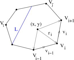
Figure 10: The toric diagram $P$ where volume minimization for the $T^{3}$ theory must be performed. For $T^{2}$ theories volume minimization is performed on a line segment $L$ inside $P$.

8 a-maximization and volume minimization

In this Section we prove that the results of a-maximization and volume minimization match the predictions of AdS/CFT (5.43) in the general class of theories obtained by modifying toric theories as explained in Section 4. We make a proposal to identify the space where volume minimization [15] should be performed when the isometry is $T^{2}$ (in the case $T^{1}$ this locus is reduced to a single point).

Let us start from a toric AdS/CFT correspondence: in our conventions the vertices of the toric diagram are the points: $V_{i}=(x_{i},y_{i},1)$ that generate the fan $\mathcal{C}$. As in Section 3 we also introduce the sides of the toric diagram: $v_{i}\equiv(x_{i+1},y_{i+1})-(x_{i},y_{i})$ and the vectors joining the trial Reeb $(x,y)$ with the vertices: $r_{i}\equiv(x_{i},y_{i})-(x,y)$, see Figure 10. The Reeb vector for a Sasaki-Einstein metric $\vec{b}=3(\bar{x},\bar{y},1)$ is the minimum of the volume function for a Sasaki metric $V(\vec{b})$ when $\vec{b}$ lies on the plane $z=3$: $\vec{b}=3(x,y,1)$, and the trial point $(x,y)$ lies inside the toric diagram $P$ [14] (the expression for the volume of $H$ in function of $(x,y)$ is reported also in equation (3.7)). The proof of the equivalence of volume minimization and a-maximization [20] lies on the fact that if we parametrize the charges $a_{i}$ as (3.3):

$$a_{i}\rightarrow a_{i}(x,y)\equiv\frac{2l_{i}}{\displaystyle\sum_{j=1}^{d}l_{j}}\qquad\textrm{with}\qquad l_{i}\equiv\frac{\langle v_{i-1},v_{i}\rangle}{\langle r_{i-1},v_{i-1}\rangle\langle r_{i},v_{i}\rangle}$$ (8.1)

then the matching (5.43) is true for every $(x,y)$ inside the toric diagram $P$ [20]:

$$a(x,y)=\frac{1}{4V(x,y)}\qquad\textrm{with}\qquad a(x,y)\equiv a(a_{1}(x,y),\ldots a_{d}(x,y))$$ (8.2)

where $V(x,y)$ is the normalized volume function $V(\vec{b})$ for a Sasaki metric computed at the trial Reeb vector: $\vec{b}=3(x,y,1)$. Note that parametrization (8.1) automatically satisfies condition (4.2). Moreover the derivatives of the trial charge $a(a_{1},\ldots a_{d})$ are zero along the $d-3$ baryonic symmetries (4.4) and on the surface $a_{i}=a_{i}(x,y)$ parametrized by $(x,y)$ [20]:

$$\sum_{i=1}^{d}B_{i}\left(\frac{\partial a}{\partial a_{i}}\right)_{|a_{i}\rightarrow a_{i}(x,y)}=0\qquad B_{i}\,\,\textrm{any baryonic symmetry:}\,\,\sum_{i=1}^{d}B_{i}\vec{V}_{i}=0$$ (8.3)

Therefore also a-maximization in the $d-1$ independent parameters $a_{i}$ is reduced to an extremization problem in the variables $(x,y)$.

Moreover, as proved in [14, 20], see also Section 3, for every $(x,y)$ inside the toric diagram $P$ we have the following relations:

$$\sum_{i=1}^{d}a_{i}(x,y)\vec{V}_{i}=2(x,y,1)\quad\Rightarrow\quad\frac{3}{2}\sum_{i=1}^{d}\left(\vec{m}\cdot\vec{V}_{i}\right)a_{i}(x,y)=3(x,y,1)\cdot\vec{m}$$ (8.4)

where the second equality is an extension of $\Delta=\vec{b}\cdot\vec{m}$ to the whole interior of the polygon $P$. $\vec{m}$ is a point in $\mathcal{C}^{*}$ and as usual represents the charges of a meson under $\Psi$-map.

Let us now modify the original toric $T^{3}$ theory to a $T^{2}$ theory by adding superpotential terms of the form $\vec{m}_{0}+k\vec{d}$, as in Section 4; we will suppose that this gauge theory (for some suitable choice of coefficients in the superpotential) admits a three-dimensional moduli space of vacua and that multiplicities of holomorphic functions over this three-dimensional cone are counted as explained in Section 4. The first step is to try to understand a-maximization: the trial $a$ charge is the same function $a(a_{1},\ldots a_{d})$ of the toric case but we have to add the new constraint (4.5) besides the usual condition (4.2). Consider the plane $Q$ perpendicular to the vector $\vec{d}$ and passing through the origin. The plane containing the toric diagram $P$ is perpendicular to $\vec{m}_{0}\equiv(0,0,1)$: it is the plane $z=1$ in our conventions. These two planes in $\mathbb{R}^{3}$ intersect on a line since $\vec{d}$ cannot be proportional to $\vec{m}_{0}\in\mathcal{C}^{*}$ because of condition (4.8) and in particular the plane $Q$ intersects the polygon $P$ on a line segment $L$ interior to $P$, look at Figure 10; in fact condition (4.8) is equivalent to the request that there exist $\bar{i}$, $\bar{j}$ such that $\vec{d}\cdot\vec{V}_{\bar{i}}>0$ and $\vec{d}\cdot\vec{V}_{\bar{j}}<0$. The points $(x,y)\in L$ are characterized by: $\vec{d}\cdot(x,y,1)=0$.

Interestingly if we restrict $(x,y)$ to vary along the line $L$ and use the same parametrization (8.1) and equation (8.4) we find that the new request (4.5) in the case $T^{2}$ is satisfied:

$$\sum_{i=1}^{d}\left(\vec{d}\cdot\vec{V}_{i}\right)a_{i}(x,y)=0\qquad\quad\forall(x,y)\in L$$ (8.5)

a-maximization must be performed on $d-2$ independent variables $a_{i}$; but note that since $L\subset P$ and since, as observed in Section 4, the $d-3$ baryonic symmetries $B_{i}$ are the same for the $T^{3}$ and the $T^{2}$ (or $T^{1}$) theories then equation (8.3) tells us that along $L$ we have decoupled baryonic symmetries also for the $T^{2}$ theory. a-maximization is reduced to an extremization problem in one variable, as expected since there is now only one flavor symmetry. We have to maximize the same function $a(x,y)$ of the toric case but along $L$ and not on the whole interior of $P$. Note therefore that $a_{T^{2}}\leq a_{T^{3}}$ and recall that in our theories (that have $\textrm{tr}R=0$ and hopefully a supergravity dual) the central charges $a$ and $c$ are equal. This is in agreement with the decreasing of $a=c$ along the renormalization group flow: we have added relevant terms to the $T^{3}$ theory and then flown to new superconformal IR fixed points, corresponding to $T^{2}$ theories.

Let us consider now meson charges; after the introduction of the superpotential terms that break one flavor symmetries, aligned vectors $\vec{m}+k\vec{d}$ in the toric $\mathcal{C}^{*}$ are identified: we have to project perpendicularly each integer point $\vec{m}\in\mathcal{C}^{*}$ on the plane $Q$ to find the new cone of charges for the theory $T^{2}$. The scaling dimensions of mesons in the $T^{2}$ theory can be computed as usual with the $\Psi$-map: $\Delta=3/2\sum_{i}(\vec{m}\cdot\vec{V}_{i})a_{i}(\bar{x},\bar{y})$ and we know from the previous analysis that $(\bar{x},\bar{y})$ lie on $L$. The formula for the scaling dimensions of mesons can be extended to the equality, which holds for all $(x,y)\in L$:

$$\frac{3}{2}\sum_{i=1}^{d}\left(\vec{m}\cdot\vec{V}_{i}\right)a_{i}(x,y)=3(x,y,1)\cdot\vec{m}\qquad\vec{m}\sim\vec{m}+k\vec{d},\quad(x,y)\in L$$ (8.6)

which is the same as (8.4), but we underline that both sides of the equality are invariant under $\vec{m}\sim\vec{m}+k\vec{d}$ if $(x,y)\in L$, again because of (8.4). All of this tells us that the cone of charges for holomorphic functions of the $T^{2}$ theory is obtained by projecting perpendicularly each integer point $\vec{m}$ in the toric $\mathcal{C}^{*}$ on the plane $Q$; we will call $\pi$ the orthogonal projection over $Q$ (4.7). The Reeb vector $\vec{b}$ lies now on $Q$ and the scalar product in $\Delta=\vec{b}\cdot\vec{m}$ is the restriction of the scalar product of the toric theory to the plane $Q$. In our examples we computed the Reeb vector from a-maximization imposing that for all mesons $\Delta=\vec{b}\cdot\vec{m}$ and it is evident from this discussion that these equations are always consistent since they admit the solution $\vec{b}=3(\bar{x},\bar{y},1)$, with $(\bar{x},\bar{y})\in L$ coming from a-maximization $a(x,y)$ along $L$.

Let us now try to understand the volume function $V_{T^{2}}(\vec{b})$ for a Sasaki metric on the base of the cone, where $\vec{b}$ varies inside $Q$. Suppose to perform an $SL(3,\mathbb{Z})$ that sends $\vec{d}$ in, say, $(1,0,0)$; this is always possible since $\vec{d}$ is a primitive integer vector. In this frame the plane $Q$ is the plane $(y,z)$. Under the hypothesis that multiplicities of holomorphic functions are computed, as explained in Section 4, by counting the number of integer points of $\mathcal{C}^{*}$ projected to the same point on the plane $Q$, then the character $C_{T^{2}}(q_{2},q_{3})$ is equal to $C_{T^{3}}(1,q_{2},q_{3})$. And from equation (5.30) it follows easily:

$$V_{T^{2}}(b_{2},b_{3})=\lim_{t\rightarrow 0}t^{3}C_{T^{2}}(e^{-tb_{2}},e^{-tb_{3}})=\lim_{t\rightarrow 0}t^{3}C_{T^{3}}(1,e^{-tb_{2}},e^{-tb_{3}})=V_{T^{3}}(0,b_{2},b_{3})$$ (8.7)

More generally we see that the function $V_{T^{2}}$ is simply the volume function of the toric case $V_{T^{3}}$ restricted to the plane $Q$ .

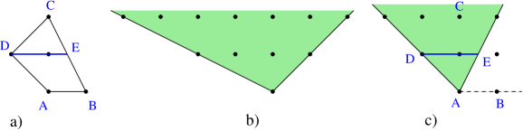
Figure 11: a) Toric diagram for $Y^{21}$ with the line $L\equiv D\,E$ corresponding to the quotient $\vec{d}=(0,-1,1)$. b) The cone $\mathcal{C}^{*}_{T^{2}}$ of charges for holomorphic functions. c) The direct cone $\mathcal{C}_{T^{2}}$ in green, dual of $\mathcal{C}^{*}_{T^{2}}$, where the function $V_{T^{2}}$ is defined.

It is clear at this point that the matching $a_{T^{2}}=1/(4V_{T^{2}})$ always holds with $V_{T^{2}}$ equal to the volume function computed at the Reeb vector $\vec{b}$ coming from a-maximization; more generally, as a simple restriction of (8.2), the two trial functions $a_{T^{2}}(x,y)$ and $V_{T^{2}}(x,y)$ agree on the whole line segment $L$:

$$a_{T^{2}}(x,y)=\frac{1}{4V_{T^{2}}(x,y)}\qquad(x,y)\in L$$ (8.8)

It is natural at this point to identify the line $L$ as the locus where to perform volume minimization [15]. We suggest that this is the case for the class of non toric theories introduced in Section 4.

As an example consider the toric theory $Y^{21}$ with $\mathcal{C}$ and $\mathcal{C}^{*}$ generated by vectors in (7.1) and (7.2) respectively, and consider the $T^{2}$ quotient with vector $\vec{d}=(0,-1,1)$, that admits a three dimensional cone as a moduli space of vacua, as told in Section 7. Line $L$ is the intersection of the plane $Q$ perpendicular to $\vec{d}$: $-y+z=0$, with the plane of the toric diagram: $z=1$, and hence is the line segment with $z=1$, $y=1$ with extremal points $D=(-1,1,1)$ and $E=(1/2,1,1)$; it is drawn in Figure 11a). We can apply the $SL(3,\mathbb{Z})$ transformation $S=((1,0,0),(0,1,1),(0,0,1))$ to the points of $\mathcal{C}^{*}$; the vector $\vec{d}$ is mapped to $(0,0,1)$. The first four generating vectors in (7.2) that generate $\mathcal{C}^{*}$ over real numbers are mapped by $S$ into:

$$(0,1,0)\quad(-2,1,2)\quad(1,1,2)\quad(1,1,0)$$ (8.9)

With these coordinates the cone $\mathcal{C}^{*}_{T^{2}}=\pi(\mathcal{C}^{*})$ is obtained by projecting these vectors on the plane $Q=(x,y)$ ($\pi$ stands for the orthogonal projection on the plane $Q$). Hence $\mathcal{C}^{*}_{T^{2}}$ is generated over real numbers by $(-2,1)$ and $(1,1)$ and it is drawn in Figure 11b). Transforming the points in (7.1) with ${}^{t}S^{-1}$ we get:

$$A=(0,0,1)\quad B=(1,0,1)\quad C=(0,2,-1)\quad D=(-1,1,0)$$ (8.10)

and the point $E$ in the new coordinates is $E=(1/2,1,0)$. In Figure 11 we show the projection of $\pi(\mathcal{C})$ on the plane $Q$; it is generated by $(1,0)$, $(-1,1)$ over real numbers. In the same Figure we also draw in green the cone over $L$, that in the intersection $\mathcal{C}\cap Q$, generated by vectors $(1,2)$, $(-1,1)$: on the interior of this two dimensional cone the function $V_{T^{2}}$ is positive and well defined, and it is convex on the segment $L=D\,E$ where volume minimization has to be performed. Interestingly we note that the cone $\mathcal{C}\cap Q$ is just the dual of $\mathcal{C}^{*}_{T^{2}}$, and hence we will call it $\mathcal{C}_{T^{2}}$:

$$\mathcal{C}_{T^{2}}\equiv\left(\mathcal{C}^{*}_{T^{2}}\right)^{*}\equiv\left(\pi(\mathcal{C}^{*})\right)^{*}=\mathcal{C}\cap Q$$ (8.11)

To see (8.11) suppose that $\vec{n}\in\mathcal{C}\cap Q$, then $\vec{n}\cdot\vec{m}\geq 0$, for any $\vec{m}\in\mathcal{C}^{*}$. But since $\vec{n}$ belongs to $Q$, then $\vec{n}\cdot\vec{m}=\vec{n}\cdot(\vec{m}+k\vec{d})\geq 0$ and we can choose $k$ to obtain: $\vec{n}\cdot\pi(\vec{m})\geq 0$, hence we have shown that: $\mathcal{C}\cap Q\subseteq\mathcal{C}_{T^{2}}$. Conversely if $\vec{n}$ is in $\mathcal{C}_{T^{2}}$ then it is a vector in $Q$ such that $\vec{n}\cdot\pi(\vec{m})\geq 0$ for any $\vec{m}\in\mathcal{C}^{*}$. But again for vectors $\vec{n}\in Q$ we have: $\vec{n}\cdot\vec{m}=\vec{n}\cdot\pi(\vec{m})\geq 0$ for any $\vec{m}\in\mathcal{C}^{*}$, therefore $\vec{n}$ also belongs to $\mathcal{C}$. Hence also $\mathcal{C}_{T^{2}}\subseteq\mathcal{C}\cap Q$ holds.

We can repeat the same analysis for $T^{1}$ theories: there are now two independent vectors $\vec{d}_{1}$, $\vec{d}_{2}$, and two further constraints to be imposed on trial charges $a_{i}$ (4.6). Let $Q_{1}$ and $Q_{2}$ be the planes perpendicular to $\vec{d}_{1}$ and $\vec{d}_{2}$ respectively, and $L_{1}$ and $L_{2}$ their intersection with the toric diagram $P$ on the plane $z=1$. Then the two constraints (4.6) are satisfied by $a_{i}(x,y)$ in (8.1) on the point $N$ defined as the intersection of the line segments $L_{1}$ and $L_{2}$. Note that $N$ lies in the interior of the convex polygon $P$; in fact the point $N$ is the intersection of the plane $z=1$ with the line $R$ passing through the origin and perpendicular to the plane generated by $\vec{d}_{1}$, $\vec{d}_{2}$. This line $R$ belongs to the direct cone $\mathcal{C}\cup(-\mathcal{C})$ as explained in Section 4. a-maximization must be performed on a space of $d-3$ independent $a_{i}$, and at point $N$ there are just $d-3$ baryonic directions with zero derivatives for the trial $a$ function. The Reeb vector is determined in terms of the coordinates of $N$ as: $\vec{b}=3(x_{N},y_{N},1)$ and lies on $R$. The cone for mesonic charges can be obtained as the projection of the toric $\mathcal{C}^{*}$ on the line $R$; we will call $\Pi$ the orthogonal projection over the line $R$ (4.9). Equality (8.6) is still true and non ambiguous under $\vec{m}\sim\vec{m}+k\vec{d}_{1}+h\vec{d}_{2}$ if $(x,y)$ coincides with $N$. The volume function $V_{T^{1}}(\vec{b})$ is a restriction of $V_{T^{3}}(\vec{b})$ to the line $R$. There is no volume minimization to perform; the central charge $a$ and the volume of a Sasaki-Einstein metric agree (5.43) again as a simple restriction of the identity (8.2) to the point $N$.

Acknowledgments

We would like to thank Sergio Benvenuti, Amihay Hanany, Christopher P. Herzog, Dario Martelli, David Vegh and in particular Alessandro Tomasiello for invaluable discussions. D.F. is grateful to Elena Andreini, Giulio Bonelli, Barbara Fantechi, Luca Martucci for very useful and patient discussions, to Angel M.Uranga for helpful correspondence and to Andrea Brini, Diego Gallego and Houman Safaai for constant support. We thank MIT for kind hospitality while part of this work was done. This work is supported in part by INFN (and Bruno Rossi exchange program) and MURST under contract 2005-024045-004 and 2005-023102 and by the European Community’s Human Potential Program MRTN-CT-2004-005104.

Appendix A Review of toric geometry and quiver gauge theory

The correspondence between quiver gauge theories (considering equivalent two theories that flow to the same IR fixed point) and singularities is complete in the toric case [16, 17, 18]; we will introduce now the elements of this correspondence that will be used in the following. Roughly speaking a six dimensional manifold is toric if it has at least $U(1)^{3}$ isometry. All geometrical information about toric CY cones are encoded in the fan $\mathcal{C}$ [22], in this case a cone in $\mathbb{Z}^{3}$ defined by $d$ vectors $V_{i}$. The Calabi-Yau condition requires that all vectors $V_{i}$ lie on a plane. In our conventions the vectors $V_{i}$ will lie on the plane with third coordinate $z=1$. By ignoring the third coordinate, we can consider the toric diagram, a convex polygon in the plane with integer vertices, which is just the intersection of the fan with the plane $z=1$. The (p,q) web is the set of vectors perpendicular to the edges of the toric diagram and with the same length as the corresponding edges. In the toric case the gauge theory is completely identified by the periodic quiver, a diagram drawn on $T^{2}$ (it is the “lift” of the usual quiver to the torus): nodes represent $SU(N)$ gauge groups, oriented links represent chiral bifundamental multiplets and faces represent the superpotential: the trace of the product of chiral fields of a face gives a superpotential term. Equivalently the gauge theory is described by the dimer configuration, or brane tiling, the dual graph of the periodic quiver, drawn also on a torus $T^{2}$. In the dimer the role of faces and vertices is exchanged: faces are gauge groups and vertices are superpotential terms. The dimer is a bipartite graph: it has an equal number of white and black vertices (superpotential terms with sign + or - respectively) and links connect only vertices of different colors.

By applying Seiberg dualities to a quiver gauge theory we can obtain different quivers that flow in the IR to the same CFT: to a toric diagram we can associate different quivers/dimers describing the same physics. It turns out that in the toric case one can always find phases where all the gauge groups have the same number of colors; these are called toric phases. Seiberg dualities keep constant the number of gauge groups $F$, but may change the number of fields $E$, and therefore the number of superpotential terms $V=E-F$ (since the dimer is on a torus we have: $V-E+F=0$.). A zig-zag path in the dimer is a path of links that turn maximally left at a node, maximally right at the next node, then again maximally left and so on [17]. It was noted that every link of the dimer belongs to exactly two different zig-zag paths, oriented in opposite directions. Moreover for dimers representing consistent theories the zig-zag paths are closed non-intersecting loops. There is a one to one correspondence between zig-zag paths and legs of the $(p,q)$ web: the homotopy class in the fundamental group of the torus of every zig-zag path is given by the integer numbers $(p,q)$ of the corresponding leg in the $(p,q)$ web and this fact was used in [17] to find a general algorithm to reconstruct the gauge theory from the geometry in the toric case.

Non anomalous $U(1)$ symmetries play a very important role in the gauge theory. Here we review how to count and parametrize them and how to compute the charge of a certain link in the dimer. For smooth horizons $H$ we expect $d-1$ global non anomalous symmetries, where $d$ is the number of sides of the toric diagram in the dual theory. We can count these symmetries from the number of massless vectors in the $AdS$ dual. Since the manifold is toric, the metric has three $U(1)$ isometries. One of these (generated by the Reeb vector) corresponds to the R-symmetry while the other two give two global flavor symmetries in the gauge theory. Other gauge fields in $AdS$ come from the reduction of the RR four form on the non-trivial three-cycles in the horizon manifold $H$, and there are $d-3$ three-cycles in homology [9] when $H$ is smooth. On the field theory side, these gauge fields correspond to baryonic symmetries. Summarizing, the global non anomalous symmetries are:

$$U(1)^{d-1}=U(1)^{2}_{F}\times U(1)^{d-3}_{B}$$ (A.1)

If the horizon $H$ is not smooth (that is the toric diagram has integer points lying on the edges), equation (A.1) is still true with $d$ equal to the perimeter of the toric diagram in the sense of toric geometry (d = number of vertices of toric diagram + number of integer points along edges). In this paper we use the fact that these $d-1$ global non anomalous charges can be parametrized by $d$ parameters $a_{1},a_{2},\ldots,a_{d}$ [20], each associated with a vertex of the toric diagram or a point along an edge, satisfying the constraint:

$$\sum_{i=1}^{d}a_{i}=0$$ (A.2)

The $d-3$ baryonic charges are those satisfying the further constraints [9]:

$$\sum_{i=1}^{d}a_{i}V_{i}=0$$ (A.3)

where $V_{i}$ are the vectors of the fan: $V_{i}=(x_{i},y_{i},1)$ with $(x_{i},y_{i})$ the coordinates of integer points along the perimeter of the toric diagram. The R-symmetries are parametrized with the $a_{i}$ in a similar way of the other non-baryonic global symmetry, but they will satisfy the different constraint

$$\sum_{i=1}^{d}a_{i}=2$$ (A.4)

due to the fact that the terms in the superpotential must have $R$-charges equal to two.

The simplest algorithm to compute the charge of a generic link in the dimer in function of the parameters $a_{i}$ is probably the one that make use of the zig-zag paths. Consider the two zig-zag paths to which a link in the dimer belongs. They correspond to two vectors $v_{i}=(p_{i},q_{i})$ and $v_{j}=(p_{j},q_{j})$ in the $(p,q)$ web. Then the charge of the link is given by the sum of the parameters $a_{i+1}+a_{i+2}\ldots+a_{j}$ between the vectors $v_{i}$ and $v_{j}$ as shown in Figure 12. This rule explains the formula for the multiplicities of fields with a given charge [20]: since every link in the dimer corresponds to the intersection of two zig-zag paths, the number of fields with charge $a_{i+1}+a_{i+2}\ldots+a_{j}$ is equal to the number of intersections between the zig zag paths corresponding to $v_{i}$ and $v_{j}$, which is just $\mathrm{det}(v_{i},v_{j})$.

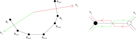
Figure 12: (i) On the left: part of a toric diagram $P$ with the charge distribution (a trial charge $a_{i}$ for every vertex $V_{i}$ ) and two vectors $v_{i}$ and $v_{j}$ of the $(p,q)$-web. (ii) On the right: the corresponding zig-zag paths and the link with charge $a_{i+1}+a_{i+2}+a_{i+3}+a_{i+4}+a_{j}$ according to the recipe explained in the main text.

One can show that this parametrization automatically solve the conditions of vanishing of gauge and superpotential beta functions [20, 21]. The $d-1$ independent free quantities $a_{i}$ parametrize the $d-1$ global abelian symmetry of the gauge theory that can mix with the R-symmetry. The value of $a_{i}$ at the fixed point can be found by using a-maximization.

Appendix B The moduli spaces for $(P)dP_{4}$ theories

We give here more details about the moduli spaces of the $(P)dP_{4}$ theories considered in Section 5. As usual for toric theories, the moduli space of the $T^{3}$ $PdP_{4}$ is determined by the linear relations among the generating vectors of the cone $\mathcal{C}^{*}$. We associate with every generator of $\mathcal{C}^{*}$ in (5.5) a complex coordinate $z_{1}$, $z_{2}$, $z_{3}$, $z_{4}$, $z_{5}$ and $t$ and choose a representative meson among those (F-term equivalent) mapped to the point of $\mathcal{C}^{*}$:

$$\begin{array}[]{c}n_{4}\rightarrow(0,-1,2)\rightarrow z_{4}\quad q_{1}\rightarrow(-1,-1,3)\rightarrow z_{3}\quad n_{8}\rightarrow(0,1,0)\rightarrow z_{1}\\ m_{6}\rightarrow(0,0,1)\rightarrow t\quad n_{1}\rightarrow(-1,0,2)\rightarrow z_{2}\\ n_{5}\rightarrow(1,0,0)\rightarrow z_{5}\end{array}$$ (B.1)

where for the complex coordinates we have used the same notation as in [36]. The equations defining the toric manifold are therefore the five quadrics in $\mathbb{C}^{6}$:

$$z_{1}z_{3}=z_{2}t\quad z_{2}z_{4}=z_{3}t\quad z_{3}z_{5}=z_{4}t\quad z_{2}z_{5}=t^{2}\quad z_{1}z_{4}=t^{2}$$ (B.2)

This is a non complete intersection and it is easy to verify that the moduli space is three-dimensional.

The moduli spaces in the cases of the theories $T^{2}$ and $T^{1}$ are more complicated; interestingly they are still defined as a non complete intersection of five quadrics in $\mathbb{C}^{6}$, with equations generalizing those in (B.2); see also [27] for the $T^{1}$ theory describing $dP_{4}$. In the non toric case $T^{2}$ there may be also a deformation of the complex structure that leaves the manifold a cone. We will deal in this Appendix with the easier case of the $T^{2}$ $PdP_{4}$, with the general superpotential:

$$W_{T^{2}}=a\,(m_{1}+m_{3}+m_{5}+m_{7})-b\,(m_{2}+m_{4}+m_{6}+m_{8})+c\,n_{1}-d\,n_{3}+e\,n_{5}-f\,n_{7}+g\,p_{1}$$ (B.3)

where it is clear that we can rescale the coefficients of the toric terms in this way (if they are non zero). It is easy to see that there are suitable choices of the coefficients in (B.3) allowing a three dimensional moduli space: there are 15 fields and 7 gauge groups, hence 6 independent D-terms (D-terms equations and quotients are independent from the parameters in the superpotential). Therefore if we want a three dimensional manifold, F-terms should reduce the dimension of the manifold of 6: we solve some of the F-term equations with respect to 6 fields (supposing at generic points all chiral fields different from zero); if we impose that the remaining F-term equations are satisfied with these substitutions, we get some complicated conditions on the coefficients in (B.3). It is not difficult to see that these conditions are satisfied with the choice:

$$e=\frac{b^{2}f}{a^{2}-d\,f}\quad g=\frac{a\,b^{4}-a^{5}+2a^{3}d\,f-a\,d^{2}f^{2}}{b^{3}f}\quad c=\frac{a^{4}-b^{4}-a^{2}d\,f}{b^{2}f}$$ (B.4)

Note that there are other branches of solutions that assure a three-dimensional complex moduli space; in the following we will refer to (B.4). The same conditions could have been obtained using directly gauge invariant mesons.

To write the moduli space using only algebraic equations we have to consider the relations among mesons. There are non linear relations following directly from the definitions (5.3) in terms of elementary fields of the 24 generating mesons; hence these relations do not depend on the superpotential but only on the quiver. In our example these non linear relations define a complex 9 dimensional submanifold of $\mathbb{C}^{24}$. A peculiar role is played by the first 20 mesons in (5.3), that is those mapped to generating vectors of the toric $\mathcal{C}^{*}$; the quadratic relations among them are:

$$\begin{array}[]{lllll}m_{1}m_{4}=n_{7}p_{1}&m_{1}m_{5}=n_{4}n_{6}&m_{1}m_{7}=n_{3}n_{7}&m_{1}n_{1}=m_{8}p_{1}&m_{1}n_{2}=n_{7}q_{1}\\ n_{4}p_{1}=m_{1}q_{2}&m_{2}m_{3}=n_{8}p_{2}&m_{2}m_{6}=n_{3}n_{5}&m_{2}m_{8}=n_{4}n_{8}&m_{2}n_{1}=n_{8}q_{2}\\ m_{2}n_{2}=m_{7}p_{2}&n_{3}p_{2}=m_{2}q_{1}&m_{3}m_{5}=n_{1}n_{5}&m_{3}m_{7}=n_{2}n_{8}&m_{3}n_{3}=n_{8}q_{1}\\ m_{3}n_{4}=m_{8}p_{2}&n_{1}p_{2}=m_{3}q_{2}&m_{4}m_{6}=n_{2}n_{6}&m_{4}m_{8}=n_{1}n_{7}&m_{4}n_{3}=m_{7}p_{1}\\ m_{4}n_{4}=n_{7}q_{2}&n_{2}p_{1}=m_{4}q_{1}&m_{5}p_{1}=n_{6}q_{2}&m_{5}p_{2}=n_{5}q_{2}&m_{5}q_{1}=m_{6}q_{2}\\ m_{6}p_{1}=n_{6}q_{1}&m_{6}p_{2}=n_{5}q_{1}&n_{2}n_{3}=m_{7}q_{1}&n_{1}n_{4}=m_{8}q_{2}&n_{5}p_{1}=n_{6}p_{2}\end{array}$$ (B.5)

There are no cubic independent relations and a single independent quartic equation among the first 20 mesons in (5.3): $m_{5}m_{6}n_{7}n_{8}=m_{7}m_{8}n_{5}n_{6}$.

Then we have to intersect this 9 dimensional manifold with the linear space following from F-term relations (LABEL:lineart21), (5.21) and (5.22). Moreover it is easy to see that, once F-term relations are taken into account, the mesons $t_{1}$, $t_{2}$, $t_{3}$ and $t_{4}$ are equal to quadratic polynomials in the first 20 mesons in (5.3), and therefore they can be eliminated. In fact it is easy to check that also all non linear relations involving the $t_{i}$ do not add other independent equations to those we will write. Let us consider therefore the first 20 mesons in (5.3): we can solve the linear constraints (LABEL:lineart21), (5.21) and (5.22) expressing mesons in function of the 6 mesons: $n_{4}$, $q_{1}$, $n_{8}$, $m_{6}$, $n_{1}$, $n_{5}$. Substituting these linear relations in (B.5), using conditions (B.4), we see that there remain only 5 linearly independent quadratic equations:

$$\left(a^{2}-d\,f\right)\,\left(-\left(b^{4}\,t\,z_{2}\right)+a^{2}\,\left(a^{2}-d\,f\right)\,t\,z_{2}+b^{3}\,f\,\left(t^{2}-z_{1}\,z_{4}\right)\right)-b^{4}\,f^{2}\,t\,z_{5}=0$$

$$\left(\left(a^{2}-d\,f\right)\,\left(b^{3}\,f\,t^{2}+a^{2}\,\left(a^{2}-d\,f\right)\,t\,z_{2}-a\,b\,\left(a^{2}-d\,f\right)\,z_{1}\,z_{3}\right)\right)-b^{4}\,f^{2}\,t\,z_{5}=0$$

$$\left(b^{2}\,{\left(a^{2}-d\,f\right)}^{2}\,t^{2}\right)-\left(a^{2}-d\,f\right)\,\left(2\,b^{3}\,f\,t+a^{2}\,\left(a^{2}-d\,f\right)\,z_{2}\right)\,z_{5}+b^{4}\,f^{2}\,{z_{5}}^{2}=0$$

$$a\,b^{5}\,d^{2}\,f^{2}\,z_{2}\,z_{3}-a^{9}\,\left(f\,t+b\,z_{2}\right)\,z_{3}+3\,a^{7}\,d\,f\,\left(f\,t+b\,z_{2}\right)\,z_{3}$$

$$+a^{5}\,\left(b^{5}\,z_{2}-3\,d^{2}\,f^{2}\,\left(f\,t+b\,z_{2}\right)\right)\,z_{3}+a^{3}\,d\,f\,\left(-2\,b^{5}\,z_{2}+d^{2}\,f^{2}\,\left(f\,t+b\,z_{2}\right)\right)\,z_{3}$$

$$+a^{6}\,b^{2}\,f\,\left(f\,t+b\,z_{2}\right)\,z_{4}-2\,a^{4}\,b^{2}\,d\,f^{2}\,\left(f\,t+b\,z_{2}\right)\,z_{4}$$

$$+a^{2}\,b^{2}\,f^{2}\,\left(b^{4}\,t+d^{2}\,f^{2}\,t+b\,d^{2}\,f\,z_{2}\right)\,z_{4}-b^{6}\,f^{3}\,z_{4}\,\left(d\,t+b\,z_{5}\right)=0$$

$$\left(\left(a^{2}-d\,f\right)\,t\,\left(-\left(a^{4}\,z_{3}\right)+b^{4}\,z_{3}+a^{2}\,d\,f\,z_{3}+a\,b^{2}\,f\,z_{4}\right)\right)-b^{5}\,f\,z_{3}\,z_{5}=0$$ (B.6)

where we have relabeled the mesons $n_{4}$, $q_{1}$, $n_{8}$, $m_{6}$, $n_{1}$, $n_{5}$ respectively with the complex variables: $z_{4}$, $z_{3}$, $z_{1}$, $t$, $z_{2}$, $z_{5}$, as in the toric case (B.1). Once linear relations among mesons are kept into consideration, the quartic relation $m_{5}m_{6}n_{7}n_{8}=m_{7}m_{8}n_{5}n_{6}$ can be deduced from equations (B.6). We see therefore that the moduli space of the $T^{2}$ theory is a non complete intersection in $\mathbb{C}^{6}$ of these 5 quadrics; it is easy to verify that the dimension of the complex cone is three.

Indeed not all the parameters appearing in the equations (B.6) are associated with independent complex deformations: to count how many complex deformations of the non toric $T^{2}$ cone are admitted (that leave the manifold a cone) we have to consider how many parameters among the $(a,b,d,f)$ can be reabsorbed through generic linear redefinitions of the complex variables $z_{1},\ldots z_{5},\,t$. It is easy to see that through suitable rescalings of the $z_{1},\ldots z_{5},\,t$ only three parameters can be reabsorbed . We also explicitly checked that the remaining parameter cannot be reabsorbed through generic linear redefinitions of the complex variables. Hence the non toric $T^{2}$ cone (with the choice of relations in (B.4)) admits one complex parameter of deformations.

The case of the $(P)dP_{4}$ theory with isometry $T^{1}$ is analogous to the case $T^{2}$ studied in this Appendix, even though the computations are much more longer. We checked that for suitable values of the coefficients in the superpotential (5.12) the moduli space can still be expressed as a non complete intersection of 5 quadrics in $\mathbb{C}^{6}$. As explained in subsection 5.2, typically we expect no complex deformation for the $T^{1}$ cone that leaves it a cone.

References

- [1] I. R. Klebanov and E. Witten, “Superconformal field theory on threebranes at a Calabi-Yau singularity,” Nucl. Phys. B 536, 199 (1998) [arXiv:hep-th/9807080].
- [2] B. S. Acharya, J. M. Figueroa-O’Farrill, C. M. Hull and B. Spence, “Branes at conical singularities and holography,” Adv. Theor. Math. Phys. 2, 1249 (1999) [arXiv:hep-th/9808014]; D. R. Morrison and M. R. Plesser, “Non-spherical horizons. I,” Adv. Theor. Math. Phys. 3, 1 (1999) [arXiv:hep-th/9810201].
- [3] J. P. Gauntlett, D. Martelli, J. Sparks and D. Waldram, “Supersymmetric AdS(5) solutions of M-theory,” Class. Quant. Grav. 21, 4335 (2004) [arXiv:hep-th/0402153]; “Sasaki-Einstein metrics on S(2) x S(3),” Adv. Theor. Math. Phys. 8, 711 (2004) [arXiv:hep-th/0403002]; “A new infinite class of Sasaki-Einstein manifolds,” Adv. Theor. Math. Phys. 8, 987 (2006) [arXiv:hep-th/0403038].
- [4] M. Cvetic, H. Lu, D. N. Page and C. N. Pope, “New Einstein-Sasaki spaces in five and higher dimensions,” Phys. Rev. Lett. 95, 071101 (2005) [arXiv:hep-th/0504225]; “New Einstein-Sasaki and Einstein spaces from Kerr-de Sitter,” arXiv:hep-th/0505223.
- [5] D. Martelli and J. Sparks, “Toric Sasaki-Einstein metrics on S**2 x S**3,” Phys. Lett. B 621, 208 (2005) [arXiv:hep-th/0505027].
- [6] S. Benvenuti, S. Franco, A. Hanany, D. Martelli and J. Sparks, “An infinite family of superconformal quiver gauge theories with Sasaki-Einstein duals,” JHEP 0506, 064 (2005) [arXiv:hep-th/0411264].
- [7] S. Benvenuti and M. Kruczenski, “From Sasaki-Einstein spaces to quivers via BPS geodesics: Lpqr,” JHEP 0604, 033 (2006) [arXiv:hep-th/0505206].
- [8] A. Butti, D. Forcella and A. Zaffaroni, “The dual superconformal theory for L(p,q,r) manifolds,” JHEP 0509, 018 (2005) [arXiv:hep-th/0505220].
- [9] S. Franco, A. Hanany, D. Martelli, J. Sparks, D. Vegh and B. Wecht, “Gauge theories from toric geometry and brane tilings,” JHEP 0601, 128 (2006) [arXiv:hep-th/0505211].
- [10] M. Bertolini, F. Bigazzi and A. L. Cotrone, “New checks and subtleties for AdS/CFT and a-maximization,” JHEP 0412, 024 (2004) [arXiv:hep-th/0411249].
- [11] A. Hanany, P. Kazakopoulos and B. Wecht, “A new infinite class of quiver gauge theories,” JHEP 0508, 054 (2005) [arXiv:hep-th/0503177].
- [12] S. Benvenuti and M. Kruczenski, “Semiclassical strings in Sasaki-Einstein manifolds and long operators in N = 1 gauge theories,” arXiv:hep-th/0505046.
- [13] K. Intriligator and B. Wecht, “The exact superconformal R-symmetry maximizes a,” Nucl. Phys. B 667, 183 (2003) [arXiv:hep-th/0304128].
- [14] D. Martelli, J. Sparks and S. T. Yau, “The Geometric Dual of a-maximization for Toric Sasaki-Einstein Manifolds,” arXiv:hep-th/0503183.
- [15] D. Martelli, J. Sparks and S. T. Yau, “Sasaki-Einstein manifolds and volume minimisation,” arXiv:hep-th/0603021.
- [16] A. Hanany and K. D. Kennaway, “Dimer models and toric diagrams,” arXiv:hep-th/0503149; S. Franco, A. Hanany, K. D. Kennaway, D. Vegh and B. Wecht, “Brane dimers and quiver gauge theories,” JHEP 0601, 096 (2006) [arXiv:hep-th/0504110].
- [17] A. Hanany and D. Vegh, “Quivers, tilings, branes and rhombi,” arXiv:hep-th/0511063.
- [18] B. Feng, Y. H. He, K. D. Kennaway and C. Vafa, “Dimer models from mirror symmetry and quivering amoebae,” arXiv:hep-th/0511287.
- [19] A. Hanany and A. Iqbal, “Quiver theories from D6-branes via mirror symmetry,” JHEP 0204 (2002) 009 [arXiv:hep-th/0108137].
- [20] A. Butti and A. Zaffaroni, “R-charges from toric diagrams and the equivalence of a-maximization and Z-minimization,” JHEP 0511, 019 (2005) [arXiv:hep-th/0506232].
- [21] A. Butti and A. Zaffaroni, “From toric geometry to quiver gauge theory: The equivalence of a-maximization and Z-minimization,” Fortsch. Phys. 54, 309 (2006) [arXiv:hep-th/0512240].
- [22] Fulton, “Introduction to Toric Varieties”, Princeton University Press.
- [23] M. Grana, R. Minasian, M. Petrini and A. Tomasiello, “Supersymmetric backgrounds from generalized Calabi-Yau manifolds”, JHEP 0408 (2004) 046, arXiv:hep-th/0406137; “Generalized structures of N = 1 vacua”, JHEP 0511 (2005) 020, arXiv:hep-th/0505212.
- [24] L. Martucci and P. Smyth, “Supersymmetric D-branes and calibrations on general N=1 backgrounds”, JHEP 0511 (2005) 048, arXiv:hep-th/0507099; L. Martucci, “D-branes on general N = 1 backgrounds: Superpotentials and D-terms” arXiv:hep-th/0602129.
- [25] J. P. Gauntlett, D. Martelli, J. Sparks and D. Waldram, “Supersymmetric AdS(5) solutions of type IIB supergravity,” Class. Quant. Grav. 23, 4693 (2006) [arXiv:hep-th/0510125].
- [26] R. Minasian, M. Petrini and A. Zaffaroni, “Gravity duals to deformed SYM theories and generalized complex geometry,” arXiv:hep-th/0606257.
- [27] M. Wijnholt, “Large volume perspective on branes at singularities,” Adv. Theor. Math. Phys. 7 (2004) 1117 [arXiv:hep-th/0212021].
- [28] J. P. Gauntlett, D. Martelli, J. Sparks and S. T. Yau, “Obstructions to the existence of Sasaki-Einstein metrics,” arXiv:hep-th/0607080.
- [29] H. J. Kim, L. J. Romans and P. van Nieuwenhuizen, “The Mass Spectrum Of Chiral N=2 D = 10 Supergravity On S**5,” Phys. Rev. D 32, 389 (1985).
- [30] S. S. Gubser, “Einstein manifolds and conformal field theories,” Phys. Rev. D 59, 025006 (1999) [arXiv:hep-th/9807164].
- [31] A. Ceresole, G. Dall’Agata, R. D’Auria and S. Ferrara, “Spectrum Of Type Iib Supergravity On Ads(5) X T(11): Predictions On N = 1 Phys. Rev. D 61, 066001 (2000) [arXiv:hep-th/9905226].
- [32] B. Feng, S. Franco, A. Hanany and Y. H. He, “Unhiggsing the del Pezzo,” JHEP 0308, 058 (2003) [arXiv:hep-th/0209228]; C. P. Herzog, “Exceptional collections and del Pezzo gauge theories,” JHEP 0404, 069 (2004) [arXiv:hep-th/0310262].
- [33] T. Oota and Y. Yasui, “Toric Sasaki-Einstein manifolds and Heun equations,” Nucl. Phys. B 742, 275 (2006) [arXiv:hep-th/0512124].
- [34] S. S. Gubser and I. R. Klebanov, “Baryons and domain walls in an N = 1 superconformal gauge theory,” Phys. Rev. D 58, 125025 (1998) [arXiv:hep-th/9808075].
- [35] A. Hanany, C. P. Herzog and D. Vegh, “Brane tilings and exceptional collections,” arXiv:hep-th/0602041.
- [36] A. Butti, “Deformations of toric singularities and fractional branes,” arXiv:hep-th/0603253.
- [37] C. P. Herzog and J. McKernan, “Dibaryon spectroscopy,” JHEP 0308 (2003) 054 [arXiv:hep-th/0305048].
- [38] C. P. Herzog and J. Walcher, “Dibaryons from exceptional collections,” JHEP 0309 (2003) 060 [arXiv:hep-th/0306298].
- [39] K. Intriligator and B. Wecht, “Baryon charges in 4D superconformal field theories and their AdS duals,” Commun. Math. Phys. 245 (2004) 407 [arXiv:hep-th/0305046].
- [40] A. Khavaev, K. Pilch and N. P. Warner, Phys. Lett. B 487 (2000) 14 [arXiv:hep-th/9812035].
- [41] O. Lunin and J. M. Maldacena, “Deforming field theories with U(1) x U(1) global symmetry and their gravity duals,” JHEP 0505 (2005) 033 [arXiv:hep-th/0502086].
- [42] S. Benvenuti and A. Hanany, “Conformal manifolds for the conifold and other toric field theories,” JHEP 0508 (2005) 024 [arXiv:hep-th/0502043].
- [43] J. M. Maldacena and C. Nunez, “Towards the large N limit of pure N = 1 super Yang Mills,” Phys. Rev. Lett. 86, 588 (2001) [arXiv:hep-th/0008001].
- [44] A. Butti, M. Grana, R. Minasian, M. Petrini and A. Zaffaroni, “The baryonic branch of Klebanov-Strassler solution: A supersymmetric family of SU(3) structure backgrounds,” JHEP 0503, 069 (2005) [arXiv:hep-th/0412187].
- [45] M. F. Atiyah, I. M. Singer, “The index of elliptic operators III,” Ann. Math. 87, 546-604 (1968).
- [46] E. Lopez, JHEP 9902 (1999) 019 [arXiv:hep-th/9812025].
- [47] S. Gubser, N. Nekrasov and S. Shatashvili, JHEP 9905 (1999) 003 [arXiv:hep-th/9811230].
- [48] V. I. Arnold, S. M. Gusein-Zade and A. V. Varchenko, “Singularities of Differentiable Maps,” vol.I, Birkhäuser, 1985.
- [49] A. Bergman and C. P. Herzog, “The volume of some non-spherical horizons and the AdS/CFT correspondence,” JHEP 0201 (2002) 030 [arXiv:hep-th/0108020].