Abstract

The recursion relations are derived for multi-photon processes of noncommutative QED. The relations concern purely photonic processes as well as the processes with two fermions involved, both for arbitrary number of photons at tree level. It is shown that despite of the dependence of noncommutative vertices on momentum, in contrast to momentum-independent color factors of QCD, the recursion relation method can be employed for multi-photon processes of noncommutative QED.

1 Introduction

The recursion relation method was introduced to study the multi-particle processes in the “jets” which are produced in hadron-colliders. The underlying observation that makes this method practical, first made in [1] and then proved for general case [2], is that the result of perturbative calculation of a gauge theory can be expressed in an unexpectedly simple and compact form. In the earlier version of the method, the recursion relations are derived for the multi-gluon current, the so-called gluonic recursion relations [2]. For the QCD case, as a non-Abelian gauge theory, this machinery has been developed to give the helicity amplitudes for the processes involving arbitrary number of gluons with special helicity configurations [2]; see also [3, 4, 5, 6]. Also, apart from practical point of view, the recursion relations are used to prove certain properties of amplitudes [2]. Recently this technique has been developed to systematic calculation of amplitudes based on the so-called MHV-rules introduced in [7, 8, 9, 10], together with the new recursion relations now among amplitudes [11], in which amplitudes are constructed from a new set of building blocks - Maximum Helicity Violating (MHV) amplitudes - which themselves represent groups of Feynman diagrams corresponding to particular external helicity configurations [12].

On the other hand, in the last years a great interest has been appeared to study field theories on spaces whose coordinates do not commute. These spaces, as well as the field theories defined on them, are known under the names of noncommutative spaces and theories [13]; see [14] as review. In contrast to U(1) gauge theory on ordinary space-time, as we briefly review in next section, noncommutative version of theory is involved by direct interactions between photons. Interestingly one finds the situation very reminiscent to that of non-Abelian gauge theories, and then the question is whether the techniques developed for non-Abelian theory purposes can be used for noncommutative QED case too. In particular, the same question may arise for the recursive relation techniques. In this contribution we present the recursion relations for photons of noncommutative QED in the sense of [2]. This is in fact the first step to employ the recursion relations method for noncommutative QED case. The recursion method, both in the form of its earlier version [6] and recent one [9, 10], has been already considered for the case of ordinary QED. As we will see the general structure of these relations for noncommutative QED is similar to QCD’s one, though due to appearance of momentum-dependent factors in vertex functions, instead of momentum-independent color ones of QCD, a special treatment is needed to manage and reexamine the whole machinery in this case.

The organization of the rest of this work is as follows. In Sec 2 we briefly review some facts about noncommutative spaces and theories. In Sec 3 we derive the current recursion relations for pure photonic processes with arbitrary number of photons at tree level. In Sec 4 we present the recursion relations for the processes in the presence of one pair of fermions, and arbitrary number of photons at tree level. Sec 5 is devoted to conclusion.

2 Noncommutative Gauge And Dirac Fields

Noncommutative spacetime coordinates satisfy the commutation relation

$$[x^{\mu},x^{\nu}]=i\theta^{\mu\nu}$$ (1)

where $\theta^{\mu\nu}$ is a constant real antisymmetric matrix that parameterizes the noncommutativity of the spacetime. It is understood that field theories on noncommutative spacetime are defined by actions that are essentially the same as in ordinary spacetime, with the exception that the products between fields are replaced by $\star$-product, defined for two functions $f$ and $g$ [14]

$$f(x)\star g(x) = f(x)\otimes\,{\rm e}^{\frac{i}{2}\partial^{{}^{\leftharpoonup}}_{\mu}\theta^{\mu\nu}\partial^{{}^{\rightharpoonup}}_{\nu}}\otimes g(x)$$

$$= f(x)g(x)+\sum_{n=1}^{\infty}(\frac{i}{2})^{n}\frac{1}{n!}\theta^{\mu_{1}\nu_{1}}\cdots\theta^{\mu_{n}\nu_{n}}\partial_{\mu_{1}}\cdots\partial_{\mu_{n}}f(x)\partial_{\nu_{1}}\cdots\partial_{\nu_{n}}g(x)$$

Though $\star$-product itself is not commutative (i.e., $f\star g\neq g\star f$) the following identities make some of calculations easier:

$$\int f\star g\;{\rm d}^{n}x=\int g\star f\;{\rm d}^{n}x=\int fg\;{\rm d}^{n}x$$

$$\int f\star g\star h\;{\rm d}^{n}x=\int f(g\star h)\;{\rm d}^{n}x=\int(f\star g)h\;{\rm d}^{n}x$$

$$\int f\star g\star h\;{\rm d}^{n}x=\int h\star f\star g\;{\rm d}^{n}x=\int g\star h\star f\;{\rm d}^{n}x$$

By the first two ones we see that, in integrands always one of the stars can be removed. Besides it can be seen that the $\star$-product is associative, i.e., $f\star g\star h=(f\star g)\star h=f\star(g\star h)$, and so it is not important which two should be multiplied firstly.

2.1 Noncommutative Space-time And U(1) Theory

The pure gauge field sector of noncommutative U(1) theory is defined by the action

$$S_{\rm gauge-field}=-\frac{1}{4}\int{\rm d}^{4}x\;F_{\mu\nu}\star F^{\mu\nu}=-\frac{1}{4}\int{\rm d}^{4}x\;F_{\mu\nu}F^{\mu\nu}$$ (3)

in which the field strength $F_{\mu\nu}$ is

$$F_{\mu\nu}=\partial_{\mu}A_{\nu}(x)-\partial_{\nu}A_{\mu}(x)-ie[A_{\mu}(x),A_{\nu}(x)]_{\star}$$ (4)

by definition $[f,g]_{\star}=f\star g-g\star f$. We mention $[x^{\mu},x^{\nu}]_{\star}=i\theta^{\mu\nu}$. The action above is invariant under local gauge symmetry transformations

$$A^{\prime}_{\mu}(x)\!=\!U\star A_{\mu}(x)\star U^{-1}+\frac{i}{e}U\star\partial_{\mu}U^{-1}$$ (5)

in which $U=U(x)$ is the $\star$-phase, defined by a function $\lambda(x)$ via the $\star$-exponential:

$$U(x)=\exp_{\star}(i\lambda)=1+i\lambda-\frac{1}{2}\lambda\star\lambda+\cdots,$$ (6)

$$U\star U^{-1}=U^{-1}\star U=1$$ (7)

in which $U^{-1}=\exp_{\star}(-i\lambda)$. Under above transformation, the field strength transforms as

$$F_{\mu\nu} \longrightarrow F^{\prime}_{\mu\nu}=U\star F_{\mu\nu}\star U^{-1}$$ (8)

We mention that the transformations of gauge field as well as the field strength look like those of non-Abelian gauge theories. Besides we see that the action contains terms which are responsible for interaction between the gauge particles, again as the situation we have in non-Abelian gauge theories. We see how the noncommutativity of coordinates induces properties on fields and their transformations, as if they were belong to a non-Abelian theory; the subject that how the characters of coordinates and fields may be related to each other is discussed in [15].

2.2 Feynman Rules Of Noncommutative QED

Here we present the Feynman rules in the pure gauge theory sector of noncommutative QED. In this work we restrict ourselves to the spatial noncommutativity, that is assuming $\theta^{0a}=0$, and $\theta^{ab}\neq 0$, with $a,b=1,2,3$. We have 3- and 4-vertex functions, given by (see Fig 1) [16]:

$$\Gamma^{\mu_{1}\mu_{2}\mu_{3}}(k_{1},k_{2},k_{3}) = -2e\sin(1\!\wedge\!2)[(k_{1}-k_{2})^{\mu_{3}}g^{\mu_{1}\mu_{2}}+(k_{2}-k_{3})^{\mu_{1}}g^{\mu_{2}\mu_{3}}$$ (9)

$$+(k_{3}-k_{1})^{\mu_{2}}g^{\mu_{3}\mu_{1}}]$$

with $k_{3}=-(k_{1}+k_{2})$, and

$$\Gamma^{\mu_{1}\mu_{2}\mu_{3}\mu_{4}}(k_{1},k_{2},k_{3},k_{4}) = -4ie^{2}\big{[}(g^{\mu_{1}\mu_{3}}g^{\mu_{2}\mu_{4}}-g^{\mu_{1}\mu_{4}}g^{\mu_{2}\mu_{3}})\sin(1\!\wedge\!2)\sin(3\!\wedge\!4)$$ (10)

$$+(g^{\mu_{1}\mu_{4}}g^{\mu_{2}\mu_{3}}-g^{\mu_{1}\mu_{2}}g^{\mu_{3}\mu_{4}})\sin(3\!\wedge\!1)\sin(2\!\wedge\!4)$$

$$+(g^{\mu_{1}\mu_{2}}g^{\mu_{3}\mu_{4}}-g^{\mu_{1}\mu_{3}}g^{\mu_{2}\mu_{4}})\sin(1\!\wedge\!4)\sin(2\!\wedge\!3)\big{]}$$

with $k_{4}=-(k_{1}+k_{2}+k_{3})$, and the replacement $\frac{1}{2}k_{i}^{a}\theta_{ab}k_{j}^{b}\rightarrow i\!\wedge\!j$. Note that in writing the rules we used the convention that all photons’ momenta are out-going, although one can easily check the following:

$$k_{4}\to-k_{4} \Longrightarrow \Gamma^{1,2,3,4}_{\mu_{1}\mu_{2}\mu_{3}\mu_{4}}\to-\Gamma^{1,2,3,4}_{\mu_{1}\mu_{2}\mu_{3}\mu_{4}}$$ (11)

and $k_{4}$ becomes $k_{1}+k_{2}+k_{3}$. As one easily recognizes, the above vertex functions are very similar to those by non-Abelian gauge theories, with this exception that the color factors of non-Abelian theories here are replaced by $\sin(\wedge)$’s factors, which are momentum dependent. The photon-fermion vertex function with $k$ for photon’s momentum and $Q$ and $q$ for outgoing and incoming fermion’s momenta respectively, in Noncommutative QED is given by (see Fig 1) [16]

$$\Upsilon^{\mu}(k,Q,q)=ie\gamma^{\mu}\exp{(\frac{i}{2}q^{a}\theta_{ab}Q^{b})}=ie\gamma^{\mu}\exp{(iq\!\wedge\!\,Q)}$$ (12)

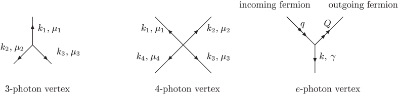
Figure 1: Fermion-, 3-, and 4- photon vertices of noncommutative U(1) theory.

3 Noncommutative Photon Recursion Relation

As noted, noncommutative QED is involved by self-interaction of photons, making it in this respect very similar to a non-Abelian gauge theory. Here we present the photon recursion relations for noncommutative QED. As we will show the general structure of these relations is similar to QCD’s one, though due to appearance of momentum-dependent factors in vertex functions, instead of color ones in QCD case, a special treatment is needed to manage and reexamine the whole machinery in this case. In this section we shall consider the tree-level diagrams involved solely by photons. Consider the matrix element for the diagram with $n+1$ outgoing photons, in the case that one of them is off-shell. This quantity, like its counterpart in QCD case, will be called an $n$-photon current and is denoted by $\widehat{J}_{\xi}(1,2,\cdots,n)$, where $\xi$ denotes the vector index of the off-shell photon. The $(n+1)$-particle amplitude can be obtained from $\widehat{J}_{\xi}(1,2,\cdots,n)$ by a suitable contraction with a polarization vector of the last photon, the $(n+1)\,$th one.

First let us introduce some parts of the notation hereafter are in use. Following the case for QCD, we also define the un-hatted $J_{\xi}(1,2,\cdots,n)$, which essentially defined for the same quantity as $\widehat{J}_{\xi}(1,2,\cdots,n)$, apart from the $\sin(\wedge)$ and $\cos(\wedge)$ factors; in the QCD case the difference between $J$ and $\widehat{J}$ is coming from the color factors [2]. Hence the helicity’s content of current is included only in $J_{\xi}(1,2,\cdots,n)$. We define the sum of momenta $\kappa(i,j)=k_{i}+\cdots+k_{j}$ with $i<j$ [2]. Also, we use the replacement $k_{i}\!\wedge\!(k_{j}+\cdots+k_{n})\to i\!\wedge\!j\cdots n$.

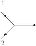
Figure 2: Diagram involving two photons and a third off-shell.

We start with the cases with one, two and three photons. For one photon we simply define

$$\widehat{J}_{\xi}(1)=\epsilon_{\xi}=J_{\xi}(1)$$ (13)

where $\epsilon_{\xi}$ is the polarization vector of the photon, depending on the helicity and momentum $k_{i}$ of the particle. Obviously we have $k_{1}\cdot J(1)=0$. For two photons (see Fig 2) we use the 3-vertex and introduce a propagator

$$\widehat{J}_{\xi}(1,2) = \frac{2ie\sin(1\!\wedge\!2)}{(k_{1}+k_{2})^{2}}\Gamma^{\alpha_{1}\alpha_{2}}_{\xi}\big{(}k_{1},k_{2},-(k_{1}+k_{2})\big{)}J_{\alpha_{1}}(1)J_{\alpha_{2}}(2)$$ (14)

$$= 2ie\frac{\sin(1\!\wedge\!2)}{(k_{1}+k_{2})^{2}}\big{(}2k_{2}\cdot J(1)J_{\xi}(2)-2k_{1}\cdot J(2)J_{\xi}(1)$$

$$+(k_{1}-k_{2})_{\xi}J(1)\cdot J(2)\big{)}$$

As noted earlier we introduce

$$J_{\xi}(1,2) = \frac{1}{(k_{1}+k_{2})^{2}}\big{(}2k_{2}\cdot J(1)J_{\xi}(2)-2k_{1}\cdot J(2)J_{\xi}(1)$$ (15)

$$+(k_{1}-k_{2})_{\xi}J(1)\cdot J(2)\big{)}$$

for which we have

$$(k_{1}+k_{2})\cdot J(1,2) = \frac{1}{(k_{1}+k_{2})^{2}}\big{(}2k_{2}\cdot J(1)J(2)\cdot k_{1}-2k_{1}\cdot J(2)J(1)\cdot k_{2}$$ (16)

$$+(k_{1}+k_{2})\cdot(k_{1}-k_{2})_{\xi}J(1)\cdot J(2)\big{)}$$

$$= (k_{1}^{2}-k_{2}^{2})J(1)\cdot J(2)=0$$

and

$$J_{\xi}(2,1) = \frac{1}{(k_{2}+k_{1})^{2}}\big{(}2k_{1}\cdot J(2)J_{\xi}(1)-2k_{2}\cdot J(2)J_{\xi}(1)$$ (17)

$$+(k_{2}-k_{1})_{\xi}J(2)\cdot J(1)\big{)}$$

$$= \frac{-1}{(k_{1}+k_{2})^{2}}\big{(}2k_{2}\cdot J(1)J_{\xi}(2)-2k_{1}\cdot J(1)J_{\xi}(2)$$

$$+(k_{1}-k_{2})_{\xi}J(1)\cdot J(2)\big{)}=-J_{\xi}(1,2)$$

So we have both of $(k_{1}+k_{2})\cdot J(1,2)=0$, and $J_{\xi}(1,2)=-J_{\xi}(2,1)$. By this we can write

$$\widehat{J}_{\xi}(1,2)=ie\sum_{P(1,2)}\sin(1\!\wedge\!2)J_{\xi}(1,2)$$ (18)

with a sum over the permutations of 1 and 2. We also can introduce new notation by using of commutator symbol

$$J_{\xi}(1,2)=\frac{1}{(k_{1}+k_{2})^{2}}[J(1),J(2)]_{\xi}$$ (19)

where [2]

$$[J(1),J(2)]_{\xi}\!\! = \!\!\Gamma^{\mu_{1}\mu_{2}}_{\xi}\big{(}k_{1},k_{2},-(k_{1}+k_{2})\big{)}J_{\mu_{1}}(1)J_{\mu_{2}}(2)$$ (20)

$$= \!\!\big{(}2k_{2}\cdot J(1)J_{\xi}(2)-2k_{1}\cdot J(2)J_{\xi}(1)+(k_{1}-k_{2})_{\xi}J(1)\cdot J(2)\big{)}$$

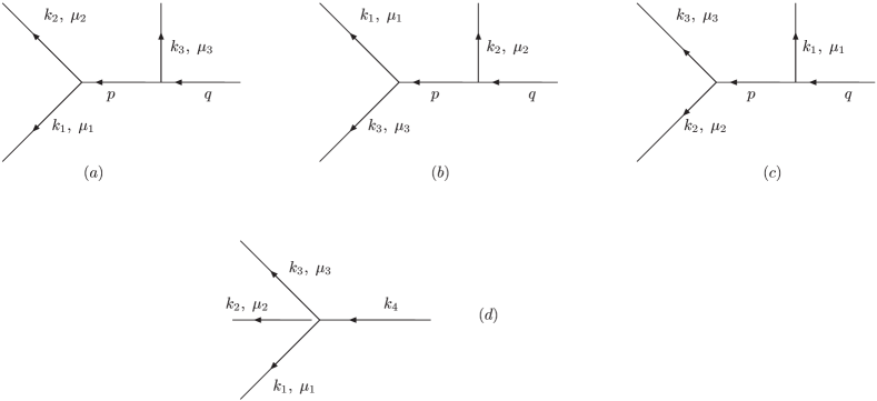
Figure 3: Diagrams contributing in current for three photons.

Now we come to the case with three photons, which is represented by four diagrams (Fig 3). The contribution of diagrams $(a)$-$(c)$ are given by

$$\Gamma^{\rangle{\longrightarrow}{{}^{\mid}}}_{\xi}=\frac{(2ie)^{2}}{\kappa^{2}(1,3)} \!\!\!\!\!\!\Big{(}\sin(3\!\wedge\!12)\sin(1\!\wedge\!2)[J(3),J(1,2)]_{\xi}$$ (21)

$$+\sin(1\!\wedge\!23)\sin(2\!\wedge\!3)[J(1),J(2,3)]_{\xi}$$

$$+\sin(2\!\wedge\!31)\sin(3\!\wedge\!1)[J(2),J(3,1)]_{\xi}\Big{)}$$

in which, for example

$$[J(1),J(2,3)]_{\xi}\!\! = \!\!\Gamma^{\mu_{1}\mu_{2}}_{\xi}\big{(}k_{1},(k_{2}+k_{3}),-(k_{1}+k_{2}+k_{3})\big{)}J_{\mu_{1}}(1)J_{\mu_{2}}(2,3)$$ (22)

$$= \!\!\big{(}2(k_{2}+k_{3})\cdot J(1)J_{\xi}(2,3)-2k_{1}\cdot J(2,3)J_{\xi}(1)$$

$$+(k_{1}-(k_{2}+k_{3}))_{\xi}J(1)\cdot J(2,3)\big{)}$$

By using the identity $2\sin a\sin b=\cos(a-b)-\cos(a+b)$, and the definition $W_{\xi}(i,jk)=\displaystyle{\frac{1}{\kappa^{2}(1,3)}}[J(i),J(j,k)]_{\xi}$, we find

$$\Gamma^{\rangle{\longrightarrow}{{}^{\mid}}}_{\xi}=-2e^{2} \!\!\!\!\!\Big{(}\cos(1\!\wedge\!2+1\!\wedge\!3+2\!\wedge\!3)\,(W(3,12)-W(1,23))_{\xi}$$ (23)

$$+\cos(2\!\wedge\!3+2\!\wedge\!1+3\!\wedge\!1)\,(W(1,23)-W(2,31))_{\xi}$$

$$+\cos(3\!\wedge\!1+1\!\wedge\!2+3\!\wedge\!2)\,(W(2,31)-W(3,12))_{\xi}\Big{)}$$

$W$’s satisfy the following identities,

$$W(i,jk)=-W(jk,i),\;\;W(i,jk)=W(kj,i),\;\;W(i,jk)=-W(i,kj)$$ (24)

by which we find

$$\Gamma^{\rangle{\longrightarrow}{{}^{\mid}}}_{\xi}=e^{2}\sum_{P(1,2,3)}\cos(1\!\wedge\!2+1\!\wedge\!3+2\!\wedge\!3)\,(W(12,3)+W(1,23))_{\xi}$$ (25)

in which sum is over permutations of $(1,2,3)$.

For the seagull diagram Fig 3$(d)$ we have

$$\Gamma^{\;\;\rangle{\longrightarrow}}_{\xi}=\frac{-4e^{2}}{\kappa^{2}(1,3)}\!\!\!\! \Big{(}\sin(1\!\wedge\!2)\sin(3\!\wedge\!4)(J(1)\cdot J(3)J_{\xi}(2)-J(2)\cdot J(3)J_{\xi}(1))$$

$$+\sin(2\!\wedge\!3)\sin(2\!\wedge\!4)(J(1)\cdot J(2)J_{\xi}(3)-J(1)\cdot J(3)J_{\xi}(2))$$

$$+\sin(3\!\wedge\!1)\sin(2\!\wedge\!4)(J(2)\cdot J(3)J_{\xi}(1)-J(2)\cdot J(1)J_{\xi}(3))\Big{)}$$

By definition $I^{i}_{jk,\xi}=J(i)\cdot(J(j)J_{\xi}(k)-J(k)J_{\xi}(j))$ we have

$$\Gamma^{\;\;\rangle{\longrightarrow}}=\frac{-2e^{2}}{\kappa^{2}(1,3)}\!\!\!\! \Big{(}\cos(1\!\wedge\!2+1\!\wedge\!3+2\!\wedge\!3)(I^{3}_{12}-I^{1}_{23})_{\xi}$$ (27)

$$+\cos(2\!\wedge\!3+2\!\wedge\!1+3\!\wedge\!1)(I^{1}_{23}-I^{2}_{31})_{\xi}$$

$$+\cos(3\!\wedge\!1+1\!\wedge\!2+3\!\wedge\!2)(I^{2}_{31}-I^{3}_{12})_{\xi}\Big{)}$$

and by using the cyclic properties of $I^{i}_{jk,\xi}$ one finds

$$\Gamma^{\;\;\rangle{\longrightarrow}}_{\xi}=\frac{-e^{2}}{\kappa^{2}(1,3)}\sum_{P(1,2,3)}\cos(1\!\wedge\!2+1\!\wedge\!3+2\!\wedge\!3)(I^{3}_{12}-I^{1}_{23})_{\xi}$$ (28)

By adding the two contributions of four diagrams we will find:

$$\widehat{J}_{\xi}(1,2,3) = e^{2}\sum_{P(1,2,3)}\cos(1\!\wedge\!2+1\!\wedge\!3+2\!\wedge\!3)\,(W(12,3)+W(1,23))$$ (30)

$$+\frac{e^{2}}{\kappa^{2}(1,3)}\sum_{P(1,2,3)}\cos(1\!\wedge\!2+1\!\wedge\!3+2\!\wedge\!3)(-I^{3}_{12}+I^{1}_{23})_{\xi}$$

$$= \frac{e^{2}}{\kappa^{2}(1,3)}\sum_{P(1,2,3)}\cos(1\!\wedge\!2+12\!\wedge\!3)\,\Big{(}[J(1,2),J(3)]_{\xi}+[J(1),J(2,3)]_{\xi}$$

$$+\{J(1),J(2),J(3)\}_{\xi}\Big{)}$$

in which $\{J(1),J(2),J(3)\}_{\xi}=(I^{1}_{23}-I^{3}_{12})_{\xi}$. One may write in the form

$$\widehat{J}_{\xi}(1,2,3)=e^{2}\sum_{P(1,2,3)}\cos{(1\!\wedge\!2+12\!\wedge\!3)}\;J_{\xi}(1,2,3)$$ (31)

in which

$$J_{\xi}(1,2,3)=\frac{1}{\kappa^{2}(1,3)}\Big{(}[J(1,2),J(3)]+[J(1),J(2,3)]+\{J(1),J(2),J(3)\}\Big{)}_{\xi}$$ (32)

One may, as done for $J_{\xi}(1,2)$, show the following identities for the current $J_{\xi}(1,2,3)$:

$$J(3,2,1)=J(1,2,3)$$

$$J(1,2,3)+J(2,3,1)+J(3,1,2)=0$$

$$\kappa(1,3)\cdot J(1,2,3)=0$$ (33)

Now one may try to present the expression for the current $J_{\xi}$ for the case with $n$ photons. In fact this expression would be the generalization of (32). Here we first suggest an expression, and do prove it by induction. We start with

$$\widehat{J}_{\xi}(1,2,\cdots,n)=(-1)^{n}(ie)^{n-1}\sum_{P(1,\cdots,n)}\;C(123\cdots n;+\frac{n-3}{2}\pi)J_{\xi}(1,\cdots,n)$$ (34)

in which

$$C(123\cdots n;+\frac{n-3}{2}\pi)=\cos\Big{(} \!\!\!\!\!\!\!\!\!\!1\!\wedge\!23\cdots n+2\!\wedge\!34\cdots n+\cdots$$

$$+(n-2)\!\wedge\!(n-1)n+(n-1)\!\wedge\!n+\frac{n-3}{2}\pi\Big{)}$$

or in the case

$$C(123\cdots n;)=\cos\Big{(} \!\!\!\!\!\!\!\!\!\!1\!\wedge\!23\cdots n+2\!\wedge\!34\cdots n+\cdots$$ (36)

$$+(n-2)\!\wedge\!(n-1)n+(n-1)\!\wedge\!n\Big{)}$$

Then a generalization of (32) for $J_{\xi}$ can be

$$J_{\xi}(1,\cdots,n) = \frac{1}{\kappa^{2}(1,n)}\Big{(}\sum_{m=1}^{n-1}[J(1,\cdots,m),J(m+1,\cdots,n)]_{\xi}$$

$$+\sum_{m=1}^{n-2}\sum_{k=m+1}^{n-1}\{J(1,\cdots,m),J(m+1,\cdots,k),J(k+1,\cdots,n)\}_{\xi}\Big{)}$$

This current satisfy the identities

$$(a) \kappa(1,n)\cdot J(1,\cdots,n)=0$$

$$(b) \ J(1,\cdots,n)=(-)^{n-1}J(n,\cdots,1)$$

$$(c) \sum_{Cyc(1,\cdots,n)}J(1,\cdots,n)=0$$ (38)

in which $Cyc(1,\cdots,n)$ is for cyclic permutation on $(1,\cdots,n)$.

One easily can check that for the case $n=1,2,3$ we simply recover the previous expressions. Now we proceed to prove the suggested expression by induction. Let us assume that the expression is valid for any $m$ with $m<n$. Any current for $n$ photons, just like the case for QCD [2], is constructed from considering a 3-vertex and a 4-vertex with all possible currents attached, here might be called generalized 3-vertex and 4-vertex photons, represented by $\Gamma_{\xi}^{1\cdots n,{\rangle{\longrightarrow}}}$ and $\Gamma_{\xi}^{1\cdots n,\;\,{\rangle{\longrightarrow}}}$. By this the starting point the expression [2]

$$\widehat{J}_{\xi}(1,\cdots,n) = \frac{1}{\kappa^{2}(1,n)}\sum_{P(1,\cdots,n)}\Big{(}\sum_{m=1}^{n-1}\frac{1}{2!}\frac{1}{m!}\frac{1}{(n-m)!}\Gamma_{\xi}^{1\cdots m,m+1\cdots n,{\rangle{\longrightarrow}}}$$ (39)

$$\sum_{m=1}^{n-2}\sum_{k=m+1}^{n-1}\frac{1}{3!}\frac{1}{m!}\frac{1}{(k-m)!}\frac{1}{(n-k)!}\Gamma_{\xi}^{1\cdots m,m+1\cdots k,k+1\cdots n,\;\;{\rangle{\longrightarrow}}}\Big{)}$$

In (39) the summation is over all permutations of $n$ photons. In order to avoid multiple counting factors like $\frac{1}{m!}$ are introduced, since $\widehat{J}(1,\cdots,m)$ containing all $m!$ permutation of the particles. Besides we performed breaks in indices $(1,\cdots,n)$ of $\Gamma$’s according to the momentum flow [2]

• In $\Gamma_{\xi}^{1\cdots n,{\rangle{\longrightarrow}}}$, the momenta of photons $1,\cdots,m$ are going through one of legs of $\rangle{\longrightarrow}$, and those of other $m+1,\cdots,n$ ones go through the other left leg.

• In $\Gamma_{\xi}^{1\cdots n,\;\,{\rangle{\longrightarrow}}}$, the momenta of photons $1,\cdots,m$, $m+1,\cdots,k$, and $k+1,\cdots,n$ are going through each left legs of $\big{\rangle{\longrightarrow}}$.

According to the momentum flow above, we would like to introduce a new set of notations for referring the photons belonging to different legs of $\rangle{\longrightarrow}$ and $\big{\rangle{\longrightarrow}}$. We use $(\alpha,\beta)$ for photons $((1,\cdots,m),(m+1,\cdots,n))$ flowing in left legs of $\big{\rangle{\longrightarrow}}$, and $(\alpha,\beta,\gamma)$ for photons $((1,\cdots,m),(m+1,\cdots,k),(k+1,\cdots,n))$ flowing in left legs of $\big{\rangle{\longrightarrow}}$. By these we have the following for $\big{\rangle{\longrightarrow}}$ as examples:

$$\sin(\alpha\!\wedge\!\beta)=\sin\big{(}(1+\cdots+m)\!\wedge\!((m+1)+\cdots+n)\big{)}$$ (40)

As further illustration, by $J(\alpha)$ we mean $J(1,\cdots,m)$. Also we slightly extend the use of symbol “ ; ” in (3) and (36), in the way that here “ ; ” does the same thing in “ $1\cdots n;$ ” here with sets $\alpha$, $\beta$ and $\gamma$. By this we have

$$\alpha\beta;=\alpha\!\wedge\!\beta=(1+\cdots+m)\!\wedge\!((m+1)+\cdots+n)$$

$$\alpha\beta\gamma;=\alpha\!\wedge\!\beta\gamma+\beta\!\wedge\!\gamma$$ (41)

in which by the convention given in the beginning of this section, $\beta\gamma=\beta+\gamma$. In occasion, we may use each of $\alpha$, $\beta$ and $\gamma$, in powers and other places, as numbers. As an example, in $\Gamma^{1\cdots m,m+1\cdots k,k+1\cdots n,\;\;{\rangle{\longrightarrow}}}$, $\alpha$, $\beta$ and $\gamma$ as numbers are simply $m$, $k-m$ and $n-k$, respectively. By these together, relation like $(b)$ of (38) is written as

$$J(\beta)\mid_{P(\beta)}\longrightarrow(-)^{\beta-1}J(\beta)$$ (42)

Now, we can write the generalized 3-vertex function from (20)

$$\Gamma_{\xi}^{\alpha,\beta\{\rangle{\longrightarrow}\}} = ie\sum_{P(\{\alpha\},\{\beta\})}\sin(\alpha\beta;)[\widehat{J}(\alpha),\widehat{J}(\beta)]_{\xi}$$ (43)

$$= ie\sum_{P(\{\alpha\},\{\beta\})}(-)^{\alpha+\beta}(ie)^{\alpha+\beta-2}\sum_{P(1,\cdots,m)}\sum_{P(m+1,\cdots,n)}\sin{(\alpha\beta;)}$$

$$C(\alpha;+\frac{m-3}{2}\pi)C(\beta;+\frac{n-m-3}{2}\pi)[J(\alpha),J(\beta)]_{\xi}$$

$$= ie\sum_{P(\{\alpha\},\{\beta\})}(-)^{\alpha+\beta}(ie)^{\alpha+\beta-2}\sum_{P(1,\cdots,m)}\sum_{P(m+1,\cdots,n)}$$

$$\Big{(}\cos(\alpha;-\beta;+\beta\alpha;+\frac{\alpha-3}{2}\pi-\frac{\beta-3}{2}\pi+\frac{\pi}{2})$$

$$+\cos(\alpha;+\beta;+\beta\alpha;+\frac{\alpha-3}{2}\pi+\frac{\beta-3}{2}\pi-\frac{\pi}{2})$$

$$-\cos(\alpha;-\beta;+\alpha\beta;+\frac{\alpha-3}{2}\pi-\frac{\beta-3}{2}\pi+\frac{\pi}{2})$$

$$-\cos(\alpha;+\beta;+\alpha\beta;+\frac{\alpha-3}{2}\pi+\frac{\beta-3}{2}\pi+\frac{\pi}{2})\Big{)}[J(\alpha),J(\beta)]_{\xi}$$

First we notice, by the interchange $\alpha\leftrightarrow\beta$, that

$$\cos{(\alpha;+\beta;+\beta\alpha;+\frac{\alpha-3}{2}\pi+\frac{\beta-3}{2}\pi-\frac{\pi}{2})}\times[J(\alpha),J(\beta)]\longrightarrow$$

$$-\cos{(\beta;+\alpha;+\alpha\beta;+\frac{\alpha+\beta-3}{2}\pi)}\times[J(\beta),J(\alpha)]$$

$$=-\cos{(\beta;+\alpha;+\alpha\beta;+\frac{\alpha+\beta-3}{2}\pi)}\times(-[J(\alpha),J(\beta)])$$

$$=\cos{(\alpha;+\beta;+\alpha\beta;+\frac{\alpha+\beta-3}{2}\pi)}\times[J(\alpha),J(\beta)]$$ (44)

Similarly, by $\alpha\leftrightarrow\beta$ and then doing permutation among $\alpha$’s members, we get

$$\cos{(\alpha;-\beta;+\beta\alpha;+\frac{\alpha-3}{2}\pi-\frac{\beta-3}{2}\pi+\frac{\pi}{2})}\times[J(\alpha),J(\beta)]\longrightarrow$$

$$=\cos{(\beta;+\alpha;+\beta\alpha;+\frac{\beta-3}{2}\pi-\frac{\alpha-3}{2}\pi+\frac{\pi}{2})}\times[J(\beta),J(\alpha)](-)^{\alpha-1}$$

$$=\cos{(\alpha;+\beta;+\alpha\beta;+\frac{\alpha-3}{2}\pi+\frac{\beta-3}{2}\pi-(\alpha-3)\pi+\frac{\pi}{2})}\times[J(\beta),J(\alpha)](-)^{\alpha-1}$$

by which, no matter $\alpha$ is even or odd, we get

$$\cos{(\alpha;+\beta;+\alpha\beta;+\frac{\alpha-3}{2}\pi+\frac{\beta-3}{2}\pi-(\alpha-3)\pi+\frac{\pi}{2})}\times[J(\beta),J(\alpha)](-)^{\alpha-1}$$

$$=\cos{(\alpha;+\beta;+\alpha\beta;+\frac{\alpha+\beta-3}{2}\pi)}\times[J(\alpha),J(\beta)]$$ (46)

Lastly we have

$$-\cos{(\alpha;-\beta;+\alpha\beta;+\frac{\alpha-3}{2}\pi-\frac{\beta-3}{2}\pi+\frac{\pi}{2})}\times[J(\alpha),J(\beta)]\longrightarrow$$

$$=-\cos{(\alpha;+\beta;+\alpha\beta;+\frac{\alpha-3}{2}\pi-\frac{\beta-3}{2}\pi+\frac{\pi}{2})}\times[J(\alpha),J(\beta)](-)^{\beta-1}$$

$$=\cos{(\alpha;+\beta;+\alpha\beta;+\frac{\alpha+\beta-3}{2}\pi)}\times[J(\alpha),J(\beta)]$$ (47)

Using these all the generalized 3-vertex current is given by

$$\widehat{J}(1,\cdots,n)|_{{}_{\big{\rangle{\longrightarrow}{{}^{\mid}}}}}=(-)^{n}(ie)^{n-1}\sum_{P(1,\cdots,n)}C(1\cdots n;+\frac{n-3}{2}\pi)J(1,\cdots,n)$$ (48)

in which

$$J(1,\cdots,n)=\frac{1}{\kappa^{2}(1,n)}\sum_{m=1}^{n-1}[J(1,\cdots,m),J(m+1,\cdots,n)]$$ (49)

For the 4-vertex term we have

$$\Gamma^{\alpha,\beta,\gamma,\{\;\;\rangle{\longrightarrow}\}}_{\xi} = -4e^{2}\Big{(}\sin{(\alpha\beta;)}\sin{(\gamma\!\wedge\!(\alpha+\beta+\gamma))}$$ (50)

$$\times(\widehat{J}(\alpha)\cdot\widehat{J}(\gamma)\widehat{J}_{\xi}(\beta)-\widehat{J}(\beta)\cdot\widehat{J}(\gamma)\widehat{J}_{\xi}(\alpha))$$

$$+\sin{(\beta\gamma;)}\sin{(\alpha\!\wedge\!(\alpha+\beta+\gamma))}$$

$$\times(\widehat{J}(\alpha)\cdot\widehat{J}(\beta)\widehat{J}_{\xi}(\gamma)-\widehat{J}(\alpha)\cdot\widehat{J}(\gamma)\widehat{J}_{\xi}(\beta))$$

$$+\sin{(\gamma\alpha;)}\sin{(\beta\!\wedge\!(\alpha+\beta+\gamma))}$$

$$\times(\widehat{J}(\beta)\cdot\widehat{J}(\gamma)\widehat{J}_{\xi}(\alpha)-\widehat{J}(\beta)\cdot\widehat{J}(\alpha)\widehat{J}_{\xi}(\gamma))\Big{)}$$

By the definition $\widehat{I}^{\alpha}_{\beta\gamma\xi}=\widehat{J}(\alpha)\cdot(\widehat{J}(\beta)\widehat{J}_{\xi}(\gamma)-\widehat{J}(\gamma)\widehat{J}_{\xi}(\beta))$, and using the relations

$$2\sin{(\gamma\!\wedge\!(\alpha+\beta+\gamma))}\sin{(\alpha\beta;)} = \cos(\alpha\beta;+\alpha\gamma;+\beta\gamma;)$$ (51)

$$-\cos(\alpha\beta;+\gamma\alpha;+\gamma\beta;)$$

we can write

$$\Gamma^{\alpha,\beta,\gamma,\{{\;\;\rangle{\longrightarrow}}\}}_{\xi}=-2e^{2} \!\!\!\!\!\!\!\!\!\Big{(}\cos(\alpha\beta;+\alpha\gamma;+\beta\gamma;)(\widehat{I}^{\gamma}_{\alpha\beta}-\widehat{I}^{\alpha}_{\beta\gamma})_{\xi}$$ (52)

$$\!\!\!\!\!\!\!\!\!+\cos(\beta\gamma;+\beta\alpha;+\gamma\alpha;)(\widehat{I}^{\alpha}_{\beta\gamma}-\widehat{I}^{\beta}_{\gamma\alpha})_{\xi}$$

$$\!\!\!\!\!\!\!\!\!+\cos(\gamma\alpha;+\alpha\beta;+\gamma\beta;)(\widehat{I}^{\beta}_{\gamma\alpha}-\widehat{I}^{\gamma}_{\alpha\beta})_{\xi}\Big{)}$$

which can be written in a shorten way

$$\Gamma^{\alpha,\beta,\gamma,\{{\;\;\rangle{\longrightarrow}}\}}=-e^{2}\sum_{P(\{\alpha\},\{\beta\},\{\gamma\})}\cos{(\alpha\beta\gamma;)}(\widehat{I}^{\gamma}_{\alpha\beta}-\widehat{I}^{\alpha}_{\beta\gamma})_{\xi}$$ (53)

We introduce $\{\widehat{J}(\alpha),\widehat{J}(\beta),\widehat{J}(\gamma)\}=\widehat{I}^{\alpha}_{\beta\gamma}-\widehat{I}^{\gamma}_{\alpha\beta}$, satisfying

$$\{\widehat{J}(\gamma),\widehat{J}(\beta),\widehat{J}(\alpha)\}=\{\widehat{J}(\alpha),\widehat{J}(\beta),\widehat{J}(\gamma)\}$$ (54)

So (53) becomes

$$\Gamma^{\alpha,\beta,\gamma,\{{\;\;\rangle{\longrightarrow}}\}} = e^{2}(-)^{\alpha+\beta+\gamma}(ie)^{\alpha+\beta+\gamma-3}$$ (55)

$$\sum_{P(1,\cdots,m)}\sum_{P(m+1,\cdots,k)}\sum_{P(k+1,\cdots,n)}\sum_{P(\{\alpha\},\{\beta\},\{\gamma\})}C(\alpha\beta\gamma;)$$

$$C(\alpha;(m-3)\frac{\pi}{2})C(\beta;(k-m-3)\frac{\pi}{2})$$

$$C(\gamma;(n-k-3)\frac{\pi}{2})\{J(\alpha),J(\beta),J(\gamma)\}$$

leading to

$$\Gamma^{\alpha,\beta,\gamma,\{{\;\;\rangle{\longrightarrow}}\}} = e^{2}(-)^{\alpha+\beta+\gamma}(ie)^{\alpha+\beta+\gamma-3}$$ (56)

$$\sum_{P(1,\cdots,m)}\sum_{P(m+1,\cdots,k)}\sum_{P(k+1,\cdots,n)}\sum_{P(\{\alpha\},\{\beta\},\{\gamma\})}$$

$$\frac{1}{8}\Big{(}\cos{(\alpha\beta\gamma;-\alpha;-\beta;-\gamma;-(\frac{n-9}{2}\pi))}$$

$$+\cos{(\alpha\beta\gamma;-\alpha;-\beta;+\gamma;+(\frac{n-2k+3}{2}\pi))}$$

$$+\cos{(\alpha\beta\gamma;-\alpha;+\beta;+\gamma;+(\frac{n-2m-3}{2}\pi))}$$

$$+\cos{(\alpha\beta\gamma;+\alpha;-\beta;-\gamma;-(\frac{n-2m-3}{2}\pi))}$$

$$+\cos{(\alpha\beta\gamma;+\alpha;-\beta;+\gamma;+(\frac{n-2k+2m-3}{2}\pi))}$$

$$+\cos{(\alpha\beta\gamma;+\alpha;+\beta;-\gamma;+(\frac{2k-n-3}{2}\pi))}$$

$$+\cos{(\alpha\beta\gamma;-\alpha;+\beta;-\gamma;-(\frac{n-2k+2m-3}{2}\pi))}$$

$$+\cos{(\alpha\beta\gamma;+\alpha;+\beta;+\gamma;+(\frac{n-9}{2}\pi))}\Big{)}$$

$$\times\{J(\alpha),J(\beta),J(\gamma)\}$$

Like the similar way we should in previous case, by proper interchanges among $\alpha\leftrightarrow\beta\leftrightarrow\gamma\leftrightarrow\alpha$, permutations among $\alpha$’s, $\beta$’s and $\gamma$’s members, and and use of $J(\alpha)\mid_{P(\{\alpha\})}=(-)^{\alpha-1}J(\alpha)$, the eight cosine-terms will be equal to

$$-\cos{(\alpha\beta\gamma;+\alpha;+\beta;+\gamma;+(\frac{n-3}{2}\pi))}\times\{J(\alpha),J(\beta),J(\gamma)\}$$ (57)

So

$$\Gamma^{\alpha,\beta,\gamma,\{{\;\;\rangle{\longrightarrow}}\}} = e^{2}(-)^{\alpha+\beta+\gamma}(ie)^{\alpha+\beta+\gamma-3}$$ (58)

$$\sum_{P(1,\cdots,m)}\sum_{P(m+1,\cdots,k)}\sum_{P(k+1,\cdots,n)}$$

$$\cos{(\alpha\beta\gamma;+\alpha;+\beta;+\gamma;+(\frac{n-9}{2}\pi))}\times\{J(\alpha),J(\beta),J(\gamma)\}$$

$$= (-)^{\alpha+\beta+\gamma}(ie)^{\alpha+\beta+\gamma-1}\sum_{P(1,\cdots,m)}\sum_{P(m+1,\cdots,k)}\sum_{P(k+1,\cdots,n)}$$

$$C(\alpha\beta\gamma;+\frac{n-3}{2}\pi)\times\{J(\alpha),J(\beta),J(\gamma)\}$$

Finally

$$\Gamma^{\{\;\;\rangle{\longrightarrow}\}}=\sum^{n-2}_{m=1}\sum^{n-1}_{k=m+1}\Gamma^{\alpha,\beta,\gamma,\{{\;\;\rangle{\longrightarrow}}\}}$$ (59)

From this, the second term in (34) easily follows.

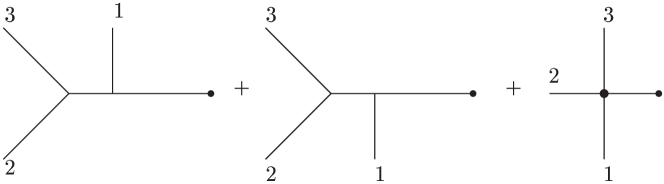
Figure 4: Diagrams have a clock-wise orientation for three photons

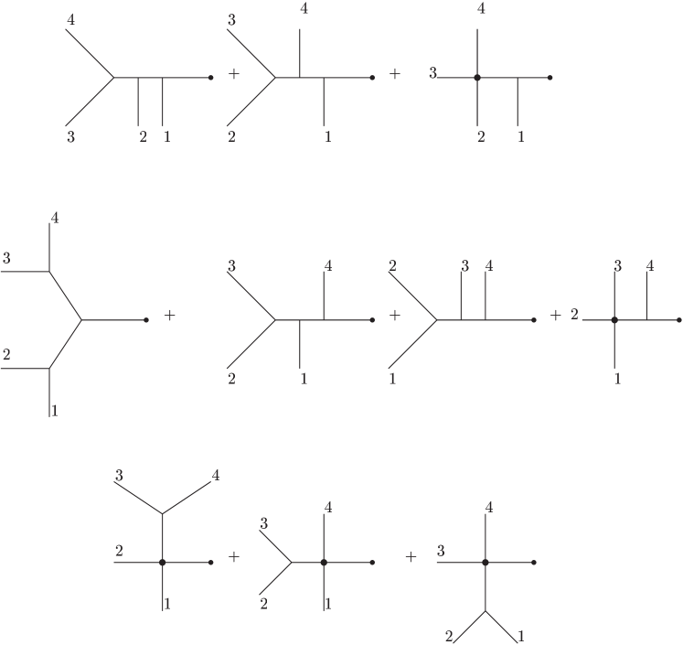
Figure 5: Diagrams have a clock-wise orientation for four photon

The current $J(1,\cdots,n)$ has the properties

$$J(n,n-1,\cdots,1) = (-)^{n-1}J(1,\cdots,n)$$ (60)

$$\sum_{Cyc(1,\cdots,n)}J(1,\cdots,n) = 0$$ (61)

$$\kappa(1,n)\cdot J(1,\cdots,n) = 0$$ (62)

The properties of $J$ is like that are proven in [2]. One may wonder how the $n$-photon current is affected when we change the gauge of specific photon,

$$\widetilde{J}(1)=J(1)+\rho k_{1}$$ (63)

We replace $J_{1}$ by $k_{1}$ in recursion relation and after evaluating the current for a few cases one is led to a general answer for the current with $J_{1}=k_{1}$

$$J(1,\cdots,n)=-\kappa(1,n)\frac{\kappa(1,n)\cdot\acute{J}(2,\cdots,n)}{\kappa^{2}(1,n)}+\acute{J}(2,\cdots,n)$$ (64)

with $\acute{J}(2)=J(2)$,

$$\acute{J}(2,\cdots,n)=J(1,\cdots,n)-\sum_{m=2}^{n-1}\frac{\kappa(1,m)\cdot\acute{J}(2,\cdots,m)}{\kappa^{2}(1,m)}J(m+1,\cdots,n)$$ (65)

Using induction, this form can be proven to be correct. The recursion relation include of clock-wise orientation for the labels $1,2,\cdots,n$ that is number of all diagrams occurring in recursion relation; for three photons there are 3 (Fig 4), and for four photons 10 (Fig 5) [2].

4 Spinorial recursion relations

In this section we derive an expression for the matrix element involving an electron-positron pair and $n$ photons, all outgoing and the positron off-shell. We introduce the spinorial current $\widehat{J}(Q,1,2,\cdots,n)$. In this notation $Q$ stands for the electron’s momentum whereas the electron helicity is suppressed. Moreover $1,2,\cdots,n$ denote the $n$ photons. The spinor index $c$ of the off-shell positron is written explicitly.

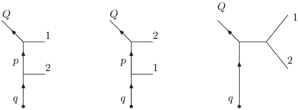
Figure 6: Fermion coupled to two photons

For a single electron and no photon we simply have

$$\widehat{J}(Q)=\bar{u}(Q)=J(Q)$$ (66)

The one photon spinorial current is

$$\widehat{J}(Q,1)=(ie\,{\rm e}^{i1\,\!\wedge\!\,Q})\bar{u}(Q)\epsilon/_{1}\frac{i}{Q\diagup+k\diagup_{1}-m_{0}}=e\,{\rm e}^{i1\,\!\wedge\!\,Q}J(Q,1)$$ (67)

in which $m_{0}$ as electron’s mass, and with

$$J(Q,1)=-J(Q)J\diagup(1)\frac{1}{Q\diagup+k\diagup_{1}-m_{0}}$$ (68)

For two photons we have the contribution of three diagrams (see Fig 6), giving

$$\widehat{J}(Q,1,2) = (\frac{-e}{Q\diagup+k\diagup_{1}+k\diagup_{2}-m_{0}})\Big{(}\,{\rm e}^{i2\,\!\wedge\!\,Q1}\widehat{J}(Q,1)J\diagup(2)$$ (69)

$$+\,{\rm e}^{i1\,\!\wedge\!\,\,Q2}\widehat{J}(Q,2)J\diagup(1)+\,{\rm e}^{i12\,\!\wedge\!\,\,Q}J(Q)\sum_{P(1,2)}\widehat{J\diagup}(1,2)\Big{)}$$

$$= (\frac{-e}{Q\diagup+k\diagup_{1}+k\diagup_{2}-m_{0}})\times\sum_{P(1,2)}\Big{(}\,{\rm e}^{i2\,\!\wedge\!\,Q1}\widehat{J}(Q,1)J\diagup(2)$$

$$+\,{\rm e}^{i12\,\!\wedge\!\,\,Q}J(Q)\widehat{J\diagup}(1,2)\Big{)}$$

$$= (\frac{-e^{2}\,{\rm e}^{i21\,\!\wedge\!\,Q}}{Q\diagup+k\diagup_{1}+k\diagup_{2}-m_{0}})\times\sum_{P(1,2)}\Big{(}\,{\rm e}^{i2\,\!\wedge\!\,1}J(Q,1)J\diagup(2)$$

$$+iJ(Q)\cos(12;-\frac{1}{2}\pi)J\diagup(1,2)\Big{)}$$

Noting that

$$\sum_{P(1,2)}\,{\rm e}^{i12;}J\diagup(1,2)=\sum_{P(1,2)}\,{\rm e}^{-i12;}J\diagup(2,1)$$ (70)

leads one to

$$\widehat{J}(Q,1,2) = (\frac{-e^{2}\,{\rm e}^{i21\!\wedge\!Q}}{Q\diagup+k\diagup_{1}+k\diagup_{2}-m_{0}})$$ (71)

$$\times \sum_{P(1,2)}\,{\rm e}^{i2\,\!\wedge\!\,1}\Big{(}J(Q,1)J\diagup(2)+\frac{i}{2}J(Q)(-\,{\rm e}^{-i\frac{1}{2}\pi}+\,{\rm e}^{i\frac{1}{2}\pi})J\diagup(1,2)\Big{)}$$

It is convenient to introduce the abbreviation $K=(k_{1},\cdots,k_{n})$ for all $k_{i}$’s as photons’ momenta. Then, reminding the action of “ ; ” from previous section, we can write:

$$\widehat{J}(Q,1,2)=e^{2}\sum_{P(1,2)}\,{\rm exp}(iKQ;-iK;)J(Q,1,2)$$ (72)

with

$$\exp(iKQ;-iK;)=\exp\big{(}i(12\cdots n)\!\wedge\!Q-i(12\cdots n;)\big{)}$$ (73)

and

$$J(Q,1,2)=\frac{-1}{Q\diagup+k\diagup_{1}+k\diagup_{2}-m_{0}}(J(Q,1)J\diagup(2)+\frac{i}{2}J(Q)(-\,{\rm e}^{-i\frac{1}{2}\pi}+\,{\rm e}^{i\frac{1}{2}\pi})J\diagup(1,2))$$ (74)

To express the relation for arbitrary $n$ we need to go one more step, to find the current for $n=3$ photons, given by

$$\widehat{J}(Q,1,2)\widehat{J\diagup}(3)+\widehat{J}(Q,1)\widehat{J\diagup}(2,3)+\widehat{J}(Q)\widehat{J\diagup}(1,2,3)=\frac{\mathbb{A}+\mathbb{B}+\mathbb{C}}{Q\diagup+\kappa\diagup(1,3)-m_{0}}$$ (75)

The task is now to find $\mathbb{A}$, $\mathbb{B}$ and $\mathbb{C}$,

$$\mathbb{A} = -e\sum_{Cyc(1,2,3)}\,{\rm e}^{i3\,\!\wedge\!\,\,Q12}\widehat{J}(Q,1,2)J\diagup(3)$$ (76)

$$= -e\sum_{Cyc(1,2,3)}\,{\rm e}^{i3\,\!\wedge\!\,Q12}\{e^{2}\,{\rm e}^{i12\,\!\wedge\!\,\,Q}\sum_{P(1,2)}\,{\rm e}^{i2\,\!\wedge\!\,1}J(Q,1,2)\}J\diagup(3)$$

$$= -e^{3}\sum_{P(1,2,3)}\,{\rm e}^{i321\,\!\wedge\!\,Q+i32\,\!\wedge\!\,12}J(Q,1,2)J\diagup(3)$$

$$= -e^{3}\sum_{P(1,2,3)}\,{\rm exp}(iKQ;-iK;)J(Q,1,2)J\diagup(3)$$

Then we have

$$\mathbb{B} = -e\sum_{Cyc(1,2,3)}\,{\rm e}^{i32\,\!\wedge\!\,\,Q1}\widehat{J}(Q,1)\widehat{J\diagup}(2,3)$$ (77)

$$= -e\sum_{Cyc(1,2,3)}\,{\rm e}^{i32\,\!\wedge\!\,Q1}\{e\,{\rm e}^{i1\,\!\wedge\!\,\,Q}J(Q,1)\sum_{P(2,3)}(+ie\cos(23;-\frac{\pi}{2}))J\diagup(2,3)\}$$

$$= -ie^{3}\sum_{Cyc(1,2,3)}\,{\rm e}^{i321\,\!\wedge\!\,Q+i32\,\!\wedge\!\,1}J(Q,1)\sum_{P(2,3)}(\frac{\,{\rm e}^{i2\,\!\wedge\!\,3-i\frac{\pi}{2}}+\,{\rm e}^{-i2\,\!\wedge\!\,3+i\frac{\pi}{2}}}{2})J\diagup(2,3)$$

$$= -ie^{3}\sum_{P(1,2,3)}\frac{1}{2}\,{\rm e}^{i321\,\!\wedge\!\,\,Q+i32\,\!\wedge\!\,21}J(Q,1)(\,{\rm e}^{i\frac{1}{2}\pi}J\diagup(2,3)+\,{\rm e}^{-i\frac{1}{2}\pi}J\diagup(3,2))$$

$$= -ie^{3}\sum_{P(1,2,3)}\frac{1}{2}\,{\rm e}^{i321\,\!\wedge\!\,\,Q+i32\,\!\wedge\!\,21}J(Q,1)(\,{\rm e}^{i\frac{1}{2}\pi}-\,{\rm e}^{-i\frac{1}{2}\pi})J\diagup(2,3)$$

Lastly we have

$$\mathbb{C} = -e\,{\rm e}^{i321\,\!\wedge\!\,\,Q}\widehat{J}(Q)\widehat{J\diagup}(1,2,3)$$ (78)

$$= -e^{3}\,{\rm e}^{i321\,\!\wedge\!\,\,Q}J(Q)\sum_{P(1,2,3)}C(123;)J\diagup(1,2,3)$$

Based on the expressions coming from previous section, we have

$$\sum_{P(1,\cdots,n)}C(1\cdots n;\frac{n-3}{2}\pi)J_{\xi}(1,\cdots,n)$$

$$=\frac{1}{2}\sum_{P(1,\cdots,n)}\exp(-iK;)\,(\,{\rm e}^{i\frac{n-3}{2}\pi}J_{\xi}(n,\cdots,1)+\,{\rm e}^{-i\frac{n-3}{2}\pi}J_{\xi}(1,\cdots,n))$$

$$=\frac{1}{2}\sum_{P(1,\cdots,n)}\exp(-iK;)(\,{\rm e}^{i\frac{n-3}{2}\pi}(-)^{n-1}+\,{\rm e}^{-i\frac{n-3}{2}\pi})J_{\xi}(1,\cdots,n)$$ (79)

by which we finally reach to

$$\mathbb{C}=-e^{3}\sum_{P(1,2,3)}\exp(iKQ;-iK;)J(Q)\times J\diagup(1,2,3)$$ (80)

Now we express the general form of spinorial current for the case with $n$ photons

$$\widehat{J}(Q,1,\cdots,n)=e^{n}\sum_{P(1,\cdots,n)}\exp(iKQ;-iK;)J(Q,1,\cdots,n)$$ (81)

where

$$J(Q,1,\cdots,n)=\frac{-1}{Q\diagup+\kappa\diagup(1,n)-m_{0}}\sum_{m=0}^{n-1}h(n,m)J(Q,1,\cdots,m)J\diagup(m+1,\cdots,n)$$ (82)

in which

$$h(n,m)=\frac{1}{2}(-)^{n-m}(i)^{n-m-1}(\,{\rm e}^{-i\frac{n-m-3}{2}\pi}+(-)^{n-m-1}\,{\rm e}^{i\frac{n-m-3}{2}\pi})$$ (83)

It will be useful to have a spinorial current where the outgoing fermion instead of the positron is off-shell. The spinorial current with outgoing electron off-shell can be simply obtained. For one positron it is

$$J(P)=v(P)$$ (84)

where $P$ is the positron momentum. One easily can check the following replacements yield the positron currents

$$Q \to -P$$

$$\frac{-1}{Q\diagup+k\diagup(1,n)-m_{0}} \to \frac{1}{P\diagup+k\diagup(1,n)+m_{0}}$$

$$J(Q,1,\cdots,m)J\diagup(m+1,\cdots,n) \to J\diagup(1,\cdots,m)J(m+1,\cdots,n,P)$$

$$h(n,m) \to \tilde{h}(n,m)=\frac{1}{2}(-)^{m}(i)^{m-1}$$ (85)

$$\times((-)^{m-1}\,{\rm e}^{-i\frac{m-3}{2}\pi}+\,{\rm e}^{i\frac{m-3}{2}\pi})$$

Then the positron currents are given by

$$\widehat{J}(1,\cdots,n,P)=e^{n}\sum_{p(1,\cdots,n)}\exp(-iKP;+iK;)J(1,\cdots,n,P)$$ (86)

in which

$$J(1,\cdots,n,P)=\frac{1}{P\diagup+k\diagup(1,n)+m_{0}}\sum_{m=1}^{n}\tilde{h}(n,m)J\diagup(1,\cdots,m)J(m+1,\cdots,n,P)$$ (87)

One can express the relation between two currents by electron and positron by means of charge conjugation operator ${\cal C}$ [2]

$${\cal C}v_{\pm} = -\bar{u}^{T}_{\pm}$$

$$\bar{u}_{\pm}{\cal C}^{-1} = v^{T}_{\pm}$$ (88)

in which $v_{\pm}=\frac{1}{2}(1\mp\gamma_{5})v$ and $u_{\pm}=\frac{1}{2}(1\pm\gamma_{5})u$, and the superscript $T$ for transpose.
Following [17] we know that ${\cal C}$ is a symmetry of noncommutative theory when is accompanied with the change $\theta\rightarrow-\theta$, with $\theta$ as the parameter of noncommutativity.
So by means of the action of ${\cal C}$ the currents are related [2]

$${\cal C}J(1,\cdots,n,P_{\pm})\mid_{\theta}=(-)^{n-1}J^{T}(P_{\pm},n,\cdots,1)\mid_{-\theta}$$ (89)

or

$$J(P_{\pm},1,\cdots,n)\mid_{\theta}\,{\cal C}^{-1}=-(-)^{n-1}J^{T}(1,\cdots,n,P_{\pm})\mid_{-\theta}$$ (90)

in which $\pm$ denote the helicity of outgoing positron or electron.

5 Conclusion

The $n$-photon recursion relations for purely photonic processes of noncommutative QED are derived. Also the same relations are presented for processes with one pair of fermions involved. Although the general structure of these relations for noncommutative QED is similar to QCD’s one, due to appearance of momentum-dependent factors in vertex functions, instead of momentum-independent color ones of QCD, a special treatment is needed to manage and reexamine the whole machinery in this case. The relations can be considered as the first step to employ the recursion relation method for noncommutative QED case.

Acknowledgement: The author is grateful to A. H. Fatollahi for helpful discussions and comments on the manuscript.

References

[1] S. Parke and T. Taylor, Phys. Rev. Lett. 56 (1986) 2459.
[2] F. A. Berends and W. T. Giele, Nucl. Phys. B 306 (1988) 759; Nucl. Phys. B 313
(1989) 595; Nucl. Phys. B 294 (1987) 700.
[3] F. A. Berends, R. Kleiss, P. de Causmaecker, R. Gastmans and T. T. Wu,
Phys. Lett. B 103 (1981) 124; R. Kleiss and W. J. Stirling, Phys. Lett. B 179 (1986) 2459;
R. Kleiss and W. J. Stirling, Nucl. Phys. B 262 (1985) 235; F. A. Berends, R. Kleiss, P. de Causmaecker,
R. Gastmans, W. Troost and T. T. Wu, Nucl. Phys. B 206 (1982) 61; F. A. Berends, P. de Causmaecker,
R. Gastmans, R. Kleiss, W. Troost and T. T. Wu, Nucl. Phys. B 239 (1984) 382; Nucl. Phys. B 239 (1984) 395;
Nucl. Phys. B 264 (1986) 243; Nucl. Phys. B 264 (1986) 265.
[4] D.A. Kosower, Phys. Rev. D 71 (2005) 045007, hep-th/0406175.
[5] L. J. Dixon, E. W. N. Glover and V. Khoze, JHEP 0412 (2004)015, hep-th/0411092;
T. G. Brithwright, E. W. N. Glover, V. Khoze and P. Marquard, JHEP 0505 (2005) 013, hep-ph/0503063.
[6] R. Kleiss and W. J. Stirling, Phys. Lett. B 179 (1986) 159.
[7] F. Cachazo, P. Svrcek and E. Witten, JHEP 0409 (2004) 006, hep-th/0403047.
[8] J.-B. Wu and C.-J. Zhu, JHEP 0407 (2004) 032, hep-th/0406085;
JHEP 0409 (2004) 063, hep-th/0406146; L. J. Dixon, E. W. N. Glover and V. Khoze, JHEP 0412
(2004) 070, hep-th/0411092.
[9] K. J. Ozeren and W. J. Stiriling, JHEP 0511 (2005) 016, hep-th/0509063.
[10] A. Ilderton, Nucl. Phys. B 742 (2006) 176, hep-th/0512007.
[11] R. Britto, F. Cachazo and B. Feng, Nucl. Phys. B 715 (2005) 499, hep-th/0412308.
[12] E. Witten, Commun. Math. Phys. 252 (2004) 189-258,
hep-th/0312171; F. Cachazo and P. Svrcek, PoS RTN2005 (2005)
004, hep-th/0504194; G. Georgiou and V. Khoze, JHEP 0405 (2004)070, hep-th/0404072.
[13] N. Seiberg and E. Witten, JHEP 9909 (1999) 032, hep-th/9908142;
A. Connes, M. R. Douglas, and A. Schwarz, JHEP 9802 (1998) 003, hep-th/9711162;
M. R. Douglas and C. Hull, JHEP 9802 (1998) 008, hep-th/9711165.
[14] M. R. Douglas and N. A. Nekrasov, “Noncommutative Field Theory,”
Rev. Mod. Phys. 73 (2001) 977, hep-th/0106048.
[15] A. H. Fatollahi,
Eur. Phys. J. C 17 (2000) 535, hep-th/0007023;
Phys. Lett. B 512 (2001) 161, hep-th/0103262;
Eur. Phys. J. C 21 (Jul. 2001) 717, hep-th/0104210.
[16] I. F. Riad and M. M. Sheikh-Jabbari, JHEP 0008 (2000) 045, hep-th/0008132.
[17] M. M. Sheikh-Jabbari, Phys. Rev. Lett. 84 (2000) 5265, hep-th/0001167.