Analytic Evidence for Continuous Self Similarity of the Critical Merger Solution

Abstract:

The double cone, a cone over a product of a pair of spheres, is known to play a role in the black-hole black-string phase diagram, and like all cones it is continuously self similar (CSS). Its zero modes spectrum (in a certain sector) is determined in detail, and it implies that the double cone is a co-dimension 1 attractor in the space of those perturbations which are smooth at the tip. This is interpreted as strong evidence for the double cone being the critical merger solution. For the non-symmetry-breaking perturbations we proceed to perform a fully non-linear analysis of the dynamical system. The scaling symmetry is used to reduce the dynamical system from a 3d phase space to 2d, and obtain the qualitative form of the phase space, including a non-perturbative confirmation of the existence of the “smoothed cone”.

1 Introduction and Summary

The phase diagram of the black-hole black-string transition (see the reviews [1, 2]) was conjectured in [3] to include a “merger” point – a static vacuum metric (see figure 1) which lies on the boundary between the black-string and black-hole branches. It can be thought as either a black string whose waist has become so thin that it has marginally pinched, or as a black-hole which has become so large that its poles had marginally intersected and merged (and hence the name “merger”). The metric cannot be completely smooth as it interpolates between two different space-time topologies, but it may have only one naked singularity.

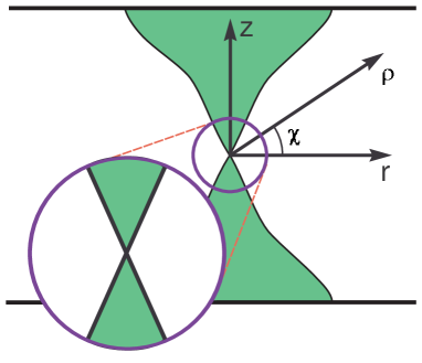
Figure 1: The merger metric. $r$ is the radial coordinate in the extended directions, $z$ is periodically compactified, while time and angular coordinates are suppressed. The heavy lines denote the horizon of a static black object which is at threshold between being a black-hole and being a black-string. The naked singularity is at the $\times$-shaped pinching (horizon crossing) point. Upon zooming onto the encircled singularity it is convenient to replace $(r,z)$ by radial coordinates $(\rho,\chi)$ radial coordinates. We shall be mostly interested in the “critical merger solution” – the local metric near the singularity, namely the encircled portion of the metric (in the limit that the circle’s size is infinitesimal).

The black-hole black-string system has been the subject of intensive numerical research [4, 5, 6, 7, 8]. Naturally, the merger space-time itself is unattainable numerically since it includes a singularity, but it may be approached by following either of the two branches far enough. Indeed, all the available data indicates that the black-string and the black-hole branches approach each other, in accord with the merger prediction.

At merger the curvature is unbounded around the pinch point. One defines the “critical merger solution” to be the local metric around the pinch point (at merger), namely the one achieved through a zooming limit around the point. It is natural to predict [3, 9] that the critical merger solution will lose all memory of the macroscopical scales of the problem (the size of the extra dimension and the size of the black hole) and moreover be self-similar, namely invariant under a scaling transformation. The central motivation of this paper is to determine the critical merger solution.

Self-similar metrics belong to one of two classes: Continuous Self-Similarity (CSS) or Discrete Self-Similarity (DSS): while a CSS metric is invariant under any scale transformation and can be pictured as a cone, a DSS metric is invariant only under a specific scaling transformation (and its powers) and can be pictured as a wiggly cone with its wiggles being log-periodic (see figure 2). A key question is: Is the critical merger solution CSS or DSS?

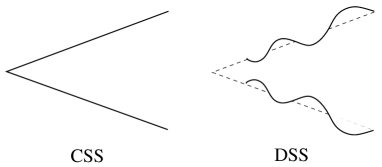
Figure 2: An illustration of a continuously self-similar geometry (CSS) as a cone, and a discretely self-similar geometry (DSS) as a wiggly cone. The singularity is at the tip.

The significance of the critical solution is that critical exponents of the system near the merger point are determined by properties of this solution (this is known to be the case in the closely related system [9] of Choptuik critical collapse [10, 11]).

Considerations and plan. The direct way to settle our question would be through numerical simulation of the system: one would need to obtain solutions which are ever closer to the merger and with ever higher resolution near the high curvature region (where the singularity is about to form). This computation would be comparable in difficulty to Choptuik’s original discovery of critical collapse [10] in that it requires successive mesh refinements over several orders of magnitude.

However, since we are asking a local question, we may expect or hope that a local analysis would suffice, namely the analysis of the metric close to the singularity. On the one hand a local analysis is disadvantaged relative to a solution of the whole system in being indirect and therefore its results need some interpretation which reduces certainty. On the other hand, a local analysis supplies more insight into the mechanism that determines the local metric, and it is easier to perform. These latter advantages induced us to prefer the local analysis for the current study. The demanding full (numerical) analysis is yet to be performed (see however the suggestive but inconclusive results in [12]).

Our first assumption is that the local metric is self-similar, as discussed above. Our second working assumption is that if several self-similar metrics exist then the one actually realized by the system is the metric which is most attractive, or most stable, in an appropriately defined manner.

One local self-similar solution, the “double-cone” has been known for a while [3]. In terms of the $(\rho,\chi)$ coordinates defined in figure 1 it is given by

$$ds^{2}=d\rho^{2}+{1\over D-2}\,\rho^{2}\left[d\chi^{2}+\cos^{2}(\chi)\,dt^{2}+(D-4)\,d\Omega^{2}_{D-3}\right]~{},$$ (1)

where $t$ denotes Euclidean time (since the solutions are static we may work either with a Lorentzian or with a Euclidean signature), and $d\Omega^{2}_{D-3}$ is the standard metric on the ${\bf S}^{D-3}$ sphere. Let us recall some of its properties. The $(\chi,t)$ portion of the metric is (conformal to) the two-sphere ${\bf S}^{2}$. Thus the metric is a cone over a product of spheres ${\bf S}^{2}\times{\bf S}^{D-3}$ which is the origin of its name. Its isometry group is $SO(3)_{\chi,t}\times SO(D-2)_{\Omega}$, which is an enhancement relative to the generic $SO(2)_{t}\times SO(D-2)_{\Omega}$ isometry of the system. The double cone is smooth everywhere except for the tip $\rho=0$. It is manifestly CSS under the transformations $\rho\to e^{\alpha}\,\rho$ for any $\alpha$. Finally, a linear analysis of perturbations around the double cone preserving the full $SO(3)\times SO(D-2)$ isometry reveals [3] an oscillating nature (as a function of $\rho$) for low enough dimensions, $D<10$.

The current research started from a confusion regarding the CSS/DSS nature of the critical merger solution. [3] assumed CSS for simplicity and found the double cone. [12] found good but not overwhelming evidence for the double cone in numerical solutions. In [9] a close relation between the merger and critical collapse was discovered, raising the possibility that just as the critical collapse solution is DSS, the critical merger could be DSS as well. Moreover, the linearized oscillations, mentioned in the preceding paragraph were realized to be analogous to GHP oscillations (Gundlach-Hod-Piran [14, 15]) in critical collapse. In critical collapse the log-period of GHP oscillations is known to be essentially the log-period of the DSS critical solution. Therefore [9] viewed the oscillations as pointing towards a DSS nature.

Accordingly, our first objective was to find a DSS solution to the system. Since we saw little hope in finding an analytic solution, we turned to a numerical method. Rather than simulate the whole system and tune a parameter for criticality, we followed [16] and imposed periodic boundary conditions. We used two different algorithms. The first was of a relaxation type: the 3 fields are solved for iteratively using a selected 3 out of the 5 equations. This method involves an interesting interplay between the usual local variables (the fields) and certain global variables. The essential idea in the second algorithm is to take as a merit function the sum of squares of all 5 equations. Altogether, despite considerable work the code never converged to a (new) DSS solution, but rather to the double-cone. Therefore we relegate the description of algorithm and implementation to appendix A and choose to detail only the second approach.

The apparent paradox between the existence of GHP oscillations ad the absence of a DSS solution is explained, in hindsight, by the fact that while DSS indeed implies GHP oscillations the converse is incorrect: oscillations may arise also around CSS solutions.

The misguided fruitless search for a DSS solution pointed us towards a different effort, which is the focus of this paper: one could analyze the linear stability of the double cone. If it is found to be unstable (in a sense to be described below) then it is very unlikely to be the metric chosen by the black-hole black-string system.

Indeed, the asymptotic boundary conditions, including the compact nature of the extra dimension, can be viewed as an asymptotic perturbation of the critical merger solution. By assumption, this perturbation is irrelevant near the singularity. In addition one could consider turning on various perturbations far away from the system, such as putting the black object in a non-flat but low-curvature background or turning on a cosmological constant (note that these perturbations belong to a wider class – the first does not obey the generic isometries and the second perturbs the equations). If the double-cone is found to be unstable to some asymptotic perturbation it would be unlikely to be realized as the critical merger solution. On the other hand, if it is found to be stable that would make it a viable candidate for being the critical merger solution.

Stability. The preceding discussion motivates us to formulate our stability criterion. Actually, we are seeking a solution which is not absolutely stable to asymptotic perturbations, but one which has a single unstable such mode – this is the mode which corresponds to motion on the branch of black-string (or black-hole) solutions away from merger. Therefore we define a self-similar solution to be stable if all but one asymptotic perturbation are irrelevant at the singularity, and we proceed to define “irrelevant” and “asymptotic perturbation”.

Each mode can be characterized by its $\rho$ (see figure 1) dependence, which must be a power law, since the background is continuously self-similar and therefore the scaling generator can be diagonalized simultaneously with the small perturbations operator (the Lichnerowicz operator) – this will be seen explicitly in section 2. For each mode we define a constant $s$ through

$$\delta g^{\mu}_{\nu}\sim\rho^{s}~{},$$ (2)

where $\delta g_{\mu\nu}$ is the perturbation to the metric, and in general $s$ could be complex. Actually since the modes are determined by a system of second order ordinary differential equations (ODEs), the modes come in pairs, and we denote the corresponding pair of $s$ constants by $s_{\pm}$, ordered such that $\Re(s_{-})\leq\Re(s_{+})$.

We refer to a mode as irrelevant if it is negligible close to the tip (the singularity), namely if

$$s>0~{}.$$ (3)

We define the asymptotic perturbations as those corresponding to $s_{+}$. The rational behind the definition is common-place: for example in electro-statics, solutions of the 3d Laplace equations come with two possibilities for the radial dependence for each angular number $l$, being either $r^{l}$ or $r^{-l-1}$. The $r^{l}$ mode is interpreted as an asymptotic perturbation, while the $r^{-l-1}$ is interpreted as a perturbation to the source which lies at the origin. Our definition is ambiguous when $\Re(s_{1})=\Re(s_{2})$, but it will happen only for the $l=0$ case which is studied in detail in section 3, and will turn out to pose no problem.

Altogether our definition of stability as the case when all asymptotic perturbations but one are irrelevant at the tip means that

$$\framebox{$~{}~{}\rule[-5.69054pt]{0.0pt}{22.76219pt}s_{+}>0~{}~{}$}$$ (4)

for all but one perturbation. It can be said that such a solution is a co-dimension 1 attractor for asymptotic perturbations. We note that this definition differs from other common definitions of stability which involve the positivity of the Lichnerowicz operator or absence of imaginary frequencies in modes with time dependence.

Method and results. In section 2 we determine the spectrum of $s$ constants (2) for all perturbations with the generic $SO(2)\times SO(D-2)$ isometry. We use an action approach: we write down the most general ansatz consistent with the isometry which includes 5 fields which depend on two variables, compute the action and expand it to second order in perturbations. Then we fix a gauge, derive the corresponding pair of constraints from the action and the (other) 3 equations of motion. The latter are solved by separation of variables and the solutions are then tested against the constraints. Our result for the spectrum is summarized in (35). It consists of two families of solutions $s^{s}_{\pm}(l),\,s^{t}_{\pm}(l)$, a scalar and a tensor with respect to ${\bf S}^{2}_{\chi,t}$.

For all but one $l=0$ mode we find that $s_{+}>0$ and hence as explained above the double cone is a viable candidate to be the critical merger solution. Combining this with the fact that even after our search for DSS solutions described in appendix A the double-cone remains the only known self-similar solution with these symmetries, we interpret the result as strong evidence that the double cone is indeed the critical merger solution.

Non-linear spherical perturbations. The spherical ($l=0$) perturbations are special. There are two such modes and in [3] evidence was given that there are two specific linear combinations that generates “smoothed cones” (see figure 3) by attempting a Taylor expansion of the fields and equations around the smooth tip of an assumed smoothed cone and finding no obstruction to a solution. In section 3 we confirm this by an analysis of the qualitative features of the full non-linear dynamical system. The perturbation associated with the smoothed cones is precisely the special relevant mode mentioned above that moves the solution off criticality and along the solution branch. Any other linear combination is seen to be highly singular at the tip, which justifies us in discarding it (and it is consistent with our “$s_{+}$ prescription”).

From the analytical point of view the qualitative analysis shows an interesting feature. The system is non-integrable (see the discussion below eq. 47). The qualitative dynamics of 2d phase spaces is quite limited and never chaotic while in higher dimensions chaos is common. The phase space of this system is 3d: there are two phase space dimensions for each of the two modes minus a constraint. However, the dynamical system inherits the scaling symmetry of the background. One can define a reduced 2d phase space system by choosing a plane transversal to the symmetry flow, and then define a reduced dynamical flow to be the original flow projected onto the plane through the symmetry flow. This 2d phase space system is now amenable to analysis through the determination of equilibrium points: focal, nodal or saddle, and we are able to solve for the full qualitative features. The solution is summarized in figure 4.

Figure 3: A single smoothed cone solution can be scaled down to provide a continuous family of metrics which approach the cone.

It turns out that a related dynamical system, given by the Hamiltonian $H=(p_{x}^{2}+p_{y}^{2})/2-x^{2}\,y^{2}/2$, was already analyzed in quite a different physical setting as a model for critical phenomena [17] (see also a higher dimensional generalization [18]). There one analyzes minimal surfaces in a black hole background and one finds the (local) critical solutions to be cones. The appearance of essentially the same dynamical system (system of ODEs) in different physical settings suggests that this dynamical system is in some sense the minimal example for the physics of criticality including self-similarity and critical exponents. Moreover, the same Hamiltonian, apart from a sign change of the potential which is inessential for current purposes, was already studied in [19] in the context of Yang-Mills theories.

2 Perturbations of the double cone

In this section we compute the spectrum of zero modes around the double cone (preserving the isometries of the black-hole black-string system).

Action. Let us start by considering the following ansatz, which is the most general one given the $U(1)_{t}\times SO(D-2)_{\Omega}\times\hbox{Z\kern-3.99994ptZ}_{2,T}$ isometries of the black-hole black-string system, where $\hbox{Z\kern-3.99994ptZ}_{2,T}$ stands for time reflection $t\to-t$

$$ds^{2}=e^{2B_{\rho}}d\rho^{2}+e^{2B_{\chi}}(d\chi-fd\rho)^{2}+e^{2\Phi}dt^{2}+e^{2C}d\Omega_{D-3}^{2}~{}.$$ (5)

All the fields are functions of $\rho$ and $\chi$ only. The ansatz is “most general” in the sense that all of the Einstein equations can be recovered by varying the gravitational action with respect to these fields. From now on, in order to shorten the notation we denote the derivative with respect to $\chi$ by a dot, whereas the derivative with respect to $\rho$ is denoted by a prime.

After some tedious computation the Lagrangian of the system can be obtained

$$S = \int\exp\left(\Psi+B_{\rho}+B_{\chi}\right)\,d\rho\,d\chi~{}{\cal L}$$

$${\cal L} = K_{1}+K_{2\rho}+K_{2\chi}-V~{},$$ (6)

where

$$-{1\over D-3}\,K_{1} := {\partial}C~{}{\partial}\left(\Psi+\Phi-C\right)$$

$$:= C^{\prime}\,(\Psi^{\prime}+\Phi^{\prime}-C^{\prime})e^{-2B_{\rho}}$$

$$+\dot{C}\,(\dot{\Psi}+\dot{\Phi}-\dot{C})\,\left(e^{-2B_{\chi}}+f^{2}\,e^{-2B_{\rho}}\right)$$

$$+\left(\dot{C}\,(\Psi^{\prime}+\Phi^{\prime}-C^{\prime})+C^{\prime}\,(\dot{\Psi}+\dot{\Phi}-\dot{C})\right)f\,e^{-2B_{\rho}}$$

$$e^{2B_{\rho}}\;K_{2\rho} := -2\,\dot{\Psi}\,(f\,\dot{f}+f^{\prime}+f^{2}\,\dot{B}_{\chi})$$

$$-2\,\Psi^{\prime}\,(B^{\prime}_{\chi}+2\,f\,\dot{B}_{\chi})$$

$$+2f(\dot{B}_{\chi}\,B^{\prime}_{\rho}-B^{\prime}_{\chi}\,\dot{B}_{\rho})$$

$$+2\,\dot{f}\,(2\,B^{\prime}_{\chi}-B^{\prime}_{\rho})-2\,f^{\prime}\,(2\,\dot{B}_{\chi}-\dot{B}_{\rho})\,$$

$$e^{2B_{\chi}}\;K_{2\chi} := -2\,\dot{\Psi}\,\dot{B}_{\rho}\,$$

$$V := (D-3)(D-4)\,\exp(-2\,C)~{},$$ (7)

and we define

$$\Psi:=\Phi+(D-3)\,C~{}.$$ (8)

The Lagrangian was divided into several parts as follows: $V$ is the potential – a part without derivatives and $K_{1}$ is a kinetic term which is co-variant in the $(\rho,\chi)$ plane. The rest of the kinetic part was somewhat arbitrarily divided such that terms with a $e^{-2B_{\rho}}$ factor were collected into $K_{2\rho}$ and the term with a $e^{-2B_{\chi}}$ factor was denoted by $K_{2\chi}$.

Gauge fixing. This action is invariant under reparameterizations of the $(\rho,\chi)$ plane (2 gauge functions). We do not pretend to know an optimal gauge, but we start by fixing

$$f=0$$ (9)

as it seems to considerably simplify the equations. The corresponding constraint comes from the equation of motion for $f\left(\rho,\chi\right)$ and is given by

$$0=\frac{1}{2}\left.{\delta S\over\delta f}\right|_{f=0} = \bigl{(}-2\Psi^{\prime}\dot{B}_{\chi}+\dot{B}_{\chi}B_{\rho}^{\prime}-B_{\chi}^{\prime}\dot{B}_{\rho}$$

$$-(D-3)\bigl{(}\Phi^{\prime}\dot{C}+\dot{\Psi}C^{\prime}-\dot{C}C^{\prime}\bigr{)}\bigr{)}e^{\Psi-B_{\rho}+B_{\chi}}$$

$$-\partial_{\rho}\left(\bigl{(}-\dot{\Psi}+\dot{B}_{\rho}-2\dot{B}_{\chi}\bigl{)}e^{\Psi-B_{\rho}+B_{\chi}}\right)$$

$$-\partial_{\chi}\left((2B_{\chi}^{\prime}-B_{\rho}^{\prime})e^{\Psi-B_{\rho}+B_{\chi}}\right)$$

Now substituting the gauge $f=0$ into the Lagrangian, we get

$$L=\Bigl{[}-2B_{\chi}^{\prime}\Psi^{\prime}e^{-2B_{\rho}}-(D-3)C^{\prime}\bigl{(}\Phi^{\prime}-C^{\prime}+\Psi^{\prime}\bigr{)}e^{-2B_{\rho}}$$

$$+(B_{\chi}\longleftrightarrow B_{\rho}~{},~{}``~{}^{\prime}~{}"\rightarrow``~{}^{\cdot}~{}")-(D-3)(D-4)e^{-2C}\Bigr{]}e^{\Psi+B_{\rho}+B_{\chi}}$$ (11)

We choose to fix the remaining gauge freedom (beyond $f=0$) such that the kinetic term with respect to $\chi$ (${\cal O}({\partial}_{\chi}^{~{}2})~{}$ terms) in (11) is canonical (or more precisely, field independent)

$$B_{\chi}=\Psi+B_{\rho}+h~{}.$$ (12)

where $h=h(\rho,\chi)$ will be fixed later. The associated constraint is given by

$$0=\left.{\delta S\over\delta B_{\chi}}\right|_{{\rm fix}~{}B_{\chi}} = \Bigl{[}2\dot{B}_{\rho}\dot{\Psi}+(D-3)\,\dot{C}\,(\dot{\Psi}+\dot{\Phi}-\dot{C})\Bigr{]}e^{-h}$$ (13)

$$-\Bigl{[}2(\Psi^{\prime}+B_{\rho}^{\prime}+h^{\prime})\Psi^{\prime}+(D-3)C^{\prime}\left(\Phi^{\prime}-C^{\prime}+\Psi^{\prime}\right)\Bigr{]}e^{2\Psi+h}$$

$$-(D-3)(D-4)e^{2(\Psi-C+B_{\rho})+h}+2\partial_{\rho}\left(\Psi^{\prime}e^{2\Psi+h}\right)$$

The background. The double-cone is a Ricci-flat metric given by

$$ds^{2}=d\rho^{2}+\frac{\rho^{2}}{D-2}\left(d\chi^{2}+\cos^{2}\chi\;dt^{2}+\left(D-4\right)d\Omega_{\mathbf{S}^{D-3}}^{2}\right)$$ (14)

As mentioned in the introduction, our objective here is to compute the spectrum of perturbations around this metric, namely to solve the Linearized Einstein equations around this background.

The gauge choice (9,12) requires to redefine the angle $\chi\rightarrow\widetilde{\chi}$. Choosing

$$h(\rho)=-(D-3)\ln{\left(\rho\,\sqrt{\frac{D-4}{D-2}}\right)}$$ (15)

implies the following $\rho$-independent equation for $\widetilde{\chi}$

$$\ln\frac{d\chi}{d\widetilde{\chi}}=\ln\cos\chi$$ (16)

The solution of this differential equation is given by

$$\chi=\arctan(\sinh\widetilde{\chi})$$ (17)

where for simplicity we chose the constant of integration to be zero. Note that while $\chi$ ranges over $[-\pi/2,\pi/2]$ $\widetilde{\chi}$ ranges over $[-\infty,+\infty]$. With this redefinition at hand the solution (14) becomes

$$ds^{2}=d\rho^{2}+\frac{\rho^{2}}{D-2}\left(\frac{d\chi^{2}+dt^{2}}{\cosh^{2}\chi}+\left(D-4\right)d\Omega_{\mathbf{S}^{D-3}}^{2}\right)~{},$$ (18)

here for simplicity of notation we omit tilde above $\chi$ and denote $\widetilde{\chi}$ by $\chi$.

Linearized equations. Now we slightly perturb the double-cone solution while keeping the gauge condition (12) unchanged, that is we set

$$B_{\rho} = B_{\rho}^{\left(0\right)}+b_{\rho}=0+b_{\rho}$$

$$B_{\chi} = B_{\chi}^{\left(0\right)}+b_{\chi}=\ln\left(\frac{\rho}{\cosh\chi\sqrt{D-2}}\right)+b_{\chi}$$

$$\Phi = \Phi^{\left(0\right)}+\phi=\ln\left(\frac{\rho}{\cosh\chi\sqrt{D-2}}\right)+\phi$$

$$C = C^{\left(0\right)}+c=\ln\left(\rho\sqrt{\frac{D-4}{D-2}}\right)+c$$ (19)

together with the gauge condition derived from (12)

$$b_{\chi}=\psi+b_{\rho}~{},$$ (20)

where

$$\psi:=(D-3)c+\phi$$ (21)

(see also (8)).

Let us substitute equations (19,20) into the $f$-constraint (LABEL:constraint) and $b_{\chi}$-constraint (13). The zeroth order in small perturbations vanishes in both cases, whereas the first order terms satisfy the following equations

$$(D-2)\dot{b}_{\rho}-\rho\,\dot{\psi}^{\prime}-\rho\tanh\chi\left(\psi^{\prime}-\phi^{\prime}+b_{\rho}^{\prime}\right)=0$$ (22)

$$-2\rho^{2}\psi^{\prime\prime}+2\rho\Bigl{[}\left(D-2\right)b_{\rho}^{\prime}-(D-1)\psi^{\prime}\Bigr{]}+\left(D-2\right)\Bigl{[}\dot{b}_{\rho}+\dot{\psi}-\phi\Bigr{]}\sinh\left(2\chi\right)$$

$$+2\left(D-2\right)\left(D-3\right)\left(b_{\rho}-c\right)=0$$ (23)

Currently we are in the position to derive the equations of motion for the rest of the fields. As a first step we substitute (19,20) into the Lagrangian (11), expand it and keep the quadratic part in the perturbations

$$\frac{\cosh^{2}\chi}{\rho^{D-3}}L^{\left(2\right)} = -\frac{\rho^{2}}{\left(D-2\right)}\Bigl{[}\left(3D-10\right)(D-3)c^{\prime~{}2}+6\phi^{\prime}\psi^{\prime}-4\phi^{\prime~{}2}+2b_{\rho}\,^{\prime}\,\psi^{\prime}\Bigr{]}$$ (24)

$$-\Bigl{[}(D-3)\dot{c}(\dot{\psi}-\dot{c}+\dot{\phi})+2\dot{b}_{\rho}\dot{\psi}\Bigr{]}\cosh^{2}\chi-4\rho\left(2\psi^{\prime}+b_{\rho}^{\prime}\right)\psi$$

$$-2(D-1)\psi^{2}-2(D-3)\left(\psi-c+b_{\rho}\right)^{2}$$

As a result, the equations of motion for the fields $b_{\rho}$, $c$ and $\phi$ are given respectively by

$$2\left[(D-3)b_{\rho}-2\psi+\phi\right]=\frac{\left(3D-5\right)}{\left(D-2\right)}\rho\,\psi^{\prime}+\frac{\rho^{2}}{\left(D-2\right)}\psi^{\prime\prime}+\cosh^{2}\chi~{}\ddot{\psi}$$

$$\rho\left[\left(D-1\right)\left(3\psi^{\prime}-c^{\prime}\right)-(D-3)b_{\rho}^{\prime}\right]+\rho^{2}\left(3\psi^{\prime\prime}-c^{\prime\prime}+b_{\rho}^{\prime\prime}\right)$$

$$+\left(D-2\right)\cosh^{2}\chi\left(\ddot{\psi}-\ddot{c}+\ddot{b_{\rho}}\right)$$

$$= 2\left(D-2\right)\Bigl{(}c-2\psi+\phi+(D-4)b_{\rho}\Bigr{)}$$

$$0 = \rho\left[(D-1)(3\psi^{\prime}-\phi^{\prime})-(D-3)b_{\rho}^{\prime}\right]+\rho^{2}\left(3\psi^{\prime\prime}-\phi^{\prime\prime}+b_{\rho}^{\prime\prime}\right)$$ (25)

$$+\left(D-2\right)\cosh^{2}\chi\left(\ddot{\psi}-\ddot{\phi}+\ddot{b_{\rho}}\right)-2\left(D-2\right)(D-3)\left(b_{\rho}-c\right)$$

Let us denote the constraint (22) coming from the gauge fixing condition $f=0$ by $A$, and by $B$ the constraint (23) coming from the gauge condition (20). One finds that the following relations hold on the solutions of equations of motion (25)

$$\partial_{\chi}A\left(\rho,\chi\right) = -\frac{\rho\partial_{\rho}B\left(\rho,\chi\right)}{2\left(D-2\right)\cosh^{2}\chi}$$

$$\partial_{\chi}B\left(\rho,\chi\right) = 2\left(D-2\right)A\left(\rho,\chi\right)+2\rho\partial_{\rho}A\left(\rho,\chi\right)+2\tanh\chi~{}B\left(\rho,\chi\right)$$ (26)

It means, that once the constraints are satisfied for some value of the coordinate $\chi$ they will vanish identically for any $\chi$.

2.1 Solving the equations

We proceed to solve first the equations of motion (25), and then later select those solutions which satisfy also the constraints (22,23).

In order to solve the equations of motion (25) we attempt to separate the variables through the following general ansatz

$$\overrightarrow{X}\left(\rho,\chi\right)=\begin{pmatrix}b_{\rho}^{\left(1\right)}\\ \phi^{\left(1\right)}\\ c^{\left(1\right)}\end{pmatrix}=\overrightarrow{X}^{l}\rho^{s}P_{l}\left(\tanh\chi\right)$$ (27)

where $l$ is any non-negative integer, $\overrightarrow{X}^{l}$ are unknown constant vectors and $P_{l}\left(\tanh\chi\right)$ are the Legendre polynomials which can be shown to satisfy the following differential equation

$$\cosh^{2}\chi\,\frac{d^{2}}{d\chi^{2}}P_{l}\left(\tanh\chi\right)+l\left(l+1\right)P_{l}\left(\tanh\chi\right)=0$$ (28)

The description “general ansatz” needs some explanation. Once we add a sum over $l$ to the r.h.s of (27) this becomes the most general decomposition since $\rho^{s}$ and $P_{l}$ form a complete basis of functions. The question is whether the variables separate in (25), thus allowing to omit the sum. A priori the $SO(3)$ isometry of the background tells us that the angular coordinates can be separated into spherical harmonic functions. In general such functions are labelled by $l,m$ but the $U(1)_{t}$ isometry implies that only $m=0$ terms contribute. If our fields included only scalars then the equations would be guaranteed to separate into the scalar spherical harmonics $Y_{l0}$, namely the Legendre polynomials. In our case the perturbation includes also tensor modes (with respect to the ${\bf S}^{2}$), but still direct inspection confirms that equations (25) separate under the ansatz (27).

As a result we get the following set of algebraic equations

$$\left[s\left(s-1\right)E_{2}+sE_{1}-l\left(l+1\right)K\right]\overrightarrow{X}=V\overrightarrow{X}$$ (29)

where we have defined the following $3\times 3$ constant matrices

$$E_{1} = \begin{bmatrix}~{}\rule[-5.69054pt]{0.0pt}{22.76219pt}-\left(D-3\right)&~{}\rule[-5.69054pt]{0.0pt}{22.76219pt}2\left(D-1\right)&~{}\rule[-5.69054pt]{0.0pt}{22.76219pt}3(D-3)\left(D-1\right)\\ ~{}\rule[-5.69054pt]{0.0pt}{22.76219pt}0&~{}\rule[-5.69054pt]{0.0pt}{22.76219pt}\left(3D-5\right)&~{}\rule[-5.69054pt]{0.0pt}{22.76219pt}\left(3D-5\right)(D-3)\\ ~{}\rule[-5.69054pt]{0.0pt}{22.76219pt}-(D-3)&~{}\rule[-5.69054pt]{0.0pt}{22.76219pt}3\left(D-1\right)&~{}\rule[-5.69054pt]{0.0pt}{22.76219pt}\left(D-1\right)\left(3D-10\right)\end{bmatrix};$$

$$E_{2} = \begin{bmatrix}~{}\rule[-5.69054pt]{0.0pt}{22.76219pt}1&~{}\rule[-5.69054pt]{0.0pt}{22.76219pt}2&~{}\rule[-5.69054pt]{0.0pt}{22.76219pt}3(D-3)\\ ~{}\rule[-5.69054pt]{0.0pt}{22.76219pt}0&~{}\rule[-5.69054pt]{0.0pt}{22.76219pt}1&~{}\rule[-5.69054pt]{0.0pt}{22.76219pt}(D-3)\\ ~{}\rule[-5.69054pt]{0.0pt}{22.76219pt}1&~{}\rule[-5.69054pt]{0.0pt}{22.76219pt}3&~{}\rule[-5.69054pt]{0.0pt}{22.76219pt}\left(3D-10\right)\end{bmatrix};$$

$$K = \left(D-2\right)\begin{bmatrix}~{}\rule[-5.69054pt]{0.0pt}{22.76219pt}1&~{}\rule[-5.69054pt]{0.0pt}{22.76219pt}0&~{}\rule[-5.69054pt]{0.0pt}{22.76219pt}(D-3)\\ ~{}\rule[-5.69054pt]{0.0pt}{22.76219pt}0&~{}\rule[-5.69054pt]{0.0pt}{22.76219pt}1&~{}\rule[-5.69054pt]{0.0pt}{22.76219pt}(D-3)\\ ~{}\rule[-5.69054pt]{0.0pt}{22.76219pt}1&~{}\rule[-5.69054pt]{0.0pt}{22.76219pt}1&~{}\rule[-5.69054pt]{0.0pt}{22.76219pt}\left(D-4\right)\end{bmatrix};$$

$$V = 2\left(D-2\right)\begin{bmatrix}~{}\rule[-5.69054pt]{0.0pt}{22.76219pt}(D-3)&~{}\rule[-5.69054pt]{0.0pt}{22.76219pt}0&~{}\rule[-5.69054pt]{0.0pt}{22.76219pt}-(D-3)\\ ~{}\rule[-5.69054pt]{0.0pt}{22.76219pt}(D-3)&~{}\rule[-5.69054pt]{0.0pt}{22.76219pt}-1&~{}\rule[-5.69054pt]{0.0pt}{22.76219pt}-2(D-3)\\ ~{}\rule[-5.69054pt]{0.0pt}{22.76219pt}(D-4)&~{}\rule[-5.69054pt]{0.0pt}{22.76219pt}-1&~{}\rule[-5.69054pt]{0.0pt}{22.76219pt}\left(7-2D\right)\end{bmatrix};$$ (30)

The spectrum of $s$ is determined from the following characteristic equation

$$Det\left[s\left(s-1\right)E_{2}+sE_{1}-l\left(l+1\right)K-V\right]=0$$ (31)

After some tedious algebraic rearrangement, one can simplify the above equation and get

$$s^{2}+\left(D-2\right)s-\left(l+2\right)\left(l+1\right)\left(D-2\right) = 0$$

$$s^{2}+\left(D-2\right)s-\left(l+2\right)\left(l-1\right)\left(D-2\right) = 0$$

$$s^{2}+\left(D-2\right)s-l\left(l-1\right)\left(D-2\right) = 0$$

The solutions are given by

$$s_{1,2} = \frac{1}{2}\left(2-D\pm\sqrt{\left(D-2\right)\left(4l^{2}+12l+D+6\right)}\right)$$

$$s_{3,4} = \frac{1}{2}\left(2-D\pm\sqrt{\left(D-2\right)\left(4l^{2}+4l+D-10\right)}\right)$$

$$s_{5,6} = \frac{1}{2}\left(2-D\pm\sqrt{\left(D-2\right)\left(4l^{2}-4l+D-2\right)}\right)$$ (32)

whereas the corresponding eigenvectors are

$$\overrightarrow{X}_{1,2}^{l} = \begin{bmatrix}~{}\rule[-5.69054pt]{0.0pt}{22.76219pt}(l+2)\left[4-D\pm\sqrt{\left(D-2\right)\left(4l^{2}+12l+D+6\right)}\right]\\ ~{}\rule[-5.69054pt]{0.0pt}{22.76219pt}2l-D+6\mp\sqrt{\left(D-2\right)\left(4l^{2}+12l+D+6\right)}\\ ~{}\rule[-5.69054pt]{0.0pt}{22.76219pt}2(l+2)\end{bmatrix}$$

$$\overrightarrow{X}_{3,4}^{l} = \begin{bmatrix}~{}\rule[-5.69054pt]{0.0pt}{22.76219pt}4(D-2)(D-3)(l-1)(l+2)\\ ~{}\rule[-5.69054pt]{0.0pt}{22.76219pt}\left(D-3\right)\left[D-2\pm\sqrt{\left(D-2\right)\left(4l^{2}+4l+D-10\right)}\right]^{2}\\ ~{}\rule[-5.69054pt]{0.0pt}{22.76219pt}-4(D-2)(l-1)(l+2)\end{bmatrix}$$

$$\overrightarrow{X}_{5,6}^{l} = \begin{bmatrix}~{}\rule[-5.69054pt]{0.0pt}{22.76219pt}(l-1)\left[4-D\pm\sqrt{\left(D-2\right)\left(4l^{2}-4l+D-2\right)}\right]\\ ~{}\rule[-5.69054pt]{0.0pt}{22.76219pt}2l+D-4\pm\sqrt{\left(D-2\right)\left(4l^{2}-4l+D-2\right)}\\ ~{}\rule[-5.69054pt]{0.0pt}{22.76219pt}2(l-1)\end{bmatrix}$$ (33)

It turns out that $\overrightarrow{X}_{3,4}$ satisfy the constraint equations (23,22) as well, and thus they are part of the perturbation spectrum. On the other hand, $\overrightarrow{X}_{1,2}$ and $\overrightarrow{X}_{5,6}$ do not satisfy the constraints independently. Since mixing of different modes is allowed for those values of $s$ which are degenerate, one concludes that in order to find out other possible solutions of the perturbation spectrum we need to take a superposition of $\overrightarrow{X}_{1,2}$ and $\overrightarrow{X}_{5,6}$ corresponding to the same values of $s$ and then check whether such a combination can satisfy the constraints.

According to (32) one can see, that in order to make the powers of $\rho$ equal we should consider the following superpositions

$$\overrightarrow{X}\left(\rho,\chi\right) = \rho^{s_{1}}\left[\overrightarrow{X}_{5}^{l+2}P_{l+2}\left(\tanh\chi\right)+F\overrightarrow{X}_{1}^{l}P_{l}\left(\tanh\chi\right)\right]$$

$$\overrightarrow{X}\left(\rho,\chi\right) = \rho^{s_{2}}\left[\overrightarrow{X}_{6}^{l+2}P_{l+2}\left(\tanh\chi\right)+G\overrightarrow{X}_{2}^{l}P_{l}\left(\tanh\chi\right)\right]$$ (34)

where $F$and $G$ are constants to be determined. Substituting these linear superpositions into constraints equations, we find that the constraint can be satisfied by taking $F=G=-1$, and we have another family of solutions.

In summary, the full perturbation spectrum is given by

$$\framebox{$\begin{array}[]{c}s_{\pm}^{t}=\frac{1}{2}\left(2-D\pm\sqrt{\left(D-2\right)\left(4l^{2}+12l+D+6\right)}\right)\\ s_{\pm}^{s}=\frac{1}{2}\left(2-D\pm\sqrt{\left(D-2\right)\left(4l^{2}+4l+D-10\right)}\right)\end{array}$}$$ (35)

where $l\geq 0$.

For $s_{\pm}^{t}$ the modes are given by

$$\overrightarrow{X}_{+}^{t}\left(\rho,\chi\right) = \rho^{s_{+}^{t}}\left[\overrightarrow{X}_{5}^{l+2}P_{l+2}\left(\tanh\chi\right)-\overrightarrow{X}_{1}^{l}P_{l}\left(\tanh\chi\right)\right]$$

$$\overrightarrow{X}_{-}^{t}\left(\rho,\chi\right) = \rho^{s_{-}^{t}}\left[\overrightarrow{X}_{6}^{l+2}P_{l+2}\left(\tanh\chi\right)-\overrightarrow{X}_{2}^{l}P_{l}\left(\tanh\chi\right)\right]$$ (36)

while for $s_{\pm}^{s}$ they are given by

$$\overrightarrow{X}_{\pm}^{s}\left(\rho,\chi\right)=\overrightarrow{X}_{3,4}^{l}~{}\rho^{s_{\pm}^{s}}P_{l}\left(\tanh\chi\right)$$ (37)

According to the “$s_{+}$ prescription” boundary condition (below (3)), we should eliminate all the $s_{-}$ modes. For $s^{s}(l=0)$ this prescription is ambiguous, but after studying the $l=0$ sector in detail in the next section we will conclude that still the b.c. reduce the dimension of the solution space from 2 to 1.

In addition, another mode should be eliminated from the above perturbation spectrum, namely $\overrightarrow{X}_{+}^{s}\left(\rho,\chi\right)$ for $s_{+}^{s}(l=1)=0$, since it corresponds to a residual gauge of an infinitesimal shift in $\chi$ coordinate.

Altogether it can be seen that except for $s^{s}_{+}(l=0)$ all other $s_{+}$ (physical) modes are positive, thus satisfying our stability criterion (4).

3 Non-linear spherical perturbations

In this section we obtain the qualitative features of the dynamics of the full non-linear perturbations in the “spherical” sector ($l=0$, namely preserving all isometries).

Action. The most general D-dimensional metric with $SO(m+1)\times SO(n+1)$ isometry, $D=m+n+1$ is

$$ds^{2}=e^{2\,B_{\rho}}\,d\rho^{2}+e^{2\,A}\,d\Omega^{2}_{m}+e^{2\,C}\,d\Omega^{2}_{n}~{},$$ (38)

where all three functions $B_{\rho},\,A$ and $C$ depend on $\rho$ only, $d\Omega^{2}_{m}$ and $d\Omega^{2}_{n}$ are the standard metrics on the $m$ and $n$ spheres, and there is a reparameterization gauge freedom $\rho\to\rho^{\prime}(\rho)$. For applications to the black-hole black-string system we need only the case $m=2$, which represents the $\chi,t$ 2-sphere while the $n$-sphere is the angular sphere.

The action is

$$S = \int d\rho\,e^{m\,A+n\,C}\,e^{B_{\rho}}\left[e^{-2\,B_{\rho}}\,K-\widetilde{V}\right]$$

$$K = {m\,n\over(D-1)}\,(A^{\prime}-C^{\prime})^{2}-\left(1-{1\over D-1}\right)\,(m\,A^{\prime}+n\,C^{\prime})^{2}=$$

$$= -m(m-1)\,A^{\prime 2}-n(n-1)\,C^{\prime 2}-2mn\,A^{\prime}\,C^{\prime}$$

$$\widetilde{V} = m\,(m-1)\,e^{-2\,A}+n\,(n-1)\,e^{-2\,C}$$ (39)

where a prime denotes a derivative with respect to $\rho$ (the overall sign was chosen such that $S=-\int\sqrt{g}\,R$).

The system enjoys a scaling symmetry

$$ds^{2}\to e^{2\alpha}ds^{2}$$ (40)

namely

$$B_{\rho} \to B_{\rho}+\alpha$$

$$A \to A+\alpha$$

$$C \to C+\alpha~{}.$$ (41)

It is convenient to fix the gauge such that the kinetic term is canonical (more precisely, its prefactor is field independent), namely

$$B_{\rho}=m\,A+n\,C~{}.$$ (42)

The ansatz reads

$$ds^{2}=e^{2m\,A+2n\,C}\,d\rho^{2}+e^{2\,A}\,d\Omega^{2}_{m}+e^{2\,C}\,d\Omega^{2}_{n}~{},$$ (43)

while the action becomes

$$S = \int d\rho\,\left[K-V\right]$$ (44)

$$V := \exp(2m\,A+2n\,C)\,\widetilde{V}\equiv m\,(m-1)\,e^{2(m-1)\,A+2n\,C}+n\,(n-1)\,e^{2m\,A+2(n-1)\,C}~{},$$

and it is supplemented by the constraint

$$0=H:=K+V~{}.$$ (45)

Change of variables. It is convenient to make the following field re-definitions. First one makes a linear re-definition that simplifies the potential term

$$u := 2(m-1)\,A+2n\,C+\log\left(m(m-1)\right)$$

$$v := 2m\,A+2(n-1)\,C+\log\left(n(n-1)\right)~{}.$$ (46)

The potential and kinetic terms become

$$V = e^{u}+e^{v}$$

$$K = {1\over 4(D-1)}\,\left[m\,n\,(u^{\prime}-v^{\prime})^{2}-{1\over(D-2)}\,(m\,u^{\prime}+n\,v^{\prime})^{2}\right]=$$ (47)

$$= {1\over 4(D-2)}\left[m(n-1)\,u^{\prime 2}+n(m-1)\,v^{\prime 2}-2mn\,u^{\prime}\,v^{\prime}\right]$$

This is a system with two degrees of freedom and a potential which is a sum of two exponentials. At first it appears to be similar to a Toda system, but actually it is probably not integrable for the following reason: the spring potential in a Toda system is of the form $e^{x}-x$ (where $x$ measures the deviation from equilibrium length), and while the linear term often cancels due to the mass being acted on by two springs, one from each side, here there are only two springs for two masses, and thus our system which lacks a linear term is not of a Toda form.

Still it is convenient to make the following “Toda inspired” change of variables

$$\begin{array}[]{cc}X_{1}:=e^{u}&\hskip 28.45274ptP_{1}:=u^{\prime}\\ X_{2}:=e^{v}&\hskip 28.45274ptP_{2}:=v^{\prime}\end{array}~{},$$ (48)

where the notation should not be mistaken to imply that the $X$’s and $P$’s are conjugate variables. The equations of motion read

$$\begin{array}[]{cc}X_{1}^{\prime}=P_{1}\,X_{1}&\hskip 28.45274ptP_{1}^{\prime}=2\left((1-{1\over m})\,X_{1}+X_{2}\right)\\ X_{2}^{\prime}=P_{2}X_{2}&\hskip 28.45274ptP_{2}^{\prime}:=2\left(X_{1}+(1-{1\over n})\,X_{2}\right)\end{array}~{},$$ (49)

and the constraint (45) becomes

$$0={1\over 4(D-1)}\,\left[m\,n\,(P_{1}-P_{2})^{2}-{1\over(D-2)}\,(m\,P_{1}+n\,P_{2})^{2}\right]+X_{1}+X_{2}~{}.$$ (50)

The $(X_{i},P_{i}),~{}i=1,2$ variables also provide a convenient realization of the scaling symmetry (41)

$$X_{i} \to e^{2\,\hat{\alpha}}\,X_{i}$$

$$P_{i} \to e^{\hat{\alpha}}\,P_{i}$$

$$\rho \to e^{-\hat{\alpha}}\,\rho$$ (51)

where $\hat{\alpha}$ is related to $\alpha$ in (41) through $\hat{\alpha}:=(D-2)\,\alpha$.

The double cone metric in the $X,P$ variables is found either by transforming (1) according to the changes of variables (46,48) or by solving directly the equations of motion (49) subject to scaling (51) invariance. It is given by

$$P_{1} = P_{2}=-{2\over\rho}$$

$$X_{1} = {m\over D-2}\,{1\over\rho^{2}}$$

$$X_{2} = {n\over D-2}\,{1\over\rho^{2}}$$ (52)

Next we transform to

$$X^{+} := X_{1}+X_{2}$$

$$X^{-} := {1\over m}\,X_{1}-{1\over n}\,X_{2}$$

$$P^{+} := m\,P_{1}+n\,P_{2}$$

$$P^{-} := P_{1}-P_{2}~{}.$$ (53)

To arrive at these definitions we first considered the 5d case $m=n=2$ where by symmetry it is useful to transform to $X_{1}\pm X_{2},\,P_{1}\pm P_{2}$ and then we generalized to arbitrary $m,n$ paying attention to the form of the kinetic energy (47). The equations of motion read

$$X^{+}\,{}^{\prime} = {1\over m+n}\left(X^{+}\,P^{+}+mn\,X^{-}\,P^{-}\right)$$

$$X^{-}\,{}^{\prime} = {1\over m+n}\left(X^{+}\,P^{-}+X^{-}\,P^{+}+(n-m)\,X^{-}\,P^{-}\right)$$

$$P^{+}\,{}^{\prime} = 2(D-2)\,X^{+}$$

$$P^{-}\,{}^{\prime} = -2\,X^{-}$$ (54)

Fixing the scaling symmetry. Now comes the crucial step in the analysis, which will allow the qualitative solution of the dynamical system. The phase space consists of 4 variables $X_{i},\,P_{i}$ constrained by (50) and hence it is 3d. However, dynamical systems in 3d can be quite involved, and we would not know how to analyze this system. Fortunately the scaling symmetry (41,51) can be used to reduce the problem to a 2d phase space, where the number of qualitative possibilities is quite limited and a full qualitative analysis is possible.

The idea is to fix the symmetry by choosing a 2d cross section of the phase space which is transverse to the symmetry orbits. Then we supplement the infinitesimal $\rho$-evolution by an infinitesimal symmetry operation such that we always remain on the 2d cross-section, thereby reducing the problem to a 2d phase space.

In practice we fix the symmetry as follows. Being transverse to a scaling symmetry means introducing an arbitrary scale. We choose the following condition

$$X^{+}=1~{}.$$ (55)

In order to define the reduced “scaling compensated” evolution we introduce a condensed notation for the phase space variables

$$Y^{i}=(X_{1},X_{2},P_{1},P_{2})~{}.$$ (56)

The scaling transformation is given by $Y^{i}\to e^{q^{i}{\hat{\alpha}}}\,Y^{i}$ where

$$q^{i}=(2,2,1,1)~{}.$$ (57)

We denote the functions on the r.h.s of (49) by $f^{i}(Y^{j})$ such that

$$Y^{i}\,{}^{\prime}=f^{i}(Y^{j})~{}.$$ (58)

Note that since $\rho$ carries scaling charge $q_{\rho}=-1$ $f^{i}$ carry charge $q^{i}+1$.

We need to distinguish the reduced evolution parameter $\rho_{R}$ from $\rho$ since scaling acts on $\rho$ as well (51). Now we can define the reduced phase space trajectory $Y^{i}_{R}=Y^{i}_{R}(\rho_{R})$ by

$${d\over d\rho_{R}}\,Y^{i}_{R}=f^{i}-q^{i}\,{f^{+}\over 2\,X^{+}}\,Y^{i}$$ (59)

where $f^{+}/(2\,X^{+})$ is the compensating infinitesimal scaling parameter and is defined such ${d\over d\rho_{R}}\,X^{+}_{R}=0$. For clarity, we write down the definition of $f^{+}$ explicitly

$$f^{+}(Y^{i}_{R}):={1\over m+n}\,(P^{+}_{R}+mn\,X^{-}_{R}\,P^{-}_{R})~{}.$$ (60)

We parameterize the reduced 2d phase space by $(X,\theta)$ where

$$X\equiv X^{-}_{R}~{},$$ (61)

and $\theta$ is a hyperbolic angle which parameterizes the hyperbola in $P$ space given by the constraint (50) together with the condition (55), namely

$$\cosh{\theta} = -{1\over 2\sqrt{(D-2)\,(D-1)}}~{}P^{+}_{R}$$

$$\sinh{\theta} = -{1\over 2}\sqrt{{mn\over D-1}}~{}P^{-}_{R}~{}.$$ (62)

The signs above depend on conventions: the sign in the definition of $\cosh(\theta)$ is related to setting the direction of the flow towards the tip, and the sign in the definition of $\sinh(\theta)$ sets the sign of $\theta$. Our (final) expression for the reduced equations is

$${d\over d\rho_{R}}\,X = -{2\over\sqrt{mn}}\,\sinh{\theta}\,(1+n\,X)\,(1-m\,X)$$

$${d\over d\rho_{R}}\,\,\theta = \sqrt{D-2}\,\sinh{\theta}+\sqrt{mn}~{}\cosh{\theta}~{}X~{},$$ (63)

where we chose to rescale $\rho_{R}\to\rho_{R}/\sqrt{m+n}$.

Given a solution of (63), or equivalently functions $Y^{i}_{R}(\rho_{R})$ satisfying (59), we still need to uplift it to a solution of (58). First we integrate for the scale factor evolution ${\hat{\alpha}}(\rho_{R})$

$${d\over d\rho_{R}}\,{\hat{\alpha}}={f^{+}(y^{i}_{R}(\rho_{R}))\over 2X^{+}_{R}}={1\over 2}\,f^{+}(y^{i}_{R}(\rho_{R}))~{}.$$ (64)

Then we define the uplifted trajectory $Y^{i}(\rho)$ by

$$Y^{i}=e^{q^{i}{\hat{\alpha}}}\,Y^{i}_{R}$$

$$d\rho=e^{-{\hat{\alpha}}}\,d\rho_{R}~{}.$$ (65)

A direct computation confirms that with this definition (58) is satisfied

$${d\over d\rho}\,Y^{i}=e^{{\hat{\alpha}}}\,{d\over d\rho_{R}}\,e^{q^{i}{\hat{\alpha}}}\,Y^{i}_{R}=e^{(q^{i}+1){\hat{\alpha}}}\,({d\over d\rho_{R}}\,Y^{i}+q^{i}{d\over d\rho_{R}}\,{\hat{\alpha}})=e^{(q^{i}+1)}\,f^{i}(Y^{j}_{R})=f^{i}(Y^{j})~{},$$

where in the first equality we used (65), in the second to last we used (59,64) and finally in the last equality we used the fact that $f^{i}$ has charge $q^{i}+1$ with respect to scaling.

3.1 Analysis of the reduced 2d phase space

The analysis of the qualitative form of the reduced 2d phase space (63) proceeds by determining the domain, equilibrium points, their nature (at linear order) and a separate analysis of the behavior at infinity.

Domain. From the definition of $X_{1},\,X_{2}$ (48) it is evident that they are both positive. Given the gauge fixing condition (55) and the change of variables (53) we find that the domain is restricted to the strip

$$-{1\over n}\leq X\leq{1\over m}~{}.$$ (66)

The boundary is strictly speaking not part of the domain, but since the equations (63) continue smoothly to the boundary while ${d\over d\rho_{R}}\,X$ vanishes there, we can join it to the domain and allow for equalities in (66).

Equilibrium points. There are 3 finite equilibrium points

$$\begin{array}[]{cc}X_{0}=0&\theta_{0}=0\\ X_{1}={1\over m{}{}}&~{}~{}\tanh(\theta_{1})=-\sqrt{{mn\over D-2}}\,{1\over m}\\ X_{2}=-{1\over n{}{}}&~{}~{}\tanh(\theta_{2})=\sqrt{{mn\over D-2}}\,{1\over n}\end{array}~{},$$ (67)

two of which are on the boundary. The point $(0,0)$ corresponds to the double cone (52), which is indeed a fixed point of the scaling symmetry. The role of the other points will become clear below.

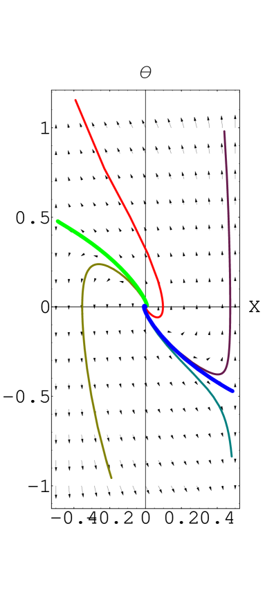
Figure 4: The phase space (for $m=n=2$). There is one interior equilibrium point at $(0,0)$ which represents the double cone. For $D<10$ it is focal repulsive but the spirals cannot be seen in the figure since their log-period is too large, while for $D\geq 10$ it is nodal repulsive, and hence the figure represents the whole range of dimensions. There are two finite equilibria on the boundary at $(1/m,\theta_{1})$ and $(-1/n,\theta_{2})$ which are saddle points. Each one has a critical curve which approaches it (heavy line). These two special trajectories denote the smoothed cones, where either ${\bf S}^{n}$ or ${\bf S}^{m}$ shrinks smoothly while the other one stays finite. Finally there are two attractive equilibria at infinity at $(1/m,-\infty)$ and $(-1/n,+\infty)$, and the thin lines trajectories represent generic trajectories which end at these infinite equilibrium points.

Linearized analysis of equilibrium points. The linearized dynamics around the an equilibrium point $(X_{q},\theta_{q})$ is given by the $2\times 2$ matrix $L$

$${d\over d\rho_{R}}\,\left[\begin{array}[]{c}\delta X\\ \delta\theta\end{array}\right]=L\left[\begin{array}[]{c}\delta X\\ \delta\theta\end{array}\right]~{},$$ (68)

where $\delta X:=X-X_{q},~{}\delta\theta:=\theta-\theta_{q}$. We remind the reader of the classification of equilibrium points

• If the eigenvalues of $L$ are complex (and necessarily self-conjugate since $L$ is real) then trajectories circle $(X_{q},\theta_{q})$ or spiral around it, and the point is called a focal point.

• If the eigenvalues of $L$ are real and of opposite sign then $(X_{q},\theta_{q})$ is called a saddle point and it is unstable in the sense that only if the initial conditions are fine-tuned to lie on a specific trajectory will the evolution flow into this point.

• If the eigenvalues of $L$ are real and of the same sign then $(X_{q},\theta_{q})$ is called a nodal point. If they are both positive then the point is called repulsive, while for negative it is called attractive. Naturally, the adjectives repulsive and attractive interchange under inversion of the flow (time reversal). A focal point may be called repulsive (or attractive) as well if the real parts of $L$’s eigenvalues are all positive (or negative).

For the double-cone $(X,\theta)=(0,0)$ we find

$$L_{0}=\left[\begin{array}[]{cc}0&~{}~{}~{}~{}-2/\sqrt{mn}\\ \sqrt{mn}&~{}~{}~{}~{}\sqrt{D-2}\end{array}\right]~{}.$$ (69)

The eigenvalues of this matrix are

$$\lambda_{\pm}={1\over 2}\,\left(\sqrt{D-2}\pm\sqrt{D-10}\right)$$ (70)

Let us make several observations

• The eigenvalues depend only on $D$ and not on $m,n$ separately.

• $D=10$ is a critical dimension, as found in [3].

  • For $D<10$ the eigenvalues are complex and we have a repulsive focal point.

  • For $D\geq 10$ the eigenvalues are real and we have a repulsive nodal point.

  • For the critical value $D=10$ the eigenvalues degenerate, but $L$ is not proportional to the identity matrix, but rather $L$ can be brought by a similarity transformation to the form

    $$\left[\begin{array}[]{cc}\sqrt{2}&~{}~{}1\\ 0&~{}~{}\sqrt{2}\end{array}\right]~{}.$$ (71)

• In the $D\to\infty$ limit we have $\lambda_{+}\simeq\sqrt{D},~{}\lambda_{-}\simeq 2/\sqrt{D}$.

• The eigenvectors which correspond to the eigenvalues $\lambda_{\pm}$ are $[2,~{}-\lambda_{\pm}\,\sqrt{mn}]$.

At the equilibrium point $(X_{1},\theta_{1})$ we find

$$L_{1}=\cosh{\theta_{1}}\,\left[\begin{array}[]{cc}{-2(D-1)\over m\sqrt{D-2}}&~{}~{}~{}~{}0\\ \sqrt{mn}&~{}~{}~{}~{}\sqrt{D-2}-{n\over m\sqrt{D-2}}\end{array}\right]~{}.$$ (72)

Similarly $L_{2}$ is obtained by substituting $\theta_{1}\leftrightarrow\theta_{2},~{}m\leftrightarrow n$. Since $\det{L}<0$ we see that at both $(1/m,\theta_{1})$ and $(-1/n,\theta_{2})$ we find a saddle point. The positive direction (eigenvector of the positive eigenvalue, defining the repulsive direction) is $[0,~{}1]$ in both cases, namely along the boundary.

Behavior at infinity. There are two attractive equilibrium points at infinity

$$\begin{array}[]{cc}X_{3}={1\over m{}{}}&~{}~{}\theta_{3}=-\infty\\ X_{4}=-{1\over n{}{}}&~{}~{}\theta_{4}=+\infty\end{array}~{}.$$ (73)

$(X_{3},\theta_{3})$ is attractive since for $\theta<\theta_{1}$ we have $dX/d\rho_{R}>0,~{}d\theta/d\rho_{R}<0$. There are no other fixed points at $\theta=-\infty$ but with $-1/n<X<1/m$ since $\lim_{\theta\to-\infty}dX/d\theta<0$. Moreover, close to $(X_{3},\theta_{3})$ the trajectories are found to asymptote exponentially fast to $X_{3}$, namely $|\delta X|\simeq\exp(-const\,\theta)$. Analogous properties hold for the attractive equilibrium point $(X_{4},\theta_{4})$.

The whole picture. Having found all the ingredients above we may assemble them into a complete phase diagram, figure 4, which is discussed in its caption.

The trajectories which end at $(X_{1},\theta_{1})$ and $(X_{2},\theta_{2})$ represent the smoothed cones. This is seen by transforming the definition of the smoothed cone through the changes of variables, as we proceed to explain. Before gauge fixing, one of the smoothed cones can be defined to behave in the limit $\rho\to 0$ as $B_{\rho}=0,~{}A\sim\log(\rho),~{}C\sim C_{0}$ (while for the other we interchange $A\leftrightarrow C$). After changing gauge and transforming to the $(X,P)$ variables this becomes $X_{1}=m/(m-1)\,\rho^{-2},~{}X_{2}=const\,\rho^{-2m/(m-1)},~{}P_{1}=-2/\rho,~{}P_{2}=-2m/(m-1)\,\rho^{-2}$ which in the $(X,\theta)$ variables tends to $(X_{1},\theta_{1})$ as defined in (67).

In summary, we have confirmed non-perturbatively the existence of the smoothed cones, going beyond the perturbative analysis of [3] near the smoothed tip. Altogether there is a one-parameter family of solutions which in the linear regime (far away from the tip) corresponds to the various linear combinations of the two linearized modes. Two of these solutions correspond to the smoothed cones, while all the rest end at infinity in phase space and yield a singular geometry. Even though strictly speaking our b.c. “$s_{+}$ prescription” is undefined for $l=0$ since $\Re(s_{1})=\Re(s_{2})$, we define it to mean to retain only the smoothed cone solutions, thereby the double-cone is an attractor at co-dim 1, as wanted, rather than at co-dim 2. Equivalently, these two special directions are defined up to multiplication by $\mathbb{R}_{+}$, and hence we loosely refer to them as a single mode which is normally defined up to multiplication by $\mathbb{R}$.

Acknowledgements

We would like to thank Ofer Aharony for a discussion. BK appreciates the hospitality of Amihay Hanany in MIT and KITP Santa Barbara where parts of this work were performed.

This research is supported in part by The Israel Science Foundation grant no 607/05 and by The Binational Science Foundation BSF-2004117.

Appendix A A numerical search for a DSS solution

In this section we present the details of our frustrated search for a Discretely Self-Similar (DSS) solution to the system, which if found, would have been a candidate to be the critical merger solution.

Formulation of the problem. The Lagrangian for the metric in the following form

$$ds^{2}=e^{2B_{\rho}(\rho,\chi)}d\rho^{2}+e^{2B_{\chi}(\rho,\chi)}\bigl{(}d\chi-f(\rho,\chi)d\rho\bigr{)}^{2}+e^{2\Phi(\rho,\chi)}dt^{2}+e^{2c(\rho,\chi)}d\Omega_{D-3}^{2}~{},$$ (74)

where $\rho$ here is the $\log$ of $\rho$ in (5), and choosing the gauge

$$f(\rho,\chi) = 0$$

$$B_{\rho}(\rho,\chi) = B_{\chi}(\rho,\chi)\equiv B(\rho,\chi)$$ (75)

is

$$L=-e^{\Psi}\bigl{[}2B^{\prime}\Psi^{\prime}+(D-3)C^{\prime}\bigl{(}\Psi^{\prime}+\Phi^{\prime}-C^{\prime}\bigr{)}+({}^{\prime}\rightarrow\dot{})\bigr{]}-\\ (D-3)(D-4)e^{\Psi+2B-2C},$$ (76)

where $\Psi=\Phi+(D-3)C$ as in (8) and prime and dot denote derivatives w.r.t $\rho$ and $\chi$. The constraints obtained from the gauge fixing (75) are

$$\dot{\Phi}^{\prime}+(D-3)\dot{C}^{\prime}+\Phi^{\prime}\dot{\Phi}+(D-3)C^{\prime}\dot{C}-(B^{\prime}\dot{\Phi}+\dot{B}\Phi^{\prime})-(D-3)(B^{\prime}\dot{C}+\dot{B}C^{\prime})=0,$$ (77)

$$\Phi^{\prime\prime}-\ddot{\Phi}+(D-3)(C^{\prime\prime}-\ddot{C})+\Phi^{\prime 2}-\dot{\Phi}^{2}+(D-3)(C^{\prime 2}-\dot{C}^{2})-\\ -2(B^{\prime}\Phi^{\prime}-\dot{B}\dot{\Phi})-2(D-3)(B^{\prime}C^{\prime}-\dot{B}\dot{C})=0,$$ (78)

and the equations of motion which follow from the Lagrangian are

$$\nabla^{2}B = -\frac{(D-3)(D-4)}{2}e^{2b-2c}+\frac{(D-3)(D-4)}{2}\bigl{(}C^{\prime 2}+\dot{C}^{2}\bigr{)}+(D-3)(C^{\prime}\Phi^{\prime}+\dot{C}\dot{\Phi})$$

$$\nabla^{2}\Phi = -(D-3)(C^{\prime}\Phi^{\prime}+\dot{C}\dot{\Phi})-\bigl{(}\Phi^{\prime 2}+\dot{\Phi}^{2}\bigr{)}$$

$$\nabla^{2}C = (D-4)e^{2b-2c}-(D-3)(C^{\prime 2}+\dot{C}^{2})-(C^{\prime}\Phi^{\prime}+\dot{C}\dot{\Phi})$$ (79)

where $\nabla^{2}$ is a 2-dimensional Laplacian $\nabla^{2}=\partial_{\rho\rho}+\partial_{\chi\chi}$.

We are looking for a Discretely Self-Similar (DSS) solution to these equations, one which satisfies $g_{\mu\nu}(\rho+\Delta_{\rho},\chi)=e^{2\Delta}g_{\mu\nu}(\rho,\chi)$ for some $\Delta$ and $\Delta_{\rho}$. In our equations we change $B\rightarrow B+\frac{\Delta}{\Delta_{\rho}}\rho$, $\Phi\rightarrow\Phi+\frac{\Delta}{\Delta_{\rho}}\rho$, $C\rightarrow C+\frac{\Delta}{\Delta_{\rho}}\rho$. The fields thus defined are periodic with period $\Delta_{\rho}$. Finally we make one more redefinition $\Phi\rightarrow\Phi+\ln{\cos{\chi/2}}$, influenced by the form of the double-cone solution (1). With the fields thus defined the double cone solution is constant

$$B(\rho,\chi) = \Phi(\rho,\chi)=-\frac{1}{2}\ln{\left(4(D-2)\right)}$$

$$C(\rho,\chi) = \frac{1}{2}\ln{\frac{D-4}{D-2}}~{}.$$ (80)

The boundary conditions which the fields should satisfy are

1. Reflection symmetry at the $\chi=0$ axis

   $$\dot{B}(\rho,0)=\dot{\Phi}(\rho,0)=\dot{C}(\rho,0)=0$$ (81)

2. Regularity at the horizon which is at $\chi=\pi$. There are 5 regularity conditions (3 from EOMs and 2 from constraints), but only 4 of them are independent. In terms of the newly defined fields these conditions read

   $$0=\dot{B}(\rho,\pi) = \dot{\Phi}(\rho,\pi)=\dot{C}(\rho,\pi)~{},$$

   $$B^{\prime}(\rho,\pi) = \Phi^{\prime}(\rho,\pi)~{}.$$ (82)

3. Periodicity in the $\rho$ direction as mentioned above

   $$0=\Phi(\rho+\Delta_{\rho})-\Phi(\rho)=B(\rho+\Delta_{\rho})-B(\rho)=C(\rho+\Delta_{\rho})-C(\rho)$$ (83)

Since our equations are invariant under the symmetry of adding 2 independent constants to the fields: $B\rightarrow B+const_{1}$, $C\rightarrow C+const_{1}$, $\Phi\rightarrow\Phi+const_{2}$, the last regularity condition can be integrated to the form $B(\rho,\pi)=\Phi(\rho,\pi)$ where setting the integration constant preserves only one remaining symmetry (scaling)

$$B\rightarrow B+const,C\rightarrow C+const,\Phi\rightarrow\Phi+const.$$ (84)

Algorithm. One way to find a DSS solution numerically is the following. Using the 5 equations that we have (3 elliptic and 2 hyperbolic) written as

$$f_{i}\bigl{(}B(\rho,\chi),\Phi(\rho,\chi),C(\rho,\chi),\Delta/\Delta_{\rho}\bigr{)}=0$$ (85)

with $i=1..5$, one constructs a “functional”

$$F_{0}[B(\rho,\chi),\Phi(\rho,\chi),C(\rho,\chi),\Delta,\Delta_{\rho}]:=\sum\limits_{i=1}^{5}\int\limits_{0}^{\pi}d\chi\int\limits_{0}^{\Delta_{\rho}}d\rho f_{i}^{2}\bigl{(}B(\rho,\chi),\Phi(\rho,\chi),C(\rho,\chi)\bigr{)}.$$ (86)

Note that in addition to the 3 (local) fields, the functional depends also on 2 global variables $\Delta$ and $\Delta_{\rho}$. This functional vanishes if it is evaluated on a solution and otherwise it is positive, so one can minimize it numerically. We are interested in a solution that satisfies our boundary conditions. Those in the $\chi$ direction (81,82) can be incorporated in the algorithm by defining one more non-negative functional:

$$F_{1}[B(\rho,\chi),\Phi(\rho,\chi),C(\rho,\chi)]:=\int\limits_{0}^{\Delta_{\rho}}d\rho\Bigl{[}\dot{B}^{2}(\rho,0)+\dot{\Phi}^{2}(\rho,0)+\dot{C}^{2}(\rho,0)\Bigr{]}+\\ +\int\limits_{0}^{\Delta_{\rho}}d\rho\Bigl{[}\dot{B}^{2}(\rho,\pi)+\dot{\Phi}^{2}(\rho,\pi)+\dot{C}^{2}(\rho,\pi)+(B(\rho,\pi)-\Phi(\rho,\pi))^{2}\Bigr{]}.$$ (87)

The boundary conditions in $\rho$ direction (83) is incorporated differently, as will be explained below.

The remaining symmetry (84) in the equations can be fixed in many possible ways; the most symmetric one being to set the overall average of the three fields to 0. It is done by the following functional:

$$F_{2}[B(\rho,\chi),\Phi(\rho,\chi),C(\rho,\chi)]:=\Bigl{[}\int\limits_{0}^{\pi}d\chi\int\limits_{0}^{\Delta_{\rho}}d\rho\Bigl{(}B(\rho,\chi)+\Phi(\rho,\chi)+C(\rho,\chi)\Bigr{)}\Bigr{]}^{2}.$$ (88)

The total functional to be minimized is

$$F:=F_{0}+F_{1}+F_{2}.$$ (89)

In order to prevent the procedure from converging to the double cone which is characterized by constant fields, we multiply $F$ by $\frac{1}{2}(v_{\rho}+\frac{1}{v_{\rho}})$ where the “variability” $v_{\rho}$ is defined by

$$v_{\rho}:=\int\limits_{0}^{\pi}d\chi\int\limits_{0}^{\Delta_{\rho}}d\rho\Bigl{(}B^{\prime 2}(\rho,\chi)+\Phi^{\prime 2}(\rho,\chi)+C^{\prime 2}(\rho,\chi)\Bigr{)}.$$ (90)

The $v_{\rho}$ term is added to prevent an endless drift towards an opposite limit, that of rapidly varying fields (since if $v_{\rho}\rightarrow\infty$ then $\frac{F}{v_{\rho}}$ would go to 0 no matter what happens to $F$) and a factor $\frac{1}{2}$ is added in order to fix the normalization since the value of the function $x+1/x$ at its minimum is 2.

The arbitrariness $\rho\rightarrow\rho+const$ is harmless, as will be explained below.

Discretization. By discretizing the domain $F$ becomes a function of a large number of (local) variables: $F=F(B_{ij},\Phi_{ij},C_{ij})$ where $B_{ij},\Phi_{ij},C_{ij}$ are the values of fields at the grid sites. We make the grid cells “non-square” as follows: if the step-size in $\chi$ direction is $h$ then we take the step-size in $\rho$ direction to be $h\cdot d$ with $d$ being adjustable parameter (in fact if the number of grid sites in both directions are equal then $d=\frac{\Delta_{\rho}}{\pi+h}$). In order to impose the boundary condition in the $\rho$ direction we calculate derivatives w.r.t. $\rho$ at the boundaries of the grid with values of fields at the opposite side of the grid, thus making our domain effectively cylindrical.

One can start with some configuration of fields and change them together with the global variables $\Delta$ and $\Delta_{\rho}$ so that $F$ is minimized (remembering that only $F=0$ minima are solutions). This is done by calculating the gradient $\partial F/\partial B_{ij}$, $\partial F/\partial\Phi_{ij}$, $\partial F/\partial C_{ij}$, $\partial F/\partial\Delta$, $\partial F/\partial\Delta_{\rho}$ (the direction in a “space of parameters” in which $F$ grows in the fastest way) and going a bit in the opposite direction. This procedure is repeated until we arrive at a minimum. There is an additional parameter $\Omega$ which sets the “speed of relaxation” by defining the change in any parameter $a$ to be $a\rightarrow a-\Omega\,\frac{\partial F}{\partial a}$. Instead of working with the global variables $\Delta$ and $\Delta_{\rho}$ we find it convenient to use the equivalent variables $d$ and $\delta=\frac{\Delta}{\Delta_{\rho}}$. Finally, the symmetry $\rho\rightarrow\rho+const$ is of no importance because nothing in the algorithm produces running in this direction. Moreover, discretization makes this symmetry discrete and creates a finite distance between nearby degenerate vacua.

Results. We ran a program with $D=5$, and so far the only solution found is the double cone, even after using various “tricks” designed to avoid it, as described below. If multiplication by $\frac{1}{2}(v_{\rho}+\frac{1}{v_{\rho}})$ is not used the program converges to the double cone very fast no matter what the initial configuration is. If this factor is included then it still converges to this solution with $d\rightarrow\infty$. If one adds to $F$ an additional factor $\frac{1}{2}(d+\frac{1}{d})$ then it still converges to the double cone but in a much longer time, so that $F$ tends to 0 faster than $1/v_{\rho}$ tends to infinity (the configuration becomes very sensitive to changes, so it is necessary to take $\Omega$ very small, for a grid 10$\times$10 it should be of order $10^{-6}$ whereas without this additional factor it works well with $\Omega\approx 10^{-3}$). In all cases $\delta$ becomes close to that of the double cone solution $\frac{1}{2\sqrt{3}}\approx 0.2887$.

References

- [1] B. Kol, “The phase transition between caged black holes and black strings: A review,” Phys. Rept. 422, 119 (2006) [arXiv:hep-th/0411240].
- [2] T. Harmark and N. A. Obers, “Phases of Kaluza-Klein black holes: A brief review,” arXiv:hep-th/0503020.
- [3] B. Kol, “Topology change in general relativity and the black-hole black-string transition,” JHEP 0510, 049 (2005) [arXiv:hep-th/0206220].
- [4] T. Wiseman, “Static axisymmetric vacuum solutions and non-uniform black strings,” Class. Quant. Grav. 20, 1137 (2003) [arXiv:hep-th/0209051].
- [5] E. Sorkin, B. Kol and T. Piran, “Caged black holes: Black holes in compactified spacetimes. II: 5d numerical implementation,” Phys. Rev. D 69, 064032 (2004) [arXiv:hep-th/0310096].
- [6] H. Kudoh and T. Wiseman, “Properties of Kaluza-Klein black holes,” Prog. Theor. Phys. 111, 475 (2004) [arXiv:hep-th/0310104].
- [7] H. Kudoh and T. Wiseman, “Connecting black holes and black strings,” Phys. Rev. Lett. 94, 161102 (2005) [arXiv:hep-th/0409111].
- [8] B. Kleihaus, J. Kunz and E. Radu, “New nonuniform black string solutions,” JHEP 0606, 016 (2006) [arXiv:hep-th/0603119].
- [9] B. Kol, “Choptuik scaling and the merger transition,” arXiv:hep-th/0502033.
- [10] M. W. Choptuik, “Universality and scaling in gravitational collapse of a massless scalar field,” Phys. Rev. Lett. 70, 9 (1993).
- [11] C. Gundlach, “Critical phenomena in gravitational collapse,” Phys. Rept. 376, 339 (2003) [arXiv:gr-qc/0210101].
- [12] B. Kol and T. Wiseman, “Evidence that highly non-uniform black strings have a conical waist,” Class. Quant. Grav. 20, 3493 (2003) [arXiv:hep-th/0304070].
- [13] E. Sorkin and Y. Oren, “On Choptuik’s scaling in higher dimensions,” Phys. Rev. D 71, 124005 (2005) [arXiv:hep-th/0502034].
- [14] C. Gundlach, “Understanding critical collapse of a scalar field,” Phys. Rev. D 55, 695 (1997) [arXiv:gr-qc/9604019].
- [15] S. Hod and T. Piran, “Fine-structure of Choptuik’s mass-scaling relation,” Phys. Rev. D 55, 440 (1997) [arXiv:gr-qc/9606087].
- [16] C. Gundlach, “The Choptuik space-time as an eigenvalue problem,” Phys. Rev. Lett. 75, 3214 (1995) [arXiv:gr-qc/9507054].
- [17] V. P. Frolov, A. L. Larsen and M. Christensen, “Domain wall interacting with a black hole: A new example of critical phenomena,” Phys. Rev. D 59, 125008 (1999) [arXiv:hep-th/9811148].
- [18] V. P. Frolov, “Merger transitions in brane-black-hole systems: Criticality, scaling, and self-similarity,” arXiv:gr-qc/0604114.
- [19] G. K. Savvidy, “Yang-Mills Classical Mechanics As A Kolmogorov K System,” Phys. Lett. B 130, 303 (1983).