Search of a general form of superpotential in hierarchy with discrete energy spectrum

Abstract

In paper a generalized definition of superpotential has proposed, which connects two one-dimensional potentials $V_{1}$ and $V_{2}$ with discrete energy spectra completely and where:

• for definition of an energy of factorization an arbitrary level of the energy spectrum of the given $V_{1}$ is used and a function of factorization is defined concerning a bound (ground or excited) state at this energy level,

• for the definition of the energy of factorization an arbitrary energy (which can be not coincident with levels of the spectrum of $V_{1}$) is used and the function of factorization is defined concerning an unbound (or non-normalizable) state at this energy.

It has shown, that for the unknown superpotential such its definition follows directly from a solution of Riccati equation at the given potential $V_{1}$.

Using the arbitrary bound state in the construction of the superpotential, the SUSY QM methods at their effectiveness in construction of new exactly solvable potentials on the basis of the given potential $V_{1}$, in detail calculations of spectral characteristics under the deformation of $V_{1}$ have been coming to a level of methods of inverse problem. So, if as the given potential $V_{1}$ to choose a rectangular well with finite width and infinitely high walls, then we reconstruct by SUSY QM approach all pictures of deformation (without displacement of the levels in the spectrum) of this potential and its wave functions of the lowest bound states, which were obtained early by the methods of the inverse problem. Here, interdependence between parameters of the deformation for the methods of SUSY QM and the inverse problem has found, an analysis of a behavior of wave functions and the potential under the deformation has fulfilled, a classification has proposed for zero-points of the potential, nodes of the deformed wave functions, points, where wave functions are not deformed, an analysis of angles of wave functions leaving from such points has fulfilled.

Using the unbound and non-normalizable states at the arbitrary energy of factorization in the definition of the superpotential, we obtain new types of deformations. So, using only one superpotential, one can join two potentials, which have the real energy spectra with own bound states and without coincident levels.

PACS numbers: 11.30.Pb, 03.65.-w, 12.60.Jv, 03.65.Xp, 03.65.Fd

Keywords: supersymmetric quantum mechanics, exactly solvable models, Riccati equation, Darboux transformations, method of factorization, unbound and non-normalizable states in discrete spectrum, $n$-parametric family of isospectral potentials, rectangular well.

Designations

In paper we shall use the following designations.

• The first potential $V_{1}$, on the basis of which we construct new potentials using SUSY-transformations, we shall name as the starting potential with number “1”.

• $\varphi_{i}^{(k)}$ is wave function (WF or WFs — in the plural case, partial or general solution) of the potential $V_{k}$ with the number $k$, where instead of index $i$ at the bottom we shall use one index from the following:

  • $n$ — as the number of the level of discrete energy spectrum of the potential $V_{k}$ with number $k$, if this level does not coincide with energy of factorization $\cal E$ (i. e. the energy, at which the superpotential is defined);

  • $m$ — as the number of the level of the discrete energy spectrum of the potential $V_{k}$ with the number $k$, if this level coincides with the energy of factorization $\cal E$;

  • $w$ — as the index at energy, which coincides with the energy of factorization $\cal E$ and does not coincide with any level of the energy spectrum of the starting potential $V_{1}$.

• $E_{i}^{(k)}$ is the level with the number $i$ (corresponding to WF $\varphi_{i}^{(k)}$) of the energy spectrum for the potential $V_{k}$. We shall number the levels of the discrete spectrum so:

  • the lowest level, concerned with the ground bound state, by number “1”;

  • the next levels, located higher and described excited bound states, by numbers “2” and so on.

• $W_{i}^{(k)}$ is the superpotential, for which as the energy of factorization we shall choose the energy with index $i$, and as a function of factorization we shall choose WF $\varphi_{i}^{(k)}$ (of bound or unbound state) of the potential $V_{k}$. If the function $W_{i}^{(k)}$ will be considered with only one number $k$ in the text, then we omit this number sometimes.

• We shall choose such definition of operators $A_{i}$ and $A_{i}^{+}$:

  $$\begin{array}[]{cc}A_{i}=\displaystyle\frac{d}{dx}+W_{i}(x),&A_{i}^{+}=-\displaystyle\frac{d}{dx}+W_{i}(x).\end{array}$$ (1)

• $\bar{\varphi_{i}}^{(k)}$ is WF of unbound or non-normalizable state, which we shall denote by stroke on top.

1 Introduction

Supersymmetric theories are ones from the most modern and vigorously developed topics of physics of particles and interactions. Usually, under a word “supersymmetry” we have in mind a relation established between bosons and fermions, which allows to consider the boson and the fermion as two different manifestations of an unified particle [1]. It is interesting to note, that according to one of main principles of quantum mechanics (without applying a formalism of field theories), a conception of “wave” (which we relate to interactions in the simplest understanding) and a conception of “particle” (under which we keep in mind the matter in the simplest understanding) can be considered as two different manifestations of only one object — “particle-wave”. Mathematically, for description of the particles and interactions the supersymmetric models (for example, such as Minimal Supersymmetric Standard Model [2, 3]), based on a modern apparatus of quantum field theory mainly with application of algebras of supersymmetry [4], are used. It makes study of properties of interdependence between fields of the matter (as the fermion fields) and fields of the interactions (as the boson fields) enough complicated.

In 1981 E. Witten in his famous paper [5] constructed a simple example of one-dimensional supersymmetric system, which has no any reference to the theory of fields at all! It had opened a possibility to study absolutely independently properties of supersymmetric transformations between partners on the basis of the simplest examples, without using formalism of the field theories (and without formalism for description of spin). Since then, after publishing of some fundamental papers, a new topic of physics had been created and has been developed vigorously, which is named as supersymmetric quantum mechanics (SUSY QM) [6].

An essential interest in SUSY QM can be explained by that it allows to study in details the properties of the supersymmetric transformations, using the simplest quantum systems. Of cause, then such results can be applied in the field theories up to cosmology [7] and quantum gravity. So, in the paper [8] (see p. 2917–2918) C. V. Sukumar clearly explained such connection so (also see [9, 10] of other authors): “It is well known that $d=1$ quantum mechanics is formally equivalent to the $d=1$ quantum field theory with the identification $x\to\varphi$, $p\to\partial_{t}\varphi$ and canonical quantisation of the field $\varphi$ leads to the usual commutation relation between $x$ and $p$ …”

From another side, the second important perspective of SUSY QM has been opened: it improves essentially methods of quantum mechanics directly. Keeping in the frameworks of quantum mechanics, SUSY QM proposes to researcher its own simple mathematically and clear enough methods for calculation of spectral characteristics of quantum systems, it gives answers to questions and vagueness, putted early by methods of direct and inverse problems of quantum mechanics. First of all, one note a method of factorization (principally, introduced at the first time by A. A. Andrianov, N. V. Borisov and M. V. Ioffe in [11] and independently by C. V. Sukumar at first in [12] and then in [8, 13, 14, 15, 16, 17] where a main formalism of such a method was constructed, however, the algorithm of factorization, started else by P. A. M. Dirac in [18] and E. Schrödinger in [19], can be found earlier for solution of the spectral problem with some simplest one-dimensional potentials in quantum mechanics, for example, see [20, 21]), formulation of which has been causing a large number of papers in SUSY QM, search of new methods and opening of new types of exactly solvable potentials on the basis of intensive study of Darboux transformations (first of all, one can point out papers of B. F. Samsonov, V. G. Bagrov with their colleagues at development of a general formalism of these transformations with their application in a number of different problems [22, 23, 24, 25, 26], it is necessary to note papers of other researchers at their investigations of these transformations with application to theory of solitons [27, 28, 29], in approaches of nonlinear supersymmetry [30, 31, 32], in solution of matrix Schrödinger equations [33], in solution of system of coupled discrete Schrödinger equations [34], in generalization of the formalism of these transformations for three-dimensional and many-dimensional spaces [11, 35, 36, 37], in scattering theory [38, 23, 25], in improvement of the methods of the inverse problem on the basis of these transformations [39], in study of interdependence between these transformations, the method of factorization and the methods of the inverse problem [35, 40, 41], in intriguing and having large perspectives non-stationary approaches [42, 43], one can note approach of the inverse Darboux transformations in description of some types of exactly solvable potentials [44], and also interesting review about such Darboux transformations [45] and historical paper [46]).

An essential progress was achieved early in development of the methods of the inverse problem in construction of the new exactly solvable potentials on the basis of known ones (see [47, 48, 49]). A vigorous accumulation of information about new types of the potentials with spectral characteristics, which have explicit analytical form, little by little forms an unified theory of exactly solvable models (or potentials) (see [47], p. 915). The methods of SUSY QM, after their opening of original solutions for new types of such potentials (for example, shape invariant potentials or SIP-potentials [50, 6] with translations of parameters [51, 52, 53], with scaling of the parameters [54, 55], with rotations of parameters [56], class of the potentials of Shabat and Spiridonov [57, 58, 51], which includes soliton-like reflectionless solutions without tunneling, search of the reflectionless potentials with barriers [59, 60, 61] (where an effect of reflectionless tunneling can appear, existence of which is discussed up to now), the potentials in approach of nonlinear supersymmetry [31, 32]), have proved their right to originality, and their effectiveness in detail calculations of spectral characteristics of the potentials comes little by little to a level of the methods of the inverse problem. During last two decades, one can see a continuous competition between the methods of the inverse problem and SUSY QM methods, which supplement each other [13, 15, 17]. However, perhaps, increase of number of the new SUSY QM methods looks more intensive, that one can explain by their comparative simplicity and availability.

These arguments emphasize the interest in the further development of the new SUSY QM methods, which give to researcher the enlarger possibilities in construction of the new exactly solvable potentials (on the basis of known potentials) in comparison with early known methods.

In this paper we shall restrict ourselves by consideration of one-dimensional potentials with discrete spectra of energy completely. Here, we shall analyze more generalized definition of a superpotential, which we construct in the region of real values only and which connects two potentials SUSY-partners in frameworks of the most widely known approach of SUSY QM (for example, as in formalism [8, 6]), adding an arbitrariness into a choice of a bound state at an energy of factorization, which coincides with the ground or excited level of the energy spectrum of the given potential $V_{1}$, and introducing an arbitrary unbound and non-normalizable states at the arbitrary energy of factorization, which can be not coincident with the levels of the energy spectrum of $V_{1}$. We note, that similar generalizations on the construction of the superpotential were considered early (see [15] — more for the potentials with continuous energy spectra; [62] p. 378–386 — for the superpotential and the energy of factorization in the region of complex values). However, we see, that this question for the potentials with discrete energy spectra has not been studied yet practically, and our analysis has shown an extreme availability of taking into account of different types of states at the arbitrary energy of factorization in the definition of the superpotential, even if to find it in the region of real values only.

It turns out, that such generalization follows directly from a form of the superpotential, if to find it as an exact solution of Riccati equation at a given potential $V_{1}$, own independent variant of which we present in Sec. 2 (see also original papers [8, 63, 64, 65, 66, 67, 68, 69, 70, 71, 72] and monographs [73, 74]). It is necessary to note, that the Riccati equation admits an arbitrariness in a choice of boundary conditions in the definition of the superpotential, while the standard approach to the construction of the superpotential uses wave function of the bound (mainly, ground) state only and, therefore, it is partial.

The generalization for definition of the superpotential requires introduction of the unbound or non-normalizable states at the arbitrary energy of factorization, and a formalism of such states we present in Sec. 4 (also see [8] p. 2925–2934, [6] p. 324–325, [49] p. 286–290, 293–297, 309–318, [62] p. 378–382, 382–389). In Sec. 5 we improve a method of construction of $n$-parametric family of isospectral potentials, developed early in [6] (see p. 326–328).

Generalizing the definition of the superpotential on the basis of wave function of the arbitrary excited bound state of the given potential $V_{1}$, we have achieved practically full analogous between SUSY QM methods and the methods of the inverse problem. So, in Sec. 6 we reconstruct all pictures of the deformation (without of displacement of the levels) of a rectangular well with finite width and infinitely high walls and its wave functions of the lowest bound states, which were obtained early in the review [47] (see p. 916–919) on the basis of the methods of the inverse problem. Here, we find interdependence between main parameters of deformation for the SUSY QM methods and the methods of the inverse problem, find answers (confirmed by analytical expressions) on some questions, putted early in this review. These arguments make the SUSY QM methods practically such effective as the methods of the inverse problem.

We see, that use of the unbound states in the definition of the superpotential (in the energy region of the real values) opens new original perspectives for the SUSY QM methods. It turns out, that if to do not restrict oneself by the bound states only in the definition of the superpotential, but to construct it on the basis of a function, which is a general (or partial) solution (without implying the boundary conditions for bound states on it) of the Schrödinger equation with the starting potential $V_{1}$ at the arbitrary energy (which can be not coincident with the energy levels of $V_{1}$), then we obtain new exactly solvable potentials which have own energy spectra with the bound states. In particular, using only one superpotential, one can join two potentials, energy spectra of which (with own bound states) have no one coincident level (it has found at the first time in the supersymmetric approach)! As a demonstration, in Sec. 7 we present two new approaches of construction of the new potentials, where as the starting potential $V_{1}$ we use the rectangular well with infinitely high external walls. This opens a possibility to deform at once whole energy spectrum for the given potential (perhaps, by a given rule, for example, as for SIP-potentials with scaling of the parameters). Perhaps, such a way will open a possibility to connect together boson and fermion components with absolutely different energy spectra in the supersymmetric quantum theory of fields, using only one superpotential.

2 An exact analytical solution of a superpotential at the given potential

To clarify, which the most general form an unknown superpotential can have, when we know only a form of the potential, concerning with this superpotential in the most prevailing formalism (for example, as in [6] p. 275–277, [8] p. 2922-2923, 2925–2927, [11] p. 19–20, at an energy of factorization, located not higher then the lowest level of energy spectrum of the given potential), we inevitably come to a problem of a solution of Riccati equation, where as unknown function the superpotential is used.

2.1 The superpotential as the solution of the Riccati equation

Let’s consider a quantum system with a potential $V_{1}(x)$ and a discrete energy spectrum completely. For such a system one can write down the Schrödinger equation:

$$\begin{array}[]{ccl}\hat{h}_{1}\varphi^{(1)}_{m}(x)&=&\biggl{(}-\displaystyle\frac{d^{2}}{dx^{2}}+V_{1}(x)\biggr{)}\varphi^{(1)}_{m}(x)=E^{(1)}_{m}\varphi^{(1)}_{m}(x),\end{array}$$ (2)

where $\hat{h}_{1}$ is Hamiltonian of the system, $\varphi^{(1)}_{m}(x)$ is wave function (WF) of a state with a number $m$ of this system, $E_{m}^{(1)}$ is energy level, corresponding to the state with the number $m$, $E_{1}^{(1)}$ is the lowest level of the energy spectrum with the number $1$. For the given potential one can introduce a superpotential $W(x)$, defining it by such a condition (for example, according to [6], p. 287–289):

$$V_{1}(x)=W^{2}(x)-\displaystyle\frac{dW(x)}{dx}+E^{(1)}_{1}.$$ (3)

Let the potential $V_{1}(x)$ be exactly solvable, i. e. one can write WFs for all states and the energy spectrum of the system with such a potential in the explicit analytical form. Let’s assume, that we know a form of the potential $V_{1}(x)$, its WFs and the energy spectrum. Also we assume, that we do not know the superpotential $W(x)$ and we shall find it. The condition (3), defining the unknown superpotential $W(x)$, is the Riccati equation (see in the Introduction citations on some original papers and monographs). Let’s find the form of the superpotential, solving this equation.

We fulfill a substitution of variable $x\to u=u(x)$, defining it so:

$$f(x)=\displaystyle\frac{du(x)}{dx},$$ (4)

where on the function $f(x)$ we impose arbitrariness in its choice. We obtain:

$$\begin{array}[]{ll}du(x)=fdx,&\displaystyle\frac{d}{dx}=f\displaystyle\frac{d}{du}.\end{array}$$ (5)

Then one can rewrite the equation (3) through new variables:

$$V_{1}(u)-E^{(1)}_{1}=W^{2}(u)-f(u)\displaystyle\frac{dW(u)}{du}.$$ (6)

Now let’s consider a function of a from:

$$\begin{array}[]{l}W_{R}(u)=\left\{\begin{array}[]{cl}-\displaystyle\frac{\alpha}{u-u_{0}},&\mbox{at }u\leq 0,\\ -\displaystyle\frac{\alpha}{u+u_{0}},&\mbox{at }u\geq 0,\end{array}\right.\end{array}$$ (7)

where $\alpha>0$ and $u_{0}>0$ are constant real parameters. By direct substitution one can make sure, that at $\alpha=1$ the potential

$$V_{R}(u)=W_{R}^{2}(u)-\displaystyle\frac{dW_{R}(u)}{du}$$ (8)

becomes zero (according to [59, 60], the function of the form (7) is only one from five possible solutions for the superpotential $W_{R}$, on the basis of which one can construct zero potential (8); therefore, the choice (7) further will give us only a partial solution in the definition of the superpotential $W(x)$; therefore, for example, substitutions (A3) and $y=1/\varphi$ in [8], perhaps, lead to the partial definition of the superpotential $U$ in the form (A12) at the energy of factorization $E$ located not higher then the lowest level of the energy spectrum of the potential $V$). In the definition of the function $W_{R}(u)$ in the form (7) its divergence at point $u=0$ is excluded by introduction of the non-zero parameter $u_{0}$; however, the function $W_{R}(u)$ has discontinuity at zero, nevertheless constructed on its basis the function $V_{R}(u)$ is continuous at this point, and, therefore, on all axis $u$ (for example, in contrast to the function $y(x)$ in limit $\varphi(x)\to 0$ at substitution $y=1/\varphi$ in [8], p. 2934; exclusion of such a divergence for the function $y(x)$ and/or $\varphi(x)$ at passing of the variable $x$ through the extreme value $x=0$ can be interesting, because it allows to consider oscillations of the functions $y(x)$ and $\varphi(x)$; it is important to study a question of passing of these functions through their zero values or “nodes”, nevertheless it turns out, that it is possible to define the superpotential at the energy of factorization, which coincides not only with the lowest level of the energy spectrum for the given potential or below it, but and higher then such level). Here, in future investigations, it is interesting to use a formalism for obtaining solutions for “the regulized one-dimensional form of the centrifugal potential $V(x)=\alpha/(x+i\epsilon)^{2}$” where $\alpha$ is a real strength and $\epsilon$ a real constant that removes the singularity at the origin, proposed in [75] (see p. 32–34), as a possible further complex extensions of a definition of the function $W_{R}(u)$ in search of new types of exact solutions of Riccati equation by the approach proposed in this section.

For simplicity of analysis further we shall consider the function $V_{R}(u)$ on the positive semi-axis $u>0$. Subtracting this function from the expression (6), we obtain:

$$V_{1}(u)-E^{(1)}_{1}=W^{2}(u)-f(u)\displaystyle\frac{dW(u)}{du}-f^{2}(u)\biggl{(}W_{R}^{2}(u)-\displaystyle\frac{dW_{R}(u)}{du}\biggr{)},$$ (9)

here multiplication of $V_{R}(u)$ on square of the function $f(u)$ leaves this function as zero.

Now fix $f(u)$ by such a condition:

$$f(u)W_{R}(u)=W(x).$$ (10)

Then from (9) we find:

$$\begin{array}[]{c}V_{1}(x)-E^{(1)}_{1}=f^{2}(u)W_{R}^{2}(u)-f(u)\displaystyle\frac{dW(u)}{du}-f^{2}(u)W_{R}^{2}(u)+f^{2}(u)\displaystyle\frac{dW_{R}(u)}{du}=\\ =-f(u)\displaystyle\frac{d}{du}\biggl{(}f(u)W_{R}(u)\biggr{)}+f^{2}(u)\displaystyle\frac{dW_{R}(u)}{du}=\par-f(u)\displaystyle\frac{df(u)}{du}W_{R}(u)-\\ -f^{2}(u)\displaystyle\frac{dW_{R}(u)}{du}+f^{2}(u)\displaystyle\frac{dW_{R}(u)}{du}=\par-\displaystyle\frac{1}{2}\displaystyle\frac{df^{2}(u)}{du}W_{R}(u).\end{array}$$ (11)

From here we find $f(u)$:

$$\frac{df^{2}(u)}{du}=\displaystyle\frac{2\Bigl{(}E^{(1)}_{1}-V_{1}(x)\Bigr{)}}{W_{R}(u)}.$$ (12)

Thus, we have found the function $f(u)$ in dependence on the known potential $V_{1}(x)$ and the superpotential $W_{R}(u)$. However, it is failed to integrate explicitly this expression else, because implicit dependence of the function $W_{R}(u)$ on the variable $f$ is included into the right part of (12), and $V_{1}(x)$ depends on $x$.

Taking into account (5), we rewrite (12) by such a way:

$$\begin{array}[]{ll}W_{R}(u)\displaystyle\frac{df^{2}(u)}{du}=2W_{R}(u)f(u)\displaystyle\frac{d}{du}f(u)=2W_{R}(u)\displaystyle\frac{df(u)}{dx}=2\Bigl{(}E^{(1)}_{1}-V_{1}(x)\Bigr{)}.\end{array}$$

$$W_{R}(u)\displaystyle\frac{df(u)}{dx}=E^{(1)}_{1}-V_{1}(x).$$ (13)

We have obtained the equation, in which the left and right parts depend only on one variable $u$ or $x$. Further, using the solution (7) for non-zero superpotential $W_{R}$ (at $u>0$), we obtain:

$$\begin{array}[]{ll}-\displaystyle\frac{\alpha}{u+u_{0}}\displaystyle\frac{df(u)}{dx}=-\displaystyle\frac{\alpha}{u+u_{0}}\displaystyle\frac{d}{dx}\displaystyle\frac{du(x)}{dx}=-\displaystyle\frac{\alpha}{u+u_{0}}\displaystyle\frac{d^{2}u(x)}{dx^{2}}=E^{(1)}_{1}-V_{1}(x)\end{array}$$

or (at $\alpha=1$)

$$\biggl{(}-\displaystyle\frac{d^{2}}{dx^{2}}+V_{1}(x)\biggr{)}\Bigl{(}u(x)+u_{0}\Bigr{)}=E^{(1)}_{1}\Bigl{(}u(x)+u_{0}\Bigr{)}.$$ (14)

Thus, we have obtained the Schrödinger equation for the potential $V_{1}(x)$!

Solving the Schrödinger equation at selected energy, one can find a general form of the function $u(x)+u_{0}$. Usually, for potentials with infinitely high external walls the bound states cause a physical interest, WFs of which tend to zero in asymptotic space regions. Such boundary condition, imposed on WFs, introduces restrictions on possible energy values, defining the discrete spectrum.

The level $E^{(1)}_{1}$ is the lowest level of the energy spectrum for the potential $V_{1}(x)$. Therefore, this level is eigenvalue of the Hamiltonian $\hat{H}^{(1)}$, for which there is non-zero solution for the function $u(x)+u_{0}$, being the WF. According to set of the problem, the value $E^{(1)}_{1}$ and WF concerned with it are known to us. One can write:

$$\begin{array}[]{ccl}u(x)&=&C_{0}\varphi^{(1)}_{1}(x)-u_{0},\\ f(x)&=&\displaystyle\frac{du(x)}{dx}=C_{0}\displaystyle\frac{d\varphi^{(1)}_{1}(x)}{dx},\\ W_{R}(x)&=&-\displaystyle\frac{1}{u(x)+u_{0}}=-\displaystyle\frac{1}{C_{0}\varphi^{(1)}_{1}(x)},\\ W(x)&=&f(x)W_{R}(u(x))=-\displaystyle\frac{1}{\varphi^{(1)}_{1}(x)}\displaystyle\frac{d\varphi^{(1)}_{1}(x)}{dx}=-\displaystyle\frac{d}{dx}\log\Bigl{(}\varphi^{(1)}_{1}(x)\Bigr{)},\\ C_{0}&=&const.\end{array}$$ (15)

Note, that the found solution for the superpotential $W_{n}(x)$ has obtained only in such interval of values $x$, where $u(x)>0$ ($u(x)$ is the continuous function in this interval), and therefore such a determination of the superpotential does not contain divergences. It agrees with a behavior of WF of the bound state at the lowest energy level, which has no nodes.

One can define a form of a potential-partner $V_{2}(x)$ so:

$$V_{2}(x)=W^{2}(x)+\displaystyle\frac{dW^{2}(x)}{dx}+E^{(1)}_{1}.$$ (16)

Usually, if the superpotential $W(w)$ is defined in the form of fourth expression from (15), then the energy level $E^{(1)}_{1}$ is named as an energy of factorization (let’s denote it as $\cal E$), and the function $\varphi^{(1)}_{1}(x)$, defining the superpotential by such a way, is named as a function of factorization.

Conclusion:

The solution for the superpotential was obtained by resolving the Riccati equation. In obtaining of the equation (14) for determination of the superpotential we do not use the boundary conditions, which can be imposed on the function $u(x)$. Further, applying the boundary conditions, we define a state, described by the function $u(x)$, as bound one at the energy of factorization, coincident with the lowest energy level $E^{(1)}_{1}$. Therefore, the solution (15), constructed on the basis of WF of the bound state at the energy of factorization, coincident with the lowest level $E^{(1)}_{1}$, can be a partial solution in definition of the superpotential $W(x)$.

2.2 Arbitrariness in a choice of the energy of factorization

Now let’s assume, that for considered above quantum system with the potential $V_{1}(x)$ one can define the superpotential $W(x)$ instead of the condition (3) by the following:

$$V_{1}(x)=W^{2}(x)-\displaystyle\frac{dW(x)}{dx}+E^{(1)}_{1}+\Delta E^{(1)},$$ (17)

where $\Delta E^{(1)}$ is arbitrary real number.

Assuming WF and energy spectrum for the potential $V_{1}$ as known to us, we find the superpotential in this case. Then in the approach, presented in the previous section, we obtain instead of (14) the following equation:

$$\biggl{(}-\displaystyle\frac{d^{2}}{dx^{2}}+V_{1}(x)\biggr{)}\Bigl{(}u(x)+u_{0}\Bigr{)}=\Bigl{(}E^{(1)}_{1}+\Delta E^{(1)}\Bigr{)}\Bigl{(}u(x)+u_{0}\Bigr{)}.$$ (18)

We again obtain the Schrödinger equation with the potential $V_{1}(x)$. From (18) we find:

• If the energy $E^{(1)}_{1}+\Delta E^{(1)}$ coincides with arbitrary level $E^{(1)}_{m}$ with a number $m$ of the energy spectrum for the potential $V_{1}$, then it is eigenvalue of the Hamiltonian $\hat{H}^{(1)}$, for which there is non-zero solution $u(x)+u_{0}$ of the equation (18), described a bound state for $V_{1}$ at the selected value $\Delta E^{(1)}$. Then the solution for the superpotential $W(x)$ exists, where $E^{(1)}_{1}+\Delta E^{(1)}$ is the energy of factorization:

  $$\begin{array}[]{ccl}u(x)&=&C_{m}\varphi^{(1)}_{m}(x)-u_{0},\\ f(x)&=&\displaystyle\frac{du(x)}{dx}=C_{m}\displaystyle\frac{d\varphi^{(1)}_{m}(x)}{dx},\\ W_{R}(x)&=&-\displaystyle\frac{1}{u(x)+u_{0}}=-\displaystyle\frac{1}{C_{m}\varphi^{(1)}_{m}(x)},\\ W(x)&=&f(x)W_{R}(u(x))=-\displaystyle\frac{1}{\varphi^{(1)}_{m}(x)}\displaystyle\frac{d\varphi^{(1)}_{m}(x)}{dx}=-\displaystyle\frac{d}{dx}\log{\bigl{|}\varphi^{(1)}_{m}(x)\bigr{|}},\\ C_{m}&=&const.\end{array}$$ (19)

• If the value $E^{(1)}_{1}+\Delta E^{(1)}$ does not coincide with any level $E^{(1)}_{m}$ from the energy spectrum of the potential $V_{1}$, then it cannot be eigenvalue of the Hamiltonian $\hat{h}_{1}$ and, therefore, there is no any non-zero solution $u(x)+u_{0}$ of the equation (18), described the bound state for $V_{1}$ at the selected value $\Delta E^{(1)}$ (with interdependence (17) between the potential $V_{1}(x)$ and the superpotential $W(x)$).

• Each separate known solution for wave function with its level of the energy spectrum of the potential $V_{1}$ gives a new independent solution for the superpotential $W(x)$, and concerned with it the energy of factorization.

However, so defined superpotential can have divergent values at points-nodes of WFs of exited bound states for $V_{1}$, it turns out, that by use of it one can construct new exactly solvable potentials with bound states and without divergences. Therefore, further in this paper we shall suppose a possibility of definition of the superpotential with divergences at isolated points.

2.3 An exact solution for the superpotential with next number in the hierarchy

Let’s consider three Hamiltonians $\hat{h}_{n}$, $\hat{h}_{n+1}$ and $\hat{h}_{n+2}$ for three potentials $V_{n}(x)$, $V_{n+1}(x)$ and $V_{n+2}(x)$ with discrete energy spectra completely:

$$\begin{array}[]{lclcl}\hat{h}_{n}\varphi^{(n)}_{l}(x)&=&\biggl{(}-\displaystyle\frac{d^{2}}{dx^{2}}+V_{n}(x)\biggr{)}\varphi^{(n)}_{l}(x)&=&E^{(n)}_{l}\varphi^{(n)}_{l}(x),\\ \hat{h}_{n+1}\varphi^{(n+1)}_{m}(x)&=&\biggl{(}-\displaystyle\frac{d^{2}}{dx^{2}}+V_{n+1}(x)\biggr{)}\varphi^{(n+1)}_{m}(x)&=&E^{(n+1)}_{m}\varphi^{(n+1)}_{m}(x),\\ \hat{h}_{n+2}\varphi^{(n+2)}_{k}(x)&=&\biggl{(}-\displaystyle\frac{d^{2}}{dx^{2}}+V_{n+2}(x)\biggr{)}\varphi^{(n+2)}_{k}(x)&=&E^{(n+2)}_{k}\varphi^{(n+2)}_{k}(x),\end{array}$$ (20)

where $\varphi^{(n)}_{l}(x)$, $\varphi^{(n+1)}_{m}(x)$ and $\varphi^{(n+2)}_{k}(x)$ are WFs for states with numbers $l$, $m$ and $k$ for three Hamiltonians; $E_{l}^{(n)}$, $E_{m}^{(n+1)}$ and $E_{k}^{(n+2)}$ are levels of the energy spectra of these Hamiltonians. Let’s assume, that the Hamiltonians $\hat{h}_{n}$ and $\hat{h}_{n+1}$ connected between themselves by a superpotential $W^{(n)}(x)$, and the Hamiltonians $\hat{h}_{n+1}$ and $\hat{h}_{n+2}$ — by a superpotential $W^{(n+1)}(x)$, where the superpotentials are defined so:

$$\begin{array}[]{lcl}V_{n}(x)&=&\Bigl{(}W^{(n)}(x)\Bigr{)}^{2}-\displaystyle\frac{dW^{(n)}(x)}{dx}+E^{(n)}_{1},\\ V_{n+1}(x)&=&\Bigl{(}W^{(n+1)}(x)\Bigr{)}^{2}-\displaystyle\frac{dW^{(n+1)}(x)}{dx}+E^{(n+1)}_{1},\end{array}$$ (21)

where $E_{1}^{(n)}$ and $E_{1}^{(n+1)}$ are the lowest levels of the energy spectra. From such definition we obtain:

$$\begin{array}[]{lcl}V_{n+1}(x)&=&\Bigl{(}W^{(n)}(x)\Bigr{)}^{2}+\displaystyle\frac{dW^{(n)}(x)}{dx}+E^{(n)}_{1},\\ V_{n+2}(x)&=&\Bigl{(}W^{(n+1)}(x)\Bigr{)}^{2}+\displaystyle\frac{dW^{(n+1)}(x)}{dx}+E^{(n+1)}_{1}.\end{array}$$ (22)

From (21) and (22) one can find equation for connection the superpotentials $W^{(n)}$ and $W^{(n+1)}$ with neighboring numbers $n$ and $n+1$ in the hierarchy:

$$\begin{array}[]{lcl}\Bigl{(}W^{(n)}(x)\Bigr{)}^{2}+\displaystyle\frac{dW^{(n)}(x)}{dx}=\Bigl{(}W^{(n+1)}(x)\Bigr{)}^{2}-\displaystyle\frac{dW^{(n+1)}(x)}{dx}+k_{n+1},\end{array}$$ (23)

where $k_{n+1}=E^{(n+1)}_{1}-E^{(n)}_{1}$. This equation is widely used in different topics of SUSY QM, and, in particular, in parasupersymmetric quantum mechanics or PSUSY (one can see a brief review of PSUSY with a literature list in [6] p. 370–377, at fist time PSUSY of order 2 was introduced in [76], PSUSY of arbitrary order $p$ was proposed in [77, 78]).

Let’s we know the superpotential $W^{(n)}(x)$ and WF of the potential $V_{n}(x)$ at the level, coincident with the energy of factorization of the second superpotential $W^{(n)}(x)$. Then as it was shown in the previous section, the equation (23) can be resolved exactly analytically concerning the unknown superpotential $W^{(n+1)}$ with the next number $n+1$. We can find exactly analytically as many new solutions for the superpotential $W^{(n+1)}$, as many WFs with levels corresponding to them (and not coincident with the energy of factorization of the first superpotential $W^{(n)}$) for the potential $V_{n}(x)$ we know (it improves the early known approach for determination of exact solutions for the superpotential with the next number in the hierarchy on the basis of known superpotential with the previous number). So, if the potential $V_{n}(x)$ is exactly solvable and we know all its spectral characteristics, then the method in sec. 2 gives a whole set of the new exact solutions for the superpotential $W^{(n+1)}$. Partially, such approach can be used for construction of new exactly solvable models in PSUSY QM.

3 A variety of potentials-partners $V_{2}$ to one potential $V_{1}$

Arbitrariness in the choice of the energy of factorization gives a set of different potentials $V_{2}$ partners to one potential $V_{1}$. Let’s consider this question in more details, when superpotential is constructed on the basis of wave function of an arbitrary bound state of $V_{1}$. For the given $V_{1}$ we have a Hamiltonian $\hat{h}_{1}$ of a form:

$$\hat{h}_{1}\varphi^{(1)}_{n}(x)=\biggl{(}-\displaystyle\frac{d^{2}}{dx^{2}}+V_{1}(x)\biggr{)}\varphi^{(1)}_{n}(x)=E^{(1)}_{n}\varphi^{(1)}_{n}(x).$$ (24)

According to analysis in the previous section, for the same $V_{1}$ one can construct the superpotential $W$ by different ways:

$$V_{1}(x)=W^{2}(x)-\displaystyle\frac{dW(x)}{dx}+E_{1}^{(1)}=\bar{W}^{2}(x)-\displaystyle\frac{d\bar{W}(x)}{dx}+E_{1}^{(1)}+\Delta E^{(1)}.$$ (25)

Including operators:

$$\begin{array}[]{ccl}A=\displaystyle\frac{d}{dx}+W(x),&\bar{A}=\displaystyle\frac{d}{dx}+\bar{W}(x),\\ A^{+}=-\displaystyle\frac{d}{dx}+W(x),&\bar{A}^{+}=-\displaystyle\frac{d}{dx}+\bar{W}(x),\end{array}$$ (26)

one can write:

$$\begin{array}[]{ccl}\hat{h}_{1}\varphi^{(1)}_{n}(x)&=&\biggl{(}A^{+}A+E_{1}^{(1)}\biggr{)}\varphi^{(1)}_{n}(x)=\\ &=&\biggl{(}\bar{A}^{+}\bar{A}+E_{1}^{(1)}+\Delta E^{(1)}\biggr{)}\varphi^{(1)}_{n}(x)=E^{(1)}_{n}\varphi^{(1)}_{n}(x).\end{array}$$ (27)

Using the found $W$ and $\bar{W}$, one can define new $V_{2}$ and $\bar{V}_{2}$, which are partners to the same $V_{1}$:

$$\begin{array}[]{lcl}V_{2}(x)&=&W^{2}(x)+\displaystyle\frac{dW(x)}{dx}+E_{1}^{(1)},\\ \bar{V}_{2}(x)&=&\bar{W}^{2}(x)+\displaystyle\frac{d\bar{W}(x)}{dx}+E_{1}^{(1)}+\Delta E^{(1)}.\end{array}$$ (28)

Conclusion:

For one given potential $V_{1}$ one can define a whole set of superpotentials $W$ (equals to number of known energy levels in the spectrum for $V_{1}$), each of which defines the new potential $V_{2}$, which is the partner to the same $V_{1}$.

3.1 Whether are the potentials $V_{2}$ and $\bar{V}_{2}$ exactly solvable and what are their spectral characteristics?

Let’s find out, whether the potentials $V_{2}$ and $\bar{V}_{2}$, constructed as the partners to the same $V_{1}$ by use of two different superpotentials $W$ and $\bar{W}$, are exactly solvable.

For analysis of the potential $V_{2}$, constructed at the energy of factorization ${\cal E}=E_{1}^{(1)}$, we use expression for the Hamiltonian $h_{1}$ through operators $A$ and $A^{+}$:

$$\hat{h}_{1}\varphi^{(1)}_{n}(x)=\biggl{(}A^{+}A+E_{1}^{(1)}\biggr{)}\varphi^{(1)}_{n}(x)=E_{n}^{(1)}\varphi^{(1)}_{n}(x).$$ (29)

Let’s act on this equation by the operator $A$ from the left:

$$\begin{array}[]{c}A\Bigl{(}\hat{h}_{1}\varphi^{(1)}_{n}(x)\Bigr{)}=A\biggl{(}A^{+}A+E_{1}^{(1)}\biggr{)}\varphi^{(1)}_{n}(x)=\\ =\biggl{(}AA^{+}\biggr{)}\Bigl{(}A\varphi^{(1)}_{n}(x)\Bigr{)}+E_{1}^{(1)}\Bigl{(}A\varphi^{(1)}_{n}(x)\Bigr{)}=\\ =\biggl{(}AA^{+}+E_{1}^{(1)}\biggr{)}\Bigl{(}A\varphi^{(1)}_{n}(x)\Bigr{)}=\hat{h}_{2}\Bigl{(}A\varphi^{(1)}_{n}(x)\Bigr{)}=E_{m}^{(1)}\Bigl{(}A\varphi^{(1)}_{n}(x)\Bigr{)}.\end{array}$$ (30)

From (30) one can see, that values $E_{n}^{(1)}$ represent eigenvalues of the Hamiltonian $\hat{h}_{2}$, and functions $A\varphi^{(1)}_{n}$ represent eigenfunctions of this operator to normalizing constant. It proves, that new potential $V_{2}$ is exactly solvable. We write down wave functions and the energy spectrum of this potential:

$$\begin{array}[]{ll}V_{2}(x)=W^{2}(x)+\displaystyle\frac{dW(x)}{dx}+E_{1}^{(1)},&E_{m}^{(2)}=E_{n}^{(1)},\\ \varphi^{(2)}_{m}(x)=C_{m}A\varphi^{(1)}_{n}(x),&C_{m}=const.\end{array}$$ (31)

For the analysis of the potential $\bar{V}_{2}$ at the energy of factorization ${\cal E}=E_{1}^{(1)}+\Delta E^{(1)}$, we use expression for the Hamiltonian $\hat{h}_{1}$ through operators $\bar{A}$ and $\bar{A}^{+}$:

$$\hat{h}_{1}\varphi^{(1)}_{n}(x)=\biggl{(}\bar{A}^{+}\bar{A}+E_{1}^{(1)}+\Delta E^{(1)}\biggr{)}\varphi^{(1)}_{n}(x)=E_{n}^{(1)}\varphi^{(1)}_{n}(x).$$ (32)

Acting on this equation from the left by the operator $\bar{A}$, one can obtain the Schrödinger equation again. From here we find, that new potential $\bar{V}_{2}$ is exactly solvable also, and its wave functions $\bar{\varphi}^{(2)}_{m}$ and energy spectrum $\bar{E}_{m}^{(2)}$ have forms:

$$\begin{array}[]{ll}\bar{V}_{2}(x)=\bar{W}^{2}(x)+\displaystyle\frac{d\bar{W}(x)}{dx}+E_{1}^{(1)}+\Delta E^{(1)},&\bar{E}_{m}^{(2)}=E_{n}^{(1)},\\ \bar{\varphi}^{(2)}_{m}(x)=\bar{C}_{m}\bar{A}\varphi^{(1)}_{n}(x),&\bar{C}_{m}=const.\end{array}$$ (33)

Conclusion:

The set of potentials $V_{2}$ is exactly solvable completely. Irrespective of the arbitrariness in the choice of the energy of factorization, all potentials $V_{2}$ have coincided energy spectra (with possible exception of selected levels), and their wave functions are determined explicitly from (31) or (33).

3.2 Absence of additional levels in the spectra of the potentials $V_{2}$ and $\bar{V}_{2}$, and exception of a level coincided with the energy of factorization

In the beginning we shall analyze wave functions for levels of the energy spectra of the potentials $V_{2}$ and $\bar{V}_{2}$ in the case when these levels do not coincide with the energy of factorization $\cal E$, i. e. at $E_{m}^{(2)}\neq{\cal E}=E_{1}^{(1)}$ for $V_{2}$ and at $\bar{E}_{k}^{(2)}\neq{\cal E}=E_{1}^{(1)}+\Delta E^{(1)}$ for $\bar{V}_{2}$. According to (31) and (33), for each level $E_{n}^{(1)}$ of potential $V_{1}$ there is as a minimum one non-zero solution for wave function at the level $E_{m}^{(2)}$, which coincides with $E_{n}^{(1)}$, for the potential $V_{2}$ and there is as a minimum one non-zero solution for wave function at the level $\bar{E}_{k}^{(2)}$, which coincides with $E_{n}^{(1)}$, for the potential $\bar{V}_{2}$. Acting by the operators $A^{+}$ and $\bar{A}^{+}$ on the equations:

$$\begin{array}[]{ll}h_{2}\varphi^{(2)}_{m}(x)=\biggl{(}AA^{+}+E_{1}^{(2)}\biggr{)}\varphi^{(2)}_{m}(x)=E_{m}^{(2)}\varphi^{(2)}_{m}(x),\\ \bar{h}_{2}\bar{\varphi}^{(2)}_{k}(x)=\biggl{(}\bar{A}\bar{A}^{+}+\bar{E}_{1}^{(2)}\biggr{)}\bar{\varphi}^{(2)}_{k}(x)=\bar{E}_{k}^{(2)}\bar{\varphi}^{(2)}_{k}(x),\end{array}$$ (34)

we find, that for each level $E_{m}^{(2)}$ for $V_{2}$ and for each level $\bar{E}_{k}^{(2)}$ for $\bar{V}_{2}$ there is as a minimum one non-zero solution for wave function for $V_{1}$ at the level $E_{n}^{(1)}$, which coincides with them. Thus, we come to exact one-to-one correspondence between all levels (with non-zero wave functions) of the spectra of energy for the potentials $V_{1}$, $V_{2}$ and $\bar{V}_{2}$ (i. e. there are no any additional level for $V_{2}$ and $\bar{V}_{2}$, which do not exist in the spectrum of $V_{1}$, at the chosen definition of the superpotential):

$$E_{n}^{(1)}=E_{m}^{(2)}=\bar{E}_{k}^{(2)}\neq{\cal E}.$$ (35)

Now let’s consider the levels of the potentials $V_{2}$ and $\bar{V}_{2}$, which coincide with the energy of factorization $\cal E$, i. e. the level $E_{m}^{(2)}={\cal E}$ for $V_{2}$ at ${\cal E}=E_{1}^{(1)}$ and the level $\bar{E}_{k}^{(2)}={\cal E}$ for $\bar{V}_{2}$ at ${\cal E}=E_{1}^{(1)}+\Delta E^{(1)}$. Analyzing all possible states at these levels, we conclude:

• The Hamiltonian $\hat{h}_{2}$ cannot have a state with non-zero wave function at the energy level $E_{m}^{(2)}$, which coincides with the energy of factorization ${\cal E}=E_{1}^{(1)}$. Therefore, the energy spectrum of the potential $V_{2}$ coincides completely with the energy spectrum of the potential $V_{1}$ with possible exception of the single level $E_{1}^{(1)}$.

• The Hamiltonian $\bar{h}_{2}$ cannot have a state with non-zero wave function at the energy level $E_{k}^{(2)}$, which coincides with the energy of factorization ${\cal E}=E_{1}^{(1)}+\Delta E^{(1)}$. Therefore, the energy spectrum of the potential $\bar{V}_{2}$ coincides completely with the energy spectrum of the potential $V_{1}$ with possible exception of the singe level $E_{1}^{(1)}+\Delta E^{(1)}$.

3.3 How do shapes of the potentials $V_{2}$ and $\bar{V}_{2}$ differ?

Let’s find out, how do the shapes of the potentials $V_{2}$ and $\bar{V}_{2}$ differ. Taking into account (25) and (28), we obtain:

$$V_{1}=V_{2}-2\displaystyle\frac{dW}{dx}=\bar{V}_{2}-2\displaystyle\frac{d\bar{W}}{dx}.$$ (36)

From here find:

$$\bar{V}_{2}=V_{2}+2\displaystyle\frac{d}{dx}\Bigl{(}\bar{W}-W\Bigr{)}.$$ (37)

According to (15) and (19), we see, that the superpotentials $W$ and $\bar{W}$ are expressed through different wave functions and, therefore, the difference $\bar{W}-W$ is not reduced to constant. One can write down:

$$\bar{V}_{2}=V_{2}+2\displaystyle\frac{d^{2}}{dx^{2}}\log\Biggl{|}\displaystyle\frac{\varphi^{(1)}_{1}}{\bar{\varphi}^{(1)}_{m}}\Biggr{|}.$$ (38)

Conclusion:

The potential $\bar{V}_{2}$ at its shape does not coincide with the potential $V_{2}$, and, therefore, it is the new exactly solvable potential.

4 New unbound and non-normalizable states in discrete spectra

4.1 A partial solution of wave function of the unbound state

According to the approach from sec. 2.1, the superpotential $W$ at the given potential $V_{1}$ can be constructed at arbitrary energy of factorization $\cal E$. If the energy of factorization coincides with arbitrary selected level $E_{m}^{(1)}$ of the bound state of $V_{1}$ (as in sec. 3), then we write down:

$$W_{m}=W_{m}^{(1)}=-\displaystyle\frac{d}{dx}\log{|\varphi_{m}^{(1)}|},$$ (39)

where $\varphi_{m}^{(1)}$ is WF of the bound state with number $m$ for $V_{1}$ and the index $m$ is added to the superpotential. The superpotential is connected with the potential $V_{1}$ so:

$$V_{1}=W_{m}^{2}-\displaystyle\frac{dW_{m}}{dx}+E_{m}^{(1)}$$ (40)

and a new potential $V_{2}$ can be defined so:

$$V_{2}=W_{m}^{2}+\displaystyle\frac{dW_{m}}{dx}+E_{m}^{(1)}.$$ (41)

According to sec. 3.2, the potential $V_{2}$ has no bound states at the level $E_{m}^{(1)}$. However, such a function:

$$\bar{\varphi_{m}}^{(2,1)}=\displaystyle\frac{1}{\varphi_{m}^{(1)}}$$ (42)

is a solution of the Schrödinger equation for this potential at this level. The wave function $\varphi_{m}^{(1)}$ describes the bound state for $V_{1}$, tending to zero in both directions in asymptotic regions. Therefore, the function $\bar{\varphi_{m}}^{(2)}$ tends to its infinite values in asymptotic limits and can not describe a bound state for $V_{2}$. Usually, such states are not used in practice, because they do not contain obvious physical sense for potentials with discrete energy spectra. However, it turns out, that on the basis of such states one can improve essentially earlier known supersymmetric methods of construction of new exactly solvable potentials at the given potential $V_{1}$, building new potentials with own bound states. Therefore, further we shall name such states as unbound (or non-normalizable) states in the discrete energy spectrum, and the functions, describing them, as wave functions of such states. If the function $\varphi_{m}^{(1)}$ has nodes, then the function $\bar{\varphi_{m}}^{(2)}$ has divergences at coordinates of these nodes. In such a case one can name the state, described by the function $\bar{\varphi_{m}}^{(2)}$, as discontinuous (broken) state.

From (39) and (42) one can write down:

$$W_{m}^{(1)}=\displaystyle\frac{d}{dx}\log{|\bar{\varphi}_{m}^{(2,1)}|}.$$ (43)

Conclusion:

SUSY-algorithm of construction of new potential $V_{2}$ with the next number in hierarchy with the given potential $V_{1}$ destroys one bound state at the level, which coincides with the energy of factorization, and introduces a new unbound or discontinuous state (both partial, and general solutions for its WF) at the same level.

Note that the unbound states in such partial definition in the form (42) were introduced early (perhaps, for the first time by C. V. Sukumar in [8], see p. 2925–2934) but, mainly, when the energy of factorization (when it has real value) locates not higher then lowest energy level $E_{1}^{(1)}$ of $V_{1}$ (for example, see [16], [6] p. 323–325 — when $V_{1}$ has discrite energy spectrum completely, see [15] — when $V_{1}$ has energy spectrum with discrete and continuous parts) or has complex value (for example, see [79, 80]). Of cause, an important progress has been achieved by B. N. Zakhariev and V. M. Chabanov in development of the main formalism of the unbound states: in [49] (see p. 286–290) — for inversion of $\delta$-potentials (${\cal E}<0$), in [49] (see p. 293–297) — for analysis of deformations and for finding out their rules for rectangular well and oscillator after inclusion of one new unbound state (at ${\cal E}<E_{1}^{(1)}$), in [49] (see p. 309–318) — for generalization of the main formalism of such states into a multicannel case, in [62] (see p. 378–382, 382–389) and in [81] — for generalization of the formalism of double Darboux transformations using unbound states with complex energies of factorization (for non-hermitian Schrödinger operators with complex potentials and real energy spectra), allowing to shift selected levels in spectrum into complex region of values. In complex consideration of solutions for superpotential, potentials (when energy spectra have real or complex values), it needs to point out such intriguing direction in SUSY QM as PT-symmetric quantum mechanics (for example, see [82, 84, 83, 80, 85, 86, 87, 88, 89, 91, 75]).

4.2 A general solution of wave function of unbound state

The second partial solution of wave function of the unbound state for the potential $V_{2}$ at the level $E_{m}^{(1)}$ can be written down as (it is taken from [6] p. 323–324, as a generalization of a solution of WF of the ground state at level $E_{1}^{(1)}$; in contrast to [6] we define the unbound state at arbitrary level $E_{m}^{(1)}$):

$$\bar{\varphi}_{m}^{(2,2)}=\displaystyle\frac{I_{m}}{\varphi_{m}^{(1)}},$$ (44)

$$I_{m}(x)=\int\limits_{-\infty}^{x}\Bigl{(}\varphi_{m}^{(1)}(x^{\prime})\Bigr{)}^{2}dx^{\prime}.$$ (45)

Indeed, substituting such function into the Schrödinger equation with the potential (41), we obtain equality at the level $E_{m}^{(1)}$. Let’s analyze, what boundary conditions this function satisfies to. As $\varphi_{m}^{(1)}(x)$ describes the bound state, the function $I_{m}(x)$ is finite at any $x$ (at $x\to+\infty$ one can connect the function $I_{m}(x)$ with a finite normalizing constant for $\varphi_{m}^{(1)}$). Therefore, at $x\to 0$ or $x\to a$ the second partial solution $\bar{\varphi}_{m}^{(2,2)}$ tends to infinity, i. e. it describes the unbound state at $E_{m}^{(1)}$.

Let’s compose a general solution of WF of the unbound state from two partial solutions (42) and (44):

$$\bar{\varphi}_{m}^{(2)}=\displaystyle\frac{I_{m}+\lambda_{m}}{\varphi_{m}^{(1)}}.$$ (46)

Taking into account (46) and (43), we write the superpotential as:

$$\begin{array}[]{c}W_{m}(\lambda_{m})=\displaystyle\frac{d}{dx}\log{|\bar{\varphi}_{m}^{(2)}|}=\displaystyle\frac{d}{dx}\log{\biggl{|}\displaystyle\frac{I_{m}+\lambda_{m}}{\varphi_{m}^{(1)}}\biggr{|}}=W_{m}^{(1)}+\Delta W_{m}(\lambda_{m}),\\ \Delta W_{m}(\lambda_{m})=\displaystyle\frac{d}{dx}\log{\bigl{|}I_{m}+\lambda_{m}\bigr{|}}.\end{array}$$ (47)

Conclusion:

Changing the parameter $\lambda_{m}$, one can deform the superpotential $W_{m}$, but it does not change the form of the potential $V_{2}$. From here we obtain:

• WFs of all bound states and arrangement of levels in the spectrum for the potential $V_{2}$ are not changed in variations of the parameter $\lambda_{m}$!

• We obtain the whole set of new potentials $V_{1}(\lambda_{m})$ (which can be considered as deformations of the given $V_{1}$ by the parameter $\lambda_{m}$), which all are partners to one $V_{2}$.

Note that the general solutions for WF for unbound states in the formalism similar to (44)–(46) (perhaps, which was introduced for the first time by C. V. Sukumar in [8] p. 2926) can be found in literature also (one can meet with it essentially more rarely then with the partial solutions in the form (42), but which improves essentially the SUSY QM methods of deformations), but again mainly, when the energy of factorization locates not higher then lowest energy level $E_{1}^{(1)}$ of $V_{1}$ (for example, in [6] p. 323–326 — the most universal and convenient variant, in [15, 16] — a very improved formalism with analysis of different peculiarities described in details, in [49] p. 286–288 — a simple original variant with use of needed boundary conditions and its application for inversion of the given potential $V_{1}$ and in [49] p. 309–313 — a generalization of such formalism for the multichannel case for some special types of potentials, in [48] p. 1571–1572 — use of unbound states for insertion of new levels into spectrum in the formalism of the inverse problem).

5 Isospectral potentials

5.1 1-parametric potentials

Under changing the parameter $\lambda_{m}$, the solution (46) keeps interdependence between WF of the unbound state for $V_{2}$ and WF, dependent on $\lambda_{m}$, of the bound state for $V_{1}$ at the level $E_{m}^{(1)}$, which coincides with the energy of factorization $\cal E$. Thus, we obtain a possibility to deform the potential $V_{1}$ and all its WFs (without a displacement of levels in the spectrum) with the help of one parameter $\lambda_{m}$ at the selected energy of factorization. The deformed WF at $E_{m}^{(1)}$ for $V_{1}$ has a form:

$$\varphi_{m}^{(1)}(\lambda_{m})=\displaystyle\frac{1}{\bar{\varphi}_{m}^{(2)}}=\displaystyle\frac{\varphi_{m}^{(1)}}{I_{m}+\lambda_{m}}.$$ (48)

Let’s find the deformed potential $V_{1}(\lambda_{m})$, using its connection with $W_{m}(\lambda_{m})$ and taking into account the deformation:

$$\begin{array}[]{lcl}\left.\begin{array}[]{lcl}V_{1}(\lambda_{m})&=&V_{2}-2\displaystyle\frac{dW_{m}(\lambda_{m})}{dx}\\ V_{2}&=&V_{1}+2\displaystyle\frac{dW_{m}}{dx}\\ \end{array}\right\}&\to&V_{1}(\lambda_{m})=V_{1}-2\displaystyle\frac{d}{dx}\Bigl{(}W_{m}(\lambda_{m})-W_{m}\Bigr{)}=V_{1}-2\displaystyle\frac{d}{dx}\Delta W_{m}(\lambda_{m}),\end{array}$$

and, therefore:

$$\begin{array}[]{lcl}V_{1}(\lambda_{m})&=&V_{1}+\Delta V_{1}(\lambda_{m}),\\ \Delta V_{1}(\lambda_{m})&=&-2\displaystyle\frac{d}{dx}\Delta W_{m}(\lambda_{m})=\par-2\displaystyle\frac{d^{2}}{dx^{2}}\log{\Bigl{|}I_{m}+\lambda_{m}\Bigr{|}}.\end{array}$$ (49)

From (48) and (49) one can see, how using the parameter $\lambda_{m}$ to deform WF of the bound state at the level $E_{m}^{(1)}$, which coincides with the energy of factorization, and the shape of the potential $V_{1}$.

Note, that we have obtained 1-parametric set of new exactly solvable isospectral potentials $V_{1}(\lambda_{m})$ on the basis of deformation of wave function of the arbitrary bound state, in contrast to [6] (see p. 324–326), where for the deformation the wave function of the ground bound state is used only. Such a generalization allows us further in frameworks of the SUSY-approach to construct all pictures of deformation of a rectangular well and its WFs (without a displacement of levels), which were obtained early by the approach of inverse problem (see [47], p. 916–927).

5.2 Deformation of wave functions of other bound states

Now let’s find, how the WFs of other bound states for $V_{1}$ at levels, which do not coincide with the energy of factorization $\cal E$, are deformed by the change of the parameter $\lambda_{m}$. WFs of the potentials $V_{1}$ and $V_{2}$ for coinciding levels $E_{n_{1}}^{(1)}=E_{n_{2}}^{(2)}\neq{\cal E}=E_{m}^{(1)}$ are connected so (see also [6], p. 287–289):

$$\begin{array}[]{lcl}\varphi_{n_{2}}^{(2)}&=&|E_{n_{1}}^{(1)}-E_{m}^{(1)}|^{-1/2}A_{m}\varphi_{n_{1}}^{(1)},\\ \varphi_{n_{1}}^{(1)}&=&|E_{n_{1}}^{(1)}-E_{m}^{(1)}|^{-1/2}A_{m}^{+}\varphi_{n_{2}}^{(2)},\end{array}$$ (50)

where

$$\begin{array}[]{cc}A_{m}=\displaystyle\frac{d}{dx}+W_{m},&A_{m}^{+}=-\displaystyle\frac{d}{dx}+W_{m}.\end{array}$$ (51)

Here, in calculations of the normalizing constants for these WFs we use a condition of their normalization (as for bound states). Taking into account, that WFs of the potential $V_{2}$ are not deformed under variations of the parameter $\lambda_{m}$, we obtain:

$$\begin{array}[]{lcl}\varphi_{n_{1}}^{(1)}(\lambda_{m})&=&|E_{n_{1}}^{(1)}-E_{m}^{(1)}|^{-1}A_{m}^{+}(\lambda_{m})A_{m}\;\varphi_{n_{1}}^{(1)}=\\ &=&|E_{n_{1}}^{(1)}-E_{m}^{(1)}|^{-1}\biggl{(}-\displaystyle\frac{d}{dx}+W_{m}(\lambda_{m})\biggr{)}A_{m}\;\varphi_{n_{1}}^{(1)}=\\ &=&|E_{n_{1}}^{(1)}-E_{m}^{(1)}|^{-1}\biggl{(}-\displaystyle\frac{d}{dx}+W_{m}+\Delta W(\lambda_{m})\biggr{)}A_{m}\;\varphi_{n_{1}}^{(1)}=\\ &=&|E_{n_{1}}^{(1)}-E_{m}^{(1)}|^{-1}A_{m}^{+}A_{m}\varphi_{n_{2}}^{(2)}+|E_{n_{1}}^{(1)}-E_{m}^{(1)}|^{-1}\Delta W(\lambda_{m})A_{m}\;\varphi_{n_{1}}^{(1)}=\\ &=&\varphi_{n_{1}}^{(1)}+|E_{n_{1}}^{(1)}-E_{m}^{(1)}|^{-1}\Delta W(\lambda_{m})A_{m}\;\varphi_{n_{1}}^{(1)},\end{array}$$

or

$$\begin{array}[]{lcl}\varphi_{n_{1}}^{(1)}(\lambda_{m})&=&\biggl{(}1+\displaystyle\frac{\Delta W(\lambda_{m})}{|E_{n_{1}}^{(1)}-E_{m}^{(1)}|}A_{m}\biggr{)}\varphi_{n_{1}}^{(1)}=\par\varphi_{n_{1}}^{(1)}+\Delta\varphi_{n_{1}}^{(1)}(\lambda_{m}),\end{array}$$ (52)

where

$$\begin{array}[]{lcl}\Delta\varphi_{n_{1}}^{(1)}(\lambda_{m})&=&\displaystyle\frac{\Delta W(\lambda_{m})}{|E_{n_{1}}^{(1)}-E_{m}^{(1)}|}A_{m}\varphi_{n_{1}}^{(1)},\\ \Delta W(\lambda_{m})&=&\displaystyle\frac{d}{dx}\log{\Bigl{|}I_{m}+\lambda_{m}\Bigr{|}}.\end{array}$$ (53)

Expressions (52)–(53) describe, how under change of the parameter $\lambda_{m}$ WF of the bound state for $V_{1}$ is deformed at the arbitrary level $E_{n_{1}}^{(1)}$, which does not coincide with the energy of factorization $\cal E$.

Analysis:

• Analyzing a possibility of the potential $V_{1}$ to change its shape with keeping the shape of the potential $V_{2}$, we come to the following assumption: Each separate level of the energy spectrum contains one degree of freedom for deformation of the potential and its spectral characteristics (expressed mathematically through the parameter $\lambda_{m}$).

• From (53) we find: The distance between levels $E_{n_{1}}^{(1)}$ and ${\cal E}=E_{m}^{(1)}$ is larger, the influence of the parameter $\lambda_{m}$ on the deformation of WF at the level $E_{n_{1}}^{(1)}$ is smaller.

5.3 $n$-parametric potentials

One can generalize the method of deformation of the potential $V_{1}$ without displacement of the levels in the spectrum by use of the parameter of deformation $\lambda_{m}$, described in sec. 5.1: in the beginning we fulfill a transition from the given potential $V_{1}$ into a new potential $V_{n}$ by applying SUSY-transformation many times, which transforms consistently the bound states for selected $n$ levels for the potential $V_{1}$ into unbound states for the new potential $V_{n}$, and then we fulfill an inverse transition from the obtained potential $V_{n}$ into a new deformed potential $V_{1}$ (which will depend on $n$ parameters $\lambda_{i}$, $i=1\ldots n$), transforming consistently the found unbound states into the bound states (in the assumption, that they exist). By such transformation we obtain a whole set of new exactly solvable potentials with identical energy spectra, which depend on $n$ parameters of deformation and one can name them as $n$-parametrical family of isospectral potentials. Note, that here we use arbitrary numbers of the levels of the potential $V_{1}$ and their sequence for the $n$-multiple application of SUSY-transformations (in contrast to [6], p. 326–328, where the lowest $n$ levels are used consistently only).

Let’s consider a construction of the family of 2-parametrical isospectral potentials (as it is done in [6], p. 326–328 for two lowest levels). Let’s we have a potential $V_{1}$ with known WFs and energy spectrum. In such spectrum we choose two levels $E_{m_{1}}^{(1)}$ and $E_{m_{2}}^{(1)}$ with numbers $m_{1}$ and $m_{2}$. In the beginning we fulfill a transition from the potential $V_{1}$ into a new potential $V_{2}$ applying SUSY-transformation, for which we define a superpotential $W_{m_{1}}^{(1)}$ with energy of factorization ${\cal E}_{m_{1}}$, which coincides with $E_{m_{1}}^{(1)}$ (as it is done in sec. 5.1). As we know, at this level there is WF of the unbound state for the new potential $V_{2}$:

$$\begin{array}[]{cc}\bar{\varphi}_{m_{1}}^{(2)}(\lambda_{1})=\displaystyle\frac{I_{m_{1}}^{(1)}+\lambda_{1}}{\varphi_{m_{1}}^{(1)}},&I_{m_{1}}^{(1)}(x)=\displaystyle\int\limits_{-\infty}^{x}\Bigl{(}\varphi_{m_{1}}^{(1)}(x^{\prime})\Bigr{)}^{2}dx^{\prime},\end{array}$$ (54)

$\varphi_{m_{1}}^{(1)}$ is WF for $V_{1}$ at the level $E_{m_{1}}^{(1)}$ and $\lambda_{1}$ is an arbitrary constant. One can find WFs of the bound states for other levels of the potential $V_{2}$ from the first expression in (50) and from (51) at $m=m_{1}$, where:

$$W^{(1)}_{m_{1}}=-\displaystyle\frac{d}{dx}\log|\varphi_{m_{1}}^{(1)}|,$$ (55)

and one can obtain a shape of the potential $V_{2}$ from:

$$V_{2}=V_{1}+2\displaystyle\frac{d}{dx}W^{(1)}_{m_{1}}=V_{1}-2\displaystyle\frac{d^{2}}{dx^{2}}\log|\varphi_{m_{1}}^{(1)}|.$$ (56)

Further, we fulfill the transition from the potential $V_{2}$ into a new potential $V_{3}$ applying next SUSY-transformation, for which we define the second superpotential $W_{m_{2}}^{(2)}$ with the energy of factorization ${\cal E}_{m_{2}}$, which coincides with another level $E_{m_{2}}^{(1)}$. For the new potential $V_{3}$, we obtain WF of unbound state for this level $E_{m_{2}}^{(1)}$:

$$\bar{\varphi}_{m_{2}}^{(3)}(\lambda_{2})=\displaystyle\frac{I_{m_{2}}^{(2)}+\lambda_{2}}{\varphi_{m_{2}}^{(2)}},$$ (57)

and WFs of bound states for other levels:

$$\begin{array}[]{cc}\varphi_{n_{3}}^{(3)}=|E_{n_{2}}^{(2)}-E_{m_{2}}^{(1)}|^{-1/2}A_{m_{2}}^{(2)}\varphi_{n_{2}}^{(2)},&\mbox{at }E_{n_{2}}^{(2)}=E_{n_{3}}^{(3)},\end{array}$$ (58)

where

$$\begin{array}[]{ccc}I_{m_{2}}^{(2)}=\displaystyle\int\limits_{-\infty}^{x}\Bigl{(}\varphi_{m_{2}}^{(2)}(x^{\prime})\Bigr{)}^{2}dx^{\prime},&A_{m_{2}}^{(2)}=\displaystyle\frac{d}{dx}+W_{m_{2}}^{(2)},&W_{m_{2}}^{(2)}=-\displaystyle\frac{d}{dx}\log|\varphi_{m_{2}}^{(2)}|\end{array}$$ (59)

and a new constant $\lambda_{2}$ is introduced. We calculate the shape of the potential $V_{3}$ as:

$$V_{3}=V_{2}+2\displaystyle\frac{d}{dx}W^{(2)}_{m_{2}}=V_{2}-2\displaystyle\frac{d^{2}}{dx^{2}}\log|\varphi_{m_{2}}^{(2)}|.$$ (60)

One can see, that a function

$$\begin{array}[]{ccc}\bar{\varphi}_{m_{1}}^{(3)}(\lambda_{1})=|E_{m_{1}}^{(1)}-E_{m_{2}}^{(1)}|^{-1/2}A_{m_{2}}^{(2)}\bar{\varphi}_{m_{1}}^{(2)}(\lambda_{1})\end{array}$$ (61)

describes unbound state for the potential $V_{3}$ at the level $E_{m_{1}}^{(1)}$ also (here we have introduced a “normalizing” factor). We see, that consecutive $n$-multiple application of SUSY-transformation to the given potential $V_{1}$ at the selected $n$ levels reduces number of the bound states by $n$ and increases number of unbound states by $n$ also.

Now we fulfill an inverse transition, coming back from the potential $V_{3}$ to a new potential $V_{1}$ with consecutive transformation of the unbound states into bound states at the levels $E_{m_{1}}^{(1)}$ and $E_{m_{2}}^{(1)}$. However, in definition of superpotentials for two inverse SUSY-transformation we can change sequence of a choice of the energies of factorization ${\cal E}_{m_{1}}$ and ${\cal E}_{m_{2}}$ (in contrast to [6], p. 326–328). Let’s introduce new designations $\bar{m}_{i}$ and $\bar{\lambda}_{i}$ for numbers of the levels and the parameters by such condition:

$$\begin{array}[]{ccc}(\bar{m}_{1}=m_{1},\bar{m}_{2}=m_{2},\bar{\lambda}_{1}=\lambda_{1},\bar{\lambda}_{2}=\lambda_{2})&\mbox{ or }&(\bar{m}_{1}=m_{2},\bar{m}_{2}=m_{1},\bar{\lambda}_{1}=\lambda_{2},\bar{\lambda}_{2}=\lambda_{1}).\end{array}$$ (62)

For definition of the energy of factorization (let’s denote it as ${\cal E}_{\bar{m}_{1}}$) in the construction of the superpotential for the transition from $V_{3}$ into $V_{2}$ we choose the level $E_{\bar{m}_{1}}^{(1)}$ with the number $\bar{m}_{1}$. The unbound state ${\bar{\varphi}_{\bar{m}_{1}}^{(3)}(\bar{\lambda}_{1})}$ of the potential $V_{3}$ at this level transforms into bound state $\varphi_{\bar{m}_{1}}^{(2)}(\bar{\lambda}_{1})$ of the potential $V_{2}$, dependent on one parameter $\bar{\lambda}_{1}$ (a question of existence of divergences is important in obtaining of the solution for WF of such “bound” state; but, perhaps, one can exclude them as it will be done in sec. 6 in deformation of a rectangular well with infinitely high external walls with the energy of factorization, located not below than the first exited level of the spectrum of such potential):

$$\varphi_{\bar{m}_{1}}^{(2)}(\bar{\lambda}_{1})=\displaystyle\frac{1}{\bar{\varphi}_{\bar{m}_{1}}^{(3)}(\bar{\lambda}_{1})}=\left\{\begin{array}[]{ll}\displaystyle\frac{1}{\bar{\varphi}_{m_{2}}^{(3)}(\lambda_{2})}=\displaystyle\frac{\varphi_{m_{2}}^{(2)}}{I_{m_{2}}^{(2)}+\lambda_{2}},&\mbox{at }\bar{m}_{1}=m_{2},\\ \displaystyle\frac{1}{\bar{\varphi}_{m_{1}}^{(3)}(\lambda_{1})}=\displaystyle\frac{\sqrt{|E_{m_{1}}^{(1)}-E_{m_{2}}^{(1)}|}}{A_{m_{2}}^{(2)}\bar{\varphi}_{m_{1}}^{(2)}(\lambda_{1})},&\mbox{at }\bar{m}_{1}=m_{1}.\end{array}\right.$$ (63)

The other unbound state $\bar{\varphi}_{\bar{m}_{2}}^{(3)}(\bar{\lambda}_{2})$ of the potential $V_{3}$ at the level $E_{\bar{m}_{2}}^{(2)}$ with the number $\bar{m}_{2}$ in the transition forms a new unbound state $\bar{\varphi}_{\bar{m}_{2}}^{(2)}(\bar{\lambda}_{1},\bar{\lambda}_{2})$ for the potential $V_{2}$:

$$\bar{\varphi}_{\bar{m}_{2}}^{(2)}(\bar{\lambda}_{1},\bar{\lambda}_{2})=|E_{m_{1}}^{(1)}-E_{m_{2}}^{(1)}|^{-1/2}A_{\bar{m}_{1}}^{(2),+}(\bar{\lambda}_{1})\bar{\varphi}_{\bar{m}_{2}}^{(3)}(\bar{\lambda}_{2}).$$ (64)

For WFs of bound states for the other levels we obtain:

$$\begin{array}[]{cc}\varphi_{n_{2}}^{(2)}(\bar{\lambda}_{1})=|E_{n_{2}}^{(2)}-E_{\bar{m}_{1}}^{(1)}|^{-1/2}A_{\bar{m}_{1}}^{(2),+}(\bar{\lambda}_{1})\varphi_{n_{3}}^{(3)},&\mbox{at }E_{n_{2}}^{(2)}=E_{n_{3}}^{(3)},\end{array}$$ (65)

where

$$\begin{array}[]{cc}A_{\bar{m}_{1}}^{(2),+}(\bar{\lambda}_{1})=-\displaystyle\frac{d}{dx}+W_{\bar{m}_{1}}^{(2)}(\bar{\lambda}_{1}),&W_{\bar{m}_{1}}^{(2)}(\bar{\lambda}_{1})=-\displaystyle\frac{d}{dx}\log|\varphi_{\bar{m}_{1}}^{(2)}(\bar{\lambda}_{1})|=\displaystyle\frac{d}{dx}\log|\bar{\varphi}_{\bar{m}_{1}}^{(3)}(\bar{\lambda}_{1})|.\end{array}$$ (66)

The new potential $V_{2}(\bar{\lambda}_{1})$ already depends on one parameter $\bar{\lambda}_{1}$ and has a form:

$$V_{2}(\bar{\lambda}_{1})=V_{3}-2\displaystyle\frac{d}{dx}W_{\bar{m}_{1}}^{(2)}(\bar{\lambda}_{1})=V_{3}+2\displaystyle\frac{d^{2}}{dx^{2}}\log|\varphi_{\bar{m}_{1}}^{(2)}(\bar{\lambda}_{1})|.$$ (67)

For the last transition from $V_{2}$ to $V_{1}$, for the definition of the energy of factorization ${\cal E}_{\bar{m}_{2}}$ for the second superpotential we choose the level with the number $\bar{m}_{2}$. In result, we obtain:

• the unbound state of the potential $V_{2}$ at the level $E_{\bar{m}_{2}}^{(1)}$ transforms into bound state of the potential $V_{1}$:

  $$\varphi_{\bar{m}_{2}}^{(1)}(\bar{\lambda}_{1},\bar{\lambda}_{2})=\displaystyle\frac{1}{\bar{\varphi}_{\bar{m}_{2}}^{(2)}(\bar{\lambda}_{1},\bar{\lambda}_{2})};$$ (68)

• the bound states of the potential $V_{2}$ at the other levels transform into the bound states of the potential $V_{1}$:

  $$\begin{array}[]{cc}\varphi_{n_{1}}^{(1)}(\bar{\lambda}_{1},\bar{\lambda}_{2})=|E_{n_{1}}^{(1)}-E_{\bar{m}_{2}}^{(1)}|^{-1/2}A_{\bar{m}_{2}}^{(1),+}(\bar{\lambda}_{1},\bar{\lambda}_{2})\varphi_{n_{2}}^{(2)}(\bar{\lambda}_{1}),&\mbox{at }E_{n_{1}}^{(1)}=E_{n_{2}}^{(2)},\end{array}$$ (69)

  where

  $$\begin{array}[]{cc}A_{\bar{m}_{2}}^{(1),+}(\bar{\lambda}_{1},\bar{\lambda}_{2})=-\displaystyle\frac{d}{dx}+W_{\bar{m}_{2}}^{(1)}(\bar{\lambda}_{1},\bar{\lambda}_{2}),&W_{\bar{m}_{2}}^{(1)}(\bar{\lambda}_{1},\bar{\lambda}_{2})=-\displaystyle\frac{d}{dx}\log|\varphi_{\bar{m}_{2}}^{(1)}(\bar{\lambda}_{1},\bar{\lambda}_{2})|;\end{array}$$ (70)

• the new potential $V_{1}$ already dependes on two parameters $\bar{\lambda}_{1}$ and $\bar{\lambda}_{2}$, and has a form:

  $$V_{1}(\bar{\lambda}_{1},\bar{\lambda}_{2})=V_{2}(\bar{\lambda}_{2})-2\displaystyle\frac{d}{dx}W_{\bar{m}_{2}}^{(1)}(\bar{\lambda}_{1},\bar{\lambda}_{2})=V_{2}(\bar{\lambda}_{2})+2\displaystyle\frac{d^{2}}{dx^{2}}\log|\varphi_{\bar{m}_{2}}^{(1)}(\bar{\lambda}_{1},\bar{\lambda}_{2})|.$$ (71)

  Taking into account (56), (60), (67) and (71), we obtain:

  $$V_{1}(\bar{\lambda}_{1},\bar{\lambda}_{2})=V_{1}-2\displaystyle\frac{d^{2}}{dx^{2}}\log\Biggl{|}\displaystyle\frac{\varphi_{m_{1}}^{(1)}\varphi_{m_{2}}^{(2)}}{\varphi_{\bar{m}_{1}}^{(2)}(\bar{\lambda}_{1})\varphi_{\bar{m}_{2}}^{(1)}(\bar{\lambda}_{1},\bar{\lambda}_{2})}\Biggr{|}.$$ (72)

Let’s generalize the found result into a case of deformation of the potential $V_{1}$ by use of $n$ parameters $\lambda_{i}$. For this purpose, in the beginning we choose $n$ levels in the energy spectrum of this potential. Let’s these levels are numbered by two independent sequences of numbers $m_{1}$, $m_{2}$ …$m_{n}$ and $\bar{m}_{1}$, $\bar{m}_{2}$ …$\bar{m}_{n}$, accordingly. Then for the deformed potential we find:

$$V_{1}(\bar{\lambda}_{1}\ldots\bar{\lambda}_{n})=V_{1}-2\displaystyle\frac{d^{2}}{dx^{2}}\log\Biggl{|}\displaystyle\frac{\varphi_{m_{1}}^{(1)}\ldots\varphi_{m_{n}}^{(1)}}{\varphi_{\bar{m}_{1}}^{(n)}(\bar{\lambda}_{1})\varphi_{\bar{m}_{2}}^{(n-1)}(\bar{\lambda}_{1},\bar{\lambda}_{2})\ldots\varphi_{\bar{m}_{n}}^{(1)}(\bar{\lambda}_{1}\ldots\bar{\lambda}_{n})}\Biggr{|}$$ (73)

or

$$V_{1}(\bar{\lambda}_{1}\ldots\bar{\lambda}_{n})=V_{1}-2\displaystyle\frac{d^{2}}{dx^{2}}\log\biggl{|}\varphi_{m_{1}}^{(1)}\ldots\varphi_{m_{n}}^{(1)}\cdot\bar{\varphi}_{\bar{m}_{1}}^{(n+1)}(\bar{\lambda}_{1})\bar{\varphi}_{\bar{m}_{2}}^{(n)}(\bar{\lambda}_{1},\bar{\lambda}_{2})\ldots\bar{\varphi}_{\bar{m}_{n}}^{(2)}(\bar{\lambda}_{1}\ldots\bar{\lambda}_{n})\biggr{|}.$$ (74)

WFs $\varphi_{m_{2}}^{(2)}$ …$\varphi_{m_{n}}^{(n)}$ of the bound states for the potentials $V_{1}$ …$V_{n}$ can be found on the basis of $\varphi_{m_{2}}^{(1)}$ …$\varphi_{m_{n}}^{(1)}$ of the bound states of the started potential $V_{1}$ (we write new WFs up to normalizing constants, denoting them as $C$):

$$\begin{array}[]{lcllcl}\varphi_{m_{2}}^{(2)}&=&CA_{m_{1}}^{(1)}\varphi_{m_{2}}^{(1)},&\varphi_{m_{i}}^{(i)}&=&CA_{m_{i-1}}^{(i-1)}\ldots A_{m_{1}}^{(1)}\varphi_{m_{i}}^{(1)},\\ \varphi_{m_{3}}^{(3)}&=&CA_{m_{2}}^{(2)}A_{m_{1}}^{(1)}\varphi_{m_{3}}^{(1)},&\varphi_{m_{n}}^{(n)}&=&CA_{m_{n-1}}^{(n-1)}\ldots A_{m_{1}}^{(1)}\varphi_{m_{n}}^{(1)}.\end{array}$$ (75)

The deformed WFs $\varphi_{\bar{m}_{i}}^{(n-i+1)}(\bar{\lambda}_{1}\ldots\bar{\lambda}_{i})$ of the bound states with the parameters $\lambda_{i}$ can be calculated on the basis of WFs $\bar{\varphi}_{m_{1}}^{(n+1)}$ …$\bar{\varphi}_{m_{n}}^{(n+1)}$ of the unbound states of the potential $V_{n+1}$ (at $i=2\ldots n$):

$$\begin{array}[]{l}\varphi_{\bar{m}_{1}}^{(n)}(\bar{\lambda}_{1})=\displaystyle\frac{1}{\bar{\varphi}_{\bar{m}_{1}}^{(n+1)}(\bar{\lambda}_{1})},\\ \varphi_{\bar{m}_{2}}^{(n-1)}(\bar{\lambda}_{1},\bar{\lambda}_{2})=\displaystyle\frac{1}{\bar{\varphi}_{\bar{m}_{2}}^{(n)}(\bar{\lambda}_{1},\bar{\lambda}_{2})},\\ \varphi_{\bar{m}_{i}}^{(n-i+1)}(\bar{\lambda}_{1},\bar{\lambda}_{2}\ldots\bar{\lambda}_{i})=\displaystyle\frac{1}{\bar{\varphi}_{\bar{m}_{i}}^{(n-i+2)}(\bar{\lambda}_{1},\bar{\lambda}_{2}\ldots\bar{\lambda}_{i})},\\ \varphi_{\bar{m}_{n}}^{(1)}(\bar{\lambda}_{1},\bar{\lambda}_{2}\ldots\bar{\lambda}_{n})=\displaystyle\frac{1}{\bar{\varphi}_{\bar{m}_{n}}^{(2)}(\bar{\lambda}_{1},\bar{\lambda}_{2}\ldots\bar{\lambda}_{n})}\end{array}$$ (76)

or

$$\begin{array}[]{lcl}\bar{\varphi}_{\bar{m}_{2}}^{(n)}(\bar{\lambda}_{1},\bar{\lambda}_{2})&=&CA_{\bar{m}_{1}}^{(n),+}(\bar{\lambda}_{1})\;\bar{\varphi}_{\bar{m}_{2}}^{(n+1)}(\bar{\lambda}_{2}),\\ \bar{\varphi}_{\bar{m}_{3}}^{(n-1)}(\bar{\lambda}_{1},\bar{\lambda}_{2},\bar{\lambda}_{3})&=&CA_{\bar{m}_{2}}^{(n-1),+}(\bar{\lambda}_{1},\bar{\lambda}_{2})A_{\bar{m}_{1}}^{(n),+}(\bar{\lambda}_{1})\;\bar{\varphi}_{\bar{m}_{3}}^{(n+1)}(\bar{\lambda}_{3}),\\ \bar{\varphi}_{\bar{m}_{i}}^{(n-i+2)}(\bar{\lambda}_{1}\ldots\bar{\lambda}_{i})&=&CA_{\bar{m}_{i-1}}^{(n-i+2),+}(\bar{\lambda}_{1},\bar{\lambda}_{2}\ldots\bar{\lambda}_{i-1})\ldots A_{\bar{m}_{1}}^{(n),+}(\bar{\lambda}_{1})\;\bar{\varphi}_{\bar{m}_{i}}^{(n+1)}(\bar{\lambda}_{i}),\\ \bar{\varphi}_{\bar{m}_{n}}^{(2)}(\bar{\lambda}_{1}\ldots\bar{\lambda}_{n})&=&CA_{\bar{m}_{n-1}}^{(2),+}(\bar{\lambda}_{1},\bar{\lambda}_{2}\ldots\bar{\lambda}_{n-1})\ldots A_{\bar{m}_{1}}^{(n),+}(\bar{\lambda}_{1})\;\bar{\varphi}_{\bar{m}_{n}}^{(n+1)}(\bar{\lambda}_{n}).\end{array}$$ (77)

WFs of the unbound states of the potential $V_{n+1}$ have forms:

$$\begin{array}[]{lcl}\bar{\varphi}_{m_{1}}^{(n+1)}(\lambda_{1})&=&CA_{m_{n}}^{(n)}\ldots A_{m_{2}}^{(2)}\;\bar{\varphi}_{m_{1}}^{(2)}(\lambda_{1}),\\ \bar{\varphi}_{m_{2}}^{(n+1)}(\lambda_{2})&=&CA_{m_{n}}^{(n)}\ldots A_{m_{3}}^{(3)}\;\bar{\varphi}_{m_{2}}^{(3)}(\lambda_{2}),\\ \bar{\varphi}_{m_{i-1}}^{(n+1)}(\lambda_{i-1})&=&CA_{m_{n}}^{(n)}\ldots A_{m_{i}}^{(i)}\;\bar{\varphi}_{m_{i-1}}^{(i)}(\lambda_{i-1}),\\ \bar{\varphi}_{m_{n-1}}^{(n+1)}(\lambda_{n-1})&=&CA_{m_{n}}^{(n)}\;\bar{\varphi}_{m_{n-1}}^{(n)}(\lambda_{n-1}).\end{array}$$ (78)

WFs $\bar{\varphi}_{m_{i}}^{(i+1)}(\lambda_{i})$ must be calculated by such formulas (at $i=1\ldots n$):

$$\begin{array}[]{cc}\bar{\varphi}_{m_{i}}^{(i+1)}(\lambda_{i})=\displaystyle\frac{I_{m_{i}}^{(i)}+\lambda_{i}}{\varphi_{m_{i}}^{(i)}},&I_{m_{i}}^{(i)}(x)=\displaystyle\int\limits_{-\infty}^{x}\Bigl{(}\varphi_{m_{i}}^{(i)}(x^{\prime})\Bigr{)}^{2}dx^{\prime}.\end{array}$$ (79)

The non-deformed and deformed operators $A$ and $A^{+}$ have forms (at $i=1\ldots n$):

$$\begin{array}[]{cc}A_{m_{i}}^{(i)}=\displaystyle\frac{d}{dx}+W_{m_{i}}^{(i)},&A_{\bar{m}_{i}}^{(n-i+1),+}(\bar{\lambda}_{1}\ldots\bar{\lambda}_{i})=-\displaystyle\frac{d}{dx}+W_{\bar{m}_{i}}^{(n-i+1)}(\bar{\lambda}_{1}\ldots\bar{\lambda}_{i}),\end{array}$$ (80)

where

$$\begin{array}[]{cc}W_{m_{i}}^{(i)}=-\displaystyle\frac{d}{dx}\log{|\varphi_{m_{i}}^{(i)}|},&W_{\bar{m}_{i}}^{(n-i+1)}(\bar{\lambda}_{1}\ldots\bar{\lambda}_{i})=-\displaystyle\frac{d}{dx}\log|\varphi_{\bar{m}_{i}}^{(n-i+1)}(\bar{\lambda}_{1}\ldots\bar{\lambda}_{i})|.\end{array}$$ (81)

The deformed WF of arbitrary bound state for the potential $V_{1}(\bar{\lambda}_{1}\ldots\bar{\lambda}_{n})$ at the level $E_{k}$ with the number $k$, where $E_{k}\neq E_{m_{1}}$, …$E_{k}\neq E_{m_{n}}$, has a form:

$$\varphi_{k}^{(1)}(\bar{\lambda}_{1}\ldots\bar{\lambda}_{n})=CA_{\bar{m}_{n}}^{(1),+}(\bar{\lambda}_{1}\ldots\bar{\lambda}_{n})\ldots A_{\bar{m}_{1}}^{(n),+}(\bar{\lambda}_{1})\cdot A_{m_{n}}^{(n)}\ldots A_{m_{1}}^{(1)}\varphi_{k}^{(1)}.$$ (82)

5.4 New approaches of construction of isospectral potentials

It turns out, that if in definition of the function of factorization for construction of the superpotential to do not restrict oneself only to the bound states of the given potential $V_{1}$, but to use an arbitrary unbound state with a selected level for this potential, then such a way allows to construct new types of potentials, which can be isospectral to $V_{1}$. Here, use of the unbound states is caused by rejection of imposing boundary conditions (for bound states) on WF of such state, that does not destroy interdependence (but, rather, expands it) between two potentials-partners. Such consideration inevitably leads to an absolute arbitrariness in a choice of a value of the energy of factorization (which can be not coincident with the levels of the energy spectrum of the given potential $V_{1}$). Let’s consider this question in more details.

Let’s we know the wave function $\bar{\varphi}^{(1)}_{w}$ of the unbound state at the level $E_{w}$ for the given potential $V_{1}$. Then a function of a form:

$$\begin{array}[]{cc}f_{w}^{(0)}(\bar{\lambda}_{w})=\displaystyle\frac{\bar{I}_{w}^{(1)}+\bar{\lambda}_{w}}{\bar{\varphi}_{w}^{(1)}},&\bar{I}_{w}^{(1)}(x)=\displaystyle\int\limits_{-\infty}^{x}\Bigl{(}\bar{\varphi}_{w}^{(1)}(y)\Bigr{)}^{2}dy\end{array}$$ (83)

is a general solution of the Schrödinger equation at the same level $E_{w}$ for a potential $V_{0}$ with a previous number $0$ (which can be named as the number “down”; see  [60], p. 448–451), which has a form:

$$V_{0}=V_{1}-2{W^{(1)}}^{\prime}=\Bigl{(}W^{(1)}\Bigr{)}^{2}-{\Bigl{(}W^{(1)}\Bigl{)}}^{\prime}+E_{w},$$ (84)

where

$$W^{(1)}=\displaystyle\frac{d}{dx}\log|\bar{\varphi}_{w}^{(1)}|$$ (85)

and $\bar{\lambda}_{w}$ is arbitrary constant.

Proof:

For the function $\bar{I}_{w}^{(1)}(x)$ we have:

$$\begin{array}[]{cc}\Bigl{(}\bar{I}_{w}^{(1)}\Bigr{)}^{\prime}=\displaystyle\frac{d\bar{I}_{w}^{(1)}}{dx}=\Bigl{(}\bar{\varphi}_{w}^{(1)}\Bigr{)}^{2},&\Bigl{(}\bar{I}_{w}^{(1)}\Bigr{)}^{\prime\prime}=\displaystyle\frac{d^{2}\bar{I}_{w}^{(1)}}{dx^{2}}=2\bar{\varphi}_{w}^{(1)}\Bigl{(}\bar{\varphi}^{(1)}_{w}\Bigr{)}^{\prime}.\end{array}$$

Then we obtain:

$$\begin{array}[]{c}\Biggl{(}\displaystyle\frac{\bar{I}_{w}^{(1)}}{\bar{\varphi}^{(1)}_{w}}\Biggr{)}^{\prime\prime}=\par\displaystyle\frac{\bar{I}_{w}^{(1)}}{\bar{\varphi}^{(1)}_{w}}\Biggl{\{}2\Biggl{(}\displaystyle\frac{\Bigl{(}\bar{\varphi}_{w}^{(1)}\Bigr{)}^{\prime}}{\bar{\varphi}^{(1)}_{w}}\Biggr{)}^{2}-\displaystyle\frac{\Bigl{(}\bar{\varphi}^{(1)}_{w}\Bigr{)}^{\prime\prime}}{\bar{\varphi}^{(1)}_{w}}\Biggr{\}},\end{array}$$

$$\begin{array}[]{c}\Biggl{(}\displaystyle\frac{\bar{\lambda}_{w}}{\bar{\varphi}^{(1)}_{w}}\Biggr{)}^{\prime\prime}=\par\bar{\lambda}_{w}\Biggl{(}-\displaystyle\frac{\Bigl{(}\bar{\varphi}^{(1)}_{w}\Bigr{)}^{\prime}}{\bigl{(}\bar{\varphi}^{(1)}_{w}\bigr{)}^{2}}\Biggr{)}^{\prime}=\par\bar{\lambda}_{w}\Biggl{\{}2\displaystyle\frac{\Bigl{(}\bar{\varphi}^{(1)}_{w}\Bigr{)}^{\prime,2}}{\Bigl{(}\bar{\varphi}^{(1)}_{w}\Bigr{)}^{3}}-\displaystyle\frac{\Bigl{(}\bar{\varphi}^{(1)}_{w}\Bigr{)}^{\prime\prime}}{\Bigl{(}\bar{\varphi}^{(1)}_{w}\Bigr{)}^{2}}\Biggr{\}}=\par\displaystyle\frac{\bar{\lambda}_{w}}{\bar{\varphi}^{(1)}_{w}}\Biggl{\{}2\Biggl{(}\displaystyle\frac{\Bigl{(}\bar{\varphi}^{(1)}_{w}\Bigr{)}^{\prime}}{\bar{\varphi}^{(1)}_{w}}\Biggr{)}^{2}-\displaystyle\frac{\Bigl{(}\bar{\varphi}^{(1)}_{w}\Bigr{)}^{\prime\prime}}{\bar{\varphi}^{(1)}_{w}}\Biggr{\}},\end{array}$$

$$\begin{array}[]{c}\Bigl{(}f_{w}^{(0)}(\bar{\lambda}_{w})\Bigr{)}^{\prime\prime}=\par\Biggl{(}\displaystyle\frac{\bar{I}_{w}^{(1)}+\bar{\lambda}_{w}}{\bar{\varphi}^{(1)}_{w}}\Biggr{)}^{\prime\prime}=\par\displaystyle\frac{\bar{I}_{w}^{(1)}+\bar{\lambda}_{w}}{\bar{\varphi}^{(1)}_{w}}\par\cdot\par\Biggl{\{}2\Biggl{(}\displaystyle\frac{\Bigl{(}\bar{\varphi}^{(1)}_{w}\Bigr{)}^{\prime}}{\bar{\varphi}^{(1)}_{w}}\Biggr{)}^{2}-\displaystyle\frac{\Bigl{(}\bar{\varphi}^{(1)}_{w}\Bigr{)}^{\prime\prime}}{\bar{\varphi}^{(1)}_{w}}\Biggr{\}}=\par f_{w}^{(0)}(\bar{\lambda}_{w})\Biggl{\{}2\Biggl{(}\displaystyle\frac{\Bigl{(}\bar{\varphi}^{(1)}_{w}\Bigr{)}^{\prime}}{\bar{\varphi}^{(1)}_{w}}\Biggr{)}^{2}-\displaystyle\frac{\Bigl{(}\bar{\varphi}^{(1)}_{w}\Bigr{)}^{\prime\prime}}{\bar{\varphi}^{(1)}_{w}}\Biggr{\}}.\end{array}$$ (86)

Let’s analyze, whether the function $f_{w}^{(0)}(\bar{\lambda}_{w})$ satisfies to the Schrödinger equation with the potential $V_{0}$ at the level $E_{w}$. We write:

$$-\Bigl{(}f_{w}^{(0)}(\bar{\lambda}_{w})\Big{)}^{\prime\prime}+V_{0}f_{w}^{(0)}(\bar{\lambda}_{w})=E_{w}f_{w}^{(0)}(\bar{\lambda}_{w}).$$

Taking into account (86), we obtain:

$$\begin{array}[]{c}f_{w}^{(0)}(\bar{\lambda}_{w})\Biggl{\{}\displaystyle\frac{\Bigl{(}\bar{\varphi}^{(1)}_{w}\Bigr{)}^{\prime\prime}}{\bar{\varphi}^{(1)}_{w}}-2\Biggl{(}\displaystyle\frac{\Bigl{(}\bar{\varphi}^{(1)}_{w}\Bigr{)}^{\prime}}{\bar{\varphi}^{(1)}_{w}}\Biggr{)}^{2}\Biggr{\}}+\par V_{0}f_{w}^{(0)}(\bar{\lambda}_{w})=E_{w}f_{w}^{(0)}(\bar{\lambda}_{w}).\end{array}$$

One can see, that this expression becomes identity, if to define the potential $V_{0}$ as (84) with taking into account (85). Therefore, we have proved, that the function $f_{w}^{(0)}$ in the form (83) is the solution of the Schrödinger equation for the potential $V_{0}$ at the level $E_{w}$. One can see also, that the solution (83) consists of two linearly independent partial solutions and, therefore, it is a general solution.

Consequences:

• The potentials $V_{0}$ and $V_{1}$ are SUSY-partners with the superpotential of the form (85).

• Variations of the parameter $\bar{\lambda}_{w}$ with the given form of the wave function $\bar{\varphi}^{(1)}_{w}$ do not deform the superpotential $\bar{W}^{(1)}_{w}$, and, therefore, the potential $V_{0}$.

• From (83) one can see, that by use of the parameter $\bar{\lambda}_{w}$ one can deform the function $f^{(0)}_{w}$ (with keeping of the shape of the potential $V_{0}$).

• The found solution for $f^{(0)}_{w}$ describes the bound state of the potential $V_{0}$ at the level $E_{w}$ not always, but only in the case, when it satisfies to the boundary conditions for the bound states and a condition of a continuity of this function inside whole region of its definition (which can be found from an analysis of possible divergences of this function).

In dependence on whether such a value of the parameter $\bar{\lambda}_{w}$ exists, at which the function $f^{(0)}_{w}$ satisfies to the bounding conditions, we have two cases (if the energy of factorization $E_{w}$ does not coincide with any level $E_{n}^{(1)}$ of the spectrum for $V_{1}$):

• If the function $f^{(0)}_{w}$ satisfies to the bounding conditions, then it defines a new bound state for the potential $V_{0}$ at the level $E_{w}$. Then one can consider this function as WF of the bound state for $V_{0}$ (let’s denote it as $\varphi^{(0)}_{w}$), and the spectrum of the new potential $V_{0}$ differs on the spectrum of the given potential $V_{1}$ by the additional new level $E_{w}$.

• If the function $f^{(0)}_{w}$ does not satisfy to the bounding conditions, then it defines a new unbound state for the potential $V_{0}$ at the level $E_{w}$ (let’s consider this function as WF of the unbound state and denote it as $\bar{\varphi}^{(0)}_{w}$). Then if the superpotential for SUSY-transformations keeps all other states for $V_{0}$ as bound ones, then the spectra of the potentials $V_{0}$ and $V_{1}$ are equal absolutely, and these potentials are isospectral.

The second case gives us a new way of construction of the isospectral potentials on the basis of the known WF of the unbound state of the potential $V_{1}$ (note, that this way is some easier in comparison with the approach from sec. 5.1, however here it needs to pay more attention to an analysis of divergences). In the new approach one can deform the found isospectral potentials $V_{0}$ not only by variation of the parameter $\bar{\lambda}_{w}$ (as in the approach from sec. 5.1), but also by change of the value of the energy of factorization $E_{w}$ in a possible range and by deformation of WF shape of the unbound state $\bar{\varphi}_{w}^{(1)}$.

Now let’s redefine the superpotential on the basis of the function $f^{(0)}_{w}(\bar{\lambda}_{w})$ so:

$$W^{(1)}(\bar{\lambda}_{w})=-\displaystyle\frac{d}{dx}\log|f_{w}^{(0)}(\bar{\lambda}_{w})|.$$ (87)

By use of this superpotential one can construct the new potentials $V_{0}(\bar{\lambda}_{w})$ and $V_{1}(\bar{\lambda}_{w})$. These potentials will be SUSY-partners and, therefore, they should have the energy spectra, which coincide completely with the energy spectra of the old potentials $V_{0}$ and $V_{1}$ (with a possible exception of the level $E_{w}$).

The definition (87) introduces the dependence on the parameter $\bar{\lambda}_{w}$ into the superpotential (and, as a result, into the potentials $V_{0}(\bar{\lambda}_{w})$ and $V_{1}(\bar{\lambda}_{w})$). In result, we obtain the second new approach of the construction of new isospectral potentials, which can be some like to the method from sec. 5.1. A difference between these two methods consists in the following:

• If the method in sec. 5.1 is constructed with use of the superpotential, which is defined on the basis of WF of the bound state of the starting potential $V_{1}$, here we define the superpotential on the basis of WF of the unbound state of the starting potential $V_{1}$. Such a way is richer essentially and it gives more large class of new isospectral potentials.

• In contrast to the method in sec. 5.1 for the construction of the new isospectral potentials with the transition of their numbers “up-down ($V_{1}\to V_{2}\to V_{1}(\lambda)$), here we fulfill the inverse transition of the numbers “down-up ($V_{1}\to V_{0}\to V_{1}(\bar{\lambda}_{w})$).

Conclusions: We have obtained two new methods of the construction of the set of the isospectral potentials on the basis of the given WF of the unbound state for the given potential $V_{1}$ at the given level $E_{w}$. In contrast to the known approach in sec. 5.1, where as the parameter of deformation we use $\lambda$, in the new approaches as two additional parameters of deformation the function of factorization (defined on the basis of WF of the unbound state) and the energy of factorization $E_{w}$ are used, that makes a class of the new isospectral potentials larger, and methods richer.

The first approach:

$$\begin{array}[]{lcl}V_{0}=V_{1}-2\Bigl{(}W^{(1)}\Bigr{)}^{\prime}=\Bigl{(}W^{(1)}\Bigr{)}^{2}-\Bigl{(}W^{(1)}\Bigr{)}^{\prime}+E_{w},\\ W^{(1)}=\displaystyle\frac{d}{dx}\log|\bar{\varphi}_{w}^{(1)}|,\\ E_{w},\bar{\varphi}^{(1)}_{w}\mbox{ --- the parameters of deformation}.\end{array}$$ (88)

The second approach:

$$\begin{array}[]{l}V_{1}(E_{w},\bar{\varphi}^{(1)}_{w},\bar{\lambda}_{w})=V_{1}+\Delta V_{1}(E_{w},\bar{\varphi}^{(1)}_{w},\bar{\lambda}_{w}),\\ \Delta V_{1}(E_{w},\bar{\varphi}^{(1)}_{w},\bar{\lambda}_{w})=-2\displaystyle\frac{d^{2}}{dx^{2}}\log{\Bigl{|}\bar{I}_{w}^{(1)}+\bar{\lambda}_{w}\Bigr{|}},\\ \bar{I}_{w}^{(1)}(x)=\displaystyle\int\limits_{-\infty}^{x}\Bigl{(}\bar{\varphi}_{w}^{(1)}(y)\Bigr{)}^{2}dy,\\ E_{w},\bar{\varphi}^{(1)}_{w},\bar{\lambda}_{w}\mbox{ --- the parameters of deformation}.\end{array}$$ (89)

Consequence: On the basis of the second approach one can generalize the method from sec. 5.3 for the construction of the $n$-parametrical family of the isospectral potentials with taking into account of a possibility to define the function of factorization as WF of the unbound state.

6 A rectangular well with infinitely high walls

An important progress has been achieved in development of methods in the approach of inverse problem for construction of new exactly solvable potentials on the basis of known ones. One can say, that today the methods of the inverse problem come in the vanguard in forming an unified theory of exactly solvable models (see [47], p. 916). Thus, in [47, 49] a nice analysis of a deformation of a rectangular well (and also some other potentials) under variations of spectral characteristics, allowing to observe an influence of these characteristics on the potential shape, was fulfilled on the basis of such methods. One can explain an interest to such papers by words of authors (see [47], p. 916): “Approach of inverse problem is remarkable by that it allows from another side to see on connection of forces with physical characteristics of systems, where they act. A possibility appear to construct the systems with needed properties…” (in the original text: “ 室 ⭮ ⥫ ⥬, ᬮ 㣮 ஭ ᨫ 䨧 ᪨  ̵ࠪ ⨪ ⥬, .  ஢ ⥬ ॡ㥬묨 ᢮ ⢠ …”).

It turns out, that supersymmetric methods, developed at full their power, allow to achieve this also, not yielding to the methods of the inverse problem and having own attractive aspects. Let’s consider, how one can deform the rectangular well with infinitely high walls (which we shall consider as a starting potential $V_{1}$) by use of the method from sec. 5.1, where in construction of superpotential an energy of factorization coincides with arbitrary selected level of discrete spectrum of the given $V_{1}$, and a function of factorization is FW of a bound state at such level.

Let’s define this potential so:

$$\begin{array}[]{lcl}V_{1}(x)=\left\{\begin{array}[]{cl}0,&\mbox{at }0<x<a;\\ +\infty,&\mbox{at }x<0\mbox{ or }x>a.\end{array}\right.\end{array}$$ (90)

The problem of determination of the energy spectrum and WFs for this potential is, perhaps, the task, which is included into any textbook at quantum mechanics. Solving Schrödinger equation with the potential (90) at the energy $E$ higher then a bottom of the well ($E\geq 0$), we find a general solution of this equation:

$$\varphi^{(1)}(x)=A\sin(kx)+B\cos(kx),$$ (91)

where $A$, $B$ are arbitrary (complex) constants and $k=\sqrt{E}$.

For extracting from the solutions (91) WF, which describes the bound states, we use boundary conditions (providing continuity of WF in the whole region of its definition):

$$\begin{array}[]{ccc}\varphi^{(1)}(0)=0&\mbox{ and }&\varphi^{(1)}(a)=0.\end{array}$$ (92)

Application of the first condition gives $B=0$. From the second condition we obtain:

$$\begin{array}[]{ccc}(ka=\pi n)\to\biggl{(}k=k_{n}=\displaystyle\frac{\pi n}{a}=k_{1}n\biggr{)}\to\biggl{(}E_{n}=k_{n}^{2}=\displaystyle\frac{\pi^{2}}{a^{2}}n^{2}=E_{1}n^{2}\biggr{)}.\end{array}$$ (93)

at $n=0,1,2\ldots$. So, we obtain the discrete levels of the energy spectrum $E$ and then to each level with its WF we add corresponding index $n$. The constant $A$ for WF with the number $n$ can be found from the condition of its normalization:

$$\int\limits_{0}^{a}|\varphi^{(1)}_{n}(x)|^{2}dx=1,$$ (94)

From here we obtain:

$$\begin{array}[]{c}\displaystyle\int\limits_{0}^{a}|\varphi_{n}^{(1)}(x)|^{2}dx=\displaystyle\int\limits_{0}^{a}|A|^{2}|\sin(k_{n}x)|^{2}dx=|A|^{2}\displaystyle\int\limits_{0}^{a}\displaystyle\frac{1}{2}\bigl{(}1-\cos(2k_{n}x)\bigr{)}^{2}dx=\\ =\displaystyle\frac{|A|^{2}}{2}\biggl{(}x-\displaystyle\frac{\sin(2k_{n}x)}{2k_{n}}\biggr{)}\Biggr{|}_{x=0}^{x=a}=\displaystyle\frac{|A|^{2}}{2}a=1\end{array}$$

or

$$A=|A|=\sqrt{\displaystyle\frac{2}{a}}.$$ (95)

We see, that the coefficient $A$ is determined up to phase factor and we choose: $A=|A|$. This gives us only real values for WFs for all states. Note, that the coefficient $A$ is the same for different states with the numbers $n$. Finally, write the solution for the normalizable WF of the bound state with the number $n$:

$$\varphi_{n}^{(1)}(x)=\sqrt{\displaystyle\frac{2}{a}}\sin(k_{n}x)=\sqrt{\displaystyle\frac{2}{a}}\sin(k_{1}nx).$$ (96)

From (93) and (96) we find coordinates of nodes for WF with the number $n$:

$$\begin{array}[]{cc}x_{l}=\displaystyle\frac{\pi l}{k_{n}}=\displaystyle\frac{al}{n},&l=0,1,2\ldots n.\end{array}$$ (97)

One can see, that the nodes for WF with arbitrary number $n$ are located on equal distances one from another, which decrease in increasing of the number $n$.

6.1 The deformation of the rectangular well

Let’s find a function $I_{m}^{(1)}(x)$:

$$\begin{array}[]{c}I_{m}^{(1)}(x)=\displaystyle\int\limits_{-\infty}^{x}(\varphi_{m}^{(1)}(x^{\prime}))^{2}dx^{\prime}=\displaystyle\frac{2}{a}\displaystyle\int\limits_{0}^{x}\sin^{2}(k_{m}x)dx^{\prime}=\displaystyle\frac{2}{a}\displaystyle\int\limits_{0}^{x}\displaystyle\frac{1}{2}\Bigl{(}1-\cos(2k_{m}x^{\prime})\Bigr{)}dx^{\prime}=\\ =\displaystyle\frac{1}{a}\biggl{(}x^{\prime}-\displaystyle\frac{\sin(2k_{m}x^{\prime})}{2k_{m}}\biggr{)}\Biggr{|}_{x^{\prime}=0}^{x^{\prime}=x}=\displaystyle\frac{1}{a}\biggl{(}x-\displaystyle\frac{\sin(2k_{m}x)}{2k_{m}}\biggr{)}.\end{array}$$

or

$$I_{m}^{(1)}(x)=\displaystyle\frac{1}{a}\biggl{(}x-\displaystyle\frac{\sin(2k_{m}x)}{2k_{m}}\biggr{)}.$$ (98)

For the deformed potential $V_{1}(\lambda_{m})$ we obtain:

$$\begin{array}[]{c}V_{1}(x,\lambda_{m})=-2\displaystyle\frac{d^{2}}{dx^{2}}\log|I_{m}+\lambda_{m}\bigr{|}=-2\displaystyle\frac{d^{2}}{dx^{2}}\log\Biggl{|}\displaystyle\frac{1}{a}\biggl{(}x-\displaystyle\frac{\sin{2k_{m}x}}{2k_{m}}\biggr{)}+\lambda_{m}\Biggr{|}=\\ =-2\displaystyle\frac{d^{2}}{dx^{2}}\log\Bigl{|}2k_{m}x-\sin{2k_{m}x}+2k_{m}a\lambda_{m}\Bigr{|}\end{array}$$

or

$$V_{1}(x,\lambda_{m})=-2\displaystyle\frac{d^{2}}{dx^{2}}\log\Bigl{|}2k_{m}x-\sin{2k_{m}x}+2k_{m}a\lambda_{m}\Bigr{|}.$$ (99)

From here one can see, that at $\lambda_{m}\to+\infty$ (or $\lambda_{m}>>1$) the potential $V_{1}(\lambda_{m})$ tends to the starting undeformed potential $V_{1}$.

We find an explicit form of the deformed potential $V_{1}(\lambda_{m})$. From (99) we write:

$$V_{1}(x,\lambda_{m})=-32k_{m}^{2}\displaystyle\frac{\sin{k_{m}x}\Bigl{(}k_{m}(x+a\lambda_{m})\cos{k_{m}x}-\sin{k_{m}x}\Bigr{)}}{\Bigl{(}2k_{m}x-\sin{2k_{m}x}+2k_{m}a\lambda_{m}\Bigr{)}^{2}}.$$ (100)

Let’s name points, where the potential $V_{1}$ equals to zero, as zero-points or “nodes” of this potential. Then according to (100), all zero-points of the deformed potential $V_{1}(\lambda_{m})$ can be separated into two types (for the rectangular well such a property has found for the first time):

• Zero-points, which coincide with the nodes of WF of the bound state at the level with the number $m$, coincident with the energy of factorization. These zero-points do not displaced under deformation of the potential by use of the parameter $\lambda_{m}$ and their coordinates equal (they determined from (96) with change of the index $n$ into $m$):

  $$\begin{array}[]{cc}x_{l}=\displaystyle\frac{\pi l}{k_{m}}=\displaystyle\frac{al}{m},&l=0,1,2\ldots m.\end{array}$$ (101)

• Zero-points, which do not coincide with the nodes of WF of the bound state at the level with the number $m$, coincident with the energy of factorization. These zero-points are displaced under the deformation of the potential by use of the parameter $\lambda_{m}$ and their coordinates are determined from:

  $$\tan{k_{m}x}=k_{m}(x+a\lambda_{m}).$$ (102)

6.2 The superpotential under the deformation

Let’s find the superpotential for the given potential $V_{1}$:

$$W_{m}(x)=-\displaystyle\frac{d}{dx}\log{|\varphi_{m}^{(1)}|}=-\displaystyle\frac{d\sin{k_{m}x}}{dx}\Big{/}\sin{(k_{m}x)}=-k_{m}\cot{k_{m}x}$$

or

$$W_{m}(x)=-k_{m}\cot{k_{m}x}.$$ (103)

Note, that the superpotential has divergences at the nodes of WF with the number $m$ (see (96)).

6.3 The deformation of wave function of the bound state at the level, coincident with the energy of factorization

For the deformed potential $V_{1}(\lambda_{m})$ we find WF of the bound state at the level with the number $m$, coincident with the energy of factorization. The expression (48) determines such function up to a normalizing constant. One can write:

$$\begin{array}[]{c}\varphi_{m}^{(1)}(x,\lambda_{m})=\par C_{m}\sqrt{\displaystyle\frac{2}{a}}\sin(k_{m}x)\Biggl{(}\displaystyle\frac{1}{a}\Bigl{(}x-\displaystyle\frac{\sin{k_{m}x}\cos{k_{m}x}}{k_{m}}\Bigr{)}+\lambda_{m}\Biggr{)}^{-1}=\\ =C_{m}\sqrt{\displaystyle\frac{2}{a}}\sin(k_{m}x)\displaystyle\frac{k_{m}a}{k_{m}x-\sin{k_{m}x}\cos{k_{m}x}+k_{m}a\lambda_{m}}=\par C_{m}\displaystyle\frac{\sqrt{2a}k_{m}\sin(k_{m}x)}{k_{m}x-\sin{k_{m}x}\cos{k_{m}x}+k_{m}a\lambda_{m}}\end{array}$$

or

$$\varphi_{m}^{(1)}(x,\lambda_{m})=C_{m}\displaystyle\frac{\sqrt{2a}k_{m}\sin(k_{m}x)}{k_{m}x-\sin{k_{m}x}\cos{k_{m}x}+k_{m}a\lambda_{m}}.$$ (104)

The constant $C_{m}$ can be found from the normalizing condition of the found WF:

$$\int\limits_{0}^{a}|\varphi_{m}^{(1)}(x,\lambda_{m})|^{2}dx=1$$ (105)

or

$$\begin{array}[]{lcl}1&=&\displaystyle\int\limits_{0}^{a}|C_{m}|^{2}\displaystyle\frac{2ak_{m}^{2}\sin^{2}(k_{m}x)}{\Bigl{(}k_{m}x-\sin{k_{m}x}\cos{k_{m}x}+k_{m}a\lambda_{m}\Bigr{)}^{2}}dx=\\ &=&|C_{m}|^{2}\cdot 2ak_{m}^{2}\displaystyle\int\limits_{0}^{a}\displaystyle\frac{\sin^{2}(k_{m}x)}{\Bigl{(}k_{m}x-\frac{1}{2}\sin{2k_{m}x}+k_{m}a\lambda_{m}\Bigr{)}^{2}}dx=\\ &=&|C_{m}|^{2}\cdot ak_{m}^{2}\displaystyle\int\limits_{0}^{a}\displaystyle\frac{1-\cos{(2k_{m}x)}}{\Bigl{(}k_{m}x-\frac{1}{2}\sin{2k_{m}x}+k_{m}a\lambda_{m}\Bigr{)}^{2}}dx.\end{array}$$

Substitution:

$$\begin{array}[]{llcl}y=k_{m}x-\frac{1}{2}\sin{2k_{m}x}+k_{m}a\lambda_{m},&(x=0)&\to&y=k_{m}a\lambda_{m},\\ dy=k_{m}\bigl{(}1-\cos{2k_{m}x}\bigr{)}dx,&(x=a)&\to&(y=k_{m}a(1+\lambda_{m})).\end{array}$$

Then we obtain:

$$\begin{array}[]{lcl}1&=&|C_{m}|^{2}\cdot ak_{m}\displaystyle\int\limits_{x=0}^{x=a}\displaystyle\frac{dy}{y^{2}}=\par-|C_{m}|^{2}\cdot ak_{m}\displaystyle\frac{1}{y}\bigg{|}_{x=0}^{x=a}=\par|C_{m}|^{2}\cdot ak_{m}\biggl{(}\displaystyle\frac{1}{k_{m}a\lambda_{m}}-\displaystyle\frac{1}{k_{m}a(\lambda_{m}+1)}\biggr{)}=\\ &=&|C_{m}|^{2}\biggl{(}\displaystyle\frac{1}{\lambda_{m}}-\displaystyle\frac{1}{\lambda_{m}+1}\biggr{)}=\par|C_{m}|^{2}\displaystyle\frac{1}{\lambda_{m}(\lambda_{m}+1)}.\end{array}$$

From here we find:

$$|C_{m}|=\sqrt{\lambda_{m}(\lambda_{m}+1)}.$$ (106)

We see, that the normalizing constants $C_{m}$ are different for the different $m$ and $\lambda_{m}$. From (104) and taking into account (106), we obtain a final expression for the normalizable WF (we select $C_{m}=|C_{m}|$):

$$\varphi_{m}^{(1)}(x,\lambda_{m})=\sqrt{\lambda_{m}(\lambda_{m}+1)}\displaystyle\frac{\sqrt{2a}k_{m}\sin(k_{m}x)}{k_{m}x-\sin{k_{m}x}\cos{k_{m}x}+k_{m}a\lambda_{m}}.$$ (107)

Property 1: nodes of this WF do not displaced at its deformation by the parameter $\lambda_{m}$ for arbitrary $m$ and they coincide with the nodes (97) of the undeformed WF. Let’s find a derivative of this WF:

$$\begin{array}[]{c}\displaystyle\frac{d\varphi_{m}^{(1)}(x,\lambda_{m})}{dx}=\par\sqrt{\lambda_{m}(\lambda_{m}+1)}\displaystyle\frac{d}{dx}\displaystyle\frac{\sqrt{2a}k_{m}\sin(k_{m}x)}{k_{m}x-\sin{k_{m}x}\cos{k_{m}x}+k_{m}a\lambda_{m}}=\\ =\sqrt{\lambda_{m}(\lambda_{m}+1)}\sqrt{2a}k_{m}^{2}\displaystyle\frac{\cos{k_{m}x}\Bigl{(}k_{m}x-\sin{k_{m}x}\cos{k_{m}x}+k_{m}a\lambda_{m}\Bigr{)}-\sin{k_{m}x}\Bigl{(}1-\cos^{2}{k_{m}x}+\sin^{2}{k_{m}x}\Bigr{)}}{\Bigl{(}k_{m}x-\sin{k_{m}x}\cos{k_{m}x}+k_{m}a\lambda_{m}\Bigr{)}^{2}}=\\ =\sqrt{2a\lambda_{m}(\lambda_{m}+1)}k_{m}^{2}\displaystyle\frac{\cos{k_{m}x}\bigl{(}k_{m}x-\sin{k_{m}x}\cos{k_{m}x}+k_{m}a\lambda_{m}\bigr{)}-2\sin^{3}{k_{m}x}}{\Bigl{(}k_{m}x-\sin{k_{m}x}\cos{k_{m}x}+k_{m}a\lambda_{m}\Bigr{)}^{2}}\end{array}$$

or

$$\frac{d\varphi_{m}^{(1)}(x,\lambda_{m})}{dx}=\sqrt{2a\lambda_{m}(\lambda_{m}+1)}k_{m}^{2}\displaystyle\frac{\cos{k_{m}x}\bigl{(}k_{m}x-\sin{k_{m}x}\cos{k_{m}x}+k_{m}a\lambda_{m}\bigr{)}-2\sin^{3}{k_{m}x}}{\Bigl{(}k_{m}x-\sin{k_{m}x}\cos{k_{m}x}+k_{m}a\lambda_{m}\Bigr{)}^{2}}.$$ (108)

At $x$-coordinates $x=0$ and $x=a$ of the walls we obtain ($\cos{k_{m}a}=(-1)^{m}$):

$$\begin{array}[]{cc}\displaystyle\frac{d\varphi_{m}^{(1)}(0,\lambda_{m})}{dx}=k_{m}\sqrt{\displaystyle\frac{2(1+\lambda_{m})}{a\lambda_{m}}},&\displaystyle\frac{d\varphi_{m}^{(1)}(a,\lambda_{m})}{dx}=(-1)^{m}k_{m}\sqrt{\displaystyle\frac{2\lambda_{m}}{a(1+\lambda_{m})}}.\end{array}$$ (109)

Property 2: According to (109), angles of slope of WF relatively axis $x$ at $x$-coordinates of the walls are changed at the deformation of this WF by use of the parameter $\lambda_{m}$.

6.4 The deformation of wave functions of other bound states

According to sec. 5.2, we write the normalizable WF of the arbitrary bound state for the deformed potential $V_{1}(x,\lambda_{m})$ at the level with the number $n$, not coincident with the energy of factorization ($E_{n}\neq{\cal E}=E_{m}$):

$$\begin{array}[]{lcl}\varphi_{n}^{(1)}(\lambda_{m})&=&\varphi_{n}^{(1)}+\Delta\varphi_{n}^{(1)}(\lambda_{m}),\\ \Delta\varphi_{n}^{(1)}(\lambda_{m})&=&\displaystyle\frac{\Delta W(\lambda_{m})}{|E_{n}^{(1)}-E_{m}^{(1)}|}A_{m}\varphi_{n}^{(1)},\\ \Delta W(\lambda_{m})&=&\displaystyle\frac{d}{dx}\log{\bigl{|}I_{m}+\lambda_{m}\bigr{|}}.\end{array}$$ (110)

We see, that the deformation of this WF in result of change of the parameter $\lambda_{m}$ is defined by the function $\Delta\varphi_{k_{n}}^{(1)}(\lambda_{m})$ purely. Taking into account (98), (103) and (96), we find:

$$\begin{array}[]{c}\Delta W(\lambda_{m})A_{m}\varphi_{n}^{(1)}=\par\displaystyle\frac{d}{dx}\log{\bigl{|}I_{m}+\lambda_{m}\bigr{|}}\biggl{(}\displaystyle\frac{d}{dx}+W_{m}\biggr{)}\varphi_{n}^{(1)}=\\ =\sqrt{\displaystyle\frac{2}{a}}\displaystyle\frac{4k_{m}\sin{k_{m}x}}{2k_{m}x-\sin{2k_{m}x}+2k_{m}a\lambda_{m}}\par\Bigl{(}k_{n}\cos{k_{n}x}\sin{k_{m}x}-k_{m}\cos{k_{m}x}\sin{k_{n}x}\Bigr{)}.\end{array}$$ (111)

From here it follows, that the function $\Delta\varphi_{n}^{(1)}(\lambda_{m})$ can be equal to zero only at fulfillment of one from two following conditions:

$$\begin{array}[]{cc}\sin{k_{m}x}=0,&k_{n}\cos{k_{n}x}\sin{k_{m}x}=k_{m}\cos{k_{m}x}\sin{k_{n}x}.\end{array}$$ (112)

The first condition is fulfilled at such points:

$$\begin{array}[]{lcl}x_{l}=\displaystyle\frac{\pi l}{k_{m}}=\displaystyle\frac{al}{m},&\mbox{at }l=0,1,2\ldots m.\end{array}$$ (113)

Thus, we have obtained the following properties of the deformation of WF of the bound state at the level with arbitrary number $n$, not coincident with the energy of factorization ($n\neq m$, for the rectangular well these properties have obtained at the first time).

Properties 1:

• There are such points, where all deformed curves of WF of the state with the selected number $n$ intersect between themselves and with undeformed WF. One can separate these points into two types:

  • The points of the first type, $x$-coordinates of which equal to (113) and coincide with the nodes (97) or (108) for WF of the bound state at the level with the number $m$, coincident with the energy of factorization, and with zero-points of the potential of the first type (101) also.

  • The points of the second type, $x$-coordinates of which do not coincide with the nodes of WF of the bound state at the level with the number $m$, coincident with the energy of factorization. The coordinates of these points can be determined from the second equation of the system (112).

• The boundary points $x=0$ and $x=a$ are such points of both the first type, and the second one.

• Such point of the first and second types do not displaced at the deformation of WF using the parameter $\lambda_{m}$.

• WF of arbitrary bound state (in its deformation using the parameter $\lambda_{m}$) have $m+1$ points of the first type and number of the points of the second type, which can be determined from the second equation from (112).

Now let’s find a derivative of this WF. From (110) we obtain:

$$\begin{array}[]{c}\displaystyle\frac{d\varphi_{n}^{(1)}(\lambda_{m})}{dx}=\par\displaystyle\frac{d\varphi_{n}^{(1)}}{dx}+\displaystyle\frac{d}{dx}\Delta\varphi_{n}^{(1)}(\lambda_{m})=\\ =\displaystyle\frac{d\varphi_{n}^{(1)}}{dx}+\par\sqrt{\displaystyle\frac{2}{a}}\displaystyle\frac{4k_{m}^{2}\cos{k_{m}x}\Bigl{(}k_{n}\cos{k_{n}x}\sin{k_{m}x}-k_{m}\cos{k_{m}x}\sin{k_{n}x}\Bigr{)}}{|E_{n}^{(1)}-E_{m}^{(1)}|\Bigl{(}2k_{m}x-\sin{2k_{m}x}+2k_{m}a\lambda_{m}\Bigr{)}}+\\ +\sqrt{\displaystyle\frac{2}{a}}\displaystyle\frac{4k_{m}\Bigl{(}k_{m}^{2}-k_{n}^{2}\Bigr{)}\sin^{2}{k_{m}x}\sin{k_{n}x}}{|E_{n}^{(1)}-E_{m}^{(1)}|\Bigl{(}2k_{m}x-\sin{2k_{m}x}+2k_{m}a\lambda_{m}\Bigr{)}}\par-\sqrt{\displaystyle\frac{2}{a}}\displaystyle\frac{16k_{m}^{2}\sin^{3}{k_{m}x}\Bigl{(}k_{n}\cos{k_{n}x}\sin{k_{m}x}-k_{m}\cos{k_{m}x}\sin{k_{n}x}\Bigr{)}}{|E_{n}^{(1)}-E_{m}^{(1)}|\Bigl{(}2k_{m}x-\sin{2k_{m}x}+2k_{m}a\lambda_{m}\Bigr{)}^{2}}.\end{array}$$ (114)

From here we have in the coordinates $x=0$ and $x=a$ of the walls:

$$\begin{array}[]{cc}\displaystyle\frac{d\varphi_{n}^{(1)}(\lambda_{m})}{dx}=\displaystyle\frac{d\varphi_{n}^{(1)}}{dx},&\displaystyle\frac{d}{dx}\Delta\varphi_{n}^{(1)}(\lambda_{m})=0.\end{array}$$ (115)

Thus, we have proved the properties, pointed out in [47] (p. 918):

Properties 2:

• At the coordinates $x=0$ and $x=a$ of the walls WF of the arbitrary bound state at the level with the number $n$, which does not coincide with the energy of factorization ($E_{n}\neq{\cal E}=E_{m}$), leaves at the same angle of the slope to the axis $x$ under its deformation using the parameter $\lambda_{m}$ (or under change of a derivative $\gamma_{m}$ in the approach of the inverse problem).

• The angles of leaving of this WF from $x$-coordinates of the walls are determined by the derivative of the undeformed WF in the form (115).

6.5 Divergences in solutions

The found solution (108) for WF at the level with the number $m$, which coincides with the energy of factorization, or the solution (110) for WF of the state with the number $n$ at another level for the deformed potential describes the bound state only in such a case, when this WF has not divergences and is continuous on the whole region of its definition at $x$. According to these solutions, the divergences for WF with the selected numbers $m$ and $n$ appear only in the case, when:

$$2k_{m}x-\sin{2k_{m}x}+2k_{m}a\lambda_{m}=0.$$ (116)

One can exclude these divergences (at any $x$) from the found solutions for WF, in particular, by imposing on a choice of the parameter $\lambda_{m}$ the following requirements:

$$\begin{array}[]{cc}2k_{m}a\lambda_{m}<-2k_{m}a-1,&2k_{m}a\lambda_{m}>1\end{array}$$

or

$$\begin{array}[]{cc}\lambda_{m}<-\displaystyle\frac{1+2k_{m}a}{2k_{m}a},&\lambda_{m}>\displaystyle\frac{1}{2k_{m}a}.\end{array}$$ (117)

From here we conclude the following.

Properties:

• If the parameter $\lambda_{m}$ is in one from regions, determined in (117), then WF of the form (108) for the state at the level with arbitrary number $m$, which coincides with the energy of factorization, does not have the divergences, it is the continuous function at $0\leq x\leq a$ and equals to zero at coordinates $x=0$ and $x=a$ of the walls. Therefore, it describes the bound state with the number $m$ (in spite of the fact that the superpotential, constructed on the basis of WF of the excited bound state with the number $m$, has the divergences at the nodes $x_{l}=al/m$ of this WF, $l=0,1,2\ldots m$).

• If the parameter $\lambda_{m}$ is in one from the regions, determined in (117), then WF of the form (110)–(111) for the state at arbitrary level with the number $n$, which does not coincide with the energy of factorization, does not have the divergences, it is the continuous function at $0\leq x\leq a$ and equals to zero at the coordinates $x=0$ and $x=a$ of the walls. Therefore, it describes the bound state with the number $n$ (at arbitrary $m$, in spite of the fact that the superpotential, constructed on the basis of WF of the excited bound state with the number $m$, has the divergences at the nodes $x_{l}=al/m$ of this WF, $l=0,1,2\ldots m$).

• If the parameter $\lambda_{m}$ is in one from the regions, determined in (117), then the deformed potential of the form (100) does not have the divergences and is the continuous function at $0\leq x\leq a$ (in spite of the fact that the superpotential, constructed on the basis of WF of the excited bound states with the number $m$, has the divergences at the nodes $x_{l}=al/m$ of this WF, $l=0,1,2\ldots m$).

Conclusion:

We have proved an appropriateness of the method (from sec. 5.1) of construction of new isospectral potentials (with own bound states and without the divergences) on the basis of one known potential $V_{1}$ in the form of the rectangular well with infinitely high external walls, if in the definition of the superpotential as the energy of factorization the arbitrary selected level of the discrete energy spectrum of the given $V_{1}$ is used, and as the function of factorization the WF of the bound state at such level is used.

6.6 Analysis

Let’s consider, how in the frameworks of the supersymmetric approach one can deform the rectangular well with infinitely high external walls and finite width $a$ (further, for the convenience we choose $a=1$). As a method of deformation we shall use the method from sec. 5.1, where in construction of the superpotential as the energy of factorization we choose an arbitrary selected level with number $m$ of the energy spectrum of this well, and as the function of factorization we use WF of the bound state at this level. We shall consider each new potential, obtained by help of this method, as a deformation of the old rectangular well (i. e. the starting potential $V_{1}(x,\lambda_{m})$ in its formalism) using parameters of the deformation — the number $m$ of the level, equals to the energy of factorization, and the parameter $\lambda_{m}$. We shall obtain the deformed potential from (99), the superpotential — from (103), WFs — from (108) and (110).

The found deformed potential (a) and its FW of the bound state at the level with the number $m$ (b), coincident with the energy of factorization, are shown in Fig. 1 at choice of the different values $m$.

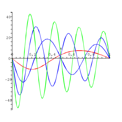
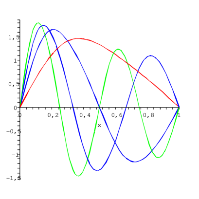
Fig. 1: The deformation of the shapes of the potential and WF of the bound state at the level with the number $m$, coincident with the energy of factorization, in dependence on a change of the number $m$ (values $m=1,2,3,4$ at $\lambda_{m}=1$ are used): (a) — the deformation of the potential; (b) — the deformation of WF.

In the first figure (a) one can see, that the selected level $m$ determines number of intersections of the potential with axis $x$ (or number of “zero-points” of this potential); increasing it, one can increase the number of such points of intersections. We also see, that by increasing $m$ both an angle of a slope of the potential in its leaving from the left boundary at point $x=0$, and an angle of a slope of WF at its leaving from this boundary, increase (that follows from the choice of the definition of the function $I_{m}(x)$ for calculation of the deformed WFs and the potential). From these figures one can see, that at the selected values of the parameter $\lambda_{m}$ there are no any divergence on the whole region $x\in[0,a]$ both in the deformed potential, and in WF at the different values $m$, and also that WF equals to zero at the boundary points $x=0$ and $x=a$ (that points out the bounding of this state). It demonstrates an appropriateness of the method from sec. 5.1 for construction of new isospectral potentials using the superpotential, defined on the basis of WF of not only the ground state at $m=1$, but also the arbitrary excited state at $m\neq 1$.

The deformation of the potential at the change of the parameter $\lambda_{m}$ is shown in Fig. 2.

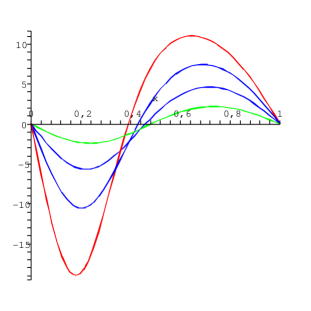
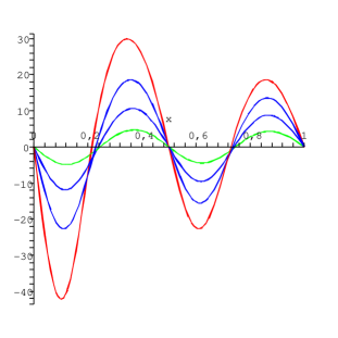
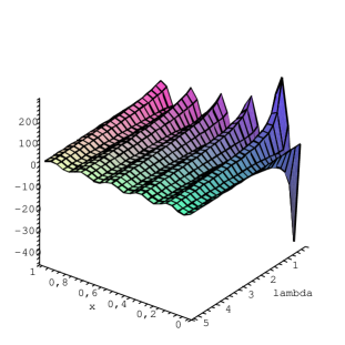
Fig. 2: The deformation of the potential at the change of the parameter $\lambda_{m}$ (the values $\lambda_{m}=0.5,1,2,5$ are used): (a) — at $m=1$, (b) — at $m=2$, (c) — the shape of the potential is deformed continuously at the change of the parameter $\lambda_{m}$ (without the divergences)

In the first figure (a) we see, how the potential is deformed, if as the energy of factorization the lowest level at $m=1$ is used. Here, we note the following:

• We see, that this figure qualitatively looks like Fig. 1 (a) from [47] (see p. 917), in which the deformation of such potential by help of the methods of the inverse problem is shown (here, varying the parameter $\lambda_{1}$ and changing the definition of the function $I_{m}(x)$, one can obtain a full similarity between these figures).

• We see, that the increase of the slope of leaving of the potential in the left wall (and the increase of minimums and maximums of the potential) at increasing of the parameter $\lambda_{1}$ coincides with the increase of the slope of leaving of the potential in the right wall (and with the increase of its minimums and maximums) in Fig. 1 (a) in [47] (see p. 917), which was caused by a change of the derivative $\gamma_{1}$ of WF of the ground state in the right wall at $x=a$. It points out a similarity between the parameter $\lambda_{1}$ in the considered method in the frameworks of SUSY QM and the coefficient $\gamma_{1}$ in the approach of the inverse problem.

• The following property is fulfilled: the deformed curves of the potential $V_{1}(\lambda_{m})$ at the different values $\lambda_{m}$ intersect the axis $x$ at different points, i. e. we obviously observe a displacement of the central zero-point of the potential at its deformation by $\lambda_{m}$. It is explained clearly (and at first time) by the found property from sec. 6.1, and this property is observed also in Fig. 1 (a) in [47] (see p. 917) (the considered node is the node of the second type, its coordinate is determined by equation (102) at the given $\lambda_{m}$).

In the second figure (b) we show the deformation of the well, if in the definition of the energy of factorization the level of the first excited state at $m=2$ is used. Here, we note the following:

• The deformed well after its mirror reflection coincides practically with Fig. 1 (5) from [47] (see p. 917), where the deformation of such well, obtained by the methods of the inverse problem at the change of the derivative $\gamma_{2}$ of WF of the first excited state at the right wall at $x=a$, is shown.

• One can see, that the increase of the leaving slope of the potential in the left wall, caused by increasing the parameter $\lambda_{2}$, coincides with the increase of the leaving slope of the potential in the right wall in Fig. 1 (5) in [47] (see p. 917), caused by a change of the derivative $\gamma_{2}$. It proves the conclusion about that the parameters $\lambda_{m}$ with the different $m$ in the method from 5.1 play the same role in the deformation of the potential, as the coefficients $\gamma_{m}$ (defined at the same levels with the numbers $m$) in the approach from [47].

• From the figure one can see, that the well after its deformation has “zero-points” of both types, described in sec. 6.1 (this property has observed and explained at the first time):

  • three zero-points, located at points of the walls of the well and at its center, which are not displaced under the change of $\lambda_{m}$ (they coincide with all nodes of WF of the first excited state at $m=2$; coordinates of these zero-points can be found from (101));

  • two zero-points, located between the previous three zero-points, which are displaced under the change of $\lambda_{m}$ (their coordinates can be found from (102) at the given $\lambda_{m}$).

  As we see, this property is displayed also in Fig. 1 (5) in [47] (see p. 917).

According to the figures (a,b), the $m$ is larger, the number of zero-points on the region $x\in[0,a]$ is larger and the displacement of zero-points of the second type in the deformation of the well is smaller.

Now let’s analyze, how the shape of WF is deformed at the level with the number $m$, coincident with the energy of factorization. In Fig. 3 such deformation of WF at the change of the number $m$ of such level is shown.

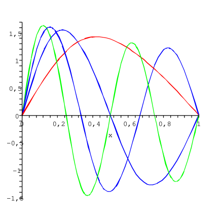
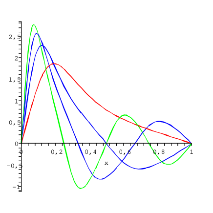
Fig. 3: The deformation of the shape of WF at the level with the number $m$, coincident with the energy of factorization, caused by the change of the number $m$ (the values $m=1,2,3,4$ are used): (a) — at $\lambda_{m}=2$; (b) — at $\lambda_{m}=0.1$

From the figures one can see the following:

• Distances between arbitrary two neighboring nodes of WF with the arbitrary number $m$ are equal, they decrease at increasing of the number $m$ and their coordinates can be found from (97) (with substitution of index $n$ into $m$).

• For any $m$ at decreasing of the module of $\lambda_{m}$ a relative weight (amplitude) of WF near one wall is increased and near another wall is decreased, at $\lambda_{m}\to\pm\infty$ a smoothing of the deformation of WF takes place and WF tends to its undeformed form.

In Fig. 4 a dependence of the shape of WF at the level with the number $m$, coincident with the energy of factorization, on the parameter $\lambda_{m}$ is shown.

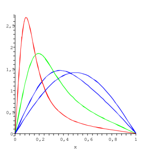
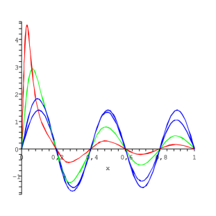
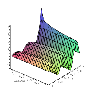
Fig. 4: The deformation of the shape of WF of the bound state at the level with the number $m$ at changing of the parameter $\lambda_{m}$ (at $\lambda_{m}=1,2,3,4$): (a) — for the ground state at $m=1$; (b) — for the state at $m=5$; (c) — the shape of WF is deformed continuously (without divergences) at change of the parameter $\lambda_{m}$

In the first figure (a) the deformation of WF of the ground state at $m=1$ is shown. We see, that this figure after mirror reflection looks like Fig. 1 (2) in [47] (see p. 917), where the deformation of WF of the ground state, caused by the methods of the inverse problem at change of the derivative $\gamma_{1}$ of this WF in the right wall, is shown! Here, we reproduce explicitly a demonstration of a deforming property of this WF, which was described in [47] (see p. 917–918, and obtained by the approach of the inverse problem): “… acceleration of increase of $\Phi_{1}$ with moving off from $x=a$ must be compensated by quicker passing to falling, because the integral from the square of wave function of the ground state remains normalizable to one. Just the hollow of the potential near $x=a$ provides such a behavior $\Phi_{1}(x)$ … But, further, it needs to compel the function, with not changing a sign, — nodes for the ground state are unallowed, — to tend to zero at point $x=0$. This is achieved by reflected part of addition to the initial potential in the left part of the well: under the barrier the function is smaller essentially then unperturbed one.” (in original text: “… ᪮७ $\Phi_{1}$ 㤠 $x=a$ ᪮ ஢ 室 ᯠ , ⮡ ⥣ࠫ 㭪樨  ̵᭮ ﭨ ⠢ ନ஢ .  ̵ࠧ 㣫㡫㭨 ⥭樠 $x=a$ ᯥ稢 ⠪ $\Phi_{1}(x)$ … 㦭 ⠢ 㭪 , , — 㧫  ̵᭮ ﭨ 饭 , — 窥 $x=0$. ⨣ ⠫ 饩 室 ⥭樠 : ஬ 㭪 ⢥ 饭 .”). Note, that increase of the slope of WF in the left wall (and, correspondingly, decrease in the right wall) at decreasing of the parameter $\lambda_{1}$ in Fig. 4 (a) coincides with increase of the slope of WF in the right wall (and, correspondingly, with decrease in the left wall) at changing of $\gamma_{1}$ in Fig. 1 (2) in [47] (a possibility to change the angle of the slope of WF at $x$-coordinates of the walls is proved analytically in sec. 6.3). In the second figure (b) the deformation of the shape of WF at the level with the number $m=5$ is shown. Here, we note the following:

• We see, that the deformation of this WF looks qualitatively like the deformation of WF of the first excited state in Fig . 1 (7) from [47], caused by change of the derivative $\gamma_{2}$ in the right wall (with taking into account of decrease of $m$). From here one can see, that the parameters $\lambda_{m}$ in the method from 5.1 play the same role in the deformation of WF as coefficients $\gamma_{m}$ (defined at the same levels) in the approach from [47].

• All deformed curves of WF with the selected number $m$ at the different values of the parameter $\lambda_{m}$ intersect through the same points — the nodes of the undeformed WF of the form (97). These nodes of WF are not displaced at change of the parameter $\lambda_{m}$, two external nodes are located at $x$-coordinates of the walls and total number of the nodes equals to $m+1$. This property is confirmed analytically by our formula (108) and it is observed in Fig. 1 (2, 7) in [47].

Now let’s consider, how the shape of WF of the ground state can be deformed, if in definition of the energy of factorization the level of the excited state at $m\neq 1$ is used. In Fig. 5 the deformation of the shape of WF of the ground state at change of the number $m$ of the level, coincident with the energy of factorization (a), and at change of the parameter $\lambda_{m}$ at $m=2$ (b) and at $m=3$ (c), is shown.

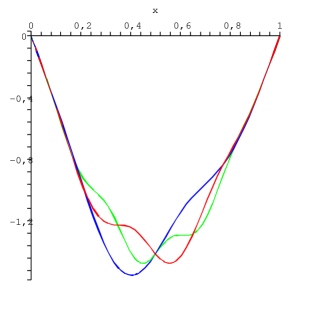
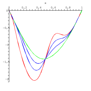
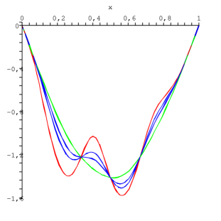
Fig. 5: The deformation of the shape of WF of the ground bound state: (a) — at change of the number $m$ of the level, coincident with the energy of factorization ($m=2,3,4$ at $\lambda_{m}=1$); (b) — at change of the parameter $\lambda_{2}$ ($\lambda_{2}=0.01,0.3,1,10$, at definition of the energy of factorization the level with the number $m=2$ is used); (c) — at change of the parameter $\lambda_{3}$ ($\lambda_{3}=0.1,0.5,1,10$, at definition of the energy of factorization the level with the number $m=3$ is used)

In the first figure (a) the deformation of WF of the ground state at change of the number $m$ is shown (such a case of deformation is absent in [47] see p. 917). Here, we note the following:

• increase of the number $m$ by 1 introduces one new perturbation (or “oscillation) into the shape of WF;

• angles of leaving of WF of the ground state at points of the right and left walls keep safe at change of the number $m$, that demonstrates clearly properties 2 found in sec. 6.4.

In the second figure (b) the deformation of WF of the ground state at change of the parameter $\lambda_{2}$ at $m=2$ is shown. We see, that this figure after mirror reflection coincides with Fig. 1 (6) from [47] (see p. 917), where the deformation of WF of the ground state, caused by the methods of the inverse problem on the basis of change of the derivative $\gamma_{2}$ of WF of the first excited state in the right wall, is shown. Comparing these figures, we conclude:

• angles of leaving of WF of the ground state at points of the right and left walls at change of the parameter $\lambda_{2}$ in the method from 5.1 and at change of the coefficient $\gamma_{2}$ in the method of the inverse problem from [47] are not changed — this demonstrates the properties 2 found in sec. 6.4;

• there is only one point, in which all deformed curves of WF of the ground state intersect between themselves and with the undeformed curve of this WF (without coordinates of the walls); the coordinate of this point is located exactly in the center of the well and coincides with the node of WF of the first excited state with the number $m=2$, and also with zero-point of the first type of the deformed potential, — this visibly demonstrates properties 1 found in sec. 6.4 (this is the point of the first type);

• there is the same increase of the angle between curves of the deformed WF and undeformed WF at point of their intersection (in the center of the well) at decreasing of the parameter $\lambda_{2}$ in the method from sec. 5.1 and at change of the coefficient $\gamma_{2}$ in the approach of the inverse problem from [47].

In the third figure (c) the deformation of WF of the ground state at change of the parameter $\lambda_{3}$ at $m=3$ is shown, from here one can see, that all considered above properties of the deformation of WF at $m=2$ are carried out and in this case (however, here WF has three points, in which it is not deformed: besides two points of the first type, the coordinates of which coincide with the nodes of WF of the excited state at the level with the number $m=3$, which coincides with the energy of factorization, else one point of the second type appears in the center of the well, that confirms the properties 1 from sec. 6.4). From analysis of all figures one can conclude the following:

• For arbitrary selected level with the number $m$, coincident with the energy of factorization, there are different numbers of the points of intersection between the deformed curves for the same WFs (using the parameter $\lambda_{m}$) for other levels with the other numbers then $m$ (it confirms the properties found in sec. 6.4 and formula (112) for coordinates of these points).

• If the numbers $m$ and $n$ determine the number of oscillations of the curve of the deformed WF relatively its undeformed form, then using $\lambda_{m}$ one can reinforce or enfeeble amplitude of these oscillations.

The deformation of WF of the first excited state is shown in Fig. 6.

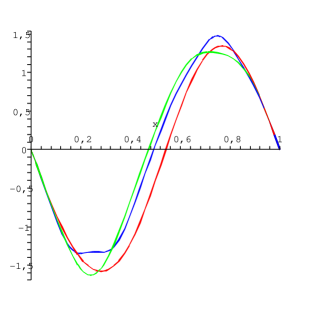
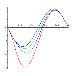
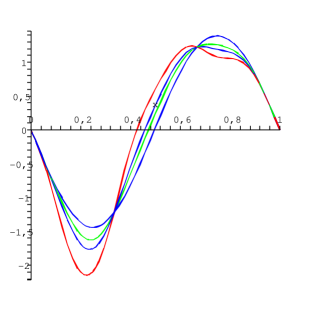
Fig. 6: The deformation of the shape of WF of the first excited state: (a) — at change of the number $m$ of the level of the deformation ($m=1,3,5$, at $\lambda_{m}=1$); (b) — at change of the parameter $\lambda_{m}$ ($\lambda_{m}=0.01,0.3,1,10$, in definition of the energy of factorization the level with the number $m=1$ is used); (c) — at change of the parameter $\lambda_{m}$ ($\lambda_{m}=0.1,0.5,1,10$, in definition of the energy of factorization the level with the number $m=3$ is used)

In the first figure (a) the deformation of this WF at change of the number $m$ of the level is shown (there is no such a case in Fig. 1 in [47], see p. 917). We see, that a behavior of this WF in such deformation looks like WF of the ground state (see Fig. 5 (a)):

• increase of the number $m$ by 1 introduce one new perturbation (or “oscillation) into the shape of WF;

• angles of leaving of WF of the ground state at points of the right and left walls are not changed under change of the number $m$.

In the second figure (b) the deformation of WF of the first excited state at change of the parameter $\lambda_{1}$ at $m=1$ is shown. We see, that this figure at mirror reflection coincides with Fig. 1 (3) in [47] (see p. 917), where the deformation of WF of the first excited state, caused by change of the derivative $\gamma_{1}$ of WF of the ground state in the right wall using the methods of the inverse problem, is shown. Comparing these figures, we conclude:

• angles of leaving of WF of the first excited state at points of the right and left walls at change of the parameter $\lambda_{1}$ in the method from 5.1 and at change of the coefficient $\gamma_{1}$ in the method of the inverse problem from [47] are not changed;

• curves of the deformed WFs at change of $\lambda_{1}$ in the method from 5.1 and at change of $\gamma_{1}$ in the method of the inverse problem from [47] are not intersected (it agrees with the formula (112)).

From the third figure (c) one can see, that the considered above properties of the deformation of WF of the ground state at change of $\lambda_{m}$ at the selected number $m$, are fulfilled also for WF of the excited state (with increasing of $m$, the number of points of intersections of the deformed curves of WF between themselves and with the undeformed shape of this WF for each selected excited state is increased, that follows also from (112)).

In Fig. 7 one can see, which forms the deformed potential (a) and its WF of the bound state (b) at the level with a larger number $m$, coincident with the energy of factorization, have (the value $m=15$ is chosen).

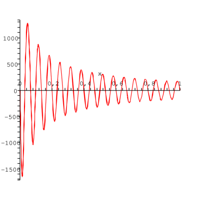
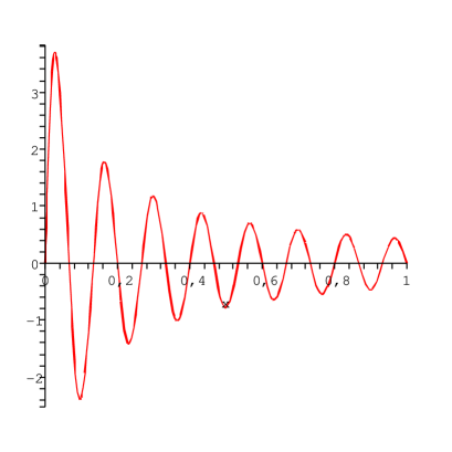
Fig. 7: Shapes of the potential (a) and its WF of the bound state (b) at the level, coincident with the energy of factorization, at $m=15$ and $\lambda_{m}=0.1$

Conclusions:

Using the supersymmetric method from sec. 5.1, we have obtained all pictures of the deformation (without displacement of the levels in the spectrum) for the rectangular well with infinitely high walls and its WFs of the lowest bound states, which were obtained early in the review [47] (see p. 916–919) on the basis of the methods of the inverse problem. Note the following:

• Appropriateness of the method from sec. 5.1 for construction of new isospectral potentials on the basis of one given potential $V_{1}$ in the form of the rectangular well with infinitely high external walls has proved (one can consider such a method as the method of deformation of the given $V_{1}$), in which for definition of the function of factorization in the construction of the superpotential the WF of arbitrary excited bound state (but not the ground state only) is used. All possible divergences in the found solutions can be excluded by change of the parameter $\lambda_{m}$ inside one from regions in (117).

• The parameter $\lambda_{m}$ with arbitrary number $m$ of the level for the bound state in the supersymmetric method from 5.1 plays the same role in the deformation of the potential and its WFs, as the derivative $\gamma_{m}$ of WF of the bound state at the same level at point of one from the boundaries of the potential, which is used for the deformation of the potential and its WFs by the methods of inverse problem (see [47] p. 917–927) (it has obtained at the first time).

• Let’s summarize, how WFs of the different bound states are changed under the deformation by the parameter $\lambda_{m}$:

  For WF at the arbitrary level with the number $m$, coincident with the energy of factorization:

  • WF has $m+1$ nodes exactly, which are not displaced under change of $\lambda_{m}$ and coincide with the nodes of the undeformed WF (96);

  • $x$-coordinates $x=0$ and $x=a$ of the walls are such nodes also;

  • angles of leaving of this WF at points of the right and left walls are changed at the deformation.

  For WF of the other bound state at the level with arbitrary number $n$, not coincident with the energy of factorization ($n\neq m$):

  • There are such points, in which all deformed curves of such WF intersect between themselves and with the undeformed WF (i. e. these points are not displaced at change of the parameter $\lambda_{m}$). This property (at the first time has been confirmed analytically by formulas (108) and (111)–(112), with taking into account the next point in these Conclusions) gives an answer on a question, stated in [47] (see p. 918): “it is not clear, why the functions $\Phi_{1}(x)$ and $\Phi_{2}(x)$ (i. e. WFs of the ground and the first excited states) at all values (i. e. in any deformation using the coefficient $\gamma_{2}$ — as analogue of $\lambda_{2}$ in the methods of the inverse problem) pass through only one point in the center of the well” (in the original text: “  ̵᭮ ⠪ , 祬 㭪樨 $\Phi_{1}(x)$ $\Phi_{2}(x)$ 祭 室 १ 業 ”).

  • One can devide all these points into two types:

    • The points of the first type, $x$-coordinates of which equal to (113) and coincide with the nodes (97) or (108) of WF of the bound state at the level with the number $m$, which coincides with the energy of factorization, and also with zero-points of the first type of the form (101) of the potential.

    • The points of the second type, coordinates of which do not coincide with the nodes of WF of the bound state at the level with the number $m$, which coincides with the energy of factorization. The coordinates of these points are determined from the second equation of the system (112).

  • The boundary points $x=0$ and $x=a$ are such points both the first type, and the second one.

  • WF of arbitrary bound state (at its deformation using the parameter $\lambda_{m}$) has exactly $m+1$ such points of the first type, and number of the points of the second type which can be determined from the second equation of (113).

  • Angles of leaving of such WF at points $x=0$ and $x=a$ of the walls are not changed under the deformation of this WF, caused by change of the parameter $\lambda_{m}$ (or by change of the coefficient $\gamma_{m}$ in the methods of the inverse problem) — in contrast to WF of the state with the number $m$! This property (at the first time has been confirmed analytically in sec. 6.4) gives an answer on a question, stated in [47] (see p. 918): how to explain an invariable slope of WF at $x$-coordinates of the walls under its deformation by the coefficient $\gamma_{2}$ using the method of the inverse problem.

• Now let’s summarize, how the shape of the well is deformed under change of the parameter $\lambda_{m}$ with the fixed number $m$.

  According to (100), one can divide all zero-points of the potential (i. e. the points of the intersection of the potential with axis $x$) into two types (for the deformed rectangular well this property has been revealed and has been explained at the first time):

  • Zero-points of the first type, which coincide with the nodes of WF of the bound state at the level with the number $m$, which coincides with the energy of factorization. These zero-points are not displaced under the deformation of the potential by the parameter $\lambda_{m}$ and their coordinates are determined from (101).

  • Zero-points of the second type, which do not coincide with the nodes of WF of the bound state at the level with the number $m$, which coincides with the energy of factorization. These points are displaced under the deformation of the potential by the parameter $\lambda_{m}$ and their coordinates are determined from (102).

7 Construction of new potentials, where unbound state is used in definition of the function of factorization

On the example of the deformation of the rectangular well we have seen, that the supersymmetric method (with taking into account not only ground bound states, but excited ones also in construction of the superpotential) allows to obtain a whole variety of the deformations (without displacement of levels in spectrum), which were obtained early by the methods of the inverse problem.

It turns out, that if to do not restrict oneself by the bound states only in the definition of the superpotential, but to construct it using a function (we shall name it as WF of the unbound state), which is a general solution (without implying of boundary conditions) of the Schrödinger equation with the starting potential $V_{1}$ at arbitrary selected energy level (which can be not coincident with the energy levels of the potential $V_{1}$), then one can obtain new exactly solvable potentials (which have own energy spectra with the bound states). Such a way for the construction of the superpotential enlarges further a class of exactly solvable potentials with only one given starting $V_{1}$ (and gives more rich possibilities for the deformation of $V_{1}$), which was obtained early by the method from Sec. 5.1–5.2. In particular, one can construct a new potential, energy spectrum of which is shifted in accordence with a chosen rule relatively the energy spectrum of the starting potential $V_{1}$ (that has not been obtained else by the other known SUSY QM methods). This points out to a possibility and advisability of development of SUSY QM methods, where in the construction of the superpotential as the energy of factorization the arbitrary energy (which can be not coincident with the energy spectrum of $V_{1}$) is used, and the function of factorization is defined concerning the unbound state at this energy. As a demonstration, further we shall present two new approaches of construction of new potentials, when as the starting potential $V_{1}$ the rectangular well with infinitely high external walls in the form (90) is used.

Let’s consider an arbitrary unbound state at an arbitrary selected level of the energy spectrum of the rectangular well $V_{1}$. We denote these WF and the level by index $n$. One can write such WF in a form (at $E_{n}^{(1)}\geq 0$):

$$\varphi_{n}^{(1)}(x)=C_{n}\sin(k_{n}x+\delta_{n}),$$ (118)

where $k_{n}$ is a wave vector, corresponding to the level $E_{n}$ ($k_{n}^{2}=E_{n}$), $C_{n}$ and $\delta_{n}$ are constants, which have complex values.

Choosing the arbitrary energy for the definition of the energy of factorization, and WF of the unbound state at this energy for the definition of the function of factorization, we construct the superpotential (we add index $w$ to designations of such energy, its wave vector and WF):

$$W(x)=-\displaystyle\frac{d}{dx}\log{|\varphi_{w}^{(1)}|}=-\displaystyle\frac{d\sin{(k_{w}x+\delta_{w})}}{dx}\Big{/}\sin{(k_{w}x+\delta_{w})}=-k_{w}\cot{(k_{w}x+\delta_{w})}$$

or

$$W(x)=-k_{w}\cot{(k_{w}x+\delta_{w})}.$$ (119)

7.1 A potential-partner to the rectangular well with a number “up”

In the first case, we shall find a new potential $V_{2}$, which is a partner to the rectangular well with the number “up”, obtained using direct SUSY-transformation with the superpotential in the form (119).

Let’s find a form of the new potential $V_{2}$:

$$V_{2}(x)=2\displaystyle\frac{dW}{dx}=-2k_{w}\displaystyle\frac{d}{dx}\cot{(k_{w}x+\delta_{w})}=\displaystyle\frac{2k_{w}^{2}}{\sin^{2}{(k_{w}x+\delta_{w})}}$$

or

$$V_{2}(x)=\displaystyle\frac{2k_{w}^{2}}{\sin^{2}{(k_{w}x+\delta_{w})}}.$$ (120)

One can see, that:

• at $E_{w}>E_{1}^{(1)}$ the new potential $V_{2}$ has infinitely high barriers with maximums at points $x_{barrier}$:

  $$\begin{array}[]{cc}x_{barrier}=\displaystyle\frac{\pi l-\delta_{w}}{k_{w}},&\mbox{at }l=0,1,2\ldots\end{array}$$ (121)

• at $E_{w}<E_{1}^{(1)}$ (and wiht selected $\delta_{w}$) the potential $V_{2}$ becomes continuous function and has no any divergence in the region $x\in[0,a]$;

• the coordinates (121) of the divergences for $V_{2}$ coincide with the coordinates of the divergences of the superpotential (119).

However, we can take the solution (120) as the solution for the new exactly solvable potential $V_{2}$, only if it has the bound states (without the divergences). Therefore, it is important to analyze WFs of $V_{2}$.

At first, let’s analyze, which states for the new potential $V_{2}$ are possible at the level, coinciding with the energy of factorization $E_{w}$. Direct action of operator $\hat{A}_{w}=\frac{d}{dx}+W$ on wave function $\varphi_{w}^{(1)}$ at the energy $E_{w}$ gives zero solution. According to Sec. 4.2, there is the following non-normalizable solution for $V_{2}$, concerned with the function $\varphi_{w}^{(1)}$:

$$\begin{array}[]{cc}\varphi_{w}^{(2)}=\displaystyle\frac{I_{w}+\lambda_{w}}{\varphi_{w}^{(1)}},&I_{w}(x)=\displaystyle\int\limits_{-\infty}^{x}(\varphi_{w}^{(1)}(x^{\prime}))^{2}dx^{\prime},\end{array}$$ (122)

where $\lambda_{w}$ is constant. We find a function $I_{w}$:

$$\begin{array}[]{c}I_{w}(x)=\displaystyle\int\limits_{-\infty}^{x}(\varphi_{w}^{(1)}(x^{\prime}))^{2}dx^{\prime}=C_{w}^{2}\displaystyle\int\limits_{0}^{x}\sin^{2}{(k_{w}x^{\prime}+\delta_{w})}dx^{\prime}=C_{w}^{2}\displaystyle\int\limits_{0}^{x}\displaystyle\frac{1}{2}\Bigl{(}1-\cos(2k_{w}x^{\prime}+2\delta_{w})\Bigr{)}dx^{\prime}=\\ =\displaystyle\frac{C_{w}^{2}}{2}\biggl{(}x^{\prime}-\displaystyle\frac{\sin{(2k_{w}x^{\prime}+2\delta_{w})}}{2k_{w}}\biggr{)}\Biggr{|}_{x^{\prime}=0}^{x^{\prime}=x}=C_{w}^{2}\displaystyle\frac{2k_{w}x+\sin{2\delta_{w}}-\sin{(2k_{w}x+2\delta_{w})}}{4k_{w}}\end{array}$$

or

$$I_{w}(x)=C_{w}^{2}\displaystyle\frac{2k_{w}x+\sin{2\delta_{w}}-\sin{(2k_{w}x+2\delta_{w})}}{4k_{w}}.$$ (123)

Taking into account this, we obtain:

$$\varphi_{w}^{(2)}(x)=\displaystyle\frac{C_{w}}{4k_{w}}\displaystyle\frac{2k_{w}x+\sin{2\delta_{w}}-\sin{(2k_{w}x+2\delta_{w})}+\displaystyle\frac{4k_{w}\lambda_{w}}{C_{w}^{2}}}{\sin{(k_{w}x+\delta_{w})}}.$$ (124)

The solution (124) defines bound state, if the function $\varphi_{w}^{(2)}$ is continuous in the region $x\in[0,a]$ and equals to zero at $x=0$ and $x=a$.

Let’s analyze a behavior of $\varphi_{w}^{(2)}$ at point $x=0$. At $\delta_{w}\neq\pi l$ we obtain:

$$\varphi_{w}^{(2)}(0)=\displaystyle\frac{C_{w}}{4k_{w}}\displaystyle\frac{4k_{w}\lambda_{w}}{C_{w}^{2}\sin{\delta_{w}}}=\displaystyle\frac{\lambda_{w}}{C_{w}\sin{\delta_{w}}}.$$

One can see, that at $\delta_{w}\neq\pi l$ the function $\varphi_{w}^{(2)}$ equals to zero at $\lambda_{w}=0$ only. At $\delta_{w}=\pi l$, the function $\varphi_{w}^{(0)}(0)$ equals to zero also at $\lambda_{w}=0$. In deed, we find:

$$\begin{array}[]{lcl}\varphi_{w}^{(2)}(0)&=&\displaystyle\frac{C_{w}}{4k_{w}}\displaystyle\frac{2k_{w}\Bigl{(}1-\cos{(2k_{w}x+2\delta_{w})}\Bigr{)}}{k_{w}\cos{(k_{w}x+\delta_{w})}}\Biggr{|}_{x\to 0}=\displaystyle\frac{C_{w}}{2k_{w}}\displaystyle\frac{1-\cos{2\delta_{w}}}{\cos{\delta_{w}}}=\displaystyle\frac{C_{w}}{2k_{w}}\displaystyle\frac{1-1}{(-1)^{l}}=0.\end{array}$$

We write down values $\delta_{w}$ and $\lambda_{w}$, when the function $\varphi_{w}^{(2)}$ equals to zero at point $x=0$:

$$\begin{array}[]{ccc}\lambda_{w}=0,&\delta_{w}\mbox{ is arbitrary},&k_{w}\mbox{ is arbitrary }(k_{w}\neq 0).\end{array}$$ (125)

Now let’s analyze a behavior of the function $\varphi_{w}^{(2)}$ at point $x=a$. If $k_{w}a+\delta_{w}\neq\pi l$, then from (124) at $\lambda_{w}=0$ we obtain a condition, when the function $\varphi_{w}^{(2)}$ equals to zero:

$$2k_{w}a+\sin{2\delta_{w}}-\sin{(2k_{w}a+2\delta_{w})}=0.$$ (126)

Such dependence defines a needed value of the phase $\delta_{w}$ at selected $k_{w}$, which can be arbitrary. At $k_{w}a+\delta_{w}=\pi l$ the function $\varphi_{w}^{(2)}(a)$ equals to zero only at

$$\lambda_{w}=-\displaystyle\frac{C_{w}}{4k_{w}}\Bigl{(}2k_{w}a+\sin{2\delta_{w}}\Bigr{)}=0.$$ (127)

In deed, we find:

$$\begin{array}[]{lcl}\varphi_{w}^{(2)}(a)&=&\displaystyle\frac{C_{w}}{4k_{w}}\displaystyle\frac{2k_{w}\Bigl{(}1-\cos{(2k_{w}x+2\delta_{w})}\Bigr{)}}{k_{w}\cos{(k_{w}x+\delta_{w})}}\Biggr{|}_{x\to a}=\displaystyle\frac{C_{w}}{2k_{w}}\displaystyle\frac{1-1}{(-1)^{l}}=0.\end{array}$$

From (127) we obtain the necessary condition for $k_{w}$:

$$\sin{2\delta_{w}}=-2k_{w}a.$$ (128)

In this case the function $\varphi_{w}^{(2)}$ equals to zero at point $x=a$ at some values of $k_{w}$ and $\delta_{w}$.

We write down such values of $\delta_{w}$ and $\lambda_{w}$, when the function $\varphi_{w}^{(2)}$ equals to zero at points $x=0$ and $x=a$ with selected $k_{w}$, which can be arbitrary:

$$\begin{array}[]{lllll}1)&k_{w}a+\delta_{w}\neq\pi l,&2k_{w}a+\sin{2\delta_{w}}-\sin{(2k_{w}a+2\delta_{w})}=0,&\lambda_{w}=0;\\ 2)&k_{w}a+\delta_{w}=\pi l,&\sin{2\delta_{w}}=-2k_{w}a,&\lambda_{w}=0,\end{array}$$ (129)

where $l=0,1,2\ldots$.

At second, let’s find WF of the arbitrary (unbound) state for $V_{2}$ at the level $E_{n}$ with the number $n$, not coinciding with the energy of factorization:

$$\begin{array}[]{c}\varphi_{n}^{(2)}(x)=\bar{C}_{n}\hat{A}_{w}\varphi_{n}^{(1)}=\bar{C}_{n}\biggl{(}\displaystyle\frac{d}{dx}+W\biggr{)}\varphi_{n}^{(1)}=\\ =\bar{C}_{n}C_{n}\Bigl{(}k_{n}\cos{(k_{n}x+\delta_{n})}-k_{w}\cot{(k_{w}x+\delta_{w})}\sin{(k_{n}x+\delta_{w})}\Bigr{)}\end{array}$$

or

$$\varphi_{n}^{(2)}(x)=\bar{C}_{n}C_{n}\Bigl{(}k_{n}\cos{(k_{n}x+\delta_{n})}-k_{w}\cot{(k_{w}x+\delta_{w})}\sin{(k_{n}x+\delta_{n})}\Bigr{)},$$ (130)

where $\hat{A}_{w}=\frac{d}{dx}+W$, $\bar{C}_{n}$ is arbitrary constant, which we shall use instead of the factor $|E_{n}^{(1)}-E_{w}^{(1)}|^{-1}$, because we consider the non-normalizable state.

In order to the function (130) describes the bound state, it needs, that it must be continuous in the region $x\in[0,a]$ and equals to zero at points $x=0$ and $x=a$. Let’s analyze, when this function can be continuous. According to (130), the divergences appear at point $x_{break}$ at

$$\sin{(k_{w}x_{break}+\delta_{w})}=0.$$ (131)

However, if at all points $x_{break}$ the following condition is fulfilled:

$$\sin{(k_{n}x_{break}+\delta_{n})}=0,$$ (132)

then the function (130) is continuous and has no divergences. In deed, assuming, that the conditions (131) and (132) are fulfilled at point $x=x_{break}$, we analyze the second item of the function (130) at this point. We obtain:

$$\begin{array}[]{c}-k_{w}\cot{(k_{w}x_{break}+\delta_{w})}\sin{(k_{n}x_{break}+\delta_{n})}=-k_{w}\displaystyle\frac{\cos{(k_{w}x+\delta_{w})}\sin{(k_{n}x+\delta_{n})}}{\sin{(k_{w}x+\delta_{w})}}\Biggr{|}_{x\to x_{break}}=\\ =k_{w}\displaystyle\frac{k_{w}\sin{(k_{w}x+\delta_{w})}\sin{(k_{n}x+\delta_{n})}-k_{n}\cos{(k_{w}x+\delta_{w})}\cos{(k_{n}x+\delta_{n})}}{k_{w}\cos{(k_{w}x+\delta_{w})}}\Biggr{|}_{x\to x_{break}}=\\ =-k_{w}\displaystyle\frac{k_{n}\cos{(k_{w}x_{break}+\delta_{w})}\cos{(k_{n}x_{break}+\delta_{n})}}{k_{w}\cos{(k_{w}x_{break}+\delta_{w})}}=-k_{n}\cos{(k_{n}x_{break}+\delta_{n})}=(-1)^{l+1}k_{n}.\end{array}$$

Continuity condition of WF: the function $\varphi_{n}^{(2)}(x)$, describing a state with number $n$ and having the form (130), is continuous in the region $x\in[0,a]$, if each point $x_{break}$, defined by (131) at selected $k_{w}$ and $\delta_{w}$, satisfies to the condition (132) for the corresponding $k_{n}$ and $\delta_{n}$. According to (130), such points $x_{break}$ are nodes of this WF (at even $l$).

Now let’s find out, when the function (130) equals to zero at points $x=0$ and $x=a$. From a condition of equality to zero we obtain:

$$\begin{array}[]{lcl}(x=0)&\to&k_{n}\cos{\delta_{n}}-k_{w}\cot{\delta_{w}}\sin{\delta_{n}}=0;\\ (x=a)&\to&k_{n}\cos{(k_{n}a+\delta_{n})}-k_{w}\cot{(k_{w}a+\delta_{w})}\sin{(k_{n}a+\delta_{n})}=0.\end{array}$$ (133)

Let’s $\cos{\delta_{w}}\neq 0$. From the first equation we obtain:

$$\begin{array}[]{ccc}\tan{\delta_{n}}=\displaystyle\frac{k_{n}}{k_{w}}\tan{\delta_{w}},&\cos{\delta_{n}}\neq 0,&\cos{\delta_{w}}\neq 0.\end{array}$$ (134)

Rewrite the second equation of the system (133) by such a way:

$$\begin{array}[]{lcl}k_{n}\cos{\delta_{n}}\Bigl{(}\cos{k_{n}a}-\displaystyle\frac{k_{n}}{k_{w}}\sin{k_{n}a}\tan{\delta_{w}}\Bigr{)}=\par k_{w}\cot{(k_{w}a+\delta_{w})}\cos{\delta_{n}}\Bigl{(}\sin{k_{n}a}+\displaystyle\frac{k_{n}}{k_{w}}\cos{k_{n}a}\tan{\delta_{w}}\Bigr{)}.\end{array}$$ (135)

From here we obtain:

$$\tan{k_{n}a}=\displaystyle\frac{k_{n}}{k_{w}}\displaystyle\frac{1-\cot{(k_{w}a+\delta_{w})}\tan{\delta_{w}}}{\cot{(k_{w}a+\delta_{w})}+\displaystyle\frac{k_{n}^{2}}{k_{w}^{2}}\tan{\delta_{w}}}.$$ (136)

Transform this equation so:

$$\tan{k_{n}a}=\displaystyle\frac{k_{n}}{k_{w}}\displaystyle\frac{\sin{k_{w}a}}{\cos{(k_{w}a+\delta_{w})}\cos{\delta_{w}}+\displaystyle\frac{k_{n}^{2}}{k_{w}^{2}}\sin{(k_{w}a+\delta_{w})}\sin{\delta_{w}}}.$$ (137)

In contrast to (136), numerator and denominator of the right part of the equation (137) have no any infinitely large value at arbitrary $k_{n}$, $k_{w}$ ($k_{w}\neq 0$) and $\delta_{w}$. Such expression is more convenient for analysis of zeros.

Now let’s consider a case $\cos{\delta_{w}}=0$. From (133) we obtain instead of the equations (134) an (137) the following:

$$\begin{array}[]{ccc}\tan{k_{n}a}=\displaystyle\frac{k_{w}}{k_{n}}\tan{k_{w}a},&\cos{\delta_{n}}=0,&\cos{\delta_{w}}=0.\end{array}$$ (138)

We see, that the equations (137) are (138) transcendental and in a general case it needs to resolve each from them numerically, that makes a problem of obtaining of new types of exactly solvable potentials as very difficult. In result, we shall obtain a spectrum of all possible values of $k_{n}$ (energy spectrum $E_{n}^{(2)}$) in dependence on selected values of $k_{w}$ and $\delta_{w}$. However, some partial solutions of the new potentials (with WFs and energy spectra, in the explicit form) can be found more simply. Let’s consider two cases.

7.1.1 New isospectral potentials with shift of their shape along axis $x$

In the first case, let’s assume, that all energy levels of the new potential $V_{2}$ coincide with the levels of the spectrum of the rectangular well $V_{1}$. Then we have:

$$\sin{k_{n}a}=0.$$ (139)

From (137) at $\cos{\delta_{w}}\neq 0$ or from (138) at $\cos{\delta_{w}}=0$ we obtain:

$$\sin{k_{w}a}=0.$$ (140)

We see, that the energy of factorization $E_{w}$ coincides with one level from the spectrum $E_{n}^{(1)}$ for the rectangular well (we have an arbitrariness in a choice of the parameter $\delta_{w}$).

Now we assume, that the new potential $V_{2}$, in addition to the found energy spectrum, has some other levels. From (138) we see, that at $\delta_{w}=\frac{\pi}{2}+\pi l$ it is not possible ($l=0,1,2\ldots$). At $\delta_{w}\neq\frac{\pi}{2}+\pi l$ equation (137) can give such solution. As we found early, the level $E_{w}$ belongs to the spectrum $E_{n}^{(1)}$, therefore: $\sin{k_{w}a}=0$. From (137) we obtain:

$$k_{n}^{2}=-k_{w}^{2}\cot^{2}{\delta_{w}}.$$ (141)

As for WF of the starting potential we have chosen the solutions (118) at the levels $E_{n}^{(1)}>0$, then $k_{n}^{2}>0$ and $k_{w}^{2}>0$. Therefore, the solution (141) is possible only at complex values of $\delta_{w}$ (at $Im\delta_{w}\neq 0$). The complex phase $\delta_{w}$ gives complex values of the superpotential $W$ and can lead to new types of SUSY-transformations (which one can find in literature).

Taking into account the found energy spectrum for the potential $V_{2}$, the condition of continuity of WF of the bound state with the number $n$ leads to the following additional interdependence between the phases $\delta_{w}$ and $\delta_{n}$ ($w$ is the number of the level $E_{w}$ in the spectrum $E_{n}^{(2)}$):

$$\begin{array}[]{cc}\delta_{n}=\displaystyle\frac{n}{w}\delta_{w}+2\pi l,&l=0,1,2\ldots\end{array}$$ (142)

Conclusion: At the real phase $\delta_{w}$, the new potential $V_{2}$ has the energy spectrum $E_{n}^{(2)}$, coinciding completely with the energy spectrum $E_{n}^{(1)}$ of the rectangular well (with possible exclusion of one level $E_{w}$). At $E_{w}=E_{1}^{(1)}$ (at $k_{n}=nk_{w}$) we have the following:

• At $\delta_{w}=\pi l$ ($l=0,1,2\ldots$) the potential $V_{2}$ coincides with the potential (24) from [6] without shift down by value $\Delta E=E_{1}=\frac{\hbar^{2}\pi^{2}}{2mL^{2}}$ (see p. 278–279, Fig. 2.2; for exact comparison it needs to use $\hbar=1$, $2m=1$, $L=a$, $n_{\mbox{\scriptsize my}}=n_{\mbox{\tiny Cooper, Khare, Sukhatme}}+1$, and we obtain the potential and spectrum without displacement: $V_{2}=\frac{\hbar^{2}\pi^{2}}{mL^{2}}\mbox{cosec}^{2}{(\pi x/L)}$, $E_{n}=\frac{\hbar^{2}\pi^{2}}{2mL^{2}}n^{2}$).

  • In contrast to [6] (see p. 278–279), we connect the potentials $V_{1}$ and $V_{2}$ by SUSY-transformation with non-zero lowest level $E_{1}\neq 0$ ($E_{1}\neq 0$  [6]).

  • At $\delta_{n}=\pi l$ the condition (142) is fulfilled jointly with (134). Therefore, WF of the form (130) is continuous in the region $x\in[0,a]$ and equals to zero at points $x=0$ and $x=a$. Therefore, a state described by this WF at arbitrary level with the number $n$ (not coincident with $E_{w}$) of the energy spectrum $E_{n}^{(2)}$ for the new potential $V_{2}$ must be bound.

  • At $\delta_{n}=\pi l$ the conditions (1) and (2) from (129) are not fulfilled (besides $k_{w}=0$). Therefore, the state for $V_{2}$ at the lowest level $E_{1}^{(1)}$ cannot be bound and we must to exclude this level from the energy spectrum of the new potential $V_{2}$ (this agrees with [6]).

• At $\delta_{w}\neq\pi l$ the potential $V_{2}$ displaces along axis $x$ (using $\delta_{w}$) with appearance of one infinitely high barrier, which has a maximum with coordinate determined from (121). Here, we have two cases:

  • At $\cos{\delta_{w}}=0$ the equation (142) is fulfilled jointly with the condition $\cos{\delta_{n}}=0$ from (138) at $\delta_{n}=\frac{\pi}{2}+\pi l$ and at arbitrary odd number $n$. This defines a bound excited state at such $n$ (continuity of WF of this state in the region $x\in[0,a]$, its zero values at points $x=0$ and $x=a$). Therefore, we obtain a new potential $V_{2}$ with infinitely high barrier, maximum of which is located exactly in the center of the well at $x_{barrier}=a/2$ and all levels of the spectrum (with the bound states) coincide with the levels with odd numbers of the spectrum $E_{n}^{(1)}$ of the starting potential $V_{1}$.

  • At $\cos{\delta_{w}}\neq 0$, for analysis of existence of excited bound states we must to analyze a compatibility of the conditions (142) and (134), that leads to the transcendental equation (134). A barrier of $V_{2}$ can be displaced along axis $x$, its maximum has a coordinate:

    $$x_{barrier}=\displaystyle\frac{\pi-\delta_{w}}{k_{w}}=a\Bigl{(}1-\displaystyle\frac{\delta_{w}}{\pi}\Bigr{)}.$$ (143)

  • There is no bound state at the level $E_{w}$ in the potential $V_{2}$. Necessary conditions (1)–(2) from (129) are not fulfilled.

7.1.2 New potentials with shift of the energy spectrum

Now let’s consider another case. We assume, that the levels of the new potential $V_{2}$ do not coincide with the levels of the energy spectrum of the starting potential $V_{1}$ and instead of the equation (139) satisfy to the following:

$$\cos{k_{n}a}=0.$$ (144)

Let’s analyze, whether the bound states in the potential $V_{2}$ with such energy spectrum are possible.

At $\cos{\delta_{w}}\neq 0$ from (137) with taking into account (144) we obtain:

$$\cos{(k_{w}a+\delta_{w})}\cos{\delta_{w}}=-\displaystyle\frac{k_{n}^{2}}{k_{w}^{2}}\sin{(k_{w}a+\delta_{w})}\sin{\delta_{w}}.$$ (145)

This equation has a solution for a spectrum of values of $k_{n}$ with different numbers $n$ at one pair of $\delta_{w}$ and $k_{w}$, if it equals to zero. From here we find:

$$\begin{array}[]{c}\Bigl{(}\cos{(k_{w}a+\delta_{w})}=0\Bigr{)}\to\Bigl{(}\sin{(k_{w}a+\delta_{w})}\neq 0\Bigr{)}\to\Bigl{(}\sin{\delta_{w}}=0\Bigr{)}\to\\ \to\Bigl{(}\cos{\delta_{w}}\neq 0\Bigr{)}\to\Bigl{(}\cos{k_{w}a}=0,\;\delta_{w}=\pi l\Bigr{)},\end{array}$$ (146)

where $l=0,1,2\ldots$.

At $\cos{\delta_{w}}=0$ from (138) with taking into account (144) we obtain:

$$\begin{array}[]{cc}\cos{k_{w}a}=0,&\delta_{w}=\displaystyle\frac{\pi}{2}+\pi l.\end{array}$$ (147)

Let’s write down a full solution:

$$\begin{array}[]{cc}\cos{k_{w}a}=0,&\delta_{w}=\displaystyle\frac{\pi}{2}l,\end{array}$$ (148)

and the energy spectrum for the new potential $V_{2}$:

$$\begin{array}[]{cc}k_{n}=\displaystyle\frac{\pi}{2a}(-1+2n),&E_{n}^{(2)}=k_{n}^{2}=\displaystyle\frac{\pi^{2}}{4a^{2}}(-1+2n)^{2},\end{array}$$ (149)

where $n=1,2,\ldots$.

If at $E_{w}$ to choose the lowest level from the found spectrum $E_{n}^{(2)}$, then one can make sure, that each level of the spectrum $E_{n}^{(2)}$ has own bound state. A form of the potential $V_{2}$ with such spectrum is shown in Fig. 8 (a), a shape of WF of the ground and first two excited states (which correspond to three lowest levels of the spectrum (149)) — in Fig. 8 (b,c). From here one can see, that these WF are continuous in the region $x\in[0,a]$ and equal to zero at points $x=0$ and $x=a$, that allows on their basis to define the bound states at three lowest levels for the potential $V_{2}$.

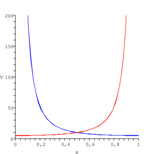
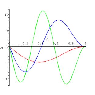
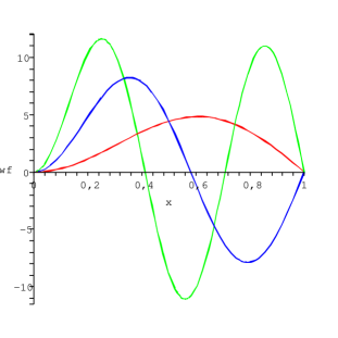
Fig. 8: The potential and its WF of the first three bound states (l=0,1,2…): (a) is a shape of the potential at $\delta_{w}=\pi/2+\pi l$ (red curve, increasing to the right) and at $\delta_{w}=\pi l$ (blue curve, increasing to the left), (b) are WFs of the first three bound states (for the first three lowest levels) at $\delta_{w}=\pi/2+\pi l$, (c) are WFs of the first three bound states at these levels at $\delta_{w}=\pi l$

Thus, the found potential $V_{2}$ in the form (120) with the parameters (148) and $k_{w}=\frac{\pi}{2a}$ is the new exactly solvable potential, which has own energy spectrum with the bound states.

Note, that the spectrum of $V_{2}$ is shifted relatively the spectrum of the rectangular well. Taking into account (93), one can write:

$$k_{n}=\displaystyle\frac{\pi n}{a}-\displaystyle\frac{\pi}{2a}=k_{n,\;well}-\displaystyle\frac{\pi}{2a},$$ (150)

where $k_{n,\;well}$ is wave vector of the rectangular well with the number $n$.

7.2 New potentials with insertion of one additional level in the spectrum

Now let’s consider another example of the deformation of the rectangular well with infinitely high walls (90). We shall use the approach for the deformation of the rectangular well in Sec. 6, where at first we fulfill using direct SUSY-transformation a transition from the rectangular well (as the starting potential $V_{1}$) into a new potential $V_{2}$ with transformation of one bound state into unbound one, and then we fulfill the inverse transition with the transformation of this unbound state into bound one, returning to the deformed “rectangular well” $V_{1}(\lambda)$. However, in contrast to the approach in Sec. 6, now in the construction of the superpotential we shall use an arbitrary energy $E_{w}$ (which can be not coincident with the levels of the spectrum for $V_{1}$) for the definition of the energy of factorization, and the general solution of WF of the unbound state at this energy for the definition of the function of factorization. So, we have the function of factorization in the form (118) (with substitution of indexes $n\to w$) and the superpotential — in the form (119).

Further, we shall restrict ourselves by finding such new potential, the energy spectrum of which coincides with the energy spectrum of the rectangular well with a possible insertion of one new level $E_{w}$. We shall consider existence of the bound states in the found potential as a condition of obtaining of the new exactly solvable potential $V_{1}(\lambda)$. Therefore, first of all for the new potential we must to analyze a form of WF of the arbitrary state at the arbitrary level $E_{n}^{(1)}$, which is not coincident with the energy of factorization $E_{w}$. One can write such WF in the form (110).

In contrast to the approach from Sec. 6, finding new solutions we shall analyze for each level of the starting potential $V_{1}$ not WF of the bound state, but a general solution of WF of the unbound state (as we do it in Sec. 7), i. e. we write such WF at the level $E_{n}^{(1)}$ with the number $n$ in the form (118).

In result, we obtain a condition of equality of WF to zero at the level $E_{n}$ for the new potential $V_{1}(\lambda)$ at points $x=0$ and $x=a$ (we write it without detailed computations):

$$\tan{\delta_{n}}=\displaystyle\frac{2k_{n}k_{w}}{|E_{n}^{(1)}-E_{w}|}\displaystyle\frac{\cos{2(k_{w}a+\delta_{w})}-\cos{2\delta_{w}}}{2k_{w}a+\Bigl{(}\sin{2\delta_{w}}-\sin{2(k_{w}a+\delta_{w})}\Bigr{)}\biggl{(}1+\displaystyle\frac{2k_{w}^{2}}{|E_{n}^{(1)}-E_{w}|}\biggr{)}}.$$ (151)

Choosing values for the parameters $k_{w}$ and $\delta_{w}$, from (151) for each level $E_{n}$ with the number $n$ one can calculate a value of $\delta_{n}$, providing the bound state at this level for the new potential. Therefore, we obtain the new potential, which has the energy spectrum, coinciding completely with the energy spectrum of the old potential with a possible insertion of one additional level $E_{w}$, if the state at such level is bound at selected $k_{w}$ and $\delta_{w}$.

For obtaining a shape of the new potential $V_{1}(\lambda_{w})$, the expression (99) must be modified with inclusion of the phase $\delta_{w}$:

$$V_{1}(x,\lambda_{w},\delta_{w})=-2\displaystyle\frac{d^{2}}{dx^{2}}\log\Bigl{|}2k_{w}x+\sin{2\delta_{w}}-\sin{2(k_{w}x+\delta_{w})}+2k_{w}a\lambda_{w}\Bigr{|}.$$ (152)

Conclusion: Inclusion of the phase $\delta_{w}$ (caused by use of WF of the unbound state at the arbitrary energy level $E_{w}$ in the construction of the superpotential) introduces an additional arbitrariness into the deformation of the rectangular well.

8 Conclusions

In paper a generalized definition of superpotential has proposed, which connects two one-dimensional potentials $V_{1}$ and $V_{2}$ with discrete energy spectra completely and where: 1) for definition of the energy of factorization an arbitrary level of the energy spectrum of the given $V_{1}$ is used and the function of factorization is defined concerning a bound (ground or excited) state at this energy level, 2) for the definition of the energy of factorization an arbitrary energy (which can be not coincident with levels of the spectrum of $V_{1}$) is used and the function of factorization is defined concerning an unbound (or non-normalizable) state at this energy. In finishing, let’s summarize main conclusions and perspectives.

• It has shown, that for the unknown superpotential such its definition follows directly from a solution of Riccati equation at the given potential $V_{1}$, own independent variant of which we obtain in the paper. The found solution for the superpotential admits the arbitrariness on the choice of boundary conditions, imposing on wave function, which defines the function of factorization, and on the choice of the energy of factorization. This points out to appropriateness of the proposed generalization of the definition of the superpotential.

• It has found, that the proposed generalization of the superpotential allows to construct new exactly solvable potentials with discrete energy spectra (and with own bound states) on the basis of one given $V_{1}$. This points out to perspectives of such generalization.

• The generalized formalism of construction of the superpotential uses wave functions of unbound and non-normalizable states. This points out perspective of further investigations of such states for potentials with discrete energy spectra.

• We improve the formalism of construction of $n$-parametric family of isospectral potentials, developed early in [6] (see p. 326–328), on the basis of the proposed generalization of the construction of the superpotential.

• Using the rectangular well of finite width with infinitely high external walls as the starting potential $V_{1}$ and constructing the superpotential, where the energy of factorization coincides with arbitrary (not only the lowest) level of the energy spectrum of the given $V_{1}$ and the function of factorization is defined as WF of bound state at such level, by SUSY QM approach (the method from Sec. 5.1) we reconstruct exactly all pictures of deformation (without displacement of the levels) of this potential and its WFs of the lowest bound states, which were obtained early in review [47] (see p. 916–919) by the methods of the inverse problem. Note the following:

  • An appropriateness of the SUSY QM method from Sec. 5.1 for construction of new isospectral potentials (having own bound states without divergences) has been shown.

  • The parameter $\lambda_{m}$ at arbitrary $m$ of the level of the bound state in the SUSY QM method from Sec. 5.1 plays the same role in the deformation of the potential and its WFs, as derivative $\gamma_{m}$ of WF of the bound state at such level in one boundary of the potential, used for the deformation of the potential and its WFs in the approach of the inverse problem (see [47] p. 917–927).

  • For WF of the bound state at the arbitrary level $E_{m}$ with the number $m$ of the given $V_{1}$, if the energy of factorization $\cal E$ coincides with this level (${\cal E}=E_{m}$), under its deformation using the parameter $\lambda_{m}$ an analysis of behavior of nodes of this WF is fulfilled, their coordinates are found, an analysis of angles of its leaving at points of right and left walls is fulfilled.

  • For WF of the bound state at the arbitrary level $E_{n}$ with the number $n$, if the energy of factorization $\cal E$ does not coincide with this level ($E_{n}\neq{\cal E}=E_{m}$), under the deformation by the parameter $\lambda_{m}$ such points are found, where all deformed curves of this WF intersect between themselves and with the non-deformed WF, analysis for these points is fulfilled and their classification is proposed, it has shown, that angles of leaving of this WF at points $x=0$ and $x=a$ are not changed (in contrast to WF of the state with the number $m$, see point above).

  • An analysis of the deformation of the shape of the well under change of the parameter $\lambda_{m}$ has fulfilled, an analysis of zero-points of the well (i. e. points of intersection of the potential with axis $x$) has fulfilled, their classification has proposed.

  This all makes SUSY QM methods at their efficiency practically achieved the level of the methods of the inverse problem.

• Constructing the superpotential on the basis of WF of the unbound state at arbitrary energy of factorization (which can be located higher then the lowest level), we obtain new types of the deformation of the rectangular well with infinitely high external walls and its FWs of the lowest bound states. Using such deformation one can keep all levels of the energy spectrum for the given $V_{1}$ at their locations (obtaining new isospectral potentials), or one can displace all levels of this spectrum by given rule. In particular, using only one superpotential, one can join two potentials, energy spectra of which (with own bound states) have no one coincident level (it has found at the first time in the supersymmetric approach)! Perhaps, such a way will open a possibility to connect together boson and fermion components with absolutely different real energy spectra in the supersymmetric quantum theory of fields, using only one superpotential.

References

- [1] J. Wess and B. Zumino, Supergauge transformations in four-dimensions, Nuclear Physics B70 (1), 39–50 (February, 1974).
- [2] D. I. Kazakov, Supersymmetry in particle physics: the renormalization group viewpoint), Physics Report 344 (4–6), 309–353 (April, 2001); hep-ph/0001257.
- [3] D. I. Kazakov, Beyond the Standard Model: in search of supersymmetry (Lectures given at European School of High-Energy Physics (ESHEP 2000), Caramulo, Portugal, August 20 – September 2, 2000), hep-ph/0012288.
- [4] A. Salam and J. Strathdee, On superfields and Fermi-Bose symmetry, Physical Review D11 (6-15), 1521–1535 (March, 1975).
- [5] E. Witten, Dynamical breaking of supersymmetry, Nuclear Physics B188 (3), 513–554 (October, 1981).
- [6] F. Cooper, A. Khare and U. Sukhatme, Supersymmetry and quantum mechanics, Physics Reports 251 (5–6), 267–385 (January, 1995); arXiv:hep-th/9405029.
- [7] A. V. Yurov and S. D. Vereshchagin, The Darboux transformation and exactly solvable cosmological models, Theoretical and Mathematical Physics 139 (3), 787–800 (June, 2004); hep-th/0502099.
- [8] C. V. Sukumar, Supersymmetric quantum mechanics of one-dimensional systems, Journal of Physics A: Mathematical and General 18 (15), 2917–2936 (October, 1985).
- [9] F. Cooper and B. Freedman, Aspects of supersymmetric quantum mechanics, Annals of Physics 146 (2), 262–288 (April, 1983).
- [10] G. Takeda and H. Ui, Preprint, TU/84/275, Tohoku University (1984).
- [11] A. A. Andrianov, N. V. Borisov and M. V. Ioffe, The factorization method and quantum systems with equivalent energy spectra, Physics Letters A105 (1–2), 19–22 (October, 1984).
- [12] C. V. Sukumar, Supersymmetry, factorisation of the Schrödinger equation and a Hamiltonian hierarchy, Journal of Physics A: Mathematical and General 18 (2), L57–L61 (February, 1985).
- [13] C. V. Sukumar, Supersymmetric quantum mechanics and the inverse scattering method, Journal of Physics A: Mathematical and General 18 (15), 2937–2955 (October, 1985).
- [14] C. V. Sukumar, Potentials generated by SU (1,1), Journal of Physics A: Mathematical and General 19 (11), 2229–2232 (August, 1986).
- [15] C. V. Sukumar, Supersymmetry, potentials with bound states at arbitrary energies and multi-soliton configurations, Journal of Physics A: Mathematical and General 19 (12), 2297–2316 (August, 1986).
- [16] C. V. Sukumar, Supersymmetry and potentials with bound states at arbitrary energies. II, Journal of Physics A: Mathematical and General 20 (9), 2461–2481 (June, 1987).
- [17] C. V. Sukumar, Supersymmetric transformations and Hamiltonians generated by the Marchenko equations, Journal of Physics A: Mathematical and General 21 (8), L455–L458 (April, 1988).
- [18] P. A. M. Dirac, The princeples of quantum mechanics, 2nd ed. (Oxford, Clarendon, 1984).
- [19] E. Schrödinger, Proc. R. Irish. Acad. A46, 9, 183 (1940).
- [20] L. Infeld and T. E. Hull, The factorization method, Review of Modern Physics 23 (1), 21–68 (January, 1951).
- [21] H. Ui, Supersymmetric quantum mechanics in three-dimensional space. I: One-particle system with spin-orbit potential, Progress of Theoretical Physics 72 (4), 813–820 (1984).
- [22] V. G. Bagrov and B. F. Samsonov, Darboux transformation of the Schrödinger equation, Phys. Part. Nucl. 28, 374–397 (July, 1997).
- [23] Bagrov, V. G., Samsonov, B. F. and Shekoyan, L. A. N-order Darboux transformation and a spectral problem on semiaxis, quant-ph/9804032.
- [24] B. F. Samsonov, New possibilities for supersymmetry breakdown in quantum mechanics and second-order irreducible Darboux transformations, Physics Letters A263 (4–6), 274–280 (December, 1999); quant-ph/9904009.
- [25] B. F. Samsonov and F. Stancu, Phase equivalent chains of Darboux transformations in scattering theory, Physical Review C66 (3), 034001 [12 pages] (September, 2002); quant-ph/0204112.
- [26] D. J. Fernandez, B. Mielnik, O. Rosas-Ortiz and B. F. Samsonov, The phenomenon of Darboux displacements, Physics Letters A294 (3–4), 168–174 (February, 2002); quant-ph/0302204.
- [27] V. B. Matveev, Darboux transformation and the explicit solutions of differential-difference and difference-difference evolution equations I, Lett. Math. Phys. 3, 217–222 (1979).
- [28] V. B. Matveev and M. A. Salle, Difference-difference evolution equations II (Darboux transformations for Toda lattice), Lett. Math. Phys. 3, 425–434 (1979).
- [29] V. B. Matveev and M. A. Salle, Darboux transformation and solitons (Springer-Verlag, 1991).
- [30] A. A. Andrianov, M. V. Ioffe and D. N. Nishnianidze, Polynomial SUSY in quantum mechanics and second derivative Darboux transformations, Physics Letters A201 (2–3), 103 (May, 1995); hep-th/9404120.
- [31] A. A. Andrianov and A. V. Sokolov, Nonlinear supersymmetry in quantum mechanics: algebraic properties and differential representation, Nuclear Physics B660 (1–2), 25–50 (June, 2003); hep-th/0301062.
- [32] A. A. Andrianov and F. Cannata, Nonlinear supersymmetry for spectral design in quantum mechanics, Journal of Physics A: Mathematical and General 37 (43), 10297–10323 (October, 2004); hep-th/0407077.
- [33] B. F. Samsonov, A. A. Pecheritshin, Chains of Darboux transformations for the matrix Schrödinger equation, Journal of Physics A: Mathematical and General 37 (1), 239–250 (january, 2004).
- [34] A. A. Suzko, Darboux transformations for a system of coupled discrete Schrödinger equations, Physics of Atomic Nuclei 65 (8), 1553–1559 (August, 2002).
- [35] A. A. Andrianov, N. V. Borisov and M. V. Ioffe, Factorization method and Darboux transformation for multidimensional Hamiltonians, Theor. Math. Phys. 61, 1078–1089 (1984).
- [36] M. Humi, Darboux transformations for the Schrödinger equation in 3 dimensions, Journal of Physics A: Mathematical and General 21 (9), 2075–2084 (May, 1988).
- [37] A. Gonzalez-Lopez and N. Kamran, The multidimensional Darboux transformations, Journal of Geometry and Physics 26 (3–4), 202–226 (July, 1998); hep-th/9612100.
- [38] F. Cannata and M. V. Ioffe, Coupled-channel scattering and separation of coupled differential equations by generalized Darboux transformations, Journal of Physics A: Mathematical and General 26 (3), L89–L92 (February, 1993).
- [39] A. V. Rybin, Application of the Darboux transformation to inverse problems with variable spectral parameter, Journal of Physics A: Mathematical and General 24 (22), 5235–5244 (November, 1991).
- [40] M. Luban and D. L. Pursey, New Schrödinger equation for old: Inequivalence of the Darboux and Abraham-Moses constructions, Physical Review D33 (2–15), 431–436 (January, 1986).
- [41] D. L. Pursey, New families of isospectral Hamiltonians, Physical Review D33 (4–15), 1048–1055 (February, 1986).
- [42] J. Beckers, N. Debergh and A. G. Nikitin, On supersymetries in nonrelativistic quantum mechanics, Journal of Physics A: Mathematical and General 33 (1), 152–160 (January, 1992); math-ph/0508021.
- [43] A. Schulze-Halberg, Darboux transformations for time-dependent Schrödinger equations with effective mass, International Journal of Modern Physics A 21 (6), 1359–1377 (2006).
- [44] D. Gomez-Ullate, N. Kamran and R. Milson, The Darboux transformation and algebraic deformations of shape-inveriant potentials, Journal of Physics A: Mathematical and General 37 (5), 1789–1804 (February, 2004).
- [45] H. C. Rosu, Short survey of Darboux transformations (Talk given at the 1-st Burgos International Workshop on Symmetries in quantum mechanics and quantum optics, Burgos, Spain, September 21–24, 1998), quant-ph/9809056.
- [46] G. Darboux, C. R. Acad. Sci. 94, 1456 (1882).
- [47] B. N. Zakhariev, N. A. Kostov and E. B. Plehanov, Exactly solbable one- and manychannel models (Quantum intuition lessons), Physics of elementary particles and atomic nuclei 21 (Iss. 4), 914–962 (1990) — [in Russian].
- [48] B. N. Zakhariev and V. M. Chabanov, Qualitative theory of control of spectra, scattering, decays (Quantum intuition lessons), Physics of elementary particles and atomic nuclei 25 (Iss. 6), 1561–1597 (1994) — [in Russian].
- [49] Zakhariev, B. N. and Chabanov, V. M., Physics of elementary particles and atomic nuclei 30 (Iss. 2), 277–320 (1999).
- [50] L. Gendenshtein, Derivation of exact spectra of the Schrödinger equation by means of supersymmetry, JETP Letters 38, 356 (September, 1983).
- [51] F. Cooper, J. N. Ginocchio and A. Khare, Relationship between supersymmetry and solvable potentials, Physical Review D36 (8–15), 2458 (October, 1987).
- [52] R. Dutt, A. Khare and U. Sukhatme, Supersymetry, shape invariance, and exactly solable potentials, American Journal of Physics 56 (2), 163–168 (February, 1988).
- [53] D. T. Barclay and C. J. Maxwell, Physics Letters A 157, 357 (1991).
- [54] D. T. Barclay, R. Dutt, A. Gangopadhyaya, A. Khare, A. Pagnamenta and U. Sukhatme, New exactly solvable Hamiltonians: shape invariance and self-similarity, Physical Review A48, 2786–2797 (1993); arxiv:hep-ph/9304313.
- [55] A. Khare and U. P. Sukhatme, New shape invariant potentials in supersymmetric quantum mechanics, Journal of Physics A - General 26, L901–L904 (1993); arxiv:hep-th/9212147.
- [56] S. P. Maydanyuk and L. M. Saryan, Space asymmetric deformation of SIP-potentials and self-similar potentials of Shabat and Spiridonov (talk on the 4-th International Symposium “Quantum Theory and Symmetries” and the 6-th International Workshop “Lie Theory and Its Applications in Physics”, Varna, Bulgaria, August 15-21, 2005), arXiv:hep-th/0512034, — in press.
- [57] A. Shabat, Inverse Problems 8, 303 (1992).
- [58] V. Spiridonov, Exactly solvable potentials and quantum algebras, Physical Review Letters 69, 398–401 (1992); [arXiv:hep-th/9112075].
- [59] S. P. Maydanyuk, New exactly solvable reflectionless potentials of Gamov’s type (talk on the XXXII Winter School of Physics, February 22 - March 2, 2005, ITEP, Moscow), Surveys in HEP, 19 (3–4), 175–192 (September–December, 2004); nucl-th/0504077.
- [60] S. P. Maydanyuk, SUSY-hierarhy of one-dimensional reflectionless potentials, Annals of Physics 316 (2), 440–465 (April, 2005); hep-th/0407237.
- [61] S. P. Maydanyuk, One-dimensional inverse power reflectionless potentials (talk on the II Conference on High Energy Physics, Nuclear Physics and Accelerator Physics, March 1-5, 2004, Kharkov, Ukraine), Problems of atomic science and technology. Series: Nuclear Physics Investigations (44) 5, 22-25 (2004); arXiv:quant-ph/0404021.
- [62] B. N. Zakhariev and V. M. Chabanov, Physics of elementary particles and atomic nuclei 33 (Iss. 2), 348–392 (2002).
- [63] B. G. Sidharth and B. S. Lakshmi, A few exactly solvable models for Riccati type equations, physics/0305083.
- [64] H. Rosu, Strictly isospectral supersymmetric potentials and the Riccati superposition principle, Nuovo Cimento B114, 723–726 (June, 1999); quant-ph/9809021.
- [65] G. Junker and P. Roy, Conditionally exactly solvable potentials: a supersymmetric construction method, Annals of Physics 270 (1), 155–177 (November, 1998); quant-ph/9803024.
- [66] L. A. Ferreira, J. F. Gomes, A. V. Razumov, M. V. Saveliev and A. H. Zimerman, Riccati-type equations, generalized WZNW equations, and multidimentional Toda systems, Communications in Mathematical Physics 203 (3), 649–667 (June, 1999); math-ph/9807017.
- [67] A. K. Common, S. T. Hafez, Continued fraction solutions to the Riccati equation and integrable lattice systems, Journal of Physics A: Mathematical and General 23 (4), 455–466 (February, 1990).
- [68] L.-L. Chau and H. C. Yen, Generalized Riccati equations for selfdual Yang-Mills fields, Journal of Mathematical Physics 28 (5), 1167–1169 (May, 1987).
- [69] P. Kumar, M. Ruiz-Altaba and B. S. Thomas, Tunneling exchange, supersymmetry and the Riccati equation, Physical Review Letters 57 (21–24), 2749–2751 (November, 1986).
- [70] G. W. Rogers, Riccati equations and perturbation expansions in quantum mechanics, Journal of Mathematical Physics 26 (4), 567–575 (April, 1985).
- [71] J. P. Harnad and P. Winternitz, Superposition principles for matrix Riccati equations, Journal of Mathematical Physics 24 (5), 1062–1072 (May, 1983).
- [72] M. A. Snyder, A two-parameter matrix Riccati equation pair for a class of nonlinear sigma models based on a symmetric space, Journal of Mathematical Physics 24 (8), 2204–2207 (August, 1983).
- [73] W. S. Weigelhofer and K. A. Lindsay, “Ordinary differential equations and applications” (Horwood Publishing Limited, Chichester, 1999), p. 8.
- [74] P. Hartman, “Ordinary differential equations” (Birkhauser, Boston, 1982), p. 331.
- [75] F. Cannata, J.-P. Dedonder, and A. Ventura, Scattering in PT-symmetric quantum mechanics, quant-ph/0606129.
- [76] Rubakov, V. and Spiridonov, V., Parasupersymmetric quantum mechanics, Modern Physics Letters A 3, 1337–1347 (1993).
- [77] A. Khare, Parasupersymmetric quantum mechanics of arbitrary order, Journal of Physics A: Mathematical and General 25 (12), L749–L754 (June, 1992).
- [78] A. Khare, Parasupersymmetry in quantum mechanics, Journal of Mathematical Physics 34 (4), 1277–1294 (April, 1993).
- [79] D. Baye, J. M. Sparenberg and G. Levai, Phase-equivalent complex potentials, Nuclear Physics A599, 435–456 (1996).
- [80] A. A. Andrianov et al., SUSY quantum mechanics with complex superpotentials and real energy, Int. Journ. Mod. Phys. A14, 2675–2688 (1999).
- [81] V. M. Chabanov and B. N. Zakhariev, Unusual (non-Gamov) decay states, Inverse problems 17, 1–11 (2001).
- [82] C. M. Bender and S. Boettcher, Physical Review Letters 80, 5243 (1998).
- [83] C. M. Bender, S. Boettcher and P. Meisinger, PT symmetric quantum mechanics Journal of Physics A: Mathematical and General 40, 2201–2229 (1999); quant-ph/9809072.
- [84] M. Znojil, PT-symmetric harmonic oscillator Physics Letters A259, 220–223 (1999); quant-ph/9905020.
- [85] M. Znojil, F. Cannata, B. Bagchi and R. Roychoudhury, Supersymmetry without hermiticity within PT symmetric quantum mechanics, Physics Letters B483, 284–289 (2000); hep-th/0003277.
- [86] M. Znojil, PT-symmetrically regularized Eckart, Poeschl-Teller and Hulthen potentials, Math. Gen. 33, 4561 (2000); quant-ph/0101131.
- [87] M. Znojil, PT symmetric square well, Physics Letters A285, 7 (2001); quant-ph/0101131.
- [88] G. Levai, F. Cannata and A. Ventura, Algebraic and scattering aspects of a PT-symmetric solvable potential, Journal of Physics A: Mathematical and General 34 (4), 839–844 (October, 2001).
- [89] G. Levai, F. Cannata and A. Ventura, PT-symmetric potentials and the so(2,2) algebra, Journal of Physics A: Mathematical and General 35 (24), 5041–5057 (June, 2002).
- [90] M. Znojil and G. Levai, The interplay of supersymmetry and PT symmetry in quantum mechanics: a case study for the Scarf II potential Journal of Physics A: Mathematical and General 35, 8793 (2002).
- [91] R. N. Deb, A. Khare and B. D. Roy, Complex optical potentials and pseudoHermitian Hamiltonians, Physics Letters A307, 215–221 (2003).