Instabilities of the Small Black Hole: a view from ${\mathbf{{\cal N}=4}}$ SYM

Abstract:

We compute a one-loop effective action for the constant modes of the scalars and the Polyakov loop matrix of ${\cal N}=4$ SYM on ${S}^{3}$ at finite temperature and weak ’t Hooft coupling. Above a critical temperature, the effective potential develops new unstable directions accompanied by new saddle points which only preserve an $SO(5)$ subgroup of the $SO(6)$ global R-symmetry. We identify this phenomenon as the weak coupling version of the well known Gregory-Laflamme localization instability in the gravity dual of the strongly coupled field theory: The small ${\rm AdS}_{5}$ black hole when viewed as a ten dimensional, asymptotically ${\rm AdS}_{5}\times{S}^{5}$ solution smeared on the ${S}^{5}$ is unstable to localization on ${S}^{5}$. Our effective potential, in a specific Lorentzian continuation, can provide a qualitative holographic description of the decay of the “topological black hole” into the AdS bubble of nothing.

1 Introduction

The finite temperature behaviour of $SU(N)$ gauge theories at large $N$ provides a remarkable window into the physics of black holes and stringy gravity via the AdS/CFT correspondence [2]. Features of the phase structure of large $N$, ${\cal N}=4$ supersymmetric Yang-Mills (SYM) theory on ${S}^{3}$ at finite temperature are now known to mirror aspects of semiclassical gravity on asymptotically ${\rm AdS}_{5}$ spacetimes [3, 4, 5, 6, 7]. Importantly, the work of [7] has demonstrated that studying the field theory in the tractable regime of weak ’t Hooft coupling may allow us to deduce qualitative physics of the string theory dual emerging at intermediate and strong couplings. The weakly coupled field theory exists in one of two thermodynamically stable phases separated by a first order deconfinement transition; in addition there is the possibility of a thermodynamically unstable saddle point [7, 8, 9]. Indeed, the strong coupling gravity dual also exhibits a first order Hawking-Page transition [10] between two stable geometries: thermal AdS space and the big AdS-Schwarzschild black hole, mediated by the thermodynamically unstable Euclidean small AdS black hole bounce.

The aim of this paper is to take the qualitative matching of thermodynamic phase structure one step further and to explore certain questions which have dynamical consequences. Specifically, the small ${\rm AdS}_{5}$ Schwarzschild black hole, when viewed as a ten dimensional asymptotically ${\rm AdS}_{5}\times{S}^{5}$ solution smeared uniformly on the ${S}^{5}$, has a classical dynamical instability (in addition to having a thermodynamic instability). This is a Gregory-Laflamme instability to localization [13, 14, 15, 16, 17], wherein the small black hole originally smeared on the ${S}^{5}$ develops an instability as its horizon size in ${\rm AdS}_{5}$ decreases below a critical radius (or equivalently, above a critical temperature). The unstable mode leads to the small black hole becoming non-uniform and eventually point-like on the ${S}^{5}$, breaking the associated $SO(6)$ isometry down to $SO(5)$. The question we aim to answer in this paper is how, if at all, this dynamical instability to localization may be seen within the framework of the holographically dual thermal field theory on a three-sphere. Remarkably, within the regime of validity of perturbation theory we find that above a critical temperature at which the radius of the three-sphere becomes comparable to the Debye screening length, the weakly coupled field theory exhibits a clear signal of such an instability.

The ${\cal N}=4$ theory on ${S}^{3}$ at finite temperature has two scales, namely the radius $R$ of the three-sphere and the temperature $T$. Consequently the theory possesses two tunable dimensionless parameters, the combination $(TR)$ and the ’t Hooft coupling $\lambda=g^{2}_{YM}N$. On ${S}^{3}\times{S}^{1}$, at weak ’t Hooft coupling $\lambda\ll 1$, we calculate a one loop quantum effective action as a function of homogeneous background expectation values for the Polyakov loop and the six scalar fields transforming in the adjoint representation of $SU(N)$. More precisely, we compute a finite temperature effective action of the Coleman-Weinberg type on a slice of the full configuration space parameterized by the $N$ eigenvalues of each of these fields. The one loop computation is valid for a wide range of temperatures at weak ’t Hooft coupling

$$0\leq\;TR\;\ll{1\over\lambda}~{}.$$ (1)

A crucial point, which ensures the validity of perturbation theory at high temperatures within the range above, is the infrared cutoff provided by the finite size of the three-sphere. In particular, we will mainly be interested in temperatures $(TR)\sim 1/\sqrt{\lambda}$ which is well within the above range. At these temperatures the radius of ${S}^{3}$ becomes comparable to the Debye screening length $(\sqrt{\lambda}T)^{-1}$. In flat space, at these scales one needs to resum the one loop thermal mass of the modes to cure infrared divergences in perturbation theory. On ${S}^{3}$ however, the presence of an explicit infrared cutoff, namely $R\sim(\sqrt{\lambda}T)^{-1}$, ensures the validity of perturbation theory at these length scales, albeit in the parameter $\sqrt{\lambda}$ as opposed to $\lambda$. Our calculation differs from the work of [11] in that we have generic values for the Polyakov loop matrix and scalar fields, but vanishing chemical potential. Thus we explore the landscape of the effective potential away from local minima.

We now summarize the main features of the quantum effective action we obtain in equations (34), (35) and (36) of the paper. Firstly, the effective action provides a combined static effective potential on the space of the eigenvalues of the Polyakov loop matrix and of the constant modes of the scalar fields in the ${\cal N}=4$ multiplet. It is obtained by integrating out all fluctuations of these matrices (including off-diagonal ones) and all non-zero modes on ${S}^{3}\times{S}^{1}$. For vanishing scalar fields, our action reduces to the unitary matrix model obtained in [7]. Hence at low temperatures $T\ll R^{-1}$, the effective potential exhibits a single saddle point with vanishing scalar fields and uniformly distributed Polyakov loop eigenvalues. This is the “thermal AdS” saddle point. At the Hagedorn temperature $T_{H}=-(R\;\ln(7-4\sqrt{3}))^{-1}$ (or slightly below it for finite coupling) a first order deconfinement transition occurs beyond which a new global minimum appears with a gapped distribution for the Polyakov loop eigenvalues and vanishing scalar fields. This is the “big AdS black hole” minimum.

At temperatures above $T_{H}$, the thermal AdS saddle point with vanishing scalar fields persists as a thermodynamically unstable saddle point, while the globally stable big black hole dominates the canonical ensemble. For all temperatures $T_{H}<T<R^{-1}/\sqrt{\lambda}$, this continues to be the picture with the scalar fields forced to vanish by the tree level quadratic mass term arising from the conformal coupling to the curvature of ${S}^{3}$.

At temperatures $T\gtrsim R^{-1}/\sqrt{\lambda}$ however, something interesting begins to happen. The one loop contribution becomes comparable to the tree level mass while, crucially, the higher loop corrections remain perturbatively small, suppressed by powers of $\sqrt{\lambda}$. At a critical temperature $T_{c}\sim R^{-1}/\sqrt{\lambda}$, a new unstable mode, along the R-charged scalar directions, emerges at the thermodynamically unstable “thermal AdS” saddle point. In the large $N$ limit this critical temperature is found to be

$$T_{c}={\pi\over\sqrt{2\lambda}}\;R^{-1}.$$ (2)

Beyond this temperature, new unstable saddle points appear with lower action than the “thermal AdS” configuration which becomes unstable to rolling down to these new extrema. Importantly, at these extrema the scalar fields of the ${\cal N}=4$ theory have non-zero values. In the large $N$ theory these expectation values are left invariant only by an $SO(5)$ subgroup of the full $SO(6)$ R-symmetry of the theory. However, the “big black hole” configuration continues to be the global minimum of the action with vanishing VEVs for all scalars which is consistent with expectations from the bulk gravitational physics.

Figure 1: Qualitative plot of small black hole (SBH) existence lines, and extrapolation of weak coupling critical temperature for the Gregory-Laflamme localization instability as a function of ’t Hooft coupling $\lambda$. SBH comes into existence above the dashed line and below the Hagedorn temperature line. Localization occurs above the solid line.

We identify this high temperature phenomenon as a continuation to weak ’t Hooft coupling of the Gregory-Laflamme instability encountered in the gravity dual of the strongly coupled gauge theory. There too, a thermodynamically unstable saddle point, namely the small AdS black hole develops a new dynamical instability to localization on the ${S}^{5}$ breaking the $SO(6)$ isometry to $SO(5)$. The main difference is that at weak coupling, at temperatures of $O({R^{-1}/\sqrt{\lambda}})$ any “small black hole” type unstable saddle point disappears [7] or merges with the “thermal AdS” configuration [9].

In fact, as the temperature is increased, we find more and more unstable modes in the large $N$ field theory around the thermal AdS saddle point. Whenever the temperature hits the critical values

$$T_{c}^{(l)}={(2l-1)\pi\over{\sqrt{2\lambda}}},$$ (3)

labeled by the positive integers $l$, a new unstable mode appears. This phenomenon is consistent with the observations of [17] in the context of the instabilities of the small black hole where, as the temperature is increased, new tachyonic modes emerge. Importantly, the unstable modes involve only the homogeneous fields on $S^{3}$, all Kaluza-Klein harmonics remain massive.

A naive extrapolation of our weak coupling result suggests that the critical temperature for the onset of the instability decreases with increasing $\lambda$. It is therefore plausible that for large couplings, the localization instability kicks in at a temperature where the small black hole saddle point still exists and one obtains a Gregory-Laflamme instability. This is illustrated in Figure 1. We must also bear in mind that weak ’t Hooft coupling translates to string scale curvatures in the dual geometry and at these scales it is possible that the small black hole makes a Horowitz-Polchinski transition to a highly excited state of strings [19, 9, 20] before the onset of any localization instabilities.

We should point out that the large $N$ limit plays an important role in all of the above, since only in this limit can we legitimately speak of “$SO(6)$ breaking expectation values” in the field theory formulated on the compact space. On a compact space, in the quantum theory we must integrate over all points in field space which are related by the global symmetry. At large $N$ the integration measure for this averaging procedure yields a contribution which is sub-leading in $N$. We discuss this in more detail later in Section 3.3.2.

The outline of our paper is as follows. In Section 2 we review the general story of black hole instabilities in AdS space. Section 3 is devoted to a detailed calculation of the one loop effective potential in field theory and determining its saddle points as a function of temperature. We present our conclusions, interpretations and questions for future study in Section 4. The analysis of unstable directions of the effective potential is presented in an Appendix.

2 Instabilities and AdS Schwarzschild Black Holes

We begin by reviewing the physics of Schwarzschild black holes in asymptotically AdS spaces [10, 4, 3]. Of particular interest is the the five dimensional AdS-Schwarzschild black hole which is an asymptotically ${\rm AdS}_{5}$ solution to the vacuum Einstein’s equation with a negative cosmological constant:

$$ds^{2}=-V(r)dt^{2}+{dr^{2}\over V(r)}+r^{2}d\Omega_{3}^{2},$$ (4)

where $V(r)=1+{r^{2}\over R^{2}}-{r_{h}^{2}\over r^{2}}(1+{r_{h}\over R^{2}})$ and $R$ is the radius of ${\rm AdS}_{5}$. The black hole horizon is at $r=r_{h}$ where $V(r)$ vanishes. This black hole emits Hawking radiation. To find the associated Hawking temperature at which the black hole is in equilibrium with a thermal bath at that temperature, we employ the usual trick of going to the Euclidean section and requiring that there are no conical singularities. Taking $t\rightarrow-i\chi$, the resulting Euclidean metric is

$$ds^{2}=V(r)d\chi^{2}+{dr^{2}\over V(r)}+r^{2}d\Omega_{3}^{2}.$$ (5)

Requiring that the metric has no conical singularity at $r=r_{h}$ leads to the $\chi$ coordinate being periodic with period $\beta={2\pi R^{2}r_{h}\over 2r_{h}^{2}+R^{2}}$. Asymptotically, as $r\rightarrow\infty$, the space is Euclidean ${\rm AdS}_{5}$ with the Euclidean time direction being a circle of circumference $\beta$. This implies an equilibrium Hawking temperature

$$T={1\over\beta}={2r_{h}^{2}+R^{2}\over 2\pi r_{h}R^{2}}.$$ (6)

Notice that for a certain range of $T$, there are two solutions for $r_{h}$ given by:

$$r_{h}={\pi TR^{2}\over 2}\Bigl{(}1\pm\sqrt{1-{2\over(\pi RT)^{2}}}\Bigr{)}.$$ (7)

Figure 2: Temperature as a function of the horizon radius.

There are no solutions unless $T\geq{\sqrt{2}\over\pi R}\equiv T_{0}$, which implies that the AdS Schwarzschild black holes only exist for temperatures above this critical temperature. When $T>T_{0}$, there are two geometries corresponding to the two values of $r_{h}$, the small and the large AdS black holes. The specific heat $C_{v}\sim{dT\over dr_{h}}={2r_{h}^{2}-R^{2}\over 2\pi R^{2}r_{h}^{2}}$ is negative for the small black hole and positive for the large black hole. This implies that the small black hole is in an unstable equilibrium with the radiation bath. At equilibrium, the Hawking radiation emitted and the radiation absorbed from the heat bath are equal. If the black hole emits a little more than it absorbs, it decreases in size, thereby increasing its temperature (because of the negative specific heat) which means it emits even more, implying the existence of a thermodynamic instability to decay to thermal AdS. If on the other hand, the small black hole emits infinitesimally less than it absorbs, it will grow in size until it becomes the large black hole. The large black hole is in stable thermal equilibrium by virtue of its positive specific heat. In the Euclidean setup, the thermodynamic instability of the small black hole manifests itself in the existence of a non-conformal negative mode in the small fluctuation analysis.

Although the small ${\rm AdS}_{5}$ Schwarzschild black hole is thermodynamically unstable, it suffers from no classical dynamical instability, in the sense that there are no tachyonic small fluctuation modes. This changes when we add extra dimensions along which the black hole is uniformly smeared. For example, in the context of type IIB string theory on asymptotically ${\rm AdS}_{5}\times{S}^{5}$ background, the five dimensional small AdS black hole solution is smeared uniformly on the ${S}^{5}$. In what follows, we will review how this 10 dimensional solution suffers from a classical dynamical instability to localization on the ${S}^{5}$ [17].

2.1 Gregory-Laflamme instabilities and the Gubser-Mitra conjecture

When black holes are smeared along some extra non compact “internal” direction, often the onset of a thermodynamic instability is accompanied by a classical dynamical instability signaled by the existence of tachyonic modes in a Lorentzian small fluctuation analysis. In fact, this dynamical instability is of a Gregory-Laflamme type [13]: The instability is to localization in the extra directions. We will now review this in more detail. Such a link between thermodynamical and dynamical instabilities was conjectured by Gubser and Mitra [14, 15]. Further evidence for this connection was provided by Reall [16] and we briefly review his argument by considering a black string in a five dimensional asymptotically flat space [17].

The black string in five dimensions is translationally invariant in one spatial direction. It can be viewed as a four dimensional Schwarzschild black hole solution smeared uniformly along one extra non-compact direction. If we consider just the four dimensional black hole in the Euclidean section, the Euclidean Lichnerowicz operator $\Delta^{(4)}_{E}$ has a negative eigen-mode

$$\Delta^{(4)}_{E}h_{\mu\nu}=-\eta^{2}h_{\mu\nu},$$ (8)

where $\eta$ is a real. The association of this Euclidean negative mode with the thermodynamic instability signaled by a negative specific heat was made in [21]. If we consider static fluctuations in Lorentzian signature, the equations obtained are the same as the Euclidean ones: $\Delta_{L}^{(4)}=\Delta_{E}^{(4)}$ when acting on static fluctuations.

However, (8) is not the relevant equation in the Lorentzian space. The linearized equation governing the small fluctuations about a Lorentzian 4D black hole solution is

$$\Delta^{(4)}_{L}h_{\mu\nu}=0.$$ (9)

If, on the other hand, we are considering a five-dimensional black string and fluctuations which carry momentum along the translationally invariant fifth direction, $h^{(5)}_{\mu\nu}(x,z)=h^{(4)}_{\mu\nu}(x)e^{ikz}$, the relevant fluctuation equation involves a five-dimensional Lichnerowicz operator:

$$\Delta^{(5)}_{L}h^{(5)}_{\mu\nu}=(\Delta^{(4)}_{L}h^{(4)}_{\mu\nu}+k^{2}h_{\mu\nu}^{(4)})e^{ikz}=0.$$ (10)

This is the same as (8) with $k^{2}=\eta^{2}$. For this value of $k$, there is a “modulus” corresponding to this mode, which signals the onset of instability in Lorentzian signature. This was called the threshold unstable mode in [16].

The above analysis may seem to imply that every small AdS black hole, when viewed as solution in ${\rm AdS}_{5}\times{S}^{5}$ which is smeared on the ${S}^{5}$ should exhibit a Gregory-Laflamme like instability. However, the situation is more subtle if the internal smeared directions are compact, as was discussed in [17]. This is simply because the momentum in the compact internal dimensions is quantized and this leads to a constraint on the negative Euclidean eigenvalue for the existence of a threshold unstable mode. For the smeared ${\rm AdS}_{5}\times{S}^{5}$ Schwarzschild case the negative eigenvalue has to be ${-l(l+4)\over R^{2}}$ which are the eigenvalues of the Laplacian on the ${S}^{5}$. This in turn imposes a constraint on the horizon radius of the Gregory-Laflamme unstable black holes. For example, only for $r_{h}=0.4R$ does the $l=1$ mode on the ${S}^{5}$ becomes unstable [17]. This is smaller than $r_{h}={R\over\sqrt{2}}$ which is the largest possible horizon radius for the small black hole. In other words, although the small black hole exists for $T\geq T_{0}={\sqrt{2}\over\pi R}={0.45\over R}$, it only becomes Gregory-Laflamme unstable to localization on the ${S}^{5}$ for $T\geq{0.53\over R}$.

2.2 Hawking-Page transition and the big AdS Schwarzschild black hole

The AdS/CFT correspondence relates the bulk string theory partition function on asymptotically ${\rm AdS}_{5}\times{S}^{5}$ geometries to the partition function of the boundary SYM theory. In the semiclassical supergravity limit, the bulk partition function gets contributions from saddle points which are classical solutions to the equations of motion. Depending on the boundary geometry, there can be more than one bulk saddle points and in such a situation a careful sum [3, 4] over all the saddle points is required.

For example, the appropriate boundary geometry to calculate the canonical ensemble partition function is ${S}^{3}\times{S}^{1}$. For temperatures $T>T_{0}={\sqrt{2}\over\pi R}$, there are three bulk saddle points with this boundary behavior. These are the two AdS Schwarzschild black holes (the small and the large) and the thermal AdS geometry, which is Euclidean AdS with a periodic time direction. For temperatures lower than the critical temperature $T_{0}$, thermal AdS is the only saddle point. The different saddle points correspond to different phases, and the locally stable saddle point with the least action dominates the canonical ensemble.

The actions of the three saddle points are formally infinite because of the infinite volume of thermal AdS and AdS Schwarzschild black holes.

Figure 3: The actions for the big and the small black holes as a function of temperatures.

However, it turns out that the differences between the actions of the different solutions are finite and subtracting the thermal AdS action from the action of the AdS Schwarzschild black holes [10] yields finite results. Taking the thermal AdS action to be zero, the action for the AdS Schwarzschild black holes is given by

$$S_{\rm BH}={{\rm Vol}(S^{3})r_{h}^{3}\over 8G_{N}}{R^{2}-r_{h}^{2}\over(R^{2}+2r_{h}^{2})}.$$ (11)

It is easy to see that the action of the small black hole is always greater than both the action of the large black hole and that of thermal AdS (Figure 3), so the small black hole never dominates the canonical ensemble. The action of the large black hole becomes less than that of thermal AdS at the Hawking-Page transition temperature $T_{HP}={3\over 2\pi R}$. At lower temperatures, thermal AdS dominates while at higher temperatures the large black hole dominates the canonical ensemble.

3 Weakly-Coupled ${\mathbf{{\cal N}=4}}$ SYM at Finite Temperature

Recently, weakly coupled $SU(N)$ Yang-Mills theories on ${S}^{3}$ have been studied for large $N$ at finite temperature [7, 8], where it was shown that these theories exhibit an interesting phase structure at weak coupling. The order parameter distinguishing these phases is the expectation value of the Polyakov loop, which is non-zero in the high temperature phase and is zero in the low temperature phase.

In fact, the theories have an interesting phase structure even in the limit of zero coupling [6], [7]. This is because if we define the free theory as a limit of the interacting theory, we need to impose the Gauss’s law constraint which enforces the zero charge condition on a spatially compact manifold. On a finite ${S}^{3}$, this effectively introduces interactions which are non-trivial enough to lead to a first order Hagedorn type deconfinement phase transition at high temperatures. This Hagedorn phase transition is believed to be the zero coupling analog of the Hawking-Page transition in the dual geometry at strong coupling. At non-zero but weak ’t Hooft couplings it is expected that there will be two phase transitions, a deconfining transition followed by the Hagedorn phase transition.

In [7], the above phenomena at zero coupling were deduced from a Wilsonian effective action for the Polyakov loop matrix obtained by integrating out all non-zero modes on ${S}^{3}\times{S}^{1}$. The effective action for the Polyakov loop matrix turns out to be a unitary matrix model. In the large-$N$ limit it is natural to introduce a continuous spectral density function $\rho(\alpha)$ for eigenvalues of the Polyakov loop, which are distributed on the unit circle in the complex plane. It was shown in [7] that in the low temperature phase, the uniform distribution of eigenvalues of the Polyakov loop is a stationary point of the effective action and in fact is the minimum. The uniform distribution signals a confined phase of the field theory and is the weak coupling continuation of the thermal AdS dual geometry.

In the high temperature phase, although the uniform distribution remains a saddle point, it is not a minimum. The temperature at which the uniform distribution saddle point ceases to be a minimum is the Hagedorn temperature, which corresponds to the temperature of the confinement/deconfinement phase transition in the free field limit. Above the Hagedorn temperature, the minimum action eigenvalue distribution becomes nonuniform and in particular, is gapped, i.e. the spectral density $\rho(\alpha)$ necessarily vanishes on a subset of the circle. This implies a finite free energy for colored external sources and is naturally associated to a deconfined phase. This is the weak coupling version of the big AdS black hole.

The small AdS black hole unstable saddle point cannot, however, be seen in the free field limit. It is expected to exist at weak, non-zero ’t Hooft coupling [7, 8, 9].

3.1 Gregory-Laflamme in field theory

Our goal in this section is to see the analog of the Gregory-Laflamme instability in the weakly coupled ${\cal N}=4$ SYM at finite temperature on an ${S}^{3}$. As we discussed in the previous section, this instability is associated with the localization of the smeared small black hole on the ${S}^{5}$, breaking the associated $SO(6)$ isometry. In the dual field theory we would expect this phenomenon to manifest itself as an unstable saddle point which breaks the $SO(6)$ R-symmetry. Such symmetry breaking has to be a subtle dynamical phenomenon for two reasons: i) The tree-level scalar potential on ${S}^{3}\times{S}^{1}$ precludes a non-zero classical VEV for the scalar fields in the ${\cal N}=4$ multiplet; ii) field theories on compact spaces do not usually exhibit spontaneous symmetry breaking.

To see the above phenomenon in weakly coupled ${\cal N}=4$ SYM we need to compute a quantum effective potential for the spatial zero modes of the scalar fields which are charged under the $SO(6)$ R-symmetry. Thus in addition to the Polyakov loop, we will turn on the zero momentum modes of the six scalar fields and obtain a joint effective action for these degrees of freedom in perturbation theory. In addition, we will also see that spontaneous breaking of the global R-symmetry can occur on a compact space, due to the large $N$ limit.

Finally, it is important to note that we will compute the quantum effective potential along a special subspace in the space of field configurations, namely one where all the scalar fields and the Polyakov loop are simultaneously diagonalizable. This will be sufficient to explore the onset of the localization phenomenon which we are interested in.

3.1.1 The quantum effective potential

In the canonical ensemble, the thermal partition function of a quantum field theory is equal to the Euclidean path integral of the theory with a periodic time direction of period $\beta={1\over T}$ with anti-periodic boundary conditions for the fermions along the temporal circle. Since we are considering the ${\cal N}=4$ SYM on ${S}^{3}$ at finite temperature, we perform a Euclidean path integral for the theory on ${S}^{3}\times{S}^{1}$.

We now describe the calculation of this path integral and hence the effective free energy (which is just log of the partition function) to one loop order. This will be a Euclidean 1PI-effective action for static, spatially homogeneous fields and will therefore be interpreted as a static effective potential. We note here that although, strictly speaking, the static effective potential is a useful tool for identifying the equilibrium and locally stable field configurations, we will actually be interested in exploring its features away from local minima.

Since the ${\cal N}=4$ theory is conformally invariant, the ratio of the radii of the ${S}^{3}$ and the ${S}^{1}$ is the only physically relevant dimensionless parameter (in addition to the ’t Hooft coupling constant)

$${R_{{S}^{3}}\over R_{{S}^{1}}}={R\over\beta}=R\;T,$$ (12)

where the radius of the thermal circle is $\beta$, the inverse temperature and that of the ${S}^{3}$ is $R$.

To do the effective potential calculation, it is necessary to expand all fields onto modes corresponding to the spherical harmonics on the ${S}^{3}$ and Fourier modes on the ${S}^{1}$. We then compute an effective potential for the constant modes on the ${S}^{3}\times{S}^{1}$ by integrating out all other modes in the non-trivial background of the constant modes. In particular, we will compute the effective potential for the modes $\alpha$ and $\varphi_{a}$,

$$\alpha\;=\;{T\over{\rm Vol}({S}^{3})}\int_{{S}^{3}\times{S}^{1}}A_{0},$$ (13)

and

$$\varphi_{a}\;=\;{T\over{\rm Vol}({S}^{3})}\int_{{S}^{3}\times{S}^{1}}\phi_{a}\;\;,~{}~{}~{}~{}~{}{a=1\cdots 6}.$$ (14)

These are the spatially homogeneous, time independent pieces of $A_{0}$ (the gauge field component along ${S}^{1}$) and $\phi_{a}$, respectively, and so are constant on ${S}^{3}\times{S}^{1}$.

Note that at the classical level, the Wilson line $\alpha$ is a true zero mode in the sense that the quadratic tree level action is independent of it. In contrast, the scalar modes $\varphi_{a}$ are not zero modes of the classical theory since conformally coupled scalars have a mass of the order of the inverse radius of ${S}^{3}$, due to the curvature of the three-sphere.

Tree level potential:

The action for the bosonic fields is

$$S_{\rm b}=\frac{1}{g^{2}_{YM}}\int d^{4}x\sqrt{g}\,\text{Tr}\,\Big{\{}\tfrac{1}{4}F_{\mu\nu}F^{\mu\nu}+\tfrac{1}{2}D_{\mu}\phi_{a}D^{\mu}\phi_{a}+\tfrac{1}{2R^{2}}\phi_{a}\phi_{a}-\tfrac{1}{4}[\phi_{a},\phi_{b}]^{2}\Big{\}}\ .$$ (15)

Here, summation over $SO(6)$ indices is implied. The mass term above arises from the conformal coupling of the scalar fields to the curvature of ${S}^{3}$ and in our conventions this mass is $R^{-2}$.

In order to integrate out the non-zero momentum modes, we first shift the scalar fields by a background homogeneous mode

$$\phi_{a}\to\varphi_{a}+\phi_{a}\;.$$ (16)

The resulting theory has the following tree level effective action for the scalar modes $\varphi_{a}$:

$$S^{(0)}={\beta R^{3}\pi^{2}}{1\over g^{2}_{YM}}\;{\rm Tr}\left(-[\alpha,\varphi_{a}]^{2}-{1\over 2}[\varphi_{a},\varphi_{b}]^{2}+\,\varphi_{a}^{2}\;R^{-2}\right).$$ (17)

In flat space in the absence of curvature induced mass terms, this scalar potential would have led to a Coulomb branch of vacua parametrized by the eigenvalues of a mutually commuting set of $\alpha$ and $\varphi_{a}$. However, the conformal mass term for the $\{\varphi_{a}\}$ forces these to vanish at tree level since the potential (17) is a sum of positive definite quantities. In addition to the above terms there will be radiative corrections at finite temperature, obtained by integrating out the matter and gauge field fluctuations at one loop level. The nature of these radiative corrections and the question of stability of the $\varphi_{a}=0$ classical solution will be the subject of the calculation below.

Radiative correction at one loop:

Computing the quantum corrections to the classical potential for generic homogeneous background fields is technically difficult. Instead, we will compute the quantum corrected potential for mutually commuting background field configurations, namely those satisfying

$$[\alpha,\varphi_{a}]=[\varphi_{a},\varphi_{b}]=0.$$ (18)

This will allow us to explore only a slice of the full configuration space. However it will be sufficient to address the issue of the presence of instabilities of the kind we are interested in. The classical potential on the space of these configurations is

$$S^{(0)}=\beta R\pi^{2}{1\over g^{2}_{YM}}\;{\rm Tr}\varphi_{a}^{2}.$$ (19)

Hence, as indicated above, for the effective potential calculation we shift $\phi_{a}\to\varphi_{a}+\phi_{a}$ where we assume that $\{\varphi_{a}\}$ and the Polyakov loop $\alpha$ are simultaneously diagonal. The fluctuations $\{\phi_{a}\}$ which will be integrated out are fluctuations about the background, comprising of all the non-constant modes on ${S}^{3}\times{S}^{1}$ and off-diagonal components of the homogeneous modes.

We denote indices along ${S}^{3}$ as $i=1,2,3$ (not to be confused with the gauge index) and that along ${S}^{1}$ as $0$. Unlike [7] who consider the case with vanishing background fields, we find it easier to work in a covariant gauge. In particular, we choose a conventional “$R_{\xi}$ gauge” of a spontaneously broken gauge theory. To this end, we add to the action the gauge fixing term

$$S_{\text{gf}}={1\over g^{2}_{YM}}\frac{1}{2\xi}\int d^{4}x\sqrt{g}\,\text{Tr}\Big{(}\nabla_{i}A^{i}+\tilde{D}_{0}A_{0}-i\xi\varphi_{a}\phi_{a}\Big{)}^{2},\$$ (20)

which implements a covariant gauge condition. Here and in what follows $\tilde{D}_{0}=\partial_{0}+i\alpha$ includes $\alpha$, the zero mode part of $A_{0}$ only. Also, we leave adjoint action by the background fields $\varphi$ and $\alpha$ as implicit, i.e. $\varphi\phi\equiv[\varphi,\phi]$, $\varphi^{2}\phi\equiv[\varphi,[\varphi,\phi]]$, etc.

We will now expand the gauge fixed action including the ghosts to quadratic order in fluctuations about the background fields $\varphi_{a}$ and the Polyakov loop $\alpha$. The one loop determinants obtained by integrating out these fluctuations yield the radiative corrections to the effective potential. In order to proceed, it is particularly convenient to choose the Feynman gauge $\xi=1$. In this case the action for the bosonic quadratic fluctuations, including ghosts, takes a simple form:

$$\begin{split}S_{\rm b}=&\frac{1}{g^{2}_{YM}}\int d^{4}x\sqrt{g}\,\text{Tr}\,\Big{[}\tfrac{1}{2}A_{0}(-\tilde{D}_{0}^{2}-\Delta^{(s)}+\varphi_{a}^{2})A_{0}+\tfrac{1}{2}A_{i}(-\tilde{D}_{0}^{2}-\Delta^{(v)}+\varphi_{a}^{2})A^{i}\\ &+\tfrac{1}{2}\phi_{a}(-\tilde{D}_{0}^{2}-\Delta^{(s)}+R^{-2}+\varphi_{b}^{2})\phi_{a}+\bar{c}(-\tilde{D}_{0}^{2}-\Delta^{(s)}+\varphi_{a}^{2})c\Big{]}\ .\end{split}$$ (21)

Here, $\Delta^{(s)}$ and $\Delta^{(v)}$ are the Laplacians on $S^{3}$ for scalar and gauge fields, respectively. The scalar Laplacian is simply $\nabla_{i}\nabla^{i}$ acting on scalar functions whilst the vector Laplacian is defined via the quadratic terms in the action:

$$\int d^{4}x\sqrt{g}\,\;\text{Tr}\,\tfrac{1}{4}F_{\mu\nu}F^{\mu\nu}=$$ (22)

$$\int d^{4}x\sqrt{g}\,\text{Tr}\big{(}-\tfrac{1}{2}A_{\mu}(\tilde{D}_{0}^{2}+\Delta^{(v)})A^{\mu}-\tfrac{1}{2}(\tilde{D}_{0}A_{0}+\nabla_{i}A^{i})^{2}+{\cal O}(A^{3})\big{)}.$$

The second term on the right hand side is canceled by terms in the gauge fixing action (20). From (22), it follows that

$$\Delta^{(v)}A^{i}=\nabla_{j}\nabla^{j}A^{i}-R^{i}{}_{j}A^{j}\ ,$$ (23)

where $R_{ij}$ is the Ricci tensor of $S^{3}$. For the temporal component of the gauge field, the Ricci tensor does not contribute and the vector Laplacian is equivalent to the scalar Laplacian:

$$\Delta^{(v)}A_{0}=\Delta^{(s)}A_{0}\ .$$ (24)

The eigenvectors of the scalar Laplacian are spherical harmonics $Y_{\ell}$ labeled by angular momentum $\ell\in{\mathbb{Z}}\geq 0$ with

$$\Delta^{(s)}Y_{\ell}=-\ell(\ell+2)\,R^{-2}\,Y_{\ell},$$ (25)

and degeneracy $(\ell+1)^{2}$. The eigenvectors of the vector Laplacian can be split into two sets. Firstly, those in the image of $\nabla^{i}$, i.e. $\nabla^{i}Y_{\ell}$ with $\ell>0$, which satisfy

$$\Delta^{(v)}\nabla^{i}Y_{\ell}=-\ell(\ell+2)\,R^{-2}\,\nabla^{i}Y_{\ell}\ ,$$ (26)

and secondly those in kernel, $\nabla_{i}V^{i}_{\ell}=0$, also labeled by the angular momentum $\ell>0$, with

$$\Delta^{(v)}V^{i}_{\ell}=-(\ell+1)^{2}\,R^{-2}\,V^{i}_{\ell},$$ (27)

and degeneracy $2\ell(\ell+2)$.

We are now in position to integrate out all the bosonic fluctuations. For the vector modes, we must first split the $A^{i}$ into the image and the kernel of $\nabla^{i}$. To this end we write $A^{i}=B^{i}+C^{i}$ with $\nabla_{i}B^{i}=0$ and $C^{i}=\nabla^{i}f$. Integrating these out along with $A_{0}$, the ghosts and the six scalar fluctuations yields the following contribution to the one loop effective potential from bosonic radiative corrections:

$$\begin{split}&S^{(1)}_{\rm b}=\tfrac{1}{2}\log{\rm det}_{\ell>0}(-\tilde{D}_{0}^{2}-\Delta^{(v)}+\varphi_{a}^{2})+\tfrac{1}{2}\log{\rm det}_{\ell>0}(-\tilde{D}_{0}^{2}-\Delta^{(s)}+\varphi^{2})+\\ \\ &+(\tfrac{1}{2}-1)\log{\rm det}_{\ell\geq 0}(-\tilde{D}_{0}^{2}-\Delta^{(s)}+\varphi_{a}^{2})+6\times\tfrac{1}{2}\log{\rm det}_{\ell\geq 0}(-\tilde{D}_{0}^{2}-\Delta^{(s)}+R^{-2}+\varphi_{a}^{2})\ .\end{split}$$ (28)

We now describe the various contributions in some detail. The first two terms arise from integrating out the vector fluctuations $B_{i}$ and $C_{i}$ respectively where the subscripts remind us to exclude the $\ell=0$ mode of $\Delta^{(s)}$ as discussed above equations (26) and (27). The third term in the effective potential results from the integrals over the ghost and $A_{0}$ fields, each of which contribute the same factor with weight $-1$ and $\tfrac{1}{2}$ respectively. Finally we have the fluctuation determinants of the six scalar fields of the ${\cal N}=4$ theory. It is vital to realize that the determinants for the ghosts, the scalars and $A_{0}$ all include the $\ell=0$ modes as indicated. Note that the fluctuation determinants for the $C_{i}$, the ghosts and $A_{0}$ combine neatly due to a complete cancellation between non-zero momentum modes yielding a simplified expression for the bosonic one-loop correction:

$$\begin{split}S^{(1)}_{\rm b}=&\tfrac{1}{2}\log{\rm det}_{\ell>0}(-\tilde{D}_{0}^{2}-\Delta^{(v)}+\varphi_{a}^{2})-\tfrac{1}{2}\log{\rm det}_{\ell=0}(-\tilde{D}_{0}^{2}+\varphi_{a}^{2})\\ \\ &+6\times\tfrac{1}{2}\log{\rm det}_{\ell\geq 0}(-\tilde{D}_{0}^{2}-\Delta^{(s)}+R^{-2}+\varphi_{a}^{2})\ .\end{split}$$ (29)

We can make these formal expressions explicit by rewriting each of the terms above as a trace over the thermal frequencies or Matsubara modes and the discrete wave numbers on ${S}^{3}$. The result of the Matsubara trace of a typical contribution in the effective action takes the form (up to field independent additive constants)

$$\text{Tr}\log(-\tilde{D}_{0}^{2}+\varepsilon^{2})=\text{Tr}\Big{(}\beta\varepsilon-2\sum_{n=1}^{\infty}\frac{1}{n}e^{-\beta\varepsilon}\cos(n\beta\alpha)\Big{)}\ .$$ (30)

Here $\varepsilon$ is the energy of the fluctuation in question with $x^{0}$ interpreted as imaginary time and we have used the fact that the operator $\tilde{D}_{0}$ has eigenvalues $(2\pi n/\beta+\alpha)i$; $n\in{\mathbb{Z}}$. The remaining trace on the right hand side is to be taken over the modes on ${S}^{3}$ and the gauge group. The gauge trace can be made explicit by using the fact that $\alpha$ and $\varphi$ were chosen to be simultaneously diagonal

$$\alpha=\beta^{-1}\text{diag}\;(\theta_{1},\theta_{2},\ldots\theta_{N}),\qquad\varphi=\text{diag}\;(\varphi_{1},\varphi_{2},\ldots\varphi_{N})\ ,$$ (31)

which in turn yields in general

$$\text{Tr}\,f(\varphi,\alpha)=\sum_{ij=1}^{N}f(\varphi_{ij},\alpha_{ij});\quad\varphi_{ij}=\varphi_{i}-\varphi_{j}\;,\quad\alpha_{ij}=\;\beta^{-1}(\theta_{i}-\theta_{j}).$$ (32)

For $SU(N)$ gauge group the $\theta_{i}$ and $\varphi_{i}$ must satisfy

$$\sum_{i=1}^{N}\varphi_{i}=0\;,\qquad\sum_{i=1}^{N}\theta_{i}=0\;{\rm mod}\;2\pi.$$ (33)

These conditions are a consequence of the Hermiticity of the scalar and gauge fields. The $\theta_{i}$ are each thermal Wilson lines for the Cartan components of the gauge field. Hence they can be shifted by an integer multiple of $2\pi$ by performing a topologically non-trivial gauge transformation which is single-valued in $SU(N)/{\mathbb{Z}}_{N}$. This must however be an invariance of the theory since there are no fields charged under the center ${\mathbb{Z}}_{N}$ of $SU(N)$. This results in the $\theta_{i}$ being defined only up to an integer multiple of $2\pi$.

Including the explicit sums over the angular momenta on ${S}^{3}$ with the appropriate degeneracies, we can now write down the complete one-loop effective action resulting from integrating out all the bosonic fluctuations,

$$\begin{split}S_{\rm b}^{(1)}\;&=\;\sum_{ij=1}^{N}\Big{[}-{1\over 2}\beta\sqrt{\varphi_{aij}^{2}}+\sum_{n=1}^{\infty}\frac{1}{n}e^{-n\beta\sqrt{\varphi_{aij}^{2}}}\cos(n\theta_{ij})\\ +&\sum_{\ell=1}2\ell(\ell+2)\Big{(}\frac{\beta}{2}\sqrt{(\ell+1)^{2}\,R^{-2}\,+\varphi_{aij}^{2}}-\sum_{n=1}^{\infty}\frac{1}{n}e^{-n\beta\sqrt{(\ell+1)^{2}\,R^{-2}\,+\varphi_{aij}^{2}}}\cos(n\theta_{ij})\Big{)}\\ +&\;6\sum_{\ell=0}(\ell+1)^{2}\Big{(}\frac{\beta}{2}\sqrt{(\ell+1)^{2}\,R^{-2}\,+\varphi_{aij}^{2}}-\sum_{n=1}^{\infty}\frac{1}{n}e^{-n\beta\sqrt{(\ell+1)^{2}\,R^{-2}\,+\varphi_{aij}^{2}}}\cos(n\theta_{ij})\Big{)}\Big{]}.\end{split}$$ (34)

Finally, to complete the calculation of the effective action we have to include integrals over the four Weyl fermions. The effect of the background fields is very simple on these modes, it simply induces a mass squared $\varphi_{a}^{2}$ for the fermions via their Yukawa couplings. The fermions are eigenfunctions of the spinor Laplacian on ${S}^{3}$ which are also labeled by the angular momentum $\ell>0$ with eigenvalue $-(\ell+\tfrac{1}{2})^{2}$ and degeneracy $2\ell(\ell+1)$. The key difference between fermions and bosons at finite temperature is of course that the former obey anti-periodic boundary conditions around the thermal circle. Thus, when acting on fermions the $\tilde{D}_{0}$ operator has eigenvalues $(2\pi(n+{1/2})/\beta+\alpha)i$; $n\in{\mathbb{Z}}$.

Hence, with the anti-periodic boundary conditions around ${S}^{1}$ the fermionic contribution to the effective action is

$$\begin{split}S_{\text{f}}^{(1)}=4\sum_{ij=1}^{N}\sum_{\ell=1}^{\infty}&2\ell(\ell+1)\Big{(}-\frac{\beta}{2}\sqrt{(\ell+\tfrac{1}{2})^{2}\,R^{-2}\,+\varphi_{aij}^{2}}\\ &-\sum_{n=1}^{\infty}\frac{(-1)^{n+1}}{n}e^{-n\beta\sqrt{(\ell+\tfrac{1}{2})^{2}\,R^{-2}\,+\varphi_{aij}^{2}}}\cos(n\theta_{ij})\Big{)}.\end{split}$$ (35)

The complete one loop effective potential for the eigenvalues of the Polyakov loop variable $\alpha$ and those of the constant modes $\varphi_{a}$ is given by

$$S_{\rm eff}[\varphi_{ai},\theta_{i}]\;=\;S^{(0)}+S^{(1)}_{\rm b}+S^{(1)}_{\rm f},$$ (36)

where the tree level potential for the eigenvalues is

$$S^{(0)}=\beta R\pi^{2}{1\over g^{2}_{YM}}\;\sum_{i=1}^{N}\varphi_{ai}^{2},$$ (37)

while $S^{(1)}_{\rm b}$ and $S^{(1)}_{\rm f}$ are determined in (34) and (35). Note the power of $1/g^{2}_{YM}$ in front of the tree level term indicating that our one loop contributions are parametrically down by a power of the weak gauge coupling.

field	angular mom.	energy	degeneracy	weight
$B_{i}$	$\ell>0$	$\sqrt{(\ell+1)^{2}\,R^{-2}\,+\varphi^{2}}$	$2\ell(\ell+2)$	$\tfrac{1}{2}$
$C_{i}$	$\ell>0$	$\sqrt{\ell(\ell+2)\,R^{-2}\,+\varphi^{2}}$	$(\ell+1)^{2}$	$\tfrac{1}{2}$
$\bar{c},c$	$\ell\geq 0$	$\sqrt{\ell(\ell+2)\,R^{-2}\,+\varphi^{2}}$	$(\ell+1)^{2}$	$-1$
$A_{0}$	$\ell\geq 0$	$\sqrt{\ell(\ell+2)\,R^{-2}\,+\varphi^{2}}$	$(\ell+1)^{2}$	$\tfrac{1}{2}$
$\phi_{a}$	$\ell\geq 0$	$\sqrt{(\ell+1)^{2}\,R^{-2}\,+\varphi^{2}}$	$(\ell+1)^{2}$	$\tfrac{1}{2}$
$\psi^{A}_{\alpha}$	$\ell>0$	$\sqrt{(\ell+\tfrac{1}{2})^{2}\,R^{-2}\,+\varphi^{2}}$	$2\ell(\ell+1)$	$-\tfrac{1}{2}$

Table 1: The fields, their angular momenta, energy, degeneracy and their weight in the effective action.

Table 1 summarizes the properties of all the modes including their range of angular momenta, energies, degeneracies and the weight of the corresponding “$\log{\rm det}$” terms in the effective potential.


 Discussion

We now make the following observations about our result:

• Firstly, when the scalar fields $\varphi_{a}$ vanish we reproduce the results of [7]. To see how this works, we note that the first term in the one-loop effective potential in the absence of the background scalars reduces to

  $$\log\prod_{i<j}\sin^{2}\Big{(}\frac{\theta_{ij}}{2}\Big{)}\ ,$$ (38)

  which is precisely the Jacobian that converts the integration measure over the Hermitian matrix $\alpha$ into the appropriate measure for the Unitary matrix $U=e^{i\beta\alpha}$,

  $$\int[d\alpha]\,{\rm det}(-\tilde{D}_{0})=\int dU=\int\prod_{i=1}^{N}d\theta_{i}\,\prod_{i<j}\sin^{2}\Big{(}\frac{\theta_{ij}}{2}\Big{)}\ .$$ (39)

  Here we have obtained this result following a different route from that adopted by [7]. So when the scalars vanish it is easy to see that we reproduce the effective action written down in [7].

• Our effective potential was obtained by integrating out not only the non-zero momentum modes on ${S}^{3}\times{S}^{1}$, but also the off-diagonal fluctuations of $\alpha$ and of the zero modes ($n=\ell=0$) of $\phi_{a}$. (In principle one also integrates out fluctuations of the diagonal pieces but these give no nontrivial contributions, due to the adjoint action of the background fields on them). Note that the off-diagonal zero modes have masses $\sqrt{R^{-2}+\sum_{a}(\varphi_{ai}-\varphi_{aj})^{2}}$ which are generically larger than the tree level masses for the diagonal components of the constant modes. Accounting for these constant modes is precisely what gives rise to the appropriate Jacobian factor for unitary matrices discussed above and the repulsive Vandermonde interaction between the eigenvalues $\varphi_{ai}$ of the scalars. The presence of the logarithmic repulsive force between the $N$ eigenvalues $\varphi_{ai}$ is easily inferred from the fluctuation determinant for the $\ell=n=0$ modes in (29).

• The potential is only a function of the variable

  $$\varphi_{aij}^{2}=\sum_{a=1}^{6}(\varphi_{ai}-\varphi_{aj})^{2}.$$ (40)

  A non-zero expectation value for this will single out a particular direction in the space spanned by the six scalars and hence will spontaneously break the $SO(6)$ R-symmetry to $SO(5)$ in the large $N$ theory. Note that the notion of symmetry breaking on a compact space is unusual and we clarify this carefully in subsection 3.3.2.

• The thermal interpretation of the various terms in the effective potential is also fairly clear. All the finite temperature contributions are accompanied by thermal Boltzmann suppression factors. In the zero temperature limit $\beta=\infty$, these vanish leaving behind the terms which are manifestly linear in $\beta$. The latter are the zero temperature or “Casimir energy” contributions on ${S}^{3}$ in the presence of scalar expectation values. We will discuss these zero temperature contributions in more detail in the following section. For now, we make one additional observation that the term proportional to $\sqrt{\varphi_{aij}^{2}}$ actually cancels against an identical piece emerging from the infinite sums over $\ell$.

• The bosonic and fermionic determinants come with opposite signs as they must. It is, however, important to realize that they do not cancel against each other due both to finite temperature effects and the fact that the theory is formulated on a spatial three-sphere. A complete cancellation between bosonic and fermionic fluctuations only occurs in flat space and at zero temperature. We will come back to this point in the following subsection.

• The effective potential that we have obtained can be interpreted as a 1PI-effective action for the eigenvalues of $\alpha$ and the $\varphi_{a}$ and yields the one loop partition function about a given configuration of eigenvalues. At local minima of the action, we may interpret the partition function as a thermodynamic partition function whose logarithm is the thermodynamic free energy. For generic points in the configuration space of field eigenvalues, the system will not be in a stable or static configuration. Nevertheless, we may formally define a free energy as

  $$F(\varphi,\theta)=S_{\text{eff}}/\beta.$$ (41)

  We are interested both in extrema of this effective potential and the existence of and emergence of any new unstable directions as a function of temperature.

• Finally, saddle points computed using the effective potential will be true saddle points in the full configurations space, even though we are setting to zero the background values of the off-diagonal constant modes. The reason for this is that, in our chosen background of diagonal fields, the off-diagonal fluctuations only appear quadratically and there are no terms linear in these fluctuations. This means that there are extrema of the full effective action where these can be consistently set to zero and these are the saddle points that we will find. However, there may well be other extrema where the fields $\varphi$ and $\alpha$ are not simultaneously diagonal.

3.2 The zero temperature limit

In this section we discuss the detailed form of the one loop effective potential at zero temperature. This is not relevant for the high temperature analysis which is our main focus. However, the limit of zero temperature will provide checks of our calculation and also important intuition about the behaviour of the one-loop corrections.

The terms that survive in the zero temperature limit, $\beta=\infty$, are basically Casimir contributions in the presence of background expectation values, and are identified as the terms without any Boltzmann suppression factors in the effective potential. The total Casimir free energy is therefore

$$F_{0}\equiv\sum_{ij=1}^{N}C(\varphi_{aij}^{2})\ ,$$ (42)

where

$$\begin{split}C(\varphi^{2})&=\sum_{\ell=1}^{\infty}\ell(\ell+2)\sqrt{(\ell+1)^{2}\,R^{-2}\,+\varphi^{2}}+3\sum_{\ell=0}^{\infty}(\ell+1)^{2}\sqrt{(\ell+1)^{2}\,R^{-2}\,+\varphi^{2}}\\ &-4\sum_{\ell=1}^{\infty}\ell(\ell+1)\sqrt{(\ell+\tfrac{1}{2})^{2}\,R^{-2}\,+\varphi^{2}}-{1\over 2}\varphi\ .\end{split}$$ (43)

Note the complete absence of any dependence on the Polyakov loop variable $\alpha$.

Furthermore, as we remarked earlier, the bosonic and fermionic determinants do not cancel against each other even at zero temperature though the system is supersymmetric. This is purely a consequence of formulating the theory on a curved spatial manifold, namely an ${S}^{3}$. Hence there is a nontrivial quantum correction to scalar potential of the ${\cal N}=4$ theory on ${S}^{3}\times{\mathbb{R}}$ even though all supersymmetries are unbroken. The cancellation is recovered in the flat space limit.

Evidently the infinite sums, at least individually, require regularization. This can be done by introducing a generalized $\zeta$-function, or simple Epstein series,

$${\cal E}(z,\theta;\varphi R)=\sum_{n=-\infty}^{\infty}\big{[}(n+\theta/2\pi)^{2}+(\varphi R)^{2}\big{]}^{-z}\ .$$ (44)

In terms of this, the Casimir energy can be neatly expressed as

$$\begin{split}C(\varphi^{2})=2\,R^{-1}\,\Big{[}{\cal E}(-\tfrac{3}{2},0;\varphi R)&-{\cal E}(-\tfrac{3}{2},\pi;\varphi R)\\ &-((\varphi R)^{2}+{\tfrac{1}{4}})\left({\cal E}(-\tfrac{1}{2},0;\varphi R)-{\cal E}(-\tfrac{1}{2},\pi;\varphi R)\right)\Big{]}.\end{split}$$ (45)

The bosonic and fermionic contributions mirror each other with opposing signs, the former yielding Epstein series with $\theta=0$ while the latter have $\theta=\pi$.

It is easy to extract the zero point energy at $\varphi=0$ formally in terms of the Riemann zeta function and the generalized Riemann zeta function

$$\begin{split}F_{0}[0]=&{2\over R}\Big{[}2\zeta(-3)-\zeta(-3,\tfrac{1}{2})-\zeta(-3,-\tfrac{1}{2})-\tfrac{1}{4}\Big{(}2\zeta(-1)-\zeta(-1,\tfrac{1}{2})-\zeta(-1,\tfrac{1}{2})\Big{)}\Big{]}\\ =&{3\over 16R}~{}.\end{split}$$ (46)

This can be identified as

$$\frac{3}{16}=6\times\frac{1}{240}+\frac{11}{120}+4\times\frac{17}{960},$$ (47)

the well-known sum of the zero-point energies of scalars, vectors and fermions on a three-sphere appropriate to the ${\cal N}=4$ theory.

More interesting is the behaviour for generic nonzero $\varphi_{aij}$ wherein we need the analytic continuation of the Epstein series which is known to be (see for example [23] or [24])

$${\cal E}(z,\theta;\varphi R)=\frac{\sqrt{\pi}\,(\varphi R)^{1-2z}}{\Gamma(z)}\Big{[}\,\Gamma(z-1/2)+4\sum_{n=1}^{\infty}\cos(n\theta)\,\frac{K_{1/2-z}(2n\pi\varphi R)}{(\pi n\varphi R)^{1/2-z}}\Big{]}\ .$$ (48)

The singularities corresponding to the individually divergent sums we encountered earlier appear as the poles of the gamma function $\Gamma(z-1/2)$ for $z=-\tfrac{1}{2}$ and $-\tfrac{3}{2}$. Notice that these divergent poles correspond to putative mass and coupling constant renormalizations respectively since they are coefficients of $\varphi^{1-2z}$. However, the magic of the ${\cal N}=4$ theory (whose supersymmetry is recovered in the limit $\beta\to\infty$) ensures that these poles cancel against each other in (45) to leave a finite result. Hence no subtraction or renormalization is necessary, reflecting the UV finiteness of the theory.

The resulting expression for the zero temperature effective potential is then

$$F_{0}[\varphi_{aij}]=\sum_{ij=1}^{N}C(\varphi_{aij}^{2}),$$ (49)

with

$$\begin{split}&C(\varphi^{2})=\\ &\frac{12(\varphi R)^{2}}{\pi^{2}R}\;\sum_{n=1}^{\infty}\frac{K_{2}(2(2n-1)\pi\,\varphi R)}{(2n-1)^{2}}+\frac{2\varphi R\,(4(\varphi R)^{2}+1)}{\pi R}\sum_{n=1}^{\infty}\frac{K_{1}(2(2n-1)\pi\varphi R)}{2n-1}~{},\end{split}$$ (50)

which manifestly vanishes exponentially for large $\varphi$ using standard asymptotic properties of the Bessel functions. The reason we expect these one loop effects to vanish at large $\varphi R$ is essentially a decoupling argument. The masses of the modes being integrated out increase with increasing $\varphi$ and hence their contributions are suppressed at large $\varphi$.

For small $\varphi$, the expansion of $C(\varphi)$ is poorly behaved; nevertheless its asymptotic limit $\varphi R\to 0$ can be extracted:

$$C(0)=\frac{6}{\pi^{4}R}\sum_{n=1}^{\infty}\frac{1}{(2n-1)^{4}}+\frac{1}{\pi^{2}R}\sum_{n=1}^{\infty}\frac{1}{(2n-1)^{2}}=\frac{3}{16R}\,,$$ (51)

coinciding with the $\varphi=0$ result above.

Figure 4: The one-loop correction at zero temperature on $S^{3}$.

A numerical approximation of the zero temperature effective potential is plotted in Figure 4. The full potential (along the simultaneously diagonal scalar directions) is obtained by adding to it, the tree level conformal coupling to the curvature.

3.3 High temperature effective potential

We now turn to the high temperature behaviour of the effective potential. As is well-known, the high temperature behaviour of gauge theories is subtle even at weak gauge coupling requiring a detailed understanding of the relevant length scales in question.

In the high temperature limit for the ${\cal N}=4$ theory, the temperature is much larger than the inverse radius of the ${S}^{3}$

$$T\gg{1\over R}~{}.$$ (52)

Naively this is like a flat space limit. However the situation is more subtle since the theory has an infrared cutoff corresponding to the finite size of the three-sphere and what we really need to know is how the combination $TR$ scales with the weak ”t Hooft coupling $\lambda=g^{2}_{YM}N$. We will come back to this issue later. For now, we note that a weakly coupled $SU(N)$ Yang-Mills plasma has a hierarchy of length scales (see e.g [25, 26]), chief among these being the temperature $T$, followed by the perturbative electric screening scale or Debye length $(\sqrt{\lambda}T)^{-1}$ and the non-perturbative magnetic screening length $(\lambda T)^{-1}$. Each length scale is described by an appropriate effective theory obtained by integrating out higher momentum modes.

Let us first take the naive high temperature limit $(TR\gg 1)$ of our one loop effective potential (36). In this limit, all the mode sums over $\ell$ can be approximated by momentum integrals over a continuous variable $x=n\ell/(TR)$. In addition, the zero temperature contributions to the one loop potential are sub-leading and the high temperature effective action takes the form,

$$\begin{split}&S_{\rm eff}[\phi,\theta]=\\ &2\beta R^{3}\pi^{2}\left[{R^{-2}\over 2g^{2}_{YM}}\;\sum_{i=1}^{N}\varphi_{ai}^{2}\;\;+\;\;4{T^{4}\over\pi^{2}}\;\sum_{n=1}^{\infty}\sum_{ij=1}^{N}(1-(-1)^{n}){1\over n^{4}}{\cal H}\left(n{|\varphi_{aij}|\over T}\right)\cos(n\theta_{ij})\right].\end{split}$$ (53)

where

$$|\varphi_{aij}|\equiv\left({\sum_{a=1}^{6}}\varphi_{aij}^{2}\right)^{1\over 2}.$$ (54)

We have expressed our result in terms of the function

$${\cal H}(y)=-\int_{0}^{\infty}dx\,x^{2}e^{-\sqrt{x^{2}+y^{2}}}=-\frac{y}{2}\big{(}yK_{0}(y)+2K_{1}(y)+yK_{2}(y)\big{)}\ ,$$ (55)

which is plotted in (5).

Figure 5: The function ${\cal H}(y)$.

Notice that it is a negative definite, even, monotonically increasing function of $|y|$. For small $y$ the function ${\cal H}(y)$ approaches a constant as

$$\lim_{y\to 0}{\cal H}(y)=-2+\frac{y^{2}}{2}+{\cal O}(y^{3})\ ,$$ (56)

while as $y\to\infty$, ${\cal H}(y)$ approaches zero exponentially as

$$\lim_{y\to\infty}{\cal H}(y)=-\sqrt{\frac{\pi}{2}}y^{3/2}e^{-y}\ .$$ (57)

The limit we have taken yields an $R$-independent expression for the one loop term in (53). Consequently we obtain the flat space result for a combined one loop potential for the scalars and the Polyakov loop in thermal ${\cal N}=4$ theory. The only trace of the curved background is in the tree level mass term originating from coupling to the background curvature. Strictly speaking we should include an infrared cutoff in the momentum integrals reflecting the compactness of the three-sphere background, although it will not alter our result in the regime of interest. The regime of validity of the above potential will be discussed in more detail below.

We will now explore some general properties of the high temperature potential obtained above. The one loop correction is only a function of the differences $\varphi_{aij}=\varphi_{ai}-\varphi_{aj}$, and the eigenvalues $\varphi_{ai}$ each experience a quadratic classical potential due to the mass. Therefore for $U(N)$ gauge group we can consistently set to zero the expectation value of the scalar belonging to the diagonal $U(1)$ multiplet of the $U(N)$

$$\sum_{i=1}^{N}{\varphi_{ai}=0}~{}.$$ (58)

Alternatively, this is automatically true if we work with $SU(N)$ gauge group from the start. Using this, and defining the dimensionless field

$$\tilde{\varphi}_{aij}\equiv{{\varphi_{ai}-\varphi_{aj}}\over T},$$ (59)

the effective action assumes the form

$$\begin{split}&S_{\rm eff}=\\ &2(TR)^{3}\pi^{2}\sum_{ij=1}^{N}\left[{R^{-2}\over\lambda T^{2}}\;\tilde{\varphi}_{aij}^{2}\;\;+\;{1\over\pi^{2}}\;\sum_{n=1}^{\infty}(1-(-1)^{n}){4\over n^{4}}{\cal H}(n{|\tilde{\varphi}_{aij}}|)\cos(n\theta_{ij})\right],\end{split}$$ (60)

where the ’t Hooft coupling $\lambda=g^{2}_{YM}N$ makes a natural appearance. As before we have used the shorthand $|\tilde{\varphi}_{aij}|$ for $(\sum_{a}\varphi_{aij}^{2})^{1\over 2}$. Note the emergence of the dimensionless ratio involving the Debye mass scale

$${R\over{(\sqrt{\lambda}T)^{-1}}}~{},$$ (61)

which governs the size of the quantum correction relative to the classical term. The classical piece will dominate in the high temperature limit provided

$$1\ll TR<{1\over\sqrt{\lambda}}~{},$$ (62)

and perturbation theory in $\lambda$ will be valid in this regime. In other words, for perturbation theory in $\lambda$ to make sense, the size of the three-sphere must not exceed the Debye screening length scale. But since we are at arbitrarily weak coupling, we can always choose high enough temperature while satisfying this requirement so that the discrete mode sums can be effectively replaced with integrals.

Note also that since one loop contributions are planar, the quantum corrections we have computed automatically scale as $N^{2}$ in the ’t Hooft large $N$ limit, due to the double summation over $i$ and $j$ indices.

3.3.1 A global minimum and big AdS black hole

The function ${\cal H}(y)$ is negative for all values of $y$. Hence the absolute minimum of $S_{\rm eff}$ is obtained when all $\varphi_{ai}$ vanish and all the $\theta_{i}$ are equal. Using (33), $\sum_{i}\theta_{i}=0~{}{\rm mod}~{}2\pi$, we find a non-zero expectation value for the Polyakov loop:

$$\langle U\rangle\;\equiv\;{1\over N}{\rm Tr}\;e^{i\beta\alpha}\;=\;{1\over N}\sum_{j=1}^{N}e^{i\theta_{j}}\;=\;e^{{2\pi i\over N}k},\qquad k=1,2,\ldots N.$$ (63)

Actually, in finite volume, one must define this expectation value carefully as discussed in [7] in order to avoid a vanishing result due to averaging over the ${\mathbb{Z}}_{N}$ vacua. To this end one first introduces a bias which breaks the ${\mathbb{Z}}_{N}$ symmetry, then takes a large $N$ limit and subsequently removes the bias to obtain a non-zero value for $\langle U\rangle$. Alternatively, one may simply compute $\langle|U|^{2}\rangle$. A non-zero Polyakov loop implies that the theory is in a high temperature deconfined phase without any VEVs for scalars. Indeed, this saddle point of the effective potential coincides with the high temperature deconfined phase of the free ${\cal N}=4$ theory identified in [7].

Since we have argued that this is a global minimum of the action, we know that the saddle point is stable, at least within the range of temperatures in which the one loop approximation is valid. Importantly for us, this deconfined phase is the continuation to weak coupling of the large AdS Schwarzschild black hole which is the gravity dual of the strongly coupled deconfined plasma phase. At high temperatures, this minimum will dominate the canonical ensemble.

Let us finally check that this deconfined vacuum is indeed stable to fluctuations in the scalar directions. Using the behaviour of ${\cal H}(y)$ near the origin, we find

$$S_{\rm eff}\simeq\;\pi^{2}R^{3}\beta\sum_{ij=1}^{N}\left[\;{R^{-2}\over\lambda}\varphi_{aij}^{2}\;+\;T^{2}\;\varphi_{aij}^{2}\;\right],\qquad{\rm as}\qquad{\varphi_{aij}\over T}\;\rightarrow\;0,$$ (64)

which is clearly stable for all temperatures in the range above and formally for all $T$. What we have found here is simply the finite temperature mass renormalization or the thermal mass of the scalars in the deconfined phase. As anticipated earlier the one loop thermal mass in the deconfined phase is given by

$$m_{\rm th}=\sqrt{\lambda}T~{}.$$ (65)

This stability of the deconfined plasma phase at weak coupling is also in line with the absolute stability of the big AdS Schwarzschild black hole at strong coupling.

3.3.2 Unstable directions charged under R-symmetry group

So far we have restricted ourselves to a regime of temperatures (62) wherein perturbation theory in $\lambda$ is valid and where the classical term dominates the first quantum correction. In this temperature range, for arbitrary $\{\theta_{i}\}$ the classical mass ensures that small $\varphi$-fluctuations are locally stable.

Perturbation theory at high temperature

Importantly, the one loop result actually has a much wider range of validity. It is in fact also valid at temperatures where it competes with the tree level term, i.e.

$$TR\sim{1\over\sqrt{\lambda}},$$ (66)

while higher order perturbative contributions remain consistently parametrically small. The reason for this is fairly well-known in flat space: At length scales larger than the Debye screening length and smaller than the magnetic screening length, perturbation theory remains a good description with one key difference – the expansion parameter is $\sqrt{\lambda}$ instead of $\lambda$. Of course, the situation is simpler on ${S}^{3}$ with $R\sim(\sqrt{\lambda}T)^{-1}$ providing an infrared cutoff.

In the present context we may understand this as follows. In the high temperature limit, replacing discrete mode sums with integrals, the $n$ loop contribution to the effective potential in naive perturbation theory will be of the form

$${\tfrac{1}{{\rm Vol}({S}^{3}\times{S}^{1})}}\;S^{(n)}[\varphi]\;\sim\;\lambda^{n-1}\;T^{4}\;F_{n}\left({\varphi\over T}\right)$$ (67)

simply by dimensional analysis and power counting. For $n>1$ these clearly appear to be sub-leading to the one loop term at any temperature, including when the one loop effect competes with the classical piece. However, a potential subtlety arises as ${\varphi/T}\rightarrow 0$. In flat space, at two loops and at higher orders, in this limit one encounters infrared divergences which necessitate a resummation of the thermal mass of the excitations. In our case, while we should consider a similar resummation, an infrared cutoff is already provided by the size of the three-sphere. When $R\sim(\sqrt{\lambda}T)^{-1}$ this IR cutoff is the Debye scale and perturbation theory continues to be valid albeit in the parameter $\sqrt{\lambda}$ as opposed to $\lambda$. Operationally this is automatically achieved since the energies of the lowest $\ell=0$ bosonic and fermionic modes are $\sqrt{R^{-2}+\varphi^{2}}$ and $\sqrt{\tfrac{1}{4}R^{-2}+\varphi^{2}}$ (see Table 1). Upon inclusion of this IR cutoff in our momentum integrals, the two loop contribution as $\varphi/T\rightarrow 0$ scales with an extra power of $\sqrt{\lambda}$ relative to the one loop term and is suppressed at weak ’t Hooft coupling.

In summary then, within the regime of validity of perturbation theory we are free to consider temperatures where the tree level and one loop terms become comparable.


Unstable directions and a critical temperature

In the temperature range $R^{-1}\ll T<{1\over\sqrt{\lambda}}R^{-1}$, for any configuration of $\theta_{i}$’s, fluctuations in the $\varphi$ direction are stable since the classical mass term dominates. Within this regime, the global minimum of the potential occurs where the absolute value of the Polyakov loop is unity with all $\varphi$ fluctuations having a positive mass squared $(R^{-2}+\lambda T^{2})$.

However, the qualitative picture of the potential changes at temperatures $T\gtrsim{(\sqrt{\lambda}R)}^{-1}$. While the global minimum continues to be at $\varphi_{ai}=\theta_{i}=0$, the features of the effective potential away from the minimum can change quite dramatically. Expanding the action to quadratic order in $\tilde{\varphi}$ near $\tilde{\varphi}\approx 0$, for a generic configuration of eigenvalues of the Polyakov loop, we find

$$\begin{split}&S_{\rm eff}(\theta,\varphi)\simeq\\ &2(TR)^{3}\pi^{2}\sum_{ij=1}^{N}\left({R^{-2}\over\lambda T^{2}}\;\tilde{\varphi}_{aij}^{2}\;\;+\;{4\over\pi^{2}}\;{\tilde{\varphi}_{aij}}^{2}\sum_{k=1}^{\infty}{1\over(2k-1)^{2}}\cos((2k-1)\theta_{ij})+\right.\\ &\left.\qquad\qquad\qquad-{16\over\pi^{2}}\sum_{k=1}^{\infty}{1\over(2k-1)^{4}}\cos((2k-1)\theta_{ij})+\cdots\right)\ .\end{split}$$ (68)

Clearly, when the radius of the three-sphere becomes comparable to the Debye screening length, it is conceivable that values of $\{\theta_{i}\}$ for which the cosines in the above formula turn negative, can lead to instabilities in the $\varphi$ direction.

Indeed, we will find that there is a critical temperature below which there are no unstable $\varphi$ fluctuations for a given configuration of $\{\theta_{i}\}$,

$$T_{c}=\sqrt{\kappa_{N}\over\lambda}R^{-1}\ .$$ (69)

where $\kappa_{N}$ is an $N$-dependent constant. At this temperature, an unstable direction develops around the configuration where the eigenvalues are uniformly distributed with zero expectation value for the Polyakov loop. Above the critical temperature, the unstable $\varphi$ mode makes an appearance for a wider range of values of the Polyakov loop.

Example: SU(2)

The situation is easiest to illustrate in the $SU(2)$ theory where the set $\{\theta_{i}\}$ and $\{\varphi_{ai}\}$, each have only a single independent degree of freedom since

$$\theta_{1}+\theta_{2}=2\pi,\qquad\varphi_{a1}+\varphi_{a2}=0.$$ (70)

The $SU(2)$ Polyakov loop is then

$$U=\cos\theta_{1},\qquad\qquad 0\leq\theta_{1}\leq\pi.$$ (71)

Rewriting the full $SU(2)$ effective potential (60) in terms of the variables $\theta_{1}$ and $\varphi_{1}$ we find the behaviour shown in Figure 6.

 

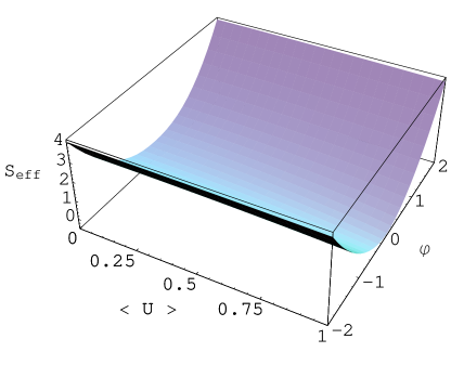
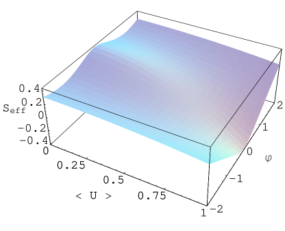
Figure 6: The effective action is plotted for $T<T_{c}$ on the left and $T>T_{c}$ on the right, as a function of $\varphi$ and the Polyakov loop $\langle U\rangle$ for $SU(2)$ gauge group.

The $SU(2)$ theory has a critical temperature

$$T_{c}=\sqrt{2\over\lambda}R^{-1}.$$ (72)

For temperatures in the range $R^{-1}\ll T<T_{c}$, there is a saddle point at $\langle U\rangle=\varphi=0$ with one unstable direction along the $U$-axis. This saddle point is actually stable below the Hagedorn or deconfinement temperature on ${S}^{3}$ [7] and is the confined phase with zero expectation value for the Polyakov loop.

The situation changes beyond the critical temperature $T_{c}$ when a second unstable direction appears at $\langle U\rangle=0$. The full effective potential (60) now exhibits new extrema or saddle points with

$$\left({\varphi_{a1}\over T}\right)^{2}\neq 0$$ (73)

as in Figure 6. It is easy to see that these saddle points must exist. At $\langle U\rangle=0$, we have seen that there is an instability at $\varphi_{1}=0$. For large values of $\varphi_{1}$, the quadratic term in (60) dominates since ${\cal H}(\varphi)$ vanishes exponentially. Hence there must be a point for intermediate values of $(\varphi_{1}/T)$ which is stable to fluctuations along this direction. Importantly, in Figure 6 we see that these points are unstable to rolling to the $\langle U\rangle=1$ vacuum. Hence these new extrema are indeed saddle points. The instability to fluctuations in $\varphi$ around $\varphi=0$ persists for a finite range of values of the Polyakov loop $\langle U\rangle$. At very high temperatures above $T_{c}$, all points with $\varphi=0$ and $0\leq\langle U\rangle\leq{1\over\sqrt{2}}$ acquire an unstable mode along the $\varphi$ axis.

$SU(N)$ at large $N$

The above picture generalizes rather directly for $SU(N)$ gauge group. The unstable extremum at $\varphi_{ai}=0$ is characterized by a uniform distribution of the eigenvalues of the Polyakov loop,

$$\theta_{j}={2\pi\over N}j+c(N)\;,\qquad j=1,2,\ldots N$$ (74)

where $c$ is a constant chosen so that

$$\sum_{i=1}^{N}\theta_{i}=\;0\;{\rm mod}\;2\pi.$$ (75)

It is a stable ground state of the theory below the Hagedorn temperature on ${S}^{3}$ [7] and leads to a vanishing Polyakov loop and infinite free energy for colored sources. At strong coupling (and large $N$) and below the deconfinement transition, this phase is dual to the thermal AdS space saddle point of semiclassical Euclidean gravity.

The temperatures we are considering, $T\gtrsim(\sqrt{\lambda}R)^{-1}$ at weak coupling are far above the deconfinement transition and hence $\langle U\rangle=0$ is only an unstable extremum. The question we are interested in is, whether there are new unstable directions about this saddle point. This may be answered by examining the quadratic form in $\varphi$ (68). The associated matrix is a circulant, whose eigenvalues may be determined relatively easily (see Appendix A). In the large $N$ limit, we find that as the temperature is increased beyond a critical value new unstable directions start to appear, with the first negative eigenvalue occurring at the critical temperature

$$T_{c}={\pi\over\sqrt{2\lambda}}\;R^{-1}.$$ (76)

As the temperature is increased beyond this, we find more negative modes, each one appearing when the temperature hits the critical values (Appendix A),

$$T_{c}^{(l)}=(2l-1){\pi\over\sqrt{2\lambda}}R^{-1},\qquad l=1,2,\ldots.$$ (77)

The number of unstable directions is $(N/2-1)$ when $N$ is even and $(N-1)/2$ for $N$ odd, and hence is formally infinite in the large $N$ limit in the one loop approximation. Interestingly, this is consistent with what is observed for the small AdS black hole in classical gravity [17]. We should however, bear in mind that in weakly coupled field theory we expect perturbation theory for the constant modes or low lying harmonics on $S^{3}$ to break down at high enough temperatures where the size of the three sphere approaches the non-perturbative magnetic screening length $R\sim(\lambda T)^{-1}$. Therefore we can trust (77) for $(2l-1)\ll{1\over\sqrt{\lambda}}$. We also point out that the modes that we see becoming unstable are constant on $S^{3}\times S^{1}$, the higher Kaluza-Klein harmonics remain massive at these temperatures and within the regime of validity of the one loop approximation.

As in the $SU(2)$ example we then find new extrema where

$$\sum_{a=1}^{6}\varphi_{ai}^{2}\neq 0\,.$$ (78)

The existence of these saddle points follows from the instabilities at $\varphi=0$ and the fact that at large $\varphi$ the quadratic mass term dominates the potential. This can be verified by numerically plotting the full expression for the potential (60). Our potential is written in terms of the $SO(6)$-invariant radial coordinate $\sum_{a}{\varphi_{ai}^{2}}$ in the space of the six scalars. In a non-compact space, a non-zero value for this coordinate at the new saddle points would be interpreted as breaking the global R-symmetry of the ${\cal N}=4$ theory to $SO(5)$

$$SO(6)\longrightarrow SO(5).$$ (79)

How can we understand this in the context of the field theory on a compact space, namely the three-sphere, where we do not expect to see symmetry breaking.



 Symmetry breaking at large N

Symmetry breaking is not normally possible in a finite volume since the wave function spreads over the vacuum manifold or points in field space which are related by the symmetry. This means that we must average over the orbit of the symmetry group, or include in the partition function, an integral over such states. Concretely, introducing the notation

$$\rho_{i}=\left(\sum_{a=1}^{6}\varphi_{ai}^{2}\right)^{1\over 2}\,\qquad i=1,2,\ldots N$$ (80)

for the radial mode of scalar eigenvalues, if $\rho_{i}$ is allowed a non-vanishing value, then we must integrate over the corresponding orbit $SO(6)/SO(5)\simeq S^{5}$. Formally then, we must write the partition function as

$$Z=\int\prod_{j=1}^{N}(d\rho_{j}\;\rho_{j}^{5})\;(d\Omega_{5})^{N}\;e^{-S_{\rm eff}[{\rho_{i}}]}.$$ (81)

Actually the above is not completely correct since the orbit of the global symmetry group is the symmetric product space, ${\rm Sym}_{N}(SO(6)/SO(5))\simeq{\rm Sym}_{N}(S^{5})$, due to the action of the Weyl subgroup of $SU(N)$. However, what is important for us is that the space is $5N$-dimensional and the full partition function is

$$Z\sim\int\prod_{j=1}^{N}(d\rho_{j})\;e^{-S_{\rm eff}[{\rho_{i}}]+5\sum_{i=1}^{N}\ln\;\rho_{i}}.$$ (82)

However $S_{\rm eff}$ scales as $N^{2}$ in the large $N$ limit while the measure from averaging over the orbit of the symmetry group is of ${\cal O}(N^{1})$. Hence, in the large $N$ limit we may neglect the contribution from the latter to compute the saddle points of the effective action. Note that taking the volume of the space to infinity would also have a similar effect since $S_{\rm eff}$ scales extensively with the volume of the three-sphere.

Symmetry breaking may now be defined in the large $N$ theory in the conventional way. At finite $N$ we introduce a source which breaks the $SO(6)$ symmetry,

$$\delta S=N^{2}\epsilon_{i}\;\varphi_{ai}.$$ (83)

Taking $N$ to infinity first, followed by $\epsilon$ to zero permits breaking of the $SO(6)$ symmetry.

As in the $SU(2)$ example, the unstable directions persist as we move away from $\langle U\rangle=0$, the uniform distribution for the $\theta_{i}$. Indeed, as some of the $\theta_{i}$ start to clump together, the cosines in (68) cease to be negative and some of the negative modes start disappearing. This is true in particular when the distribution develops a gap, an extreme example of which is the delta function distribution associated to the big AdS black hole which is the global minimum of the action.

3.3.3 The gravity interpretation

We now compare and contrast the weak coupling, high temperature picture obtained above of large $N$, ${\cal N}=4$ SYM on ${S}^{3}\times{S}^{1}$ with the known strongly coupled dual, namely gravity/string theory on ${\rm AdS}_{5}\times{S}^{5}$.

The free ${\cal N}=4$ theory on ${S}^{3}$ analyzed in [7] exhibits two different phases at large $N$, a confined phase and a deconfined phase separated by a first order phase transition at $T=T_{H}=1/(R\ln(7-4\sqrt{3})^{-1})$. It is believed that these two phases at $\lambda=0$ are the infinitely curved, stringy versions of thermal AdS space and the big AdS Schwarzschild black hole which are separated by a first order Hawking-Page transition.

In the free ($\lambda=0$) Yang-Mills theory, above $T_{H}$ the thermal AdS extremum is unstable. Our field theory results above show that the weakly interacting large $N$ field theory develops additional (unstable) saddle points above a critical temperature

$$T_{c}={\pi\over\sqrt{2\lambda}}\;R^{-1}.$$ (84)

These configurations with scalar expectation values only preserve an $SO(5)$ subgroup of the $SO(6)$ R-symmetry of ${\cal N}=4$ theory. We stress that these saddle points are not themselves stable, but have lower actions than the “thermal AdS” configuration (characterized by $\langle U\rangle=\varphi_{ia}=0$) which develops unstable directions towards these new saddle points at high temperature.

We interpret these new unstable directions as the infinite curvature or string scale manifestations of the Gregory-Laflamme instability of the small AdS Schwarzschild black hole, a phenomenon which is observed at weak curvature or strong ’t Hooft coupling ($\lambda\rightarrow\infty$). As described in section 2, in semiclassical gravity this instability is a dynamical instability at the small AdS black hole saddle point which is already thermodynamically unstable. The dynamical instability triggers the localization of the small black hole on the $S^{5}$ breaking the $SO(6)$ isometry to $SO(5)$.

There is of course a crucial distinction between the weak and strong coupling regimes. The dynamical instability we see occurs at temperatures $T\gtrsim O(R^{-1}/\sqrt{\lambda})$ which is far above the Hagedorn temperature. At these temperatures the saddle point corresponding to the small black hole has already disappeared [7] or merged with the thermal AdS configuration [9]. Hence it is the $\langle U\rangle=0$ extremum, associated to thermal AdS at strong coupling, which becomes “unstable to localization on ${S}^{5}$”.

It is easy to see how the the strong and weak coupling pictures might match on smoothly. As the ’t Hooft coupling is increased, the critical temperature (76) decreases at weak coupling. It is conceivable that as we move towards strong coupling the critical temperature $T_{c}$ at which the new instabilities are triggered, eventually becomes comparable to and lower than the Hagedorn temperature where the small black hole exists as a saddle point of the action. Hence for temperatures in the range $T_{c}<T<T_{H}$, the small black hole saddle point can be expected to be unstable to new saddle points which break the $SO(6)_{R}$ down to $SO(5)_{R}$. As we have already mentioned in the introduction, there is also the possibility that at relatively small ’t Hooft couplings with dual gravity curvatures approaching the string scale, the small black hole likely makes a transition to a highly excited state of strings before any Gregory-Laflamme like instabilities can kick in.

4 Summary and conclusions

In this paper we have performed an explicit computation of a joint one loop effective action for the eigenvalues of constant scalar fields and the Polyakov loop in $SU(N)$ ${\cal N}=4$ SYM on ${S}^{3}\times{S}^{1}$. Our perturbative computation is valid for temperatures $0\leq T\ll{1\over\lambda}R^{-1}$ and in particular for temperatures where the size of the three sphere approaches the Debye screening length of the Yang-Mills plasma $R\sim(\sqrt{\lambda}T)^{-1}$.

We find at large $N$, above a critical temperature

$$T_{c}={\pi\over\sqrt{2\lambda}}\;R^{-1}$$ (85)

the effective potential exhibits new extrema with non-zero values for the ${\cal N}=4$ scalar fields. The emergence of these saddle points is accompanied by new unstable directions at the thermal AdS extremum which was characterized by a uniform distribution of Polyakov loop eigenvalues. The latter is already unstable at temperatures below $T_{c}$ but new instabilities along the scalar directions appear at $T_{c}$. We believe these unstable directions to be the small ’t Hooft coupling manifestations of a well known dynamical instability in the gravity dual of the strongly coupled gauge theory – the Gregory-Laflamme localization instability of the small black hole in ${\rm AdS}_{5}\times{S}^{5}$. Note that the weak coupling instability we have found is not associated to a small black hole saddle point since the latter does not exist at $T_{c}$ or has merged with the thermal AdS saddle point at the Hagedorn temperature far below $T_{c}$.

Many open questions remain, chief among these being the physical meaning of the instabilities of the thermal AdS saddle point at these high temperatures, and how they turn into dynamical instabilities of the small black hole at intermediate or strong coupling. Possible answers to this question have been presented in the paper and are summarized in a phase plot in Figure 1.

We also find that whenever the temperature reaches a critical value $T_{c}^{(l)}=(2l-1)T_{c}$ for $l=1,2,3,\ldots$ a new negative mode shows up. A similar infinite set of negative modes is also expected from the classical gravity analysis of [17]. It would be interesting to understand the similarities between the two pictures better, particularly whether the linear dependence of $T_{c}^{(l)}$ on $l$ can be understood at all from the gravity perspective, even though the latter is only valid at strong ’t Hooft coupling. It is somewhat tantalizing that the values of $T_{c}^{(l)}$ for the first five negative modes obtained numerically in [17] appear to exhibit this linear behaviour.

A natural extension of the results of this paper is to include a finite chemical potential for an $SO(2)$ subgroup of the $SO(6)$ R-symmetry. The corresponding gravity dual involves charged black holes. These also exhibit Gregory-Laflamme instabilities and we explore them at weak coupling in the holographic dual in [28]. The weak coupling analysis appears to exhibit stable saddle points with global symmetry breaking at finite chemical potential. The phase structure for R-charged black holes was discussed in [29, 30, 31] and the dual field theory phase diagram at weak coupling has been explored recently in [11].

The effective potential we have computed is a static effective potential since we calculate it in the Euclidean theory on ${S}^{3}\times{S}^{1}$. It is difficult to interpret it as an effective potential in the Lorentzian field theory on ${S}^{3}\times{\mathbb{R}}$ since it is not clear what the Polyakov loops mean in the Lorentzian theory. However, there is a different analytic continuation to Lorentzian signatures where our effective potential may be usefully interpreted. This involves analytically continuing one of the angular directions on the three-sphere to Lorentzian signature which maps ${S}^{3}\times{S}^{1}$ to ${\rm dS}_{3}\times{S}^{1}$, leaving the thermal circle as a spatial circle. As discussed originally in [32] this is the boundary of a “topological black hole” constructed as a certain orbifold of ${\rm AdS}_{5}$ [33] . The topological black hole decays to an AdS bubble of nothing [34] where the bounce solution is the Euclidean small AdS black hole which is unstable to localization on the ${S}^{5}$. As pointed out by the authors of [32], this should be described in a dual field theory via an effective potential that allows rolling in a direction breaking the $SO(6)$ symmetry. The methods presented in our paper and our effective potential naturally allow such a holographic description of the process of gravitational decay via the bubble of nothing, at least in an adiabatic approximation.

Acknowledgments

We would like to thank Gert Aarts, Sean Hartnoll and Shiraz Minwalla for enjoyable discussions and very useful comments. SPK and AN are supported by PPARC Advanced Fellowships.

Appendix A: Unstable directions of the effective potential

In this appendix, we perform the small fluctuation analysis of the effective potential expanded about $\varphi\approx 0$ for a uniformly distributed configuration of Polyakov loop eigenvalues (68). This will tell us about instabilities around the thermal AdS saddle point as a function of temperature.

We are interested in the eigenvalues of the quadratic form in $\tilde{\varphi_{i}}\tilde{\varphi_{j}}$ appearing in (68) which can be rewritten as (neglecting overall multiplicative constants)

$$\begin{split}\sum_{ij=1}^{N}\tilde{\varphi_{i}}\tilde{\varphi_{j}}\Big{(}&\delta_{ij}\left[{R^{-2}\over\lambda T^{2}}\;(N-1)-{1\over 2}+{1\over 2N}\delta_{N,{\rm odd}}\right]-\\ &(1-\delta_{ij})\left[{R^{-2}\over\lambda T^{2}}+{4\over\pi^{2}}\sum_{k=1}^{\infty}{1\over(2k-1)^{2}}\cos\left({2\pi\over N}(2k-1)(i-j)\right)\right]\Big{)},\end{split}$$ (86)

where we have used $\theta_{ij}=2\pi(i-j)/N$ at the thermal AdS saddle point.

The quadratic form above is an example of an $N\times N$ circulant matrix i.e. a matrix each of whose rows (or columns) can be obtained by cyclic permutations of the elements of one particular row (or column). The $N$ eigenvalues of a circulant matrix with a row of the form $(x_{1},x_{2},\ldots x_{N})$ are given by

$$\lambda_{\ell}=\sum_{m=1}^{N}x_{m}\;e^{{2\pi i\over N}(m-1)\ell}\qquad\ell=0,1,2,\ldots N-1.$$ (87)

Applying this formula to the quadratic form (86), we can find the eigenvalues easily. The expressions simplify at large $N$ and we quote the results below

$$\begin{split}&\lambda_{0}=0\\ \\ &\lambda_{2\ell-1}=N\left[\left({R^{-2}\over\lambda T^{2}}\right)-{2\over\pi^{2}}{1\over(2\ell-1)^{2}}+O\left({1\over N^{2}}\right)\right]\\ \\ &\lambda_{2\ell}=N\left[\left({R^{-2}\over\lambda T^{2}}\right)+O({1\over N^{2}})\right]\end{split}$$ (88)

with $\ell=1,2,\ldots$.

It is clear that each of the eigenvalues with odd labels becomes negative at a critical temperature

$$T_{\ell}={(2\ell-1)\pi\over\sqrt{2\lambda}}R^{-1}.$$ (89)

and the first instability occurs at

$$T_{c}={\pi\over\sqrt{2\lambda}}R^{-1}.$$ (90)

References

- [1]
- [2] J. M. Maldacena, “The large N limit of superconformal field theories and supergravity,” Adv. Theor. Math. Phys. 2, 231 (1998) [Int. J. Theor. Phys. 38, 1113 (1999)] [arXiv:hep-th/9711200].
- [3] E. Witten, “Anti-de Sitter space and holography,” Adv. Theor. Math. Phys. 2, 253 (1998) [arXiv:hep-th/9802150].
- [4] E. Witten, “Anti-de Sitter space, thermal phase transition, and confinement in gauge theories,” Adv. Theor. Math. Phys. 2, 505 (1998) [arXiv:hep-th/9803131].
- [5] O. Aharony, S. S. Gubser, J. M. Maldacena, H. Ooguri and Y. Oz, “Large N field theories, string theory and gravity,” Phys. Rept. 323, 183 (2000) [arXiv:hep-th/9905111].
- [6] B. Sundborg, “The Hagedorn transition, deconfinement and N = 4 SYM theory,” Nucl. Phys. B 573, 349 (2000) [arXiv:hep-th/9908001].
- [7] O. Aharony, J. Marsano, S. Minwalla, K. Papadodimas and M. Van Raamsdonk, “The Hagedorn / deconfinement phase transition in weakly coupled large N gauge theories,” Adv. Theor. Math. Phys. 8 (2004) 603 [arXiv:hep-th/0310285].
- [8] O. Aharony, J. Marsano, S. Minwalla, K. Papadodimas and M. Van Raamsdonk, “A first order deconfinement transition in large N Yang-Mills theory on a small ,” Phys. Rev. D 71, 125018 (2005) [arXiv:hep-th/0502149].
- [9] L. Alvarez-Gaume, C. Gomez, H. Liu and S. Wadia, “Finite temperature effective action, AdS(5) black holes, and 1/N expansion,” Phys. Rev. D 71, 124023 (2005) [arXiv:hep-th/0502227].
- [10] S. W. Hawking and D. N. Page, “Thermodynamics Of Black Holes In Anti-De Sitter Space,” Commun. Math. Phys. 87, 577 (1983).
- [11] D. Yamada and L. G. Yaffe, “Phase diagram of N = 4 super-Yang-Mills theory with R-symmetry chemical potentials,” arXiv:hep-th/0602074.
- [12] T. Harmark and M. Orselli, “Quantum mechanical sectors in thermal N = 4 super Yang-Mills on R x S**3,” arXiv:hep-th/0605234.
- [13] R. Gregory and R. Laflamme, “Black strings and p-branes are unstable,” Phys. Rev. Lett. 70, 2837 (1993) [arXiv:hep-th/9301052].
- [14] S. S. Gubser and I. Mitra, “Instability of charged black holes in anti-de Sitter space,” arXiv:hep-th/0009126.
- [15] S. S. Gubser and I. Mitra, “The evolution of unstable black holes in anti-de Sitter space,” JHEP 0108, 018 (2001) [arXiv:hep-th/0011127].
- [16] H. S. Reall, “Classical and thermodynamic stability of black branes,” Phys. Rev. D 64, 044005 (2001) [arXiv:hep-th/0104071].
- [17] V. E. Hubeny and M. Rangamani, “Unstable horizons,” JHEP 0205, 027 (2002) [arXiv:hep-th/0202189].
- [18] O. Aharony, J. Marsano, S. Minwalla and T. Wiseman, “Black hole - black string phase transitions in thermal 1+1 dimensional supersymmetric Yang-Mills theory on a circle,” Class. Quant. Grav. 21, 5169 (2004) [arXiv:hep-th/0406210].
- [19] G. T. Horowitz and J. Polchinski, “A correspondence principle for black holes and strings,” Phys. Rev. D 55, 6189 (1997) [arXiv:hep-th/9612146].
- [20] L. Alvarez-Gaume, P. Basu, M. Marino and S. R. Wadia, “Blackhole / string transition for the small Schwarzschild blackhole of and critical unitary matrix models,” arXiv:hep-th/0605041.
- [21] J. P. Gregory and S. F. Ross, “Stability and the negative mode for Schwarzschild in a finite cavity,” Phys. Rev. D 64, 124006 (2001) [arXiv:hep-th/0106220].
- [22] J. de Boer, L. Maoz and A. Naqvi, “Some aspects of the AdS/CFT correspondence,” arXiv:hep-th/0407212.
- [23] E. Elizalde and A. C. Tort, “A note on the Casimir energy of a massive scalar field in positive curvature space,” Mod. Phys. Lett. A 19 (2004) 111 [arXiv:hep-th/0306049].
- [24] R. M. Cavalcanti, C. Farina and F. A. Barone, “Radiative corrections to Casimir effect in the lambda model,” arXiv:hep-th/0604200.
- [25] J. I. Kapusta, Finite-temperature field theory, (Cambridge University Press, Cambridge, 1989)
- [26] M. Le Bellac, Thermal field theory, (Cambridge University Press, Cambridge, 1996).
- [27] R. Narayanan and H. Neuberger, “Chiral symmetry breaking at large N(c),” Nucl. Phys. B 696, 107 (2004) [arXiv:hep-lat/0405025].
- [28] T. Hollowood, S. P. Kumar and A. Naqvi, to appear.
- [29] A. Chamblin, R. Emparan, C. V. Johnson and R. C. Myers, “Charged AdS black holes and catastrophic holography,” Phys. Rev. D 60, 064018 (1999) [arXiv:hep-th/9902170].
- [30] M. Cvetic and S. S. Gubser, “Phases of R-charged black holes, spinning branes and strongly coupled gauge theories,” JHEP 9904, 024 (1999) [arXiv:hep-th/9902195].
- [31] P. Basu and S. R. Wadia, “R-charged AdS(5) black holes and large N unitary matrix models,” Phys. Rev. D 73, 045022 (2006) [arXiv:hep-th/0506203].
- [32] V. Balasubramanian, K. Larjo and J. Simon, “Much ado about nothing,” Class. Quant. Grav. 22, 4149 (2005) [arXiv:hep-th/0502111].
- [33] M. Banados, A. Gomberoff and C. Martinez, “Anti-de Sitter space and black holes,” Class. Quant. Grav. 15, 3575 (1998) [arXiv:hep-th/9805087].
- [34] V. Balasubramanian and S. F. Ross, “The dual of nothing,” Phys. Rev. D 66, 086002 (2002) [arXiv:hep-th/0205290].
- [35]