Predictions of Dynamically Emerging Brane Inflation Models

Abstract

We confront the recent proposal of Emerging Brane Inflation with WMAP3+SDSS, finding a scalar spectral index of $n_{s}=0.9659^{+0.0049}_{-0.0052}$ in excellent agreement with observations. The proposal incorporates a preceding phase of isotropic, non accelerated expansion in all dimensions, providing suitable initial conditions for inflation. Additional observational constraints on the parameters of the model provide an estimate of the string scale.

A graceful exit to inflation and stabilization of extra dimensions is achieved via a string gas. The resulting pre-heating phase shows some novel features due to a redshifting potential, comparable to effects due to the expansion of the universe itself. However, the model at hand suffers from either a potential over-production of relics after inflation or insufficient stabilization at late times.

I Introduction

Inflation provides a natural explanation for major problems of standard cosmology such as the homogeneity, horizon and flatness problems Guth . An almost scale-invariant spectrum of adiabatic cosmological fluctuations was predicted Lukash ; ChibMukh more than a decade before the cosmic microwave background anisotropies were analyzed  WMAP ; Maxima ; Boomerang ; COBE . Encouraged by the great success of the inflationary paradigm, one is urged to find a successful realization of inflation within more fundamental theories, such as string theory.

The heuristic approach of obtaining inflation consists of introducing one or more scalar fields (inflatons), which evolve slowly due to some appropriately tuned potential. Simple single field models require the inflaton to start out at a value larger than the Planck mass. However, at these values radiative corrections to the inflaton mass threaten to spoil slow roll dynamics. Therefore, unless some underlying symmetry protects the inflaton mass, it is hard to implement an inflationary scenario within gauge theories. Moreover, in the framework of four dimensional inflationary models the physical interpretation of the inflaton is unclear. Generally, it is taken to be a singlet of the Standard Model and typically of all of the visible sector too. (See Allahverdi:2006iq for a recently proposed exception.)

The advent of extra dimensions ADD ; RS opened up a venue for new inflationary scenarios where the inflaton has a physical meaning; for example, in brane-antibrane inflationary models the inter-brane separation serves as the inflaton DT ; Shafi . However, to provide a sufficient amount of inflation in brane-antibrane models, one requires fine tuning of initial conditions Cliff ; Cliff2 , e.g. large inter brane separation, special configurations or very weak couplings.

In this article, we would like to discuss the recent proposal of emerging brane inflation size ; Shuhmaher:2005pw that makes use of extra dimensions, a gas of p-branes in the bulk to drive an initial isotropic but non accelerated expansion of the universe, as well as orbifold fixed planes responsible for contraction of the extra dimensions and inflation of our three dimensions. The presence of a string gas at the end of inflation provides a graceful exit, pre-heating and stabilization of extra dimensions. The model at hand does not need any fine tuning of initial conditions and will turn out to be in good agreement with observations.

In this scenario the multidimensional universe starts out small and hot, with our three dimensions compactified on a torus and the extra dimensions on an orbifold of the same size. The pre-inflationary expansion size ; Shuhmaher:2005pw is governed by topological defects (p-branes) in the bulk and responsible for a large inter brane separation. As the universe expands isotropically due to the gas of p-branes, the energy density stored in the gas gets diluted until additional weak forces come into play, changing the overall dynamics. For example, branes pinned to orbifold fixed planes, which exhibit an attractive force, may eventually cause a contraction of the extra dimensions while our dimensions inflate. From the four dimensional point of view, the inflaton is identified with the radion and consequently, the pre-inflationary bulk expansion explains the large initial value of the inflaton. Inflation comes to an end when the extra dimensions shrink down to a small scale where moduli trapping Watson:2003gf ; Patil:2004zp ; Kofman:2004yc ; Watson:2004aq and pre-heating Traschen:1990sw ; Shtanov:1994ce ; Kofman:1994rk ; Kofman:1997yn ; Greene:1997fu ; Felder:2000hj can occur.

Our main goal in this article is to examine the viability of the emerging brane inflation model outlined above and to make contact with observations.

The outline of this article is as follows: In Ch. II we review the details of the model, followed by a computation (Ch. III) within the slow roll approximation of the spectral index $n_{s}$, the running of the index $d\,n_{s}/(d\,\ln k)$, the scalar to tensor ratio $r$ and the tensor index $n_{T}$. We confront our predictions with the observation of the cosmic microwave background radiation measured by the Wilkinson Microwave Anisotropy Probe (WMAP3) Spergel:2006hy ; Page:2006hz ; Hinshaw:2006ia ; Jarosik:2006ib and the Sloan Digital Sky Survey (SDSS) Tegmark:2001jh , resulting in good agreement. In order to get sufficient initial expansion one requires the inter brane potential to remain subdominant for a long time compared to the energy density stored in the bulk p-branes. This requirement imposes constraints on the scale of interactions between branes pinned to the orbifold fixed points. This, together with constraints from observational data, will be sufficient to provide an estimate of the string scale. In Chapter IV, we study the viability of pre-heating after inflation and stabilization at late times. While pre-heating can occur in the standard manner, albeit some novel effects are present, we do find potential problems associated with either late time stabilization or relics: if the branes pinned to the orbifold fixed planes annihilate after inflation they could produce an over-abundance of relics such as cosmic strings, and if they do not annihilate they will destabilize the extra dimensions at late times. We conclude with a comment on open issues within the framework of emerging brane inflation.

II The Model

Following Shuhmaher:2005pw , we assume a spacetime

$${\cal M}={\cal R}\times T^{3}\times T^{d}/Z_{2}\,,$$ (1)

so that our three dimensions have the topology of a torus $T^{3}$, and the $d$ extra dimensions are compactified on the orbifold $T^{d}/Z_{2}$. Note, that this specific choice of the manifold is not crucial for the model – many other manifolds distinguishing our three dimensions could be chosen instead. Next, we assume that pairs of branes are pinned to the different orbifold fixed planes a distance $r$ apart. Furthermore, we also assume inter brane interactions such that a weak attractive force is generated via some potential $V$. It should be noted that we take a phenomenological approach and postulate the existence of a potential with the desired properties. A discussion of possible origins of inter-brane potentials can be found in DT .

The special feature of the underlying scenario is the pre-inflationary dynamics which explains the large size of the extra dimensions just before inflation. Initially, the universe starts out small and hot with all spatial dimensions of the same size. The bulk is filled with a gas of p-branes. In this phase, the energy density in the brane gas is assumed to be many orders of magnitude larger than the potential energy density, which provides the force between the orbifold fixed planes. Thus, the universe expands isotropically but not inflationary, as shown in size . During the expansion phase the bulk energy density of the gas decreases and eventually the potential $V$ begins to dominate, causing inflation of the directions parallel to the orbifold fixed planes, and contraction of the extra dimensions. It should be noted that whether or not inflation occurs is sensitive to the form of the inter-brane potential $V$.

Following Shuhmaher:2005pw , we consider a potential of the form

$$V(r)=-\mu{1\over r^{n}}\,,$$ (2)

where $r$ is the inter brane separation and $n>0$ is a free parameter, which could in principle be computed from the underlying fundamental theory. As we shall see below, this form of the potential results in inflation.

We shall first compute how dynamics can be described in a four dimensional effective theory. Let $G_{ab}$ be the metric for the full space-time with coordinates $X^{a}$. In the absence of spatial curvature, the metric of a maximally symmetric space which distinguishes ’our’ three dimensions is given by

$$ds^{2}=G_{ab}dX^{a}dX^{b}\,=\,d{t^{\prime}}^{2}-\alpha(t^{\prime})^{2}d{\bf x}^{2}-b(t^{\prime})^{2}d{\bf y}^{2}\,,$$ (3)

where ${\bf x}$ denotes the three coordinates parallel to the orbifold fixed planes and ${\bf y}$ denotes the coordinates of the $d$ perpendicular directions.

Our goal is to find a four-dimensional effective potential which governs the inflationary phase. We start out with the higher dimensional action

$$S=\int d^{d+4}X\sqrt{-\det G_{ab}}\left\{\frac{1}{16\pi G_{d+4}}R_{d+4}+\hat{\cal L}_{M}\right\}\,,$$ (4)

where $R_{d+4}$ is the $d+4$ dimensional Ricci scalar and $\hat{\cal L}_{M}$ is the matter Lagrangian density with the metric determinant factored out. Note that the dilaton is assumed to be fixed already, e.g. via the proposal of Cremonini:2006sx . In the effective four-dimensional action, the radion $b(t)$ is replaced by a canonically normalized scalar field $\varphi(t)$ which is related to $b(t)$ through Battefeld:2005av ; Carroll:2001ih

$$\varphi=\beta^{-1}m_{pl}\ln(b)\,,$$ (5)

where

$$m^{2}_{pl}=\frac{1}{8\pi G_{4}}$$ (6)

is the reduced four dimensional Planck mass and we defined

$$\beta^{-1}:={\sqrt{d(d+2)\over 2}}\,.$$ (7)

After performing a dimensional reduction and a conformal transformation to arrive at the Einstein frame Battefeld:2005av ; Carroll:2001ih we are left with

$$S=\int d^{4}xa^{3}\left\{\frac{1}{2}m_{pl}R_{4}\right. - \left.\frac{1}{2}(\partial\varphi)^{2}\right.$$

$$+ \left.{\cal V}e^{-d\varphi/m_{pl}\beta}\hat{\cal L}_{M}\right\}\,,$$

where

$${\cal V}\,=\,\int d^{d}{\bf y}\,=\,l^{d}_{s}$$ (9)

is the volume of the extra dimensions, and

$$ds_{E}^{2} = b^{d}(dt^{\prime 2}-\alpha^{2}d{\bf x}^{2})$$ (10)

$$= dt^{2}-a(t)^{2}d{\bf x}^{2}$$

is the effective four dimension metric. Further, assuming that the initial separation between the orbifold fixed planes is of string length $l_{s}$ one can compute the distance between the orbifold fixed planes to

$$r(t^{\prime})=l_{s}b(t^{\prime})\,.$$ (11)

Note that $b=1$ corresponds to the string scale. Setting $\hat{\mathcal{L}}_{M}=V$ yields

$$V_{4d}(\varphi)\, = \,g^{4}_{s}l^{d}_{s}b(\varphi)^{-d}V(r(\varphi))$$ (12)

$$= -\mu g^{4}_{s}l^{d-n}_{s}e^{-\tilde{\alpha}{\varphi\over{m_{pl}}}}\,,$$

where we used (2), restored the string coupling dependence and defined

$${\tilde{\alpha}}:=(n+d)\beta\,.$$ (13)

To account for the brane tension/zero cosmological constant today we add a positive constant $V_{0}$ to the effective potential (12) and arrive at the effective four dimensional potential

$$V_{eff}(\varphi) = V_{0}-\mu g^{4}_{s}l^{d-n}_{s}e^{-\tilde{\alpha}{\varphi\over{m_{pl}}}}$$ (14)

$$= V_{0}(1-\zeta e^{-\tilde{\alpha}/m_{p}\,\varphi})$$

where we defined

$$\zeta:={\mu g^{4}_{s}l^{d-n}_{s}\over V_{0}}\,.$$ (15)

This potential yields inflation for large enough values of the radion/inflaton $\varphi$. Similar potentials have been considered before, see e.g. Conlon:2005jm in the context of brane inflation or Stewart:1994ts in the context of supergravity. These proposals differ from ours in the form of the graceful exit, the details of pre-heating as well as the the pre-inflationary dynamics of our model, which pull $\varphi$ far from its minimum such as to provide suitable initial conditions for inflation without fine tuning.

III Predictions

Inflation gives rise to a viable mechanism of structure formation: quantum vacuum fluctuations, present during inflation on microscopic scales, exit the Hubble radius and are subsequently squeezed, resulting in classical perturbations at late times, see e.g. Mukhanov:1990me . Moreover, current observations are precise enough to distinguish between different inflationary models Spergel:2006hy ; Page:2006hz ; Hinshaw:2006ia ; Jarosik:2006ib ; Tegmark:2001jh ; Kinney:2006qm ; Martin:2006rs .

In the following, we derive observable quantities within the slow roll approximation and make contact with observations. Thereafter, we show how one can estimate the string scale in the model at hand.

III.1 Cosmological Parameters

The equation of motion for a scalar field in an expanding universe is given by

$${\ddot{\varphi}}+3H\dot{\varphi}+V_{I}^{\prime}=0\,,$$ (16)

where $H=\dot{a}/a$ is the Hubble parameter, $V_{I}:=V_{eff}$ from (14) is the inflaton potential and $V_{I}^{\prime}:=dV_{I}/d\phi$. If the scalar field $\varphi$ governs the evolution of the Universe, the Friedmann Robertson Walker equations become

$$H^{2} = \frac{1}{3m^{2}_{pl}}\left[\frac{1}{2}{\dot{\varphi}}^{2}+V_{I}(\varphi)\right]\,,$$ (17)

$$\left(\frac{\ddot{a}}{a}\right) = \frac{1}{3m^{2}_{pl}}\left[V_{I}(\varphi)-{\dot{\varphi}}^{2}\right]\,.$$ (18)

If the potential energy of the inflaton dominates over the kinetic energy, accelerated expansion of the universe results. In other words, if the potential is flat enough to allow for slow roll of the inflaton field, inflation occurs. In this case (16) and (17) become

$$3H\dot{\varphi} = -V_{I}^{\prime}\,,$$ (19)

$$H^{2} = \frac{V_{I}}{3m^{2}_{pl}}\,,$$ (20)

where we assumed ${\dot{\varphi}}^{2}\ll V_{I}$ and ${\ddot{\varphi}}\ll 3H\dot{\varphi}$.

This approximation is valid if both the slope and the curvature of the potential are small, that is if the slow roll parameters

$$\varepsilon = \frac{m^{2}_{pl}}{2}\left(\frac{V_{I}^{\prime}}{V_{I}}\right)^{2}\,,$$ (21)

$$\eta = m^{2}_{pl}\frac{V_{I}^{\prime\prime}}{V}\,.$$ (22)

satisfy $\varepsilon\ll 1$ and $\eta\ll 1$. Let $\varphi_{i}$ denote the value of the inflaton field N e-folds before the end of inflation. This value can be determined from

$$N = \int^{t_{f}}_{t_{i}}H(t)dt$$ (23)

$$\approx \frac{1}{m^{2}_{pl}}\int^{\varphi_{i}}_{\varphi_{f}}\frac{V}{V^{\prime}}d\varphi\,,$$

where $\varphi_{f}$ is the value of the inflaton field at which the slow roll approximation breaks down.

Within the slow roll regime one can then compute the scalar spectral index, the scalar to tensor ratio and the tensor spectral index to Kinney:2006qm

$$n_{s} \approx 1-6\varepsilon+2\eta\,,$$ (24)

$$r \approx 16\epsilon\,,$$ (25)

$$n_{T} \approx -r/8\,,$$ (26)

where $\epsilon$ and $\eta$ have to be evaluated at $\varphi_{i}$. For the potential (14) the slow roll parameters become

$$\varepsilon = \frac{\tilde{\alpha}^{2}}{2}\frac{1}{(\zeta^{-1}e^{\tilde{\alpha}/m_{pl}\,\varphi}-1)^{2}}\,,$$ (27)

$$\eta = -\tilde{\alpha}^{2}\frac{1}{\zeta^{-1}e^{\tilde{\alpha}/m_{p}\,\varphi}-1}\,.$$ (28)

Since $|\eta|>\varepsilon$ in our case, inflation ends once $|\eta|=\mathcal{O}(1)$, that is once $\varphi$ approaches

$$\varphi_{f}=\frac{m_{pl}}{\tilde{\alpha}}\ln{((\tilde{\alpha}^{2}+1)\zeta)}\,.$$ (29)

By using $V_{I}$ from (14) in (23) we can compute the required initial value of the inflaton by solving

$$N = \frac{e^{\tilde{\alpha}/m_{pl}\,\varphi_{i}}-e^{\tilde{\alpha}/m_{pl}\,\varphi_{f}}}{{\tilde{\alpha}}^{2}\,\zeta}+\,\frac{(\varphi_{f}-\varphi_{i})}{{\tilde{\alpha}}\,m_{pl}}\,,$$ (30)

for $\varphi_{i}$, which can be done analytically. Neglecting $\mathcal{O}(1)$ terms in (29) gives $\varphi_{f}\approx\frac{m_{pl}}{\tilde{\alpha}}\ln{(\tilde{\alpha}^{2}\zeta)}$ which in turn leads to

$$N \approx \,\frac{1}{{\tilde{\alpha}}^{2}}\left(e^{\tilde{\alpha}/m_{pl}\,\varphi}-\tilde{\alpha}^{2}\right)\,,$$ (31)

after neglecting the second term in (30). This expression can be solved to

$$\varphi_{i}\approx\frac{m_{pl}}{\tilde{\alpha}}\ln{(\tilde{\alpha}^{2}\zeta N+\tilde{\alpha}^{2}\zeta)}\,.$$ (32)

The slow roll parameters (21) and (22) evaluated at $\varphi_{i}$ can now be approximated by

$$\epsilon \approx \frac{1}{2\tilde{\alpha}^{2}\left(N+1\right)^{2}}\sim\mathcal{O}\left(\frac{1}{(N\tilde{\alpha})^{2}}\right)\,,$$ (33)

$$\eta \approx -\frac{1}{N+1}\sim\mathcal{O}\left(\frac{1}{N}\right)\,.$$ (34)

Henceforth, the scalar spectral index becomes

$$n_{s} \approx 1-\frac{2}{N+1}$$ (35)

$$\approx 1-\frac{2}{N}\,,$$ (36)

whereas the scalar to tensor ratio and the tensor spectral index read

$$n_{T} = -\frac{r}{8}\approx-\frac{1}{\tilde{\alpha}^{2}\left(N+1\right)^{2}}$$ (37)

$$\approx -\frac{1}{\tilde{\alpha}^{2}N^{2}}\,.$$ (38)

In addition, the running of the scalar spectral index can be evaluated to

$$\frac{d\,n_{s}}{d\,\ln(k)} = -m_{pl}\frac{V_{I}^{\prime}}{V_{I}}\frac{d\,n_{s}}{d\,\varphi}$$ (39)

$$\approx -\frac{2}{N^{2}}\,,$$ (40)

which is negligible.

Now, we can evaluate (24)-(26) after specifying some parameters: first, since our model is motivated by string theory and the dilaton is fixed, we have $d=6$ extra dimensions. Second, as we shall see in section IV, stabilization of the extra dimensions after inflation at the string scale is possible. Lastly, we have to specify the exponent $n$ in (14), which in turn determines $\tilde{\alpha}$. This last parameter will barely influence the scalar spectral index but has some effect on the scalar to tensor ratio and the tensor spectral index. If we take $n=4$ and $N=54\pm 7$ we get

$$n_{s} = 0.9659^{+0.0049}_{-0.0052}\,,$$ (41)

$$r = \left(6.1^{+1.9}_{-1.3}\right)\times 10^{-4}\,,$$ (42)

$$n_{T} = \left(-7.6^{+2.4}_{-1.6}\right)\times 10^{-5}\,,$$ (43)

where we used the more cumbersome exact analytic expressions within the slow roll regime. These predictions can now be compared with observational data. To be specific, the combined observational data of WMAP3 Spergel:2006hy ; Page:2006hz ; Hinshaw:2006ia ; Jarosik:2006ib and SDSS Tegmark:2001jh was used by Kinney et.al. in Kinney:2006qm : the above predictions for $n_{s}$ and $r$ lie in the middle of the $1\sigma$ region in the case of negligible running (see Fig. $1$ in Kinney:2006qm ).

Hence, the model of emerging brane inflation of Shuhmaher:2005pw passes this first observational test.

III.2 Estimate of the Fundamental String Length

In the proposed scenario, brane inflation emerges after the inflaton got pushed up its potential in the preceding bulk expansion phase. The inflaton is related to the scale factor of extra dimensions, $b$, through (5). Therefore, the requirement to obtain N e-foldings of inflation (32) leads to a constraint on the minimal value of $b$ at the beginning of inflation,

$$b_{i}\gtrsim(\tilde{\alpha}^{2}N\zeta)^{\beta/\tilde{\alpha}}\,.$$ (44)

On the other hand, the preceding expansion phase sets an upper limit on the scale factor $b$ Shuhmaher:2005pw . The end of bulk expansion and the beginning of inflation is indicated by $V=\rho_{b}$ where $\rho_{b}$ is the energy density of the brane gas. This yields the condition

$$\mu l^{-n}_{s}b^{-n} = l^{-d-4}_{s}b^{-d-3+p}\,,$$ (45)

where we assumed that the energy density stored in p-branes at the beginning of the bulk expansion phase is of the order of the string scale. Rearranging parameters leads to

$$b_{i}\lesssim(\mu l^{d+4-n}_{s})^{-1/(d+3-p-n)}\,.$$ (46)

The bound (46) relates the scale of the inter-brane potential $\Lambda=\mu^{1/(d+4-n)}$ to the scale factor of the extra dimensions. Therefore, the requirement of $N$ e-folds set an upper bound on $\Lambda$

$$(\Lambda l_{s})^{d+4-n}\lesssim(\tilde{\alpha}^{2}N\zeta)^{-\beta/\tilde{\alpha}(d+3-p-n)}\,.$$ (47)

Next, we can use observational data to constrain the effective inflationary potential. To be specific, COBE data implies book for the scale of inflation

$$\Big{(}{V\over\varepsilon}\Big{)}^{1/4}=0.027m_{pl}\,.$$ (48)

Evaluating this expression N e-folds before the end of inflation leads to

$$0.027m_{pl} \simeq V_{0}{(\sqrt{2}\tilde{\alpha}N)^{1/2}}$$ (49)

$$= {\mu l^{d-n}_{s}g^{4}_{s}(\sqrt{2}\tilde{\alpha}N)^{1/2}\over\zeta}$$ (50)

$$\lesssim {g^{4}_{s}(\sqrt{2}\tilde{\alpha}N)^{1/2}\over\zeta\,(\tilde{\alpha}^{2}N\zeta)^{(d+3-p-n)/(d+n)}}\,l^{-4}_{s}\,,$$ (51)

where we used (47) in the last expression. Substituting $l^{-2}_{s}$ with $g^{2}_{s}m^{2}_{pl}$, one eventually arrives at a constraint for the string coupling

$$g^{8}_{s}\gtrsim 0.027\,{\zeta\,(\tilde{\alpha}^{2}N\zeta)^{(d+3-p-n)/(d+n)}\over(\sqrt{2}\tilde{\alpha}N)^{1/2}}\,.$$ (52)

For $(\zeta,d,p,n,N)=(1,6,3,4,54)$ this expression reduces to

$$g_{s}\gtrsim 0.53\,.$$ (53)

In conclusion, we found in the model at hand that inflation of about 60 e-folds requires the string scale to be slightly below the Planck scale.

A word of caution might be in order here: we assumed the dilaton to be fixed throughout bulk expansion and inflation; but if the dilaton is rolling during these early stages, it will modify the above estimate. Hence, a better understanding of the dilatons stabilization mechanism is of great interest.

IV Stabilization and Pre-heating

We saw in the previous sections how brane inflation can emerge in a higher dimensional setup. The specific inflaton potential in the effective four dimensional description was given by (14)

$$V_{I}=V_{0}\left(1-e^{-\tilde{\alpha}\varphi}\right)\,,$$ (54)

where we set $m_{p}\equiv 1$ and fine tuned $\zeta=1$. The inflaton is related to the radion via (5) where $\beta^{-2}=d(d+2)/2$ was introduced. Furthermore, we assumed an already stabilized dilaton, e.g. via the proposal of Cremonini:2006sx . It should be noted that a free dilaton could potentially invalidate the predictions of the model at hand.

In the following we would like to address three questions: How does inflation end, how does the universe reheat and can the radion/inflaton be stabilized at late times?

IV.1 Stabilization

Based on the idea of moduli stabilization at points of enhanced symmetry Watson:2003gf ; Patil:2004zp ; Kofman:2004yc ; Watson:2004aq ; Patil:2005fi it was advocated in Battefeld:2005wv ; Battefeld:2005av that an inflationary phase driven by the radion could be terminated by the production of nearly massless states if the radion comes close to such a point . To be specific, if we work within heterotic string theory ($d=6$) such a point of enhanced symmetry could be the self dual radius corresponding to $\varphi=0$. This was already anticipated by setting $\zeta=1$ so that the potential $V_{I}$ in (54) vanishes at $\varphi=0$ (the self dual radius) .

The mechanism for stabilizing moduli at points of enhanced symmetry was illustrated in detail in Watson:2004aq ; Kofman:2004yc , and can be implemented in string gas cosmology. In the specific toy model of Watson:2004aq it was shown that new massless states, gauge vectors and scalars, appear at the self dual radius. These states have to be included in the effective four dimensional action, leading to trapping of the volume modulus: as the radius shrinks down to the string size, the evolution becomes non-adiabatic and light states are produced via parametric resonance. Since the coupling of moduli to vector states is a gauge coupling, one expects parametric resonance to be efficient. The produced vectors stop to be massless as the radius shrinks further, generating an effective potential for the volume modulus. As a consequence, the size of extra dimensions ceases to shrink. The mechanism of moduli trapping at enhanced symmetry points (ESP) was discussed more generally in Kofman:2004yc : the trapping force is proportional to the number of states that becomes massless at the ESP, since enlarging the amount of new light degrees of freedom effectively causes an enhanced coupling of the moduli. As a consequence of the larger coupling, the effectiveness of parametric resonance and the trapping effect are enhanced. Therefore, points with greater symmetry are dynamically preferred.

We refer the interested reader to Brandenberger:2005fb ; Brandenberger:2005nz for a basic introduction and to Battefeld:2005av for a technical review of string gas cosmology, and jump into the discussion right after the string gas got produced.

As mentioned above, the string gas leads to an effective potential from a four dimensional point of view which is given by Battefeld:2004xw ; Battefeld:2005av

$$V_{S}=\frac{\tilde{N}}{a^{3}}e^{-\frac{d}{2}\beta\varphi}\sqrt{\frac{q^{2}}{a^{2}}+\sinh^{2}(\beta\varphi)}\,,$$ (55)

where $q$ parameterizes the momentum of the string gas along the three large dimensions and $\tilde{N}$ is proportional to the number density of strings. We shall treat both parameters as free ones . Note the novel feature that the potential redshifts like matter, unlike potentials usually encountered for scalar fields.

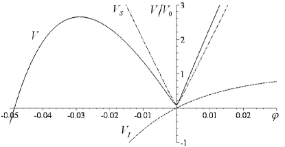
Figure 1: The inter-brane potential $V_{S}$ of (54), string gas potential $V_{I}$ of (55) and total potential $V=V_{I}+V_{S}$ with $d=6$, $n=4$. The height of $V$ at the minimum $\varphi=\sigma\approx 0$ is given by the momentum of the string gas along the three large dimensions $q$. We chose $l:=q/a=10^{-6}$ and $\tilde{N}/(V_{0}a^{3})=4\tilde{\alpha}/\beta$ for instructive reasons only, such that $V_{I}$, $V_{S}$ and $V$ are clearly discernable. Note that $V_{S}$ is only viable around $\varphi=\sigma$. In order for a minimum to exist and moduli trapping to occur, conditions (58) and (62) need to be satisfied.

This redshifting leads to a problem if we insist that the present day radion be stabilized by $V_{S}$, which can be seen as follows: let us for simplicity set $q=0$ for the time being and ask whether the total potential

$$V=V_{I}+V_{S}\,,$$ (56)

which is plotted in Fig. 1, exhibits a minimum. Expanding $V$ around $\varphi=0$ yields

$$V\approx V_{0}\tilde{\alpha}\varphi+\frac{\tilde{N}}{a^{3}}\left|\beta\varphi\right|\,.$$ (57)

In order to stabilize the radion at $\varphi=0$ we need

$$\frac{\tilde{N}}{a^{3}V_{0}}\gg\frac{\tilde{\alpha}}{\beta}=\mathcal{O}(1)\,,$$ (58)

so that the stabilizing potential $V_{S}$ is able to prevent the collapse of the internal dimensions due to the inter brane potential $V_{I}$. Since the universe expanded roughly another $60$ e-foldings after inflation until today, we would need

$$\frac{\tilde{N}}{V_{0}}\gg e^{180}$$ (59)

if we want a stable radion at late times, which is clearly an unreasonable condition. This problem is a simple reflection of the fact that the inter brane potential does not redshift, whereas the string gas redshifts like matter. Henceforth, it is not surprising that the attractive force between the branes wins in the long run. Notice that the same reason makes this type of stabilization incompatible with the presence of a cosmological constant Ferrer:2005hr .

If one insists on achieving stabilization via a string gas, there must be a mechanism present that cancels out $V_{I}$; luckily, such a mechanism seems possible in our scenario: once the branes associated with the orbifold fixed planes approach each other within the string scale they could annihilate via tachyon decay Sen:2002nu ; Sen:2002in ; Mukhopadhyay:2002en ; Rey:2003xs ; Chen:2002fp ; LLM ; Gutperle:2004be . It should be noted that the universe itself does not go through a singularity: the radion gets stabilized at the self dual radius so that there is no big crunch.

What is more, one can imagine that this decay contributes to pre-heating, similar to the mechanism employed in the cyclic/ekpyrotic scenario or in more recent realizations of brane inflation as in the KKLMMT proposal Kachru:2003sx ; Kofman:2005yz ; Chen:2006ni . However, this mechanism comes with a price: the potential over-production of relics like cosmic strings. If too many of these un-observed relics are produced, the model at hand would be ruled out Communication_SW_HF . Hence, we shall assume that a mechanism to cancel the inter brane potential exists without producing too many relics.

Since the redshifting of the string gas potential can potentially spoil stabilization at late times, it is a concern whether this redshifting will also spoil standard pre-heating methods or leave them unaffected. Thus, we will address this question in the next subsection.

IV.2 Pre-heating

Assuming that the inter brane potential cancels via some unspecified mechanism near the self dual radius, the complete potential for the radion is provided by the string gas alone, that is

$$V=\frac{N}{a^{3}}e^{-\frac{d}{2}\beta\varphi}\sqrt{\frac{q^{2}}{a^{2}}+\sinh^{2}(\beta\varphi)}\,.$$ (60)

We would now like to address the question whether the standard theory of pre-heating after inflation can be applied. The novel feature in our model is the dependence of the potential on the scale factor $a$. If one could neglect this feature, pre-heating would progress as usual, see e.g. Traschen:1990sw ; Shtanov:1994ce ; Kofman:1994rk ; Kofman:1997yn ; Greene:1997fu ; Felder:2000hj for a sample of the extensive literature on the subject.

As a first estimate we can compare the rate at which the potential changes with the Hubble factor. As we shall see below in (66), both quantities are of the same order. Hence we expect any effects due to the redshifting of the potential to be of the same magnitude as those directly caused by the expansion of the universe. As a consequence, whenever the Hubble expansion needs to be included, e.g. in the case of stochastic pre-heating Kofman:1997yn (broad parametric resonance in an expanding universe), one should also include the time dependence of the potential.

In order to examine more carefully whether the redshifting of an inflaton potential can be neglected under the assumption that the expansion of the universe itself is unimportant, we will focus on a specific toy model for pre-heating Kofman:1997yn ; Greene:1997fu : narrow parametric resonance Traschen:1990sw ; Shtanov:1994ce . It should be noted that narrow or broad parametric resonances will not be viable reheating mechanisms if the inflaton is identified with the radion (as in our case), since the couplings between the radion and other matter-fields are heavily suppressed . Nevertheless, we will focus on narrow resonance as an instructive example, since the mechanism is quite simple and very sensitive to changes in the shape of $V$: any change in the potential during the time-scale of pre-heating will cause the center of the resonance band to shift. If this shift is larger than the width of the resonance band, modes would not stay within the band long enough to get reasonably amplified. But if the shift is small compared to the width, narrow resonance will commence in the usual way. As we shall see below, the latter is the case so that there are no new effects and/or constraints due to the redshifting potential.

To study pre-heating, let us first expand the potential around the minimum of the potential at $\varphi_{min}=:\sigma$ and thereafter couple the radion to a scalar matter field $\chi$. At this first stage we neglect the expansion of the universe so that $n:=N/a^{3}\approx const$ and $l^{2}:=q^{2}/a^{2}\approx const$. The minimum of (60) can be found at

$$\sigma(l) = \frac{1}{2\beta}\ln\left(-3l^{2}+\frac{3}{2}-\frac{\sqrt{36(l^{4}-l^{2})+1}}{2}\right)\,,$$ (61)

Where we used $d=6$. Note that a minimum only exists for

$$0\leq l<\tilde{l}$$ (62)

with $\tilde{l}:=(\sqrt{12}-\sqrt{6})/6$, leading to $0\leq\sigma<\ln(2)/(4\beta)$. Expanding the potential around $\sigma$ leads to

$$V \approx \tilde{V}_{0}+\frac{m^{2}}{2}\phi^{2}\,,$$ (63)

where we used a shifted inflaton $\phi:=\varphi-\sigma$ and

$$\tilde{V}_{0}=ne^{-3\beta\sigma}\sqrt{l^{2}+\sinh^{2}(\beta\sigma)}\,,$$ (64)

as well as

$$m\approx\beta\sqrt{\frac{n}{l}}-\beta\frac{63}{4}\sqrt{n}l^{3/2}\,,$$ (65)

where we expanded $m$ around $l=0$. Note that $m(l=\tilde{l})\equiv 0$ exactly, so that any value of $m$ can be achieved by appropriately tuning $l$. We will not need the cumbersome exact expression for $m$ in the following, hence we shall omit it.

At this point we should step back for a second and estimate the rate of change of the potential. Using $l\propto 1/a$ and $q\propto 1/a^{3}$ we arrive at

$$\frac{\dot{m}}{m}\approx-H\,,$$ (66)

where we only kept the leading order term in (65). Hence, we naively expect that the expansion of the universe and the redshifting of the potential lead to comparable effects. This estimate can be made more concrete at the level of the toy model of narrow parametric resonance: if we couple the radion to a scalar matter field via $V_{int}=-g^{2}\phi^{2}\chi^{2}$, the system will be in the regime of narrow resonance if $g\Phi\ll\sigma\ll m$ holds, where $\Phi(t)$ is the amplitude of the oscillating inflaton Kofman:1997yn . This condition can be satisfied if we are free to tune $g$ and $m$ appropriately. Following the analysis of Kofman:1997yn closely, we find the first resonance band of the resulting Mathieu-equation for $\chi_{k}$ at the wave-number $k\approx m/2$ with a width of $\Delta k\approx\tilde{q}m/2$ where $\tilde{q}:=4g^{2}\sigma\Phi/m^{2}\ll 1$.

Since parametric resonance usually commences during the first few oscillations of $\phi$ around its minimum, the characteristic time-scale is given by the period of these oscillations $T=2\pi/m$.

Turning on the expansion of the universe yields the requirement

$$H\ll\tilde{q}^{2}m\,,$$ (67)

in order for narrow resonance to take place , otherwise modes would leave the resonance band too fast Kofman:1997yn . Given that inequality, we can give an upper bound on the change of the scale factor $a$ within the period $T$: because the scale factor makes a transition from an inflating one to a solution for a radiation dominated universe during pre-heating, we can use the inflationary solution as an upper bound for the change in $a$, that is

$$\frac{a(t_{0}+T)}{a(t_{0})}\approx e^{2\epsilon\pi\tilde{q}^{2}}$$ (68)

where we used $H\approx\epsilon\tilde{q}^{2}m$ with $\epsilon\ll 1$. This results in a change of the potential’s shape via a change in the inflaton mass

$$m(t_{0}+T) \approx \beta\sqrt{\frac{n}{l}}$$ (69)

$$\approx m(t_{0})e^{-\epsilon 2\pi\tilde{q}^{2}}$$ (70)

$$\approx m(t_{0})(1-\epsilon 2\pi\tilde{q}^{2})\,,$$ (71)

where we only kept the leading order term in $l$ from (65), plugged in $l\propto 1/a$ as well as $n\propto 1/a^{3}$ and expanded around $\tilde{q}=0$. Since the position of the first resonance band is located at $k=m/2$, we see that the shift of its position is given by $D_{k}=\epsilon\pi\tilde{q}^{2}m(t_{0})$. This shift has to be compared with the width of the band $\Delta k\approx\tilde{q}m(t_{0})/2$. We immediately see that $D_{k}\ll\Delta k$ and henceforth, we can safely ignore the slight change of the radion potential.

IV.3 Discussion

We saw in the previous section that the time dependence of the inflaton potential does not interfere much with the process of pre-heating. We estimated the effect on the toy model of narrow parametric resonance, because this pre-heating mechanism is most sensitive to changes in the mass of the inflaton. We found that new effects due to the redshifting potential are comparable to the ones already present due to the expanding universe.

Hence, we expect no novel features during pre-heating if a string gas supplies the stabilizing potential for the inflaton, and the standard theory of pre-heating can be applied (we refer the reader to Traschen:1990sw ; Shtanov:1994ce ; Kofman:1994rk ; Kofman:1997yn ; Greene:1997fu and follow up papers for the relevant literature). However, whenever the expansion of the universe itself is crucial, one should also consider the redshifting of the potential; for example, in the case of stochastic resonance Kofman:1997yn the Hubble expansion causes a mode to scan many resonance bands during a single oscillation of the inflaton. Naturally, including the redshifting of the potential will add to this effect, since the resonance bands themselves shift, just as in the case of narrow resonance we examined in the previous section.

There is another issue worth stressing again: since the inflaton is identified with the radion in our setup, its couplings to matter fields are heavily suppressed. As a consequence, we do not expect parametric resonance to be the leading pre-heating channel (see however Allahverdi:2004ge for the possibility of enhanced pre-heating), but instead tachyonic pre-heating (see e.g. Greene:1997ge ; Felder:2000hj ; Dufaux:2006ee and references therein), which occurs in case of a negative effective mass term for the matter field. This effect was used to address the moduli problem in Shuhmaher:2005mf and warrants further study Shu_prep .

Yet another possibility to reheat the universe could be provided by the annihilation of the boundary branes via tachyon decay Sen:2002nu ; Sen:2002in ; Mukhopadhyay:2002en ; Rey:2003xs ; Chen:2002fp ; LLM ; Gutperle:2004be once the branes come close to each other. A potential hinderance could be an over-production of relics such as cosmic strings. It seems possible to avoid this problem in certain circumstances Dasgupta:2004dw ; Chen:2005ae , but we postpone a study of this interesting possibility to a future publication, since it is beyond the scope of this article.

Last but not least, since the production of the stabilizing string gas will overlap with the early stages of pre-heating, one should discuss both processes in a unified treatment.

V Conclusions

In this article, we examined observational consequences of the recently proposed emerging brane inflation model. After reviewing the aforementioned model, observational parameters were computed within the slow roll regime, once and foremost the scalar spectral index $n_{s}=0.9659^{+0.0049}_{-0.0052}$. This index is a generic prediction of emerging brane inflation, independent of model specific details and in excellent agreement with recent constraints of WMAP3 and SDSS. Furthermore, based one the COBE normalization we were able derive a bound onto the fundamental string scale, (52).

Thereafter, we examined the consequences of a redshifting string gas potential, which arises at the end of inflation. Even though the radion/inflaton can initially be stabilized, the mechanism fails at late times as long as there is a contribution to the effective potential that does not redshift, like a cosmological constant or a remaining interbrane potential. Consequently, a mechanism to cancel out all such contributions needs to be found in order for the model to work.

Related to this mechanism, we encountered another potential problem: since the interaction of boundary branes is responsible for inflation, but branes have to be absent at late times in order to keep extra dimensions stable, we concluded that they had to annihilate after inflation. During this annihilation, which could in principle be responsible for pre-heating, relics like cosmic strings are expected to be produced. Mechanisms to avoid an overproduction of said relicts are conceivable, but warrant further study.

Concerned that pre-heating after inflation might also get disrupted via the time dependence of the potential, we focused on narrow parametric resonance as a toy model for pre-heating to estimate the magnitude of new effects: we find that new effects are comparable to those originating directly from the expansion of the universe. Henceforth, we concluded that the standard machinery of pre-heating can be applied to the model at hand, but the time dependence of the potential needs to be incorporated if expansion effects are crucial for pre-heating, as is the case in e.g. stochastic resonance. Since the annihilation of boundary branes and the production of the stabilizing string gas occurs during the early stages of pre-heating, one should incorporate these effects in a detailed study of pre-heating.

To summarize, the proposal of emerging brane inflation is a viable realization of inflation, if the potential problems associated with the annihilation of branes after inflation can be overcome.