Thermodynamics at the BPS bound for Black Holes in AdS

Abstract:

In this work we define a new limiting procedure that extends the usual thermodynamics treatment of Black Hole physics, to the supersymmetric regime. This procedure is inspired on equivalent statistical mechanics derivations in the dual CFT theory, where the BPS partition function at zero temperature is obtained by a double scaling limit of temperature and the relevant chemical potentials. In supergravity, the resulting partition function depends on emergent generalized chemical potentials conjugated to the different conserved charges of the BPS solitons. With this new approach, studies on stability and phase transitions of supersymmetric solutions are presented. We find stable and unstable regimes with first order phase transitions, as suggested by previous studies on free supersymmetric Yang Mills theory

1 Introduction

Classical Gravity shows many properties that are in fact thermodynamical in its very nature like for example Black Hole physics. In fact, General relativity (GR) can be thought as a thermodynamic theory of space-time, emerging at low energy regimes from a fundamental theory of space-time like string theory. This framework suggests that GR could be understood as a mean-field theory of thermodynamic nature.

Following this line of thoughts, it seems natural to approach quantum gravity, studding the statistical behaviour of the relevant ultraviolet degrees of freedom that in the infrared condense to GR (i.e. the search for a rational foundation of GR).

The search for such ultra-violet partons is a complicated task, and there is no clear answer of how to proceed. On the other hand, there is little doubt that string theory contains a quantum theory gravity, and delivers GR as an effective theory. The recurring unsolved problem is our incapacity to solve string theory, and hence understand the quantum gravity sector.

Within string theory, there are particularly simple systems where dramatic simplifications occur due to the existence of symmetries that effectively freezes almost all the degrees of freedom and dynamics. In these cases, some understanding has been archived resulting in the famous counting of microstates for a class of supersymmetric Black Holes, or even some extreme but not supersymmetric Black Holes [1, 2, 3].

The AdS/CFT duality [4, 5] also has contribute to improve our otherwise poor understanding of quantum gravity in the case where there is a negative cosmological constant. Here, there is a fully well defined quantum field theory ($SU(N)$ ${\cal N}=4$ SYM) that is equivalent to string theory with fixed asymptotic conditions in a negative cosmological constant background. It turns out that in the large $N$ limit, at strong ’t Hooft coupling, this field theory describes the GR sector.

In the literature there are many studies of quantum gravity and its dual significance in the CFT theory. Again, up to now ${\cal N}=4$ SYM theory at strong ’t Hooft coupling is too complicated to be fully comprehend and the program is far from completion. Nevertheless, the statistical approach to GR has concrete realization in studies on Black Holes in AdS, dual to finite temperature versions of the CFT, or in studies in particularly simple sectors of the CFT where due to symmetries progress is archived. For example see [6, 7, 8].

Recently, there were found supersymmetric Black Hole solutions in $AdS_{5}$ preserving only two real supercharges [9, 10, 11, 12, 13, 14]. These Black Holes (BH) provide a new arena were to search for microscopic signals of quantum gravity in the AdS/CFT framework. It would be very interesting to derive the entropy of such BH and in general understand its thermodynamical properties from the CFT point of view.

In [15], it was defined an index to count states in the CFT and also studied the statistical properties of the different supersymmetric sectors in the free theory limit. Unfortunately, the supersymmetric BH sector seems to be invisible to this new index, while the statistical analysis suggested that within the different BPS sectors there are complicated structures with instabilities and phase transitions some of which are related to Bose-Einstein condensations.

The aim of this work is to develop a framework where to study the statistical properties of supersymmetric solitons in AdS. To do this, we review some basic features of statistical mechanics with particular focus on the $T=0$ limit where supersymmetry appears. Then, as an example of the power of this new approach, we apply these techniques to study supersymmetric BH solutions in AdS. In the supersymmetric regime, we find a rich structure with phase transitions in a well defined ensemble picture that matches the canonical statistics analysis of dual CFT.

In section 2, we define the theoretical framework and the particular procedure to obtain the thermodynamics at the BPS bound. In section 3, we apply this procedure to the rotating BTZ BH [16] and the supersymmetric $AdS_{5}$ BH solutions found in [13], as main examples of the power of our new framework. In section 4, we begin the study on the stability and phase transitions of the above supersymmetric BH. A more profound study of the thermodynamic of the above BH with the corresponding comparison with the CFT partition function is currently under study[17]. At last, in section 5 we close with an overview, and a discussion on other BH solutions suggesting possible future directions

2 Statistical mechanics and thermodynamics in GR

Usually, the starting point of studies in statistical mechanics is the definition of the micro canonical ensemble. Here, all the physical states are label by a set of extensive quantities such as energy $E$, angular momentum $J$, electric charge $Q$, etc. Then it is assume that all states have the same probability to be measure. The partition function $\Xi_{(E,J,Q)}$ is defined as the total number of states in the ensemble, while the entropy $S$ is defined as

$$S=\ln\Xi_{(E,J,Q)}\quad\hbox{such that}\quad dS=\beta dE+\gamma dJ+\delta dQ\,,$$

where $(\beta,\gamma,\delta)$ are the conjugate variables of $(E,J,Q)$ respectively. In particular, note that the entropy doesn’t have to be zero at zero temperature, but in general is a function of the other charges.

To study the properties of the system, sometimes it is useful to exchange a few of the extensive variables with its conjugates partners by means of Legendre transformations. Such transformations have the physical interpretation of changing the type of ensemble (provided these maps are well defined, all ensembles are equivalent). In general, we have a grand canonical ensemble when some of the charges are replaced by their conjugated variables (here denoted in general as ”potentials”). For example, the form of the partition function $\Xi_{(\beta,\gamma,Q)}$ is

$$\Xi_{(\beta,\gamma,Q)}=\sum_{\nu}e^{(-\beta E_{\nu}-\gamma J_{\nu})}\,,$$

where the sum is over all states $\nu$ of the ensemble with fixed charge $Q$. The rational foundation of thermodynamics relies on the identification of all the empirical thermodynamical definitions like the different functions and laws, in terms of statistical mechanics concepts. In particular, working in the generalized grand canonical ensemble where all the charges have been replaced by the potentials, the following identification is obtained

$$-\ln\Xi_{(\beta,\Omega,\Phi)}=\beta E-\beta\Omega J-\beta\Phi Q-S\,,$$

where $\gamma=-\beta\Omega$, $\delta=-\beta\Phi$ and $\beta$ is the inverse of temperature $T$.

Consider now the case, where our theory is equipped with supersymmetry and we are interested to study its statistical properties. First of all, note that supersymmetric states form a subspace in the original Hilbert space of our theory. Therefore, we have to constraint the initial partition function to this supersymmetric hypersurface in order to account for the relevant statistical properties. One of the key point we want to stress and utilize along this work is that:

The supersymmetric partition function can be defined as a combination of limits for the different potentials, but not as the sole naive limit $\beta\rightarrow\infty$.

To make this clear, just note that all supersymmetric states are annihilated by a given set of supercharges. Therefore these states saturate a BPS inequality that translates into a series of constraints between the different physical charges. For definiteness, let us consider a simple example, where the BPS bound corresponds to the constraint $E=J$. This type of BPS bound appears in two dimensional supersymmetric models, like for example the effective theory of $1/2$ BPS chiral primaries of $N=4$ SYM in $R\otimes S^{3}$(see [18, 19, 20]). Then, defining the left and right variables

$$E^{\pm}=\hbox{$1\over 2$}(E_{\nu}\pm J_{\nu})\,,\quad\beta_{\pm}=(\beta\pm\gamma)\,,$$

$\Xi_{(\beta,\gamma,Q)}$ can be rewritten as

$$\Xi_{(\beta,\gamma,Q)}=\sum_{\nu}e^{-(\beta_{+}E_{+}+\beta_{-}E_{-})}\,.$$

At this point, it is clear that taking the limit $\beta_{-}\rightarrow\infty$ while $\beta_{+}\rightarrow\xi$ constant, gives the correct supersymmetric partition function. The above limiting procedure takes $T$ to zero, but also scales $\Omega$ in such a way that the new supersymmetric conjugated variable $\xi$ is finite and arbitrary. Note that among all available states, only those that satisfy the BPS bound are not suppress in the sum, resulting in the supersymmetric partition function

$$\Xi_{(\xi,Q)}=\sum_{\nu}e^{-\xi J}\,,$$

where the sum is over all supersymmetric states $\nu$ with $E=J$ at fixed charge $Q$ . The above argument shows how to find the relations between statistical mechanics and thermodynamics for supersymmetric configuration as a multi-scaling limit.

On the other hand, BH physics inspired a body of definitions and equations that effectively defines a thermodynamic theory in terms of space-time variables [21]. The missing step in this ”thermodynamics of space-time” is its rational foundation in terms of quantum gravity. In more detail, it has been shown that a semi classical approximation of the ”quantum gravity partition function” results in the exponential of the Euclidean supergravity action $I$, evaluated on the corresponding solitonic solution. The Euclidean action holds unexpected properties that interrelates it with other space-time variables such as Hawking temperature, energy, entropy, angular momentum, etc that defines the thermodynamics of space-time. In fact, $I$ plays the role of free energy divided by temperature and hence satisfies the equation

$$I=\beta E-\beta\Omega J-\beta\Phi Q-S\,,$$ (2.1)

sometimes called the ”quantum statistical relation” (QSR), where all quantities are evaluated on the particular solitonic solution of interest.

We point out that this thermodynamics is not only applicable to BH solutions, but seems to carry on to other solitonic solutions. Therefore we conjecture and use as a working hypothesis that:

the BH thermodynamics of space-time extends naturally to a general principle of space-time physics.

In fact, in [22] the very local GR equations where derived as equation of state of a generalization of BH thermodynamics that involves causal horizons. It is known, that the first law of BH thermodynamics is satisfied by a series of topological solitons that do not look like a BH [23]. To be more precise, we are thinking to include all solitons with any temperature, even zero (like extreme and supersymmetric solutions BH), topological solitons (where there is no horizon at all!), etc.

In this work we will apply the above conjecture to supersymmetric BH solutions in AdS and its non-supersymmetric extensions [13]. The reason behind this pragmatic approach is to open up a new mechanism to investigate on $1/2,1/4,1/8$ and $1/16$ supersymmetric configurations in the AdS/CFT duality and try to find traces of a microscopic description of the QSR.

Since we want to study supersymmetric solitons, the first task we face is how to recover the $T=0$ thermodynamics in the GR framework. Note that in the supersymmetric limit, the thermodynamic potentials are independent of physical observables (like charge, energy, etc). For example, in a BPS rotating BH, the angular velocity of the horizon $\Omega$, equals the velocity of light regardless its mass or angular momentum[24]. The same happens to the electrostatic potential $\Phi$ that also can be understood as angular velocity once the solution is uplift to ten or eleven dimensions. Therefore, for BPS solutions, we do have some thermodynamical variables at our disposal, like entropy and conserved charges, but we seem to lack of thermodynamical potentials.

Nevertheless, in our previous discussions of supersymmetric limits in statistical mechanics, we learned that the correct procedure is to consider a combined limit of the different off-BPS potentials. Accordingly, taking the QSR equation it is easy to see that if the charges behave as

$$E\rightarrow E_{bps}+O(\beta^{-2})\,,\quad J\rightarrow J_{bps}+O(\beta^{-2})\,,\quad Q\rightarrow Q_{bps}+O(\beta^{-2})\,$$ (2.2)

things will not work correctly unless the GR potentials behave as

$$\beta\rightarrow\infty\,,\quad\Omega\rightarrow\Omega_{bps}-{w\over\beta}+O(\beta^{-2})\,,\quad\Phi\rightarrow\Phi_{bps}-{\phi\over\beta}+O(\beta^{-2})\,,$$ (2.3)

where the ”$bps$” subscript defines the corresponding supersymmetric values. If the above general behaviour is not archived by the soliton under study, the supersymmetric limit will no be recover, showing a breakdown of our conjecture on the general nature of the thermodynamical properties of space-time or a failure of the GR description of the corresponding soliton.

Assuming that the above relations hold, we get the following expression

$$I=\beta\left(E_{bps}-\Omega_{bps}J_{bps}-\Phi_{bps}Q_{bps}\right)+wJ_{bps}+\phi Q_{bps}-S_{bps}+O(\beta^{-1})\,.$$

since the first term multiplying $\beta$ is identically zero due to the BPS property of the limiting solution, we end up with the ”supersymmetric version of the the quantum statistical relation” (SQSR)

$$I_{bps}=wJ_{bps}+\phi Q_{bps}-S_{bps}\,,$$

The above definitions of supersymmetric potentials and the SQSR are a concrete realization of our new perspective in the BH thermodynamics. Armed with these new objects, we can study the different thermodynamical properties of BPS solitons and compare them with the dual statistical behaviour.

In the following section, we will check that the above framework is verified and that indeed the BPS potentials and the SQSR are well defined for AdS solitons. Then, we start the study of its thermodynamical consequences, like stability and phase transitions.

3 Thermodynamics of supersymmetric solitons in AdS

The aim of this section is to test the general properties derived before. In the long run, we are interested in supersymmetric solutions of five dimensional gauge supergravity because these solutions can be also studied via its holographic relation to N=4 SYM theory extending studies like [15]. Supersymmetric BH solutions in $AdS_{5}$ were found first in [10, 11] and then in [12, 13, 14]. Recently, in [9] all the families were generalized to a single solution. Unfortunately, only the solutions of [12] and those of [14] are known in an off-BPS regime. There are other $AdS_{5}$ BH solution like [25, 26, 27] that have ill defined BPS limits. In these later cases, the BPS limit degenerate to naked singular solutions that are believe to get stringy corrections, that in turn should cure this behaviour either dressing the singularity with an event horizon or smoothing it out. Also, in a different framework, we have the BTZ BH solution [16], that has a well defined supersymmetric limit and has been extensively studied in the $AdS_{3}/CFT_{2}$ correspondence.

Our strategy is plain and simple. Given a solution that contains a well defined BPS regime, we find an adequate description of its off-BPS character. Then, we expand around it to recover the SQSR and the corresponding supersymmetric potentials. At this point, we should be ready to investigate its statistical dynamical properties like phase transitions and instabilities.

In this work, we will deal with BH solutions that have well behaved supersymmetric limits, like the BTZ BH and the solutions of [13].

3.1 Statistical properties of rotating BTZ Black Hole at T=0

As a first example, we start our studies with the rotating BTZ BH solution [16]. This BH appears naturally as the near horizon geometry of a system of $Q_{1}$ D1-branes, $Q_{5}$ D5-branes and a wave with momentum $N$. Therefore lies within the $AdS_{3}/CFT_{2}$ correspondence. The rotating BTZ metric can be written as

$$ds^{2}=-{(r^{2}-r_{+}^{2})(r^{2}-r_{-}^{2})\over r^{2}}\,dt^{2}+{r^{2}l^{2}\over(r^{2}-r_{+}^{2})(r^{2}-r_{-}^{2})}\,dr^{2}+r^{2}(d\phi+{r_{+}r_{-}\over r^{2}}\,dt)\,.$$

The energy $E$ and angular momentum $J$ are given by

$$E={k\over 2l^{2}}(r_{+}^{2}+r_{-}^{2})\quad\hbox{and}\quad J={k\over l^{2}}(r_{+}r_{-})\,,$$

where $k=Q_{1}Q_{5}$ is used since equals the level of the dual Kac-Moody superconformal algebra and $l$, the radius of $AdS_{3}$ is also a function of $Q_{1}\,,Q_{5}$, the string coupling constant and the compactified four dimensional volume. The above BH has an internal horizon at $r_{-}$ and external horizon at $r_{+}$. The supersymmetric limit is recovered when the energy equals the angular momentum, resulting in the collapse of both horizons i.e. $r_{+}=r_{-}$.

In [28], a very convenient description is given in terms of the left and right temperatures $(T_{+},T_{-})$ of the dual CFT theory, such that $r_{\pm}=\pi l(T_{+}\pm T_{-})$. Then all the relevant thermodynamic potentials like the Hawing temperature $T$, angular velocity of the external horizon $\Omega$, entropy $S$ and charges $E$ and $J$, can be written in terms of $T_{+}$ and $T_{-}$ as follows

$$\beta\equiv{1\over T}=({1\over 2T_{+}}+{1\over 2T_{-}})\,,\quad\Omega=\left({T_{+}-T_{-}\over T_{+}+T_{-}}\right)\,,\quad E={\pi^{2}k\over 2l^{2}}(T_{+}^{2}+T_{-}^{2})\,,$$

$$J={\pi^{2}k\over 2l^{2}}(T_{+}^{2}-T_{-}^{2})\,,\quad S=2\pi^{2}k(T_{+}+T_{-})\,.$$

We are interested in the $T_{-}=0$ limit of the above soliton and in particular in the corresponding QSR equation 2.1. The expansion in terms of the off-BPS parameter $T_{-}$ of the relevant thermodynamic variables gives

$$\beta\rightarrow{1\over 2T_{-}}+{1\over 2T_{+}}\,,\quad\Omega\rightarrow 1-{2\over T_{+}}T_{-}+O(T_{-}^{2})\,,\quad S\rightarrow 2\pi^{2}kT_{+}+O(T_{-}^{1})\,,$$

$$E\rightarrow\pi^{2}kT_{+}^{2}+O(T_{-}^{2})\,,\quad J\rightarrow\pi^{2}kT_{+}^{2}+O(T_{-}^{2})\,.$$

The above expansion defines the BPS value for the $E$, $J$ and $S$ as $E_{bps}=J_{bps}=\pi^{2}kT_{+}^{2}$ and $S_{bps}=2\pi^{2}kT_{+}$. Also as explain in the previous section, the BPS value of $\Omega$ is independent of the supersymmetric BH parameter $T_{+}$ and evaluates to 1. Collecting term together for the QSR we get that

$$I=\left({1\over 2T_{-}}\right)\left(E_{bps}-J_{bps}\right)+\left({1\over 2T_{+}}\right)\left(E_{bps}-J_{bps}\right)+\left({1\over T_{+}}\right)J_{bps}-S_{bps}+O(T_{-}^{1})\,,$$

from with we deduce that the finite part $I_{bps}$, corresponding to the BPS action satisfies the SQSR equation

$$I_{bps} =wJ_{bps}-S_{bps}\,,$$

$$=-\pi^{2}kT_{+}\,,$$

where $w=1/T_{+}$. Note that the action $I_{bps}$ is a negative function for all $T_{+}>0$ showing stability and no phase transitions with a very simple behaviour.

Nevertheless, this first example shows that in fact the theoretical framework considered in the previous section, has an explicit realization in the rotating BTZ BH. In principle, there is no a priory reason why the supergravity solution has to follow an expansion like (2.2) and (2.3). This is a non trivial test on our conjecture for the general nature of the thermodynamics of space-time.

Also, in this particular case it is remarkable that the thermodynamic potential $w$ matches exactly the inverse of the CFT dual left temperature $T_{+}$, in a striking parallelism to the CFT statistical description of this supersymmetric sector (again, see [28] for the dual CFT description).

3.2 Statistical properties of $AdS_{5}$ Black Holes at T=0

Let us consider next, solitons on $AdS_{5}$ that are dual to $SU(N)$ $\mathcal{N}=4$ SYM in four dimensions. The solution we consider here was first presented in [12]. In the BPS regimen, these solutions preserved only a fraction of $1/16$ of the total $32$ supercharges, and depending on the different range of values of its parameter space, describe BPS BH or topological solutions with no horizon.

In general, the solution comes with two independent angular momenta $(J_{1},J_{2})$, and a single electric charge $Q$ . In terms of Boyer-Lindquist type coordinates $x^{\mu}=(t,r,\theta,\phi,\psi)$ that are asymptotically static (i.e. the coordinate frame is non-rotating at infinity), the metric and gauge potential are

$$ds^{2} = -{\Delta_{\theta}\,[(1+g^{2}r^{2})\rho^{2}dt+2q\nu]\,dt\over\Xi_{a}\,\Xi_{b}\,\rho^{2}}+{2q\,\nu\omega\over\rho^{2}}+{f\over\rho^{4}}\Big{(}{\Delta_{\theta}\,dt\over\Xi_{a}\Xi_{b}}-\omega\Big{)}^{2}+{\rho^{2}dr^{2}\over\Delta_{r}}+$$

$$\quad\,\quad+{\rho^{2}d\theta^{2}\over\Delta_{\theta}}+{r^{2}+a^{2}\over\Xi_{a}}\sin^{2}\theta d\phi^{2}+{r^{2}+b^{2}\over\Xi_{b}}\cos^{2}\theta d\psi^{2}\,,$$

$$A = {\sqrt{3}q\over\rho^{2}}\,\Big{(}{\Delta_{\theta}\,dt\over\Xi_{a}\,\Xi_{b}}-\omega\Big{)}\,,$$

where

$$\Delta_{r} = {(r^{2}+a^{2})(r^{2}+b^{2})(1+g^{2}r^{2})+q^{2}+2abq\over r^{2}}-2m\,,$$

$$\Delta_{\theta} = 1-a^{2}g^{2}\cos^{2}\theta-b^{2}g^{2}\sin^{2}\theta\,,\quad f=2m\rho^{2}-q^{2}+2abqg^{2}\rho^{2}\,,$$

$$\rho^{2} = r^{2}+a^{2}\cos^{2}\theta+b^{2}\sin^{2}\theta\,,\quad\Xi_{a}=1-a^{2}g^{2}\,,\quad\Xi_{b}=1-b^{2}g^{2}\,,$$

$$\nu = b\sin^{2}\theta d\phi+a\cos^{2}\theta d\psi\,,\quad\omega=a\sin^{2}\theta{d\phi\over\Xi_{a}}+b\cos^{2}\theta{d\psi\over\Xi_{b}}\,.$$

The relevant thermodynamical potentials are

$$\beta={2\pi r_{+}\,[(r_{+}^{2}+a^{2})(r_{+}^{2}+b^{2})+abq]\over r_{+}^{4}[(1+g^{2}(2r_{+}^{2}+a^{2}+b^{2})]-(ab+q)^{2}}\,,\quad\Phi={\sqrt{3}qr_{+}^{2}\over(r_{+}^{2}+a^{2})(r_{+}^{2}+b^{2}+abq)}\,,$$

$$\Omega_{1}={a(r_{+}^{2}+b^{2})(1+g^{2}r_{+}^{2})+bq\over(r_{+}^{2}+a^{2})(r_{+}^{2}+b^{2})+abq}\,,\quad\Omega_{2}={b(r_{+}^{2}+a^{2})(1+g^{2}r_{+}^{2})+aq\over(r_{+}^{2}+a^{2})(r_{+}^{2}+b^{2})+abq}\,.\quad\quad$$

while the conserved charges are

$$E={m\pi(2\Xi_{a}+2\Xi_{b}-\Xi_{a}\,\Xi_{b})+2\pi qabg^{2}(\Xi_{a}+\Xi_{b})\over 4\Xi_{a}^{2}\,\Xi_{b}^{2}}\,,\quad Q={\sqrt{3}\,\pi q\over 4\Xi_{a}\,\Xi_{b}}\,,$$

$$J_{a}={\pi[2am+qb(1+a^{2}g^{2})]\over 4\Xi_{a}^{2}\,\Xi_{b}}\,,\quad J_{b}={\pi[2bm+qa(1+b^{2}g^{2})]\over 4\Xi_{b}^{2}\,\Xi_{a}}\,.\quad$$

Finally the entropy is given by

$$S={\pi^{2}[(r_{+}^{2}+a^{2})(r_{+}^{2}+b^{2})+abq]\over 2\Xi_{a}\Xi_{b}r_{+}}\,.$$

In all the above expressions, $r_{+}$ is largest positive root of $\Delta_{r}=0$. Also for convenience, in the rest of the paper we will set the $AdS$ radius to 1 i.e. $g=1$.

The BPS limit is achieved if

$$E-J_{a}-J_{b}-\sqrt{3}\,Q=0$$

that in terms of the for parameters $(m,q,a,b)$ translates into $q(1+a+b)=m$.

As we said before, in the BPS limit, we not only have BH solutions, but topological solutions, naked singular solutions, and even over-charge and over-rotating solutions containing pathologies like closed time-like curves. To define the correct BPS limit we have to avoid the forbidden regions in the moduli space of the solutions. At the end, in the BPS regime there are two types of regular solitons, BH and topological solutions.

BPS BH solutions

We have found that the following procedure does take us safely to the BPS BH solutions. Define the off-BPS parameter $\mu$ such that $m=m_{bps}+\mu\quad\hbox{where}\quad m_{bps}=q((1+a+b)$. To avoid the over-charged regimes that produce pathological solutions with CTC, is enough to impose the constraint $q=(1+a)(1+b)(a+b)$. As a result of the above, we have reduced the number of independent parameters from the original four $(m,q,a,b)$ to three $(\mu,a,b)$ out of which $\mu$ controls the off-BPS nature of the solution. Summarizing we have

$$m=q(1+a+b)+\mu\,,\quad q=(1+a)(1+b)(a+b)\,.$$

With the above parametrization is straight forward to expand all the thermodynamic quantities in terms of $\mu$, obtaining for the potentials

$$\beta = \left({\pi q\sqrt{r_{bps}^{2}+(1+a+b)^{2}}\over\sqrt{2}(3r_{bps}^{2}+1+a^{2}+b^{2})}\right){1\over\sqrt{\mu}}+O(0)\,,$$

$$\Phi = \sqrt{3}+\left({\sqrt{6}(ab-1)\over(1+a)(1+b)\sqrt{[r_{bps}^{2}+(1+a+b)^{2}]r_{bps}^{2}}}\right)\sqrt{\mu}+O(1)\,,$$

$$\Omega_{1} = 1+\left({\sqrt{2}(a-1)(a+2ab+b^{2}+2b)\over q\sqrt{[r_{bps}^{2}+(1+a+b)^{2}]r_{bps}^{2}}}\right)\sqrt{\mu}+O(1)\,,$$

$$\Omega_{2} = 1+\left({\sqrt{2}(b-1)(b+2ab+a^{2}+2a)\over q\sqrt{[r_{bps}^{2}+(1+a+b)^{2}]r_{bps}^{2}}}\right)\sqrt{\mu}+O(1)\,,$$

and for the conserved charges and entropy

$$E=E_{bps}+O(1)\,,\quad J^{1}=J_{bps}^{1}+O(1)\,,\quad J^{2}=J_{bps}^{2}+O(1)\,,$$

$$Q=Q_{bps}\,,\quad S=S_{bps}+O(1)\,,\qquad\qquad\qquad$$

where

$$E_{bps} = {\pi(a+b)(1-a)(1-b)+(1+a)(1+b)(2-a-b)\over 4(1-a)^{2}(1-b)^{2}}\,,$$

$$J_{bps}^{1} = {\pi(a+b)(2a+b+ab)\over 4(1-a)^{2}(1-b)}\,,\quad J_{bps}^{2}={\pi(a+b)(a+2b+ab)\over 4(1-a)(1-b)^{2}}\,,$$

$$Q_{bps}={\sqrt{3}\pi(a+b)\over 4(1-a)(1-b)}\,,\quad S_{bps}={\pi^{2}(a+b)r_{0}\over 2(1-a)(1-b)}\,,$$

with $r_{bps}^{2}=a+b+ab$, corresponding to the position of the BPS horizon.

Evaluating the above expansion into the QSR, we get

$$I_{bps}=\phi Q_{bps}+w_{1}J_{bps}^{1}+w_{2}J_{bps}^{2}-S_{bps}$$

where

$$w_{1}={\pi(1-a)(a+2ab+b^{2}+2b)\over r_{bps}(3r_{bps}^{2}+1+a^{2}+b^{2})}\,,\quad w_{2}={\pi(1-b)(b+2ab+a^{2}+2a)\over r_{bps}(3r_{bps}^{2}+1+a^{2}+b^{2})}\,,$$

$$\phi={\pi\sqrt{3}(a+b)(1-ab)\over r_{bps}(3r_{bps}^{2}+1+a^{2}+b^{2})}\,.\qquad\qquad\qquad\qquad$$

Let us consider what we have archived up to now. In first place, the expansion in the off-BPS parameter $\mu$ has reproduce the exact behaviour, anticipated in the general discussion, that defines the SQSR for supersymmetric solitons. This is not a trivial fact, since there is no reason a priory why things should work as they do. It is simply another surprise of GR and another confirmation of its thermodynamical nature. Second, in doing the expansion, we have obtained the definition of the corresponding supersymmetric potentials $(\phi,w_{1},w_{2})$. Naturally these potentials comes as functions of the parameters $(a,b)$, mimicking exactly the usual statistical dynamics derivation in the CFT. These potentials are the variables that in the thermodynamical sense, define the Generalized Grand canonical ensemble at zero temperature. Third, with this new framework, we are able to study the stability and phase transitions of the above solutions.

BPS topological solutions

For the topological soliton sector, we have found that the following procedure does take us safely to the BPS regime. As before, define the off-BPS parameter $\mu$ such that $m=m_{bps}+\mu\quad\hbox{where}\quad m_{bps}=q((1+a+b)$ but now, to avoid the over-charged regimes that produce pathological solutions with CTC, is enough to impose the constraint $q=-(1+a)(1+b)(a+2b+ab)(b+2a+ab)$. This choice of constraints, should be accompanied with the coordinate transformation $R=r^{2}-r_{bps}^{2}$, where $\Delta_{r}(r_{bps})=0$, since $r_{bps}^{2}=-(a+b+ab)^{2}$. As a result of the above, we have reduced the number of independent parameters from the original four $(m,q,a,b)$ to three $(\mu,a,b)$ out of which $\mu$ controls the off-BPS nature of the solution. Summarizing we have

$$m=q(1+a+b)+\mu\,,\quad q=-(1+a)(1+b)(a+2b+ab)(b+2a+ab)\,.$$

Next, we expand all the thermodynamic quantities in terms of $\mu$, obtaining for the potentials

$$\beta = \left({2\pi(2r_{bps}^{2}+a^{2}+b^{2})\over r_{bps}^{3}(1+a+b+2r_{bps}^{2})}\right)\mu+O(2)\,,$$

$$\Phi = \left({\sqrt{3}qr_{bps}^{2}\over(1+a+b+2r_{bps}^{2})}\right){1\over\mu}+{\sqrt{3}q\over(1+a+b+2r_{bps}^{2})}+O(1)\,,$$

$$\Omega_{1} = \left({a(r_{bps}^{2}+b^{2})(1+r_{bps}^{2})\over(1+a+b+2r_{bps}^{2})}\right){1\over\mu}+{a(2r_{bps}^{2}+1+b^{2})\over(1+a+b+2r_{bps}^{2})}+O(1)\,,$$

$$\Omega_{1} = \left({b(r_{bps}^{2}+a^{2})(1+r_{bps}^{2})\over(1+a+b+2r_{bps}^{2})}\right){1\over\mu}+{b(2r_{bps}^{2}+1+a^{2})\over(1+a+b+2r_{bps}^{2})}+O(1)\,,$$

for the conserved charges

$$E=E_{bps}+O(1)\,,\quad J^{1}=J_{bps}^{1}+O(1)\,,\quad J^{2}=J_{bps}^{2}+O(1)\,,\quad Q=Q_{bps}\,,$$

where

$$J_{bps}^{1}=-{\pi(2b+a+ab)(2a+b+ab)^{2}\over 4(1-a)^{2}(1-b)}\,,\quad J_{bps}^{2}=-{\pi(2b+a+ab)^{2}(2a+b+ab)\over 4(1-a)(1-b)^{2}}\,,$$

$$Q_{bps}=-{\sqrt{3}\pi(2b+a+ab)(2a+b+ab)\over(1-a)(1-b)}\,,\quad E_{bps}=\sqrt{3}Q_{bps}+J_{bps}^{1}+J_{bps}^{2}$$

and finally the entropy S gives

$$S=\left({\pi(2r_{bps}^{2}+a^{2}+b^{2})\over 2r_{bps}(1-a^{2})(1-b^{2})}\right)\mu+O(2)\,.$$

Note the strange responds of all the thermodynamic functions to the off-BPS expansion. $\beta$ goes to zero while all the potential diverge, but in such a way the the physical quantity $\beta\Omega$ or $\beta\Phi$ has a finite value. Although this behaviour seems counterintuitive, we point out that these specific combinations of $\beta\Omega$ and the others, are the physical periods of the angular variables in the Euclidian regime (see section three in [24]), and therefore is reasonable kept them constant along the expansion.

Evaluating the above off-BPS expansion into the QSR, we get

$$I_{bps}=\phi Q_{bps}+w_{1}J_{bps}^{1}+w_{2}J_{bps}^{2}\,,$$

where

$$w_{1}=-{2\pi a(r_{bps}^{2}+b^{2})(r_{bps}^{2}+1)\over r_{bps}^{3}(1+a^{2}+b^{2}+2r_{bps}^{2})}\,,\quad w_{2}=-{2\pi b(r_{bps}^{2}+a^{2})(r_{bps}^{2}+1)\over r_{bps}^{3}(1+a^{2}+b^{2}+2r_{bps}^{2})}\,,$$

$$\phi=-{2\sqrt{3}\pi q\over r_{bps}^{3}(1+a^{2}+b^{2}+2r_{bps}^{2})}\,.\qquad\qquad\qquad\qquad$$

Unfortunately this is not the end of the story, since in the above solution; we still have to impose another constraint to avoid a conical singularity,

$$3(1+b)(2+b)a^{2}+2(4b^{2}+7b+1)a+(5b+1)=0\,.$$

This equation can be easily solved for $b$, to give $a=-b/(2+b)$ or $a=-(5b+1)/(3+3b$. The firs option gives pure AdS space, so we concentrate in the second option. The evaluation of the different charges and potential is not difficult but tedious, here we the final results first for the charges,

$$J_{bps}^{1}={(b^{2}+4b+1)^{2}\over 48(2b+1)^{2}}\,,\quad J_{bps}^{2}={(b^{2}+4b+1)\over 72(2b+1)}\,,\quad Q_{bps}=-{\sqrt{3}(b^{2}+4b+1)\over 24(2b+1)}\,,$$

$$E_{bps}=\sqrt{3}Q_{bps}+J_{bps}^{1}+J_{bps}^{2}\,,\qquad\qquad\qquad\qquad\qquad$$

and for the potentials,

$$w_{1} = {8(5b+1)(1+b)(5b^{2}-4b-1)(b^{2}+b-2)\over(b^{4}-6b^{3}+17b^{2}+16b+8)(2b+1)^{3}}\,,$$

$$w_{2} = {96b^{2}(b^{2}+b-2)(b^{3}+3b^{2}-3b-1)\over(b^{4}-6b^{3}+17b^{2}+16b+8)(2b+1)^{3}}\,,$$

$$\phi = {8\sqrt{3}\pi(1-b)^{2}(1+4b+b^{2})\over(1+b)(2b+1)^{3}}\,.$$

Again, as in the previous case we have found a finite expression for the SQRS in terms of the supersymmetric charges and the conjugated potentials. Note that as expected, in this case there is no entropy. This solutions are in this sense like the regular LLM solutions of the $1/2$ BPS sector [29], where there is a well defined ensemble of chiral primaries exited, that do not produce a sizeable entropy for regular solutions (see [30] for more comments).

4 Stability and Phase transitions

The definition of the SQSR permits the study of the semi classical partition function, as we vary the different chemical potentials depending on the case of study. Like in the dual conformal field theory at T=0, we have a rich physical structure with phase transitions where the BH soliton is not any more the dominant soliton, as in fact occurs in the dual CFT for $1/16$ supersymmetric sectors.

Before presenting the stability analysis, it is important to realized that these solitons are not the most general $1/16$ supersymmetric solutions. In the dual CFT, general states in the $1/16$ supersymmetric representation depend of three R-charges and two angular momenta. Even if we look for states with the same R-charges, there is no need of an extra constraint relating the two angular momenta and the electric charge. On the other hand, for five dimensional gauge supergravity with 32 real supercharges, we should have three different electric charges plus two angular momenta, giving a grand total of five independent degrees of freedom. In the supergravity soliton, all the electric charges are collapsed into one and on the top of this, we have to impose a relation between the electric charge and two angular momenta, to avoid CTC or naked singularities. Therefore, it is reasonable to expect that there should be more general solutions waiting to be discovered.

Keeping the above fact in mind, we proceed to study this solution, that are the best we can do to scan the physical structure in the $1/16$ BPS sector from the supergravity point of view. Basically we are working in a constraint hypersurface of the full space of supersymmetric BH solutions.

4.1 BPS BH solutions

Evaluation of the $I_{bps}$ in this case gives

$$I_{bps}={\pi^{2}(a+b)^{2}[-1+2b+b^{2}+b^{2}+a(2+5b+b^{2})+a^{2}(1+b)]\over 4(1-a)(1-b)\sqrt{a+b+ab}(1+a^{2}+b^{2}+3(a+b+ab))}\,,$$

where the range of the parameters $(a,b)$ is obtained from the physical condition that $r_{bps}^{2}\geq 0$ or equivalently $a+b+ab\geq 0$,$(a,b)\leq 1$. The first inequality is the condition that the position of the horizon is well defined and the second comes from our normalization of the AdS radius.

In figure (fig. 1), we show a three dimensional plot of $I_{bps}$ as a function of $(a,b)$.

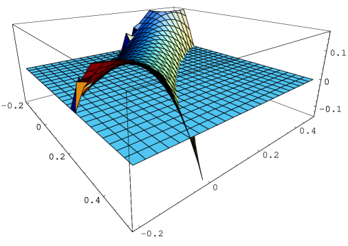
Figure 1: Plot of the Euclidean action of the BPS BH as a function of the parameters $(a,b)$. The flat plane corresponds zero level surface.

In the plot, it is easy to see that $I_{bps}$ is positive for small $(a,b)$ and negative for larger values. From which we deduce that there is a phase transition, where the BH solution is not any more the preferred vacuum, but a meta-stable vacuum. In (fig. 2) we show a two dimensional plot for $b=.1$ where the change of sign of $I_{bps}$ is more explicit. We are not sure what is the stable vacuum, perhaps is one of the more general solutions that still we do not know or perhaps is probably related to a gas of superparticlas in AdS, studied in detail in [15].

Figure 2: Plot of the Euclidean action at fixed $b=1/10$.

After the above global analysis, we consider the local stability criteria (see for example [31, 32, 33, 34, 35, 36]), base on the behavior of different susceptibilities that are generalization alike the more traditional specific heat in the canonical ensemble. There are many different ways introduce the local stability analysis, but it can always be related to the second law of thermodynamics where the entropy is a local maximum of a stable equilibrium configuration. For example, we consider the so-called ”isothermal permittivity” $\epsilon$,

$$\epsilon=-\left({\partial Q\over\partial\phi}\right)_{T=0}$$

that relates the change of electric charge to the change of its chemical potential $\phi$. In (fig. 3) we show a plot of $\epsilon$ as a function of $(a,b)$, where it can be seen a first order transition characterizing the phase transition. Also for more clarity we show a two dimensional plot of $\epsilon$ at $b=.1$ as a function of $a$, where the system is symmetric with respect to $(a,b)$.

Other susceptibilities can be introduced, but we believe that the above calculation illustrates well enough the thermodynamical properties of the solution in the grand canonical ensemble.

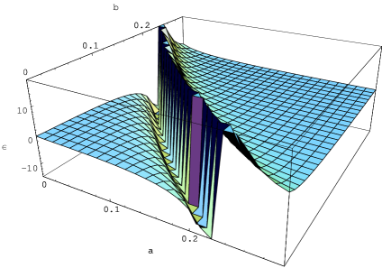
Figure 3: Plot of the susceptibility $\epsilon$ for $b=1/10$.

Figure 4: Plot of the susceptibility $\epsilon$ for $b=1/10$.

4.2 BPS solitonic solutions

In this case, Evaluation of the $I_{bps}$ gives

$$I_{bps}={(b-1)^{2}(b^{2}+4b+1)^{2}(29b^{5}+232b^{4}+54b^{3}-174b^{2}-167b-46)\over 6(b+1)(2b+1)^{5}(b^{4}-6b^{3}+17b^{2}+16b+8)}\,,$$

where after some inspection, it is not difficult to see that among all the possible ranges of $b$, the interval $\left((10-\sqrt{139})/3,-1/2\right)$ covers all the physical possibilities. The other values of $b$, correspond either to repetitions of the relevant physical situation or produce solutions with negative energy that we ruled out.

In figure (fig. 5) and (fig. 6), we show a plot of $I_{bps}$ as a function of $(b)$ for this topological case. In the plots, it can be seen that the $I_{bps}$ is positive in the first plot while negative in the second. Therefore we again have a situation where the solitonic solutions is unstable, and another where it is stable.

We have found that at the point $b=-1/2$ the plot really shows a break down of our expansion on the off-BPS parameter $\mu$. Basically, at $b=-1/2$ we have done a ”division by zero” and our expression for $I_{bps}$ is not to be trust. Nevertheless, the problem appears only at this very point, and we have checked that it is possible to redefine a specific off-BPS expansion around this particular point. Here we have not included such a detail analysis since, in any case, the change of sign is warranty because the expansion work fine away of $b=-1/2$.

The technical complications with the off-BPS expansion at the point $b=-1/2$ prevent us to consider a local analysis of the phase transition. This sort of studies will be covered in a following work, where more extensive studies on the thermodynamic properties of this and another family of solutions will be reported [17].

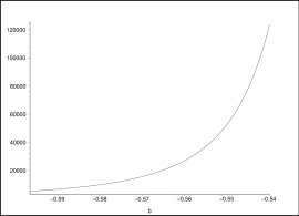
Figure 5: This plot cover the first half of the allowed range for $b$.

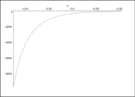
Figure 6: This plot cover the second half for the allowed range of $b$

5 Discussion

In this work, we have defined a framework to study thermodynamics properties in the BPS regime for general supersymmetric solitons in gauge supergravity. The mechanism is suggested by the equivalent more standard studies in supersymmetric field theories. In particular due to the AdS/CFT duality, this kind of reasoning acquires firmer grounds that support it.

To perform this analysis, we fund natural to assume that the thermodynamic properties of the solitonic solutions in supergravity are a fundamental characteristic that does not apply only to solutions with non zero surface gravity and horizons like the standard BH, but extends to supersymmetric solitons, with or with out horizons at zero temperature. In other words,

the BH thermodynamics of space-time extends naturally to a general principle of space-time physics.

In practice, how to extend the BH thermodynamics definitions is not that clear. Here we found that things analogous to chemical potentials to the different conserved charges do have an extension. Again, the AdS/CFT duality also supports this generalization since statistical mechanics is well defined in the dual CFT theory and therefore should have a counterpart in the supergravity side.

In fact, we have found explicit realizations of this mechanism and framework in different types of supersymmetric solutions of different supergravity theories, like the rotating BTZ BH in three dimensions or the AdS BH in five dimensions. In all the examples here studied, the limiting procedure gives finite quantities that play the role of thermodynamical variables in the BPS regime.

In particular, we arrive to the definition of BPS chemical potentials that where unknown up to now in the literature. For the rotating BTZ BH, the BPS chemical potential corresponds exactly to the inverse of the left temperature in the dual two dimensional CFT, an encouraging signal that this BPS chemical potentials are physical quantities that deserve attention. For the other studied cases, we do not know their role in the CFT dual picture, so more work is needed to address this important question.

We have also fund a rich structure of phase transitions among our BPS examples. In particular the five dimensional soliton shows for the BH case, a clear first order phase transition to another soliton that is either a new solution that we do not know about or simply a gas of superparticles in AdS. For the topological solution, we found a instability, but where unable to determine its order due to technical details.

The present work is just the initial step to study the BPS phase space for BH in AdS. Here, we have defined the framework and minimal machinery to obtain the phase diagrams. Then with a couple of examples, we have checked that our initial assumptions hold, and scan superficially the phase diagram of the solutions. We will address in future works, a more detail and comprehensive study of the phase diagram for this and other supersymmetric BH [17].

We point out that in this work, we only worked examples that have a well defined BPS limit, leaving untouched other interesting solutions like the famous superstar [25]. In this case, if you perform the off-BPS expansion it is easy to see that the conserved charges and different potentials, do not obey the scaling of eqn. 2.2 and 2.3. Recalled that in this solution the BPS regime is characterized by a singular solution that is believed to receive string corrections[30]. If this is true, and the solution is corrected, the corresponding thermodynamical functions will also receive modifications that in turns should produce the correct limiting behaviour. We are wandering about the possibility of reversing the above argument to find the form of the relevant string corrections based on a well behaved thermodynamical limit.

There are of course, many interesting avenues that opens up at this point, like the study of all BPS BH solutions, and not only those with $1/16$ supersymmetry. In particular, since we do not know how to define the chemical potentials in the BPS limit if we do not know the off-BPS regime, it is very important to find that corresponding off-BPS solutions to the strict solutions of [9]. Also, in the CFT picture there are other phase transitions, even in less supersymmetric sectors with $1/4$ or $1/8$ preserved supersymmetry, that would be very interesting to address from the AdS point of view.

References

- [1] A. Strominger and C. Vafa, “Microscopic Origin of the Bekenstein-Hawking Entropy,” Phys. Lett. B 379 (1996) 99 [arXiv:hep-th/9601029].
- [2] R. R. Khuri and T. Ortin, “A Non-Supersymmetric Dyonic Extreme Reissner-Nordstrom Black Hole,” Phys. Lett. B 373 (1996) 56 [arXiv:hep-th/9512178].
- [3] R. Emparan and G. T. Horowitz, “Microstates of a neutral black hole in M theory,” arXiv:hep-th/0607023.
- [4] J. M. Maldacena, “The large N limit of superconformal field theories and supergravity,” Adv. Theor. Math. Phys. 2 (1998) 231 [Int. J. Theor. Phys. 38 (1999) 1113] [arXiv:hep-th/9711200].
- [5] S. S. Gubser, I. R. Klebanov and A. M. Polyakov, Phys. Lett. B 428, 105 (1998) [arXiv:hep-th/9802109].
- [6] P. J. Silva, JHEP 0511, 012 (2005) [arXiv:hep-th/0508081].
- [7] D. Berenstein, JHEP 0601, 125 (2006) [arXiv:hep-th/0507203].
- [8] V. Balasubramanian, J. de Boer, V. Jejjala and J. Simon, JHEP 0512, 006 (2005) [arXiv:hep-th/0508023].
- [9] H. K. Kunduri, J. Lucietti and H. S. Reall, JHEP 0604, 036 (2006) [arXiv:hep-th/0601156].
- [10] J. B. Gutowski and H. S. Reall, “Supersymmetric AdS(5) black holes,” JHEP 0402 (2004) 006 [arXiv:hep-th/0401042].
- [11] J. B. Gutowski and H. S. Reall, “General supersymmetric AdS(5) black holes,” JHEP 0404 (2004) 048 [arXiv:hep-th/0401129].
- [12] Z. W. Chong, M. Cvetic, H. Lu and C. N. Pope, “Five-dimensional gauged supergravity black holes with independent rotation parameters,” Phys. Rev. D 72 (2005) 041901 [arXiv:hep-th/0505112].
- [13] Z. W. Chong, M. Cvetic, H. Lu and C. N. Pope, “General non-extremal rotating black holes in minimal five-dimensional gauged supergravity,” Phys. Rev. Lett. 95 (2005) 161301 [arXiv:hep-th/0506029].
- [14] Z. W. Chong, M. Cvetic, H. Lu and C. N. Pope, “Non-extremal rotating black holes in five-dimensional gauged supergravity,” arXiv:hep-th/0606213.
- [15] J. Kinney, J. M. Maldacena, S. Minwalla and S. Raju, “An index for 4 dimensional super conformal theories,” arXiv:hep-th/0510251.
- [16] M. Banados, C. Teitelboim and J. Zanelli, Phys. Rev. Lett. 69, 1849 (1992) [arXiv:hep-th/9204099].
- [17] Pedro J. Silva, to appear.
- [18] S. Corley, A. Jevicki and S. Ramgoolam, “Exact correlators of giant gravitons from dual N = 4 SYM theory,” Adv. Theor. Math. Phys. 5 (2002) 809 [arXiv:hep-th/0111222].
- [19] D. Berenstein, JHEP 0407, 018 (2004) [arXiv:hep-th/0403110].
- [20] M. M. Caldarelli and P. J. Silva, “Giant gravitons in AdS/CFT. I: Matrix model and back reaction,” JHEP 0408 (2004) 029 [arXiv:hep-th/0406096].
- [21] J. D. Bekenstein, Phys. Rev. D 7, 2333 (1973).
- [22] T. Jacobson, Phys. Rev. Lett. 75, 1260 (1995) [arXiv:gr-qc/9504004].
- [23] M. Cvetic, G. W. Gibbons, H. Lu and C. N. Pope, arXiv:hep-th/0504080.
- [24] S. W. Hawking, C. J. Hunter and M. M. Taylor-Robinson, Phys. Rev. D 59, 064005 (1999) [arXiv:hep-th/9811056].
- [25] K. Behrndt, A. H. Chamseddine and W. A. Sabra, “BPS black holes in N = 2 five dimensional AdS supergravity,” Phys. Lett. B 442 (1998) 97 [arXiv:hep-th/9807187].
- [26] K. Behrndt, M. Cvetic and W. A. Sabra, “Non-extreme black holes of five dimensional N = 2 AdS supergravity,” Nucl. Phys. B 553 (1999) 317 [arXiv:hep-th/9810227].
- [27] D. Klemm and W. A. Sabra, “General (anti-)de Sitter black holes in five dimensions,” JHEP 0102 (2001) 031 [arXiv:hep-th/0011016].
- [28] J. M. Maldacena and A. Strominger, JHEP 9812, 005 (1998) [arXiv:hep-th/9804085].
- [29] H. Lin, O. Lunin and J. M. Maldacena, JHEP 0410, 025 (2004) [arXiv:hep-th/0409174].
- [30] N. V. Suryanarayana, “Half-BPS giants, free fermions and microstates of superstars,” JHEP 0601 (2006) 082 [arXiv:hep-th/0411145].
- [31] R. G. Cai and K. S. Soh, Mod. Phys. Lett. A 14 (1999) 1895 [arXiv:hep-th/9812121].
- [32] R. G. Cai and K. S. Soh, Phys. Rev. D 59 (1999) 044013 [arXiv:gr-qc/9808067].
- [33] A. Chamblin, R. Emparan, C. V. Johnson and R. C. Myers, Phys. Rev. D 60, 064018 (1999) [arXiv:hep-th/9902170].
- [34] A. Chamblin, R. Emparan, C. V. Johnson and R. C. Myers, Phys. Rev. D 60, 104026 (1999) [arXiv:hep-th/9904197].
- [35] M. Cvetic and S. S. Gubser, JHEP 9907, 010 (1999) [arXiv:hep-th/9903132].
- [36] M. Cvetic and S. S. Gubser, JHEP 9904, 024 (1999) [arXiv:hep-th/9902195].