UT-06-13 July, 2006

Symmetry and Integrability of
Non-Singlet Sectors in Matrix Quantum Mechanics

Yasuyuki Hatsuda and Yutaka Matsuo

Department of Physics, Faculty of Science, University of Tokyo
Hongo 7-3-1, Bunkyo-ku, Tokyo 113-0033, Japan

We study the non-singlet sectors of matrix quantum mechanics (MQM) through an operator algebra which generates the spectrum. The algebra is a nonlinear extension of the ${\mathcal{W}}_{\infty}$ algebra where the nonlinearity comes from the angular part of the matrix which can not be neglected in the non-singlet sector. The algebra contains an infinite set of commuting generators which can be regarded as the conserved currents of MQM. We derive the spectrum and the eigenfunctions of these conserved quantities by a group theoretical method. An interesting feature of the spectrum of these charges in the non-singlet sectors is that they are identical to those of the singlet sector except for the multiplicities. We also derive the explicit form of these commuting charges in terms of the eigenvalues of the matrix and show that the interaction terms which are typical in Calogero-Sutherland system appear. Finally we discuss the bosonization and rewrite the commuting charges in terms of a free boson together with a finite number of extra degrees of freedom for the non-singlet sectors.

1 Introduction

Matrix quantum mechanics (MQM) [1] is described by an $N\times N$ hermitian matrix $X$ as a dynamical degree of freedom with the upside-down potential,

$$L=\frac{1}{2}\mbox{Tr}\,\left(\dot{X}^{2}\right)+\frac{1}{2}\mbox{Tr}\,\left(X^{2}\right)\,.$$ (1)

It is well-established that this model describes the quantum gravity coupled with $c=1$ matter field. This system has global $U(N)$ symmetry,

$$X\rightarrow UXU^{\dagger}\,,$$ (2)

and the quantum states are classified according to the representation of the $U(N)$ symmetry. In order to describe short strings, only the singlet sector is relevant. It is known that the dynamics in this sector is reduced to free fermions moving in the upside-down potential. The system is trivially solvable because it is a free theory.

In order to incorporate the complete physical content of the $c=1$ matter system such as the vortices in Kosterlitz-Thouless phase transition, the non-singlet sectors can not be neglected [2, 3]. It was then revealed by Kazakov, Kostov and Kutasov [4] that 2d blackholes are described by MQM, and the non-singlet sectors play an important role because the dual string theory, which is described by the sine-Liouville theory, has vortex-antivortex (winding) interactions. In the recent works [5, 6], the non-singlet sectors are again shown to be essential in describing the behavior of the long open string solution of $c=1$ matter field.

Compared with the singlet sector which is described as a free theory, the non-singlet sector is technically more difficult since one can not neglect interactions. For instance, after reducing the dynamical degree of freedom to the eigenvalues, the Hamiltonian of the system becomes [7, 3],

$$\frac{1}{2}\left(-\sum_{i=1}^{N}\frac{\partial^{2}}{\partial x_{i}^{2}}+\sum_{i\neq j}\frac{\rho(E_{ij})\rho(E_{ji})}{(x_{i}-x_{j})^{2}}-\sum_{i=1}^{N}x_{i}^{2}\right)\psi^{(c)}(x)=E\psi^{(c)}(x)\,,$$ (3)

where $x_{i}$ is the eigenvalue of $X$, $\rho$ is the representation of the states and $E_{ij}$ is an element of $u(N)$ with $(E_{ij})_{kl}=\delta_{ki}\delta_{lj}$. Calogero-type interaction is induced when the representation is restricted to the non-singlet representation $\rho$. Recently the Calogero-type interaction also apears in the AdS/CFT context [8].

The main purpose of this paper is to provide exact microscopic descriptions of the non-singlet sectors. While the system is integrable, it is not a free theory. It makes the rigorous treatment of the upside-down case rather tricky at least at this moment. Therefore, we will focus on mathematically well-defined system with “upside-up” potential,

$$L=\frac{1}{2}\mbox{Tr}\,\left(\dot{X}^{2}\right)-\frac{1}{2}\mbox{Tr}\,\left(X^{2}\right)\,.$$ (4)

This is easier because it is a collection of $N^{2}$ harmonic oscillators and the Hilbert space is generated by applying a finite number of creation operators to the vacuum. Since the interaction by the restriction of the representation remains the same, it will provide a good hint to understand the system with the “upside-down” potential.

Our strategy in this paper is to focus on the algebra which generates the spectrum of the system. As we wrote, the symmetry of the system is $U(N)$ and the Hilbert space is classified according to the representation of this symmetry. There are an infinite set of operators which are invariant under $U(N)$. Let us introduce the creation and annihilation operator as

$$A=\frac{1}{\sqrt{2}}(X+iP)\,,\quad\bar{A}=\frac{1}{\sqrt{2}}(X-iP)\,,$$ (5)

where $P=\dot{X}$ is the momentum associated with $X$. They satisfy commutation relations,

$$\left[X_{ij},P_{kl}\right]=i\delta_{il}\delta_{jk}\,,\quad\left[A_{ij},\bar{A}_{kl}\right]=\delta_{il}\delta_{jk}\,.$$ (6)

It is easy to see that operators of the form,

$${\mathcal{O}}^{(\epsilon_{1}\cdots\epsilon_{n})}=\mathrm{Tr}(A^{\epsilon_{1}}\cdots A^{\epsilon_{n}})\,,\quad(\epsilon_{i}=\pm,A^{+}:=\bar{A},A^{-}:=A)$$ (7)

are invariant under $U(N)$. The multiplication of such operators to a state does not change the representation of the state. Thus they can be used to generate the spectrum with a specific representation. For the singlet sector, the algebra generated by these operators is reduced to the ${\mathcal{W}}_{\infty}$ algebra [10, 11, 12, 13] whose generators are essentially the higher derivative operators $\oint\bar{\psi}(z)z^{n}\partial_{z}^{m}\psi(z)$. This simplification occurs because the dynamical degrees of freedom of the matrix are reduced to those of its eigenvalues and the system becomes free fermion system. In particular the ordering of the matrix multiplication in (7) becomes irrelevant. On the other hand, for the non-singlet sector, the off-diagonal components become relevant and one can not change the ordering in the above sense. Consequently the number of independent generators are much larger than the usual ${\mathcal{W}}_{\infty}$ algebra. It will be also shown that the algebra becomes nonlinear and the structure of the algebra is considerably different from the ${\mathcal{W}}_{\infty}$ algebra. We will denote this nonlinear extension as ${\widehat{\mathcal{W}}}_{\infty}$ algebra. In a sense, the difficulty of the non-singlet sectors is materialized in the complication of the ${\widehat{\mathcal{W}}}_{\infty}$ algebra. We will nevertheless show that the difficulty is manageable and we can derive the complete sets of eigenfunctions for the infinite set of commuting operators in the ${\widehat{\mathcal{W}}}_{\infty}$ algebra. We note that these operators are the conserved charges of MQM and their existence implies the integrability of MQM.

There are a few methods to analyze the Hamiltonian dynamics with the Calogero-type interaction (3). A standard approach is to reduce the dynamical degree of freedom to the eigenvalues as in (3). For the analysis of the relatively simpler generators in ${\widehat{\mathcal{W}}}_{\infty}$ such as the Hamiltonian itself, their representations remain relatively compact and we have a merit of using much fewer dynamical degree of freedom. The second approach is to apply the bosonization technique where the power sums of the eigenvalues are identified with the free boson oscillators. For the singlet sector, it has a definite merit that one can represent the free fermion directly through the boson-fermion correspondence. Even in the presence of the Calogero type interaction, it is still possible to use the bosonization as discussed in [14]. There appear a finite number of additional degrees of freedom from the non-triviality of the representations. In [5], such degrees of freedom are physically identified as the “tips” of the folded long open string. By following this reference, we will refer the additional degree of freedom that arises from the nontriviality of the representation as the degree of freedom of the tips. These two approaches (Calogero and bozonization) share a merit that it has a direct interpretation by the conformal field theory. On the other hand, in the analysis of the higher conserved quantities in ${\widehat{\mathcal{W}}}_{\infty}$, the representation in terms of the eigenvalues is getting more and more complicated. For a systematic study of the ${\widehat{\mathcal{W}}}_{\infty}$ algebra, the representation in terms of the original matrix becomes much simpler. Indeed we obtain the explicit forms of the eigenfunctions by this approach. We will use a representation of generic elements in the Hilbert space as the multi-trace operators applied to the vacuum. Suppose we identify each trace as a loop operator, the commuting charges of the ${\widehat{\mathcal{W}}}_{\infty}$ algebra describe splitting and joining of these operators. This action resembles the interaction of the matrix string theory [15] and the commuting charges can be represented as the action of the permutation group $S_{n}$. This observation enables us to find the exact eigenstates by applying the group theory.

We organize this paper as follows. In §2, after a brief review of the basic material of MQM, we present some properties of the ${\widehat{\mathcal{W}}}_{\infty}$ algebra and construct a few of their highest weight states in the content of MQM. Since ${\widehat{\mathcal{W}}}_{\infty}$ and $U(N)$ commutes, the highest weight states of ${\widehat{\mathcal{W}}}_{\infty}$ can be decomposed into the irreducible representations of $U(N)$. It provide an efficient way to derive the explicit form of wave functions in each specific representation. In §3, we discuss the reduction of the algebra in terms of eigenvalues of $\bar{A}$. The off-diagonal components of $A,\bar{A}$ provide extra contributions to the generators of ${\widehat{\mathcal{W}}}_{\infty}$. The second conserved charge, for example, has interaction terms which look like the Calogero-Sutherland interactions. In §4, we rewrite the conserved charges by the bosonization technique and present their spectrum. We emphasize that the spectrum has an important feature that every sector share the same spectrum for the infinite set of charges up to the multiplicity. Finally in §5, we come back to the analysis of the ${\widehat{\mathcal{W}}}_{\infty}$ algebra in the matrix form. After presenting the analogy with the matrix string theory, we derive the analytic expression of the exact eigenstates for any type of the representation by using Young symmetrizer. We also discuss the relation between the eigenstates thus derived with those from the bosonization technique but it is so far successful only for the part of the eigenstates. In §6, we give a short summary and present a few future issues. In the appendix §A, we describe an $O(3)$ harmonic oscillator system. It gives an elementary toy model where key features of MQM can be seen. In particular, the role of $U(N)$ and ${\widehat{\mathcal{W}}}_{\infty}$ is replaced by much simpler algebras $O(3)$ and $SL(2,R)$. It is helpful to understand the basic strategy of this paper. In appendix B, we present the explicit forms of the eigenstates which are construced in §5. It illuminates the correspondence between CFT and the group theoretical construction of the MQM eigentstates.

2 Non-singlet sectors in MQM and ${\widehat{\mathcal{W}}}_{\infty}$ algebra

2.1 Basic structure of MQM

We first present the basis material of MQM to fix the notation. The Hamiltonian of the system is written as,

$${\mathcal{H}}=\frac{1}{2}\mbox{Tr}\,\left(P^{2}\right)+\frac{1}{2}\mbox{Tr}\,\left(X^{2}\right)=\frac{1}{2}\mbox{Tr}\left(A{\bar{A}}+{\bar{A}}A\right)=\mbox{Tr}(\bar{A}A)+\frac{N^{2}}{2}\,.$$ (8)

The ket vacuum $|0\rangle$ (resp. the bra vacuum $\langle 0|$) is specified by $A_{ij}|0\rangle=0$ (resp. $\langle 0|\bar{A}_{ij}=0$). In this paper we will mainly work in this creation and annihilation basis instead of working with the coordinate ($X$) representation. The translation between the two basis can be made by replacing $A^{\mp}_{ij}\rightarrow\frac{1}{\sqrt{2}}\left(X_{ij}\pm\frac{\partial}{\partial X_{ij}}\right)$ and $|0\rangle\rightarrow\frac{1}{(\pi)^{N^{2}/4}}e^{-\frac{1}{2}\mathrm{Tr}(X^{2})}$. Equivalently, it can be represented by the integral transformation,

$$\Psi^{(c)}(X)=\int\frac{dZd{\bar{Z}}}{(2\pi)^{N^{2}}}e^{-\frac{1}{2}\mathrm{Tr}X^{2}+\sqrt{2}\mathrm{Tr}XZ-\frac{1}{2}\mathrm{Tr}Z^{2}-\mathrm{Tr}Z{\bar{Z}}}\Psi({\bar{Z}})$$ (9)

where we represent the Fock state by the coherent state representation, $\Psi(\bar{Z})=\langle 0|e^{\mathrm{Tr}(\bar{Z}A)}|\Psi\rangle$.

The Hilbert space of MQM is constructed by applying the creation operators $\bar{A}_{ij}$ to the vacuum. The eigenvalue of ${\mathcal{H}}_{0}\equiv{\mathcal{H}}-N^{2}/2$ is simply the number of the creation operators which are applied to the vacuum,

$${\mathcal{H}}_{0}\bar{A}_{i_{1}j_{1}}\cdots\bar{A}_{i_{n}j_{n}}|0\rangle=n\bar{A}_{i_{1}j_{1}}\cdots\bar{A}_{i_{n}j_{n}}|0\rangle\,.$$ (10)

In this sense, the diagonalization of the Hamiltonian ${\mathcal{H}}$ is trivial. Consequently the partition function is simply given as $Z(q)=\mbox{Tr}q^{{\mathcal{H}}_{0}}=(1-q)^{-N^{2}}$. Nontrivial structures appear only after we impose the restriction on representation of $U(N)$. We also note that the wave function in terms of the eigenvalues of $X$ are much more complicated. The complication comes in when we change the Fock space basis to the canonical wave function of the eigenvalues of $X$.

The generators of $U(N)$ algebra are written as,

$$J_{\Lambda}=i\operatorname{Tr}\left(\Lambda\left[X,P\right]\right)=-\operatorname{Tr}\Lambda\left[A,\bar{A}\right]\,.$$ (11)

They satisfy commutation relations, $\left[J_{\Lambda},{\mathcal{Q}}_{ij}\right]=\sum_{k}(\Lambda_{ik}{\mathcal{Q}}_{kj}-{\mathcal{Q}}_{ik}\Lambda_{kj})\,,$ for ${\mathcal{Q}}=X,P,A,\bar{A}$. Since they commute with the Hamiltonian $\left[J_{\Lambda},{\mathcal{H}}\right]=0$, the quantum Hilbert space can be classified according to the irreducible representation $\rho$ with respect to $U(N)$,

$$J_{\Lambda}|\Psi\rangle_{a}=\sum_{b=1}^{\dim\rho}\rho(\Lambda)_{ab}|\Psi\rangle_{b}\,,\;\;(a=1,\cdots,\dim\rho)\,.$$ (12)

Since the wave function is constructed by combining $\bar{A}$ with the adjoint representation, the admissible representations $\rho$ are restricted. The possible ones are those which correspond to the Young diagram with the same number of boxes and anti-boxes [3]. These representations are produced by direct products of the adjoint representations. For example, by a direct product of two adjoint operators,

$$A_{1}\otimes A_{1}=S\oplus 2A_{1}\oplus A_{2}\oplus A_{2}^{*}\oplus B_{2}\oplus C_{2}\,,$$ (13)

where $S$ is the singlet (trivial), $A_{1}$ is the adjoint, and $A_{2},B_{2},C_{2}$ (in the notation of [3]) are the representations with two boxes and two anti-boxes (fig. 1). The simplest representation is the singlet $\rho(\Lambda)=0$. The next simplest one is the adjoint,

$$J_{\Lambda}|\Psi\rangle_{ij}=\sum_{k}(\Lambda_{ik}|\Psi\rangle_{kj}-\Lambda_{kj}|\Psi\rangle_{ik})\,.$$ (14)

We note that since the integration kernel in (9) is invariant under $U(N)$, the states in a specific representation $\rho$ in the creation/annihilation operators is mapped to the wave function $\Psi^{(c)}(X)$ with the same representation $\rho$.

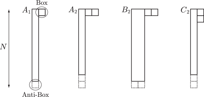
Figure 1: Simpler representations allowed in MQM.

The partition function becomes nontrivial after the restriction of the representation,

$$Z(q)=\sum_{R}d_{R}Z^{(R)}(q)\,,$$ (15)

where the summation over $R$ is for the admissible representation of $U(N)$, $d_{R}$ is the dimension of the representation and $Z^{(R)}(q)$ is the generating function of the multiplicity of the representation at level $n$ as the coefficient of $q^{n}$. For simpler representations, they are explicitly written as [3],

$$Z^{(S)}(q) =\prod_{n=1}^{N}\frac{1}{(1-q^{n})}\,,\quad Z^{(R)}(q)=P^{(R)}(q)Z^{(S)}(q)\,,$$ (16)

$$P^{(A_{1})}=\frac{q-q^{N}}{1-q}\,,\quad P^{(B_{2})}=\frac{q^{2}(1-q^{N-1})(1-q^{N})}{(1-q)(1-q^{2})},\quad P^{(C_{2})}=\frac{q^{2}(1-q^{N-3})(1-q^{N})}{(1-q)(1-q^{2})},$$

$$P^{(A_{2})}=\frac{q^{3}(1-q^{N-2})(1-q^{N-1})}{(1-q)(1-q^{2})}\,,$$ (17)

$$d_{B_{2}}=\frac{N^{2}(N+3)(N-1)}{4} ,\quad d_{C_{2}}=\frac{N^{2}(N-3)(N+1)}{4}\,,\quad d_{A_{2}}=\frac{(N^{2}-1)(N^{2}-4)}{4}\,.$$ (18)

At this point, it is possible to write the strategy of our study more precisely.

1. We give a systematic derivation of the MQM Hilbert space with specific irreducible representations of $U(N)$. Our strategy is to find the states with the specific representation $\rho$ of $U(N)$ with the lowest ${\mathcal{H}}_{0}$ eigenvalue as the highest weight state of the ${\widehat{\mathcal{W}}}_{\infty}$ algebra. The generic states with the representation $\rho$ can be generated from this set of states by applying the ${\widehat{\mathcal{W}}}_{\infty}$ operators. It explains the decomposition (15) where $Z^{(R)}(q)$ are regarded as “characters” of the representations of ${\widehat{\mathcal{W}}}_{\infty}$.

2. As we noted, the diagonalization of the Hamiltonian is trivial in the creation/annihilation basis since it just counts the number of creation operators. These states are, however, not convenient for many purposes since they are not diagonal with respect to the inner product. As we will see, the ${\widehat{\mathcal{W}}}_{\infty}$ algebra contains the infinite set of commuting charges which include ${\mathcal{H}}_{0}$ as the simplest charge. These operators are also important since their existence supports the integrability of MQM in the non-singlet sectors. We will construct the basis of the Hilbert space which are the eigenvectors of these infinite set of charges.

2.2 ${\widehat{\mathcal{W}}}_{\infty}$ algebra

As we have defined in the introduction, the ${\widehat{\mathcal{W}}}_{\infty}$ algebra is generated by the operators of the form (7) which commute with $U(N)$ generators,

$$\left[J_{\Lambda},{\mathcal{O}}^{(\epsilon_{1}\cdots\epsilon_{n})}\right]=0\,.$$ (19)

Before we study some detail of the algebra, it is useful to summarize our nomenclature on this algebra. We first note that operators of the form (7) are eigenstates of ${\mathcal{H}}_{0}$, $\left[{\mathcal{H}}_{0},{\mathcal{O}}^{(\epsilon_{1}\cdots\epsilon_{n})}\right]=m{\mathcal{O}}^{(\epsilon_{1}\cdots\epsilon_{n})}\,,$ where $m$ is the number of $\bar{A}$ minus the number of $A$. We call this eigenvalue of ${\mathcal{O}}^{(\epsilon_{1}\cdots\epsilon_{n})}$ as the degree of this operator. Obviously by applying degree $n$ operator to level $m$ state produces a level $n+m$ state. Suppose we have a set of states $\{|a\rangle\}$ at level $n$ with some representation $\rho$ under $U(N)$ i.e. $J_{\Lambda}|a\rangle=\sum_{a}\rho_{ab}|b\rangle$. The commutativity (19) between $J_{\Lambda}$ and the ${\widehat{\mathcal{W}}}_{\infty}$ generator implies that ${\mathcal{O}}^{(\epsilon_{1}\cdots\epsilon_{n})}|a\rangle$ belongs to the same representation at level $n+m$ where $m$ is the degree of ${\mathcal{O}}^{(\epsilon_{1}\cdots\epsilon_{n})}$. Since the level is bounded from below, there must be a set of states $|R\rangle\!\rangle_{a}$ ($a=1,\cdots,\mathrm{dim}(R)$) which are annihilated by all the operators in ${\widehat{\mathcal{W}}}_{\infty}$ with negative degree. We call such set of states as the highest weight state (see footnote 3) of the ${\widehat{\mathcal{W}}}_{\infty}$ algebra for the representation $R$.

Here we should not confuse the highest weight conditions for $U(N)$ and ${\widehat{\mathcal{W}}}_{\infty}$. The former picks up one state in each set of states $\{|a\rangle\}$ which spans basis of the irreducible representation $\rho$. Such states exist at various levels. Partition functions which count such states are given as $Z^{(R)}(q)$. On the other hand, the latter condition picks up the representation space of $R$ with $d_{R}$ states at the lowest level.

It is also convenient to introduce the normal ordering prescription. As in the quantum field theory, we define the normal ordered operator ${:\!{\mathcal{O}}\!:}$ by putting all the annihilation operator $A$ on the right of creation operators $\bar{A}$. For example,

$${:\!{\mathcal{O}}^{+-+-}\!:}={:\!\mbox{Tr}(\bar{A}A\bar{A}A)\!:}=\sum_{i,j,k,l}\bar{A}_{ij}\bar{A}_{kl}A_{jk}A_{li}\,.$$ (20)

We note that the ordering of the matrix multiplication is not changed. By using normal ordered operator, one can avoid the unnecessary factors of order $N$ (and higher) in the operator algebra. It also makes it possible to recover the cyclicity in the trace, ${:\!\mbox{Tr}({\mathcal{O}}_{1}{\mathcal{O}}_{2})\!:}={:\!\mbox{Tr}({\mathcal{O}}_{2}{\mathcal{O}}_{1})\!:}$.

The algebra between the ${\widehat{\mathcal{W}}}_{\infty}$ generators are far more complicated than the usual ${\mathcal{W}}_{\infty}$ algebra and it seems not possible to write the whole algebra in a closed compact form. The complication comes in from the order dependence of operators and the inclusion of higher order differential operators. Instead of trying to write the whole algebra, we just present the algebra between a few simpler operators which contains a few $A$. It is enough to show some nontrivial features of the algebra. We define $J_{n}=\mbox{Tr}(\bar{A}^{n})$, $L_{n}=\mbox{Tr}(\bar{A}^{n+1}A)$ and $V_{n,m}={:\!\mbox{Tr}({\bar{A}^{n+1}A\bar{A}^{m+1}A})\!:}$. The commutation relations between these operators become,

$$[J_{n},J_{m}]=0\,,\quad[J_{n},L_{m}]=-nJ_{n+m}\,,\quad[L_{n},L_{m}]=(m-n)L_{n+m}\,,$$ (21)

$$\left[V_{n,m},J_{r}\right]=r\sum_{s=1}^{r-1}J_{n+s}J_{m+r-s}+2rL_{n+m+r}\,,$$ (22)

$$[V_{n,m},L_{r}]=2\sum_{s=0}^{r}V_{n+s,m+r-s}+\sum_{s=1}^{r}(r-s+1)(J_{m+s}L_{n+r-s}+J_{n+s}L_{m+r-s})$$

$$\hskip 62.0pt-(m+1)V_{n,m+r}-(n+1)V_{n+r,m}\,.$$ (23)

The algebra in the first line is identical with the usual $U(1)$ current algebra and Virasoro algebra without the central extension. It implies that we can keep some features of CFT even for the non-singlet sectors. The nonlinearity is a characteristic feature of the ${\widehat{\mathcal{W}}}_{\infty}$ algebra and it shows up in the algebra of $V_{n,m}$ in (22,23). In general, the ${\widehat{\mathcal{W}}}_{\infty}$ generators induce splitting and joining of the multi-trace operators as we will see in section 5. The above nonlinearities are simple examples of such property.

Finally, among the degree zero operators in ${\widehat{\mathcal{W}}}_{\infty}$, there are the infinite set of generators which commute with each other (the elements of Cartan sualgebra). We define,

$${H}_{n}={:\!\mbox{Tr }(\mathcal{L}^{n})\!:}\,,\qquad\mathcal{L}={\bar{A}A}\,,\quad n=1,2,3,\cdots\,.$$ (24)

In order to prove that they commute with each other, we use the commutation relation, $\left[{\mathcal{L}}_{rs},{\mathcal{L}}_{tu}\right]={\mathcal{L}}_{ru}\delta_{st}-{\mathcal{L}}_{ts}\delta_{ru}$. Commutation relations $\left[{\mathcal{L}}_{rs},H_{n}\right]=0$ and $\left[H_{n},H_{m}\right]=0$ follow from this algebra immediately. We note that this set of commuting generators contains the Hamiltonian ${\mathcal{H}}_{0}$ as the first generator $H_{1}$. We also remark that there are many other operators with degree zero in ${\widehat{\mathcal{W}}}_{\infty}$ such as $\mbox{Tr}(\bar{A}^{2}A^{2})$. These operators, however, do not commute with $H_{n}$ and can not be taken as elements of Cartan subalgebra.

2.3 Construction of non-singlet states by the ${\widehat{\mathcal{W}}}_{\infty}$ algebra

In the following, we give a few explicit constructions of the non-singlet sectors by using the ${\widehat{\mathcal{W}}}_{\infty}$ algebra. As we have explained, we first find the highest weight state of the ${\widehat{\mathcal{W}}}_{\infty}$ algebra which provide the non-singlet states at the lowest level. The generic non-singlet states can be generated from this highest weight vectors by applying the ${\widehat{\mathcal{W}}}_{\infty}$ generators with positive degree. In order to identify the irreducible set of states, it is convenient to re-order the product by using commutation relations to the following standard form,

$$\prod J_{s}\prod L_{r}\prod V_{n,m}\cdots|R\rangle\!\rangle\,.$$ (25)

Namely we reorder the operators which contains more $A$ to the right side of the operators with less $A$. In the following, we present the highest weight states at level 0,1,2.

Highest weight condition at level 0 and the singlet sector

There is only one state (Fock vacuum $|0\rangle$) and it automatically satisfies the highest weight state condition. Since $J_{\Lambda}|0\rangle=0$, this is the state which belongs to the singlet representation. Therefore, we write,

$$|S\rangle\!\rangle=|0\rangle\,.$$ (26)

It is clear that all the operators which contains $A$ annihilate $|S\rangle\!\rangle$. Therefore the generators which give rise to new states are limited to $J_{n}$ ($n=1,2,3,\cdots$). The general singlet state takes the form $P(J_{1},J_{2},\cdots)|S\rangle\!\rangle$ where $P$ is an arbitrary polynomial of $J_{1},J_{2},\cdots$. This is the Fock space of a free boson field or equivalently a free fermion field. It is consistent with the form of the partition function $Z^{(S)}(q)$ in (16). For the commuting charges $H_{n}$, the weights of $|S\rangle\!\rangle$ are

$${H_{m}}|S\rangle\!\rangle=0\;\;\;\;(m=1,2,3,\cdots).$$ (27)

Highest weight state at level 1 and the adjoint sector

At this level, there are $N^{2}$ states $\bar{A}_{ij}|0\rangle$. The only nontrivial highest weight condition is $\mbox{Tr}(A)|\mbox{state}\rangle={\mathcal{O}}^{(-)}|\mbox{state}\rangle=0$. The solutions to this condition are $N^{2}-1$ states,

$$|A_{1}\rangle\!\rangle_{ij}=(\bar{A}_{ij}-\frac{1}{N}\delta_{ij}\mbox{Tr}\bar{A})|0\rangle\,,\quad(i,j=1,\cdots,N)\,.$$ (28)

It is easy to see that $|A_{1}\rangle\!\rangle$ transforms as the adjoint representation,

$$J_{\Lambda}|A_{1}\rangle\!\rangle_{ij}=\sum_{k}\left(\Lambda_{ik}|A_{1}\rangle\!\rangle_{kj}-\Lambda_{kj}|A_{1}\rangle\!\rangle_{ik}\right)\,.$$ (29)

The remaining one state at level $1$ is a singlet state generated from $|S\rangle\!\rangle$. As we expected, the highest weight condition of ${\widehat{\mathcal{W}}}_{\infty}$ automatically picks up an irreducible representation of $U(N)$.

It is easy to see the operators which contain more than one $A$ annihilate $|A_{1}\rangle\!\rangle$. On the other hand applying $L_{n}$ generates a new state,

$$L_{n}\left(\bar{A}_{ij}-\frac{1}{N}\delta_{ij}\mbox{Tr}(\bar{A})\right)|0\rangle=\left((\bar{A}^{n+1})_{ij}-\frac{1}{N}\delta_{ij}\mbox{Tr}(\bar{A}^{n+1})\right)|0\rangle\,.$$ (30)

Applying $L_{n^{\prime}}$ further produces the state of the same form with different $n$. Then we apply $J_{n}$ to generate new states. The general states which belongs to the adjoint representation thus takes the form,

$$\left((\bar{A}^{n})_{ij}-\frac{1}{N}\delta_{ij}\mbox{Tr}(\bar{A}^{n})\right)P(J_{1},J_{2},\cdots)|0\rangle$$ (31)

with $n=1,2,\cdots$. It coincides with the claim of [7]. The number of states generated by (31) is given by the generating function

$$\left(\sum_{n=1}^{\infty}q^{n}\right)\prod_{n=1}^{\infty}\frac{1}{1-q^{n}}=\frac{q}{1-q}\prod_{n=1}^{\infty}\frac{1}{1-q^{n}}\,.$$ (32)

This is just the character in the adjoint sector. We note that all states which belong to the adjoint representation are created by the action of the ${\mathcal{W}}_{\infty}$ operators with the positive degree on the highest weight state (28). The eigenvalues of the highest weight states for $H_{n}$ are,

$${H_{1}}|A_{1}\rangle\!\rangle=|A_{1}\rangle\!\rangle\,,\quad{H_{n}}|A_{1}\rangle\!\rangle=0\,,(n>1)\,.$$ (33)

Highest weight state at level 2 and $B_{2}$ and $C_{2}$ sectors

Level 2 highest weight state is given by combining $\bar{A}_{ij}\bar{A}_{kl}$ with other terms where we take contractions of indices of this expression. Nontrivial constraints come from ${\mathcal{O}}^{(-)}$, ${\mathcal{O}}^{(+--)}$ and ${\mathcal{O}}^{(--)}$. Actually the third one does not produce independent constraint since $\left[{\mathcal{O}}^{(-)},{\mathcal{O}}^{(+--)}\right]={\mathcal{O}}^{(--)}$. We use,

$${\mathcal{O}}^{(-)}\bar{A}_{ij}\bar{A}_{kl}|0\rangle = \delta_{ij}\bar{A}_{kl}|0\rangle+\delta_{kl}\bar{A}_{ij}|0\rangle\,,$$ (34)

$${\mathcal{O}}^{(+--)}\bar{A}_{ij}\bar{A}_{kl}|0\rangle = \delta_{il}\bar{A}_{kj}|0\rangle+\delta_{kj}\bar{A}_{il}|0\rangle\,.$$ (35)

After some computation, we found combinations

$$|B_{2}\rangle\!\rangle_{ijkl} = \left[\bar{A}_{ij}\bar{A}_{kl}+\bar{A}_{il}\bar{A}_{kj}\right.$$ (36)

$$-\frac{1}{N+2}(\mathrm{Tr}\bar{A})\left(\delta_{ij}\bar{A}_{kl}+\delta_{kl}\bar{A}_{ij}+\delta_{il}\bar{A}_{kj}+\delta_{kj}\bar{A}_{il}\right)$$

$$-\frac{1}{N+2}\left(\delta_{ij}\bar{A}^{2}_{kl}+\delta_{kl}\bar{A}^{2}_{ij}+\delta_{il}\bar{A}^{2}_{kj}+\delta_{kj}\bar{A}^{2}_{il}\right)$$

$$\left.+\frac{\delta_{ij}\delta_{kl}+\delta_{il}\delta_{kj}}{(N+1)(N+2)}\left((\mathrm{Tr}(\bar{A}))^{2}+(\mathrm{Tr}(\bar{A}^{2}))\right)\right]|0\rangle,$$

$$|C_{2}\rangle\!\rangle_{ijkl} = \left[\bar{A}_{ij}\bar{A}_{kl}-\bar{A}_{il}\bar{A}_{kj}\right.$$ (37)

$$-\frac{1}{N+2}(\mathrm{Tr}\bar{A})\left(\delta_{ij}\bar{A}_{kl}+\delta_{kl}\bar{A}_{ij}-\delta_{il}\bar{A}_{kj}-\delta_{kj}\bar{A}_{il}\right)$$

$$+\frac{1}{N+2}\left(\delta_{ij}\bar{A}^{2}_{kl}+\delta_{kl}\bar{A}^{2}_{ij}-\delta_{il}\bar{A}^{2}_{kj}-\delta_{kj}\bar{A}^{2}_{il}\right)$$

$$\left.+\frac{\delta_{ij}\delta_{kl}-\delta_{il}\delta_{kj}}{(N+1)(N+2)}\left((\mathrm{Tr}(\bar{A}))^{2}-(\mathrm{Tr}(\bar{A}^{2}))\right)\right]|0\rangle\,,$$

satisfy the highest weight condition. The eigenvalues of $H_{n}$ for these states are,

$$H_{1}|B_{2},C_{2}\rangle\!\rangle=2|B_{2},C_{2}\rangle\!\rangle\,,\quad H_{2}|B_{2}\rangle\!\rangle=2|B_{2}\rangle\!\rangle\,,\quad H_{2}|C_{2}\rangle\!\rangle=-2|C_{2}\rangle\!\rangle\,,$$

$$H_{m}|B_{2},C_{2}\rangle\!\rangle=0\,,\quad(m>2)\,.$$ (38)

We note that $H_{2}$ eigenvalue distinguishes $|B_{2}\rangle\!\rangle$ and $|C_{2}\rangle\!\rangle$ which could not be separated by ${\mathcal{O}}^{(-)}$ and ${\mathcal{O}}^{(+--)}$ conditions alone.

For these states the application of $V_{n,m}$ becomes nontrivial. It produces the states of the form,

$$\left((\bar{A}^{n})_{ij}(\bar{A}^{m})_{kl}+(\bar{A}^{m})_{ij}(\bar{A}^{n})_{kl}\pm(\bar{A}^{n})_{il}(\bar{A}^{m})_{kj}\pm(\bar{A}^{n})_{kj}(\bar{A}^{m})_{il}+\cdots\right)|0\rangle$$ (39)

for $B_{2}$ (resp. $C_{2}$) representations. It is easy to check that applying $V_{n^{\prime},m^{\prime}}$ further, or $L_{n^{\prime}}$ does not produce new type of states. Since they are symmetric under $n\leftrightarrow m$, the number of the state which is generated from the first factor is given as,

$$\sum_{1\leq n\leq m}q^{n+m}=\frac{q^{2}}{(1-q)(1-q^{2})}\,.$$ (40)

This is exactly the prefactor $P^{(B_{2},C_{2})}(q)$ in (17) in the large $N$ limit. Finally we can multiply the state with any polynomials of $J_{n}$ as the singlet and the adjoint sectors. So the most general form of $B_{2}$ and $C_{2}$ representation sector has the form (39) multiplied by $P(J_{1},J_{2},\cdots)$.

We note that at level two, there are extra states, $2$ singlet states ($J_{1}^{2}|S\rangle\!\rangle$ and $J_{2}|S\rangle\!\rangle$), $2(N^{2}-1)$ states with adjoint representation ($J_{1}|A_{1}\rangle\!\rangle$ and $L_{1}|A_{1}\rangle\!\rangle$), and $d_{B_{2}},d_{C_{2}}$ states with $B_{2}$ and $C_{2}$ representation respectively. These span precisely the $N^{2}(N^{2}+1)/2$ dimensional level two states.

We have seen that the highest weight conditions of the ${\widehat{\mathcal{W}}}_{\infty}$ algebra are useful to obtain the explicit form of the wave functions in the non-singlet sectors. It is also clear that the number of the state at each level is given by the character of the ${\widehat{\mathcal{W}}}_{\infty}$ algebra. We do not have, however, the complete classification of the irreducible representations of ${\widehat{\mathcal{W}}}_{\infty}$ which should be classified according to the eigenvalues of $H_{n}$. This issue remains as an important open problem which should be solved as the ${\mathcal{W}}_{\infty}$ algebra [12, 13].

3 Calogero(-Sutherland)-type interaction in ${\widehat{\mathcal{W}}}_{\infty}$ generators

In the following chapters, we derive the exact spectrum of the commuting charges $H_{n}$ of the ${\widehat{\mathcal{W}}}_{\infty}$ algebra and their eigenstates. Usually, this problem is approached by reducing the dynamical degree of freedom to the eigenvalues of matrices $X$ and solve the Hamiltonian problem with the Calogero-type interaction (3). As we noted in the previous section, in the creation and annihilation basis, to find eigenfunction of the Hamiltonian is trivial since the Hamiltonian just counts the number of creation operators applied to the vacuum. Therefore a nontrivial issue is how to diagonalize higher charges $H_{n}$ ($n=2,3,4,\cdots$). In this section, we derive the explicit form of $H_{2}$ in terms of the eigenvalues of $\bar{A}$ and derive the interaction term which is similar to the Calogero-Sutherland interaction. We will solve the eigenvalue problem (for the adjoint sector) in the next section by applying the bosonization technique. The procedure in these sections illuminates the direct correspondence between the solvable system and CFT which generalizes the free fermion in the singlet sector.

Since $A$ and $\bar{A}$ are $q$-numbers, it will be more convenient to introduce $c$-number matrix $\bar{Z}$ as the eigenvalue of $\bar{A}$ in the coherent state basis,

$$\langle 0|e^{\mathrm{Tr}(A\bar{Z})}|\Psi\rangle=\Psi(\bar{Z})\,\,,\quad\bar{A}_{ij}|\Psi\rangle\rightarrow\bar{Z}_{ij}\Psi(\bar{Z})\,,\quad A_{ij}|\Psi\rangle\rightarrow\frac{\partial}{\partial\bar{Z}_{ji}}\Psi(\bar{Z})\,.$$ (41)

We diagonalize $\bar{Z}$ as $\bar{Z}=e^{K}\bar{z}e^{-K}$ where $\bar{z}$ is a diagonal matrix and $e^{K}$ ($K:$ anti-hermitian) is a unitary transformation which is needed for the diagonalization. We expand $\bar{Z}$ in terms of $K$,

$$\bar{Z}_{ij}=\bar{z}_{i}\delta_{ij}+(\bar{z}_{j}-\bar{z}_{i})K_{ij}+\frac{1}{2}\sum_{k}(\bar{z}_{i}+\bar{z}_{j}-2\bar{z}_{k})K_{ik}K_{kj}+\mathcal{O}(K^{3})\,.$$ (42)

$K$ will be put to be zero at the end of the computation. However, in order to express the differentiation with respect to the matrix $\bar{Z}$, we need to keep it for a while.

We determine the differentiation with respect to $\bar{A}$ by the requirement,

$$\frac{\partial}{\partial\bar{Z}_{ij}}\bar{Z}_{kl}=\delta_{ik}\delta_{jl}\,.$$ (43)

We write

$$\frac{\partial}{\partial\bar{Z}_{ij}}=\sum_{r}\mathcal{A}_{ij,r}\partial_{r}+\sum_{r,s}\mathcal{B}_{ij,rs}\frac{\partial}{\partial K_{sr}}$$ (44)

(with $\partial_{r}=\frac{\partial}{\partial\bar{z}_{r}}$) and expand the coefficients as

$$\mathcal{A}_{ij,r}=\mathcal{A}^{(0)}_{ij,r}+\mathcal{A}_{ij,r}^{(1)}+\mathcal{A}_{ij,r}^{(2)}\cdots\,,\quad\mathcal{B}_{ij,r}=\mathcal{B}^{(0)}_{ij,rs}+\mathcal{B}_{ij,rs}^{(1)}+\mathcal{B}_{ij,rs}^{(2)}\cdots\,,$$ (45)

where $\mathcal{A}^{(n)}$ and $\mathcal{B}^{(n)}$ are $\mathcal{O}(K^{n})$. We can fix these coefficients order by order by requiring (43). For example, the coefficients for ${\mathcal{O}}(1)$ and ${\mathcal{O}}(K)$ are,

$$\mathcal{A}^{(0)}_{ij,k}=\delta_{ij}\delta_{jk}\,,$$ (46)

$$\mathcal{B}^{(0)}_{ij,rs}=\frac{\delta_{ir}\delta_{js}(1-\delta_{rs})}{\bar{z}_{r}-\bar{z}_{s}}\,,$$ (47)

$$\mathcal{A}^{(1)}_{ij,k}=K_{ij}(\delta_{jk}-\delta_{ik})\,,$$ (48)

$$\mathcal{B}^{(1)}_{ij,lk}=\left(\frac{1-\delta_{kl}}{\bar{z}_{l}-\bar{z}_{k}}-\frac{1}{2}\frac{1-\delta_{ik}}{\bar{z}_{i}-\bar{z}_{k}}\right)\delta_{jk}K_{il}-\left(\frac{1-\delta_{kl}}{\bar{z}_{l}-\bar{z}_{k}}-\frac{1}{2}\frac{1-\delta_{ij}}{\bar{z}_{i}-\bar{z}_{j}}\right)\delta_{il}K_{kj}$$ (49)

It is equivalent to the expression,

$$\frac{\partial}{\partial\bar{Z}_{ij}} = \delta_{ij}\partial_{j}+\frac{1-\delta_{ij}}{\bar{z}_{i}-\bar{z}_{j}}\partial_{K_{ji}}+K_{ij}(\partial_{j}-\partial_{i})+\sum_{l}\left(\frac{1-\delta_{jl}}{\bar{z}_{l}-\bar{z}_{j}}-\frac{1}{2}\frac{1-\delta_{ij}}{\bar{z}_{i}-\bar{z}_{j}}\right)K_{il}\partial_{K_{lj}}$$ (50)

$$-\sum_{l}\left(\frac{1-\delta_{il}}{\bar{z}_{i}-\bar{z}_{l}}-\frac{1}{2}\frac{1-\delta_{ij}}{\bar{z}_{i}-\bar{z}_{j}}\right)K_{lj}\partial_{K_{li}}+\mathcal{O}(K^{2})\,.$$

These operators can be applied to the wave function with the representation $\rho$ through the $K$ dependence in $\Psi^{(\rho)}_{a}(\bar{Z})=\rho(e^{K})_{ab}\Psi^{(\rho)}_{b}(\bar{z})$. In order to see it more explicitly, we consider the adjoint representation in the following. The wave function becomes,

$$\Psi(\bar{Z})_{ij} = \left(e^{K}\Psi(\bar{z})e^{-K}\right)_{ij}$$ (51)

$$= \psi_{i}\delta_{ij}+(\psi_{j}-\psi_{i})K_{ij}+\frac{1}{2}\sum_{k}(\psi_{i}+\psi_{j}-2\psi_{k})K_{ik}K_{kj}+\cdots$$

where we denote the diagonal component of $\Psi(\bar{z})$ as $\psi_{i}(\bar{z})$. The expression for the higher charges in terms of the eigenvalues are given by writing the action of $\mbox{Tr }(\bar{Z}\frac{\partial}{\partial\bar{Z}})^{n}$ to $\Psi(\bar{Z})$ and putting $K=0$ at the end. We note that in the course of the computation we need higher $K$ dependent terms since we have differentiation with respect to $K$.

Since we have an explicit expression only to the first order in $K$, we can obtain only ${H}_{1}$ and $H_{2}$. The first one $H_{1}$ is trivial,

$$(H^{(A_{1})}_{1}\cdot\psi)_{k}=\sum_{i}{\bar{z}_{i}\partial_{i}}\psi_{k}\,.$$ (52)

We put a suffix $A_{1}$ in order to specify that this is the expression for the adjoint sector. The second one becomes,

$$(H^{(A_{1})}_{2}\cdot\psi)_{k}=\sum_{i}(\bar{z}_{i}\partial_{i})^{2}\psi_{k}-2\sum_{i(\neq k)}\frac{\bar{z}_{i}\bar{z}_{k}}{(\bar{z}_{k}-\bar{z}_{i})^{2}}(\psi_{k}-\psi_{i})$$

$$~{}~{}~{}-\sum_{i}(\bar{z}_{i}\partial_{i})\psi_{k}+\sum_{i\neq j}\left(\bar{z}_{i}\bar{z}_{j}\frac{1-\delta_{ij}}{\bar{z}_{i}-\bar{z}_{j}}(\partial_{i}-\partial_{j})\right)\psi_{k}$$ (53)

The first two terms give the Calogero-Sutherland Hamiltonian. The third term is proportional to $H_{1}$ and not relevant for the diagonalization. The fourth term is somewhat new. If we rewrite $\bar{z}_{i}=e^{\theta_{i}}$, the action of $H_{2}$ can be written as Calogero-Sutherland [16] like form,

$$(H^{(A_{1})}_{2}\psi)_{i} = \sum_{i}\frac{\partial^{2}\psi_{k}}{\partial\theta_{i}^{2}}-\sum_{i}\frac{\partial\psi_{k}}{\partial\theta_{i}}-\frac{1}{2}\sum_{i(\neq k)}\frac{\psi_{k}-\psi_{i}}{\mathrm{sinh}^{2}(\theta_{ik}/2)}$$ (54)

$$+\frac{1}{2}\sum_{i\neq j}\frac{1}{\sinh(\theta_{ij}/2)}\left(e^{-\theta_{ij}/2}\partial_{\theta_{i}}-e^{\theta_{ij}/2}\partial_{\theta_{j}}\right)\psi_{k},$$

where $\theta_{ij}=\theta_{i}-\theta_{j}$.

For the usual Calogero-Sutherland model, there have been a large number of references where Hamiltonian system analogous to (53) or (54) is solved directly in terms of $\bar{z}$ variables [17]. Here, rather than moving to this direction, we rewrite this Hamiltonian by bosonization technique and solve it from this approach [14].

4 Bosonization

In order to describe the non-singlet sectors in a way similar to the singlet sector, it is natural to introduce free boson variables,

$$p_{r}=\mbox{Tr }\bar{Z}^{r}=\sum_{i}\bar{z}^{r}_{i}\,,$$ (55)

(which is called “collective coordinate” or “power sum” in the literature) and rewrite the ${\widehat{\mathcal{W}}}_{\infty}$ operators in terms of $p_{r}$ and the degree of freedom associated with the tips. Free boson oscillators are usually defined as $\alpha_{n}=n\partial_{p_{n}}$, $\alpha^{\dagger}_{n}=p_{n}$ for $n>0$. They satisfy standard commutation relations,

$$\left[\alpha_{n},\alpha^{\dagger}_{m}\right]=n\delta_{n,m}\,.$$ (56)

In the following we focus on writing the explicit forms of the quantities $H_{1}$, $H_{2}$, $H_{3}$ when they are applied to specific (non-)singlet sectors. For simplicity we consider the singlet $(S)$, the adjoint $(A_{1})$, and $B_{2}$, $C_{2}$ representations. For each case, by the results of §2, the wave functions are written as the linear combinations of

$${S} : f(p_{1},p_{2},\cdots)\quad\Rightarrow\quad f(p)\,,$$

$${A_{1}} : ((\bar{Z}^{n})_{ij}+\cdots)f(p_{1},p_{2},\cdots)\quad\Rightarrow\quad f(p)|n\rangle\,,$$

$${B_{2}} : \left((\bar{Z}^{n})_{ij}(\bar{Z}^{m})_{kl}+(\bar{Z}^{m})_{ij}(\bar{Z}^{n})_{kl}+(\bar{Z}^{n})_{il}(\bar{Z}^{m})_{kj}+(\bar{Z}^{n})_{kj}(\bar{Z}^{m})_{il}+\cdots\right)f(p_{1},p_{2},\cdots)$$

$$\quad\Rightarrow\quad f(p)|n,m;+\rangle\,,$$

$${C_{2}} : \left((\bar{Z}^{n})_{ij}(\bar{Z}^{m})_{kl}+(\bar{Z}^{m})_{ij}(\bar{Z}^{n})_{kl}-(\bar{Z}^{n})_{il}(\bar{Z}^{m})_{kj}-(\bar{Z}^{n})_{kj}(\bar{Z}^{m})_{il}+\cdots\right)f(p_{1},p_{2},\cdots)$$ (57)

$$\quad\Rightarrow\quad f(p)|n,m;-\rangle\,.$$

Here we have skipped writing the subleading order terms since they are not relevant in the following computation. In order to keep the formulae as simple as possible, we will use short hand notations which are written after the arrow $\Rightarrow$. The states $|n\rangle$, $|n,m;\pm\rangle$ represent the degrees of the freedom associated with the tips. For $B_{2}$ and $C_{2}$, they are symmetric $|n,m;\pm\rangle=|m,n;\pm\rangle$.

There are two different paths to obtain a bosonic representation of $H_{n}$. One is to use the expressions in terms of the eigenvalues which are obtained in the previous section. This approach has a benefit in showing the explicit relation between the Calogero-Sutherland type interactions and their bosonized representations. Another approach is to work directly with the matrix variables. Both approaches give, of course, the same answer. Since the expressions in terms of the eigenvalues are getting more and more complicated for the higher charges and the higher representations, we will basically use the latter approach.

The computation itself is straightfoward. We apply $\bar{Z}$ representation of $H_{n}$

$$H_{1} = \sum_{i,j}\bar{Z}_{ij}\frac{\partial}{\partial\bar{Z}_{ij}}\,,\quad H_{2}=\sum_{i,j,k,l}\bar{Z}_{ij}\bar{Z}_{kl}\frac{\partial}{\partial\bar{Z}_{kj}}\frac{\partial}{\partial\bar{Z}_{il}}\,,$$

$$H_{3} = \sum_{i,j,k,l,n,m}\bar{Z}_{ij}\bar{Z}_{kl}\bar{Z}_{nm}\frac{\partial}{\partial\bar{Z}_{kj}}\frac{\partial}{\partial\bar{Z}_{nl}}\frac{\partial}{\partial\bar{Z}_{im}}\,,$$ (58)

to the states (57) and rewrite the results by using the multiplications and the derivations of $p_{r}$. The useful formulae are, for example,

$$\left[\frac{\partial}{\partial\bar{Z}_{ji}},({\bar{Z}}^{n})_{kl}\right]=\sum_{m=1}^{n}({\bar{Z}}^{m-1})_{kj}({\bar{Z}}^{n-m})_{il}\,,$$

$$\left[\frac{\partial}{\partial\bar{Z}_{ji}},(p_{k})^{n}\right]=nk({\bar{Z}}^{k-1})_{ij}(p_{k})^{n-1},\quad\left[\frac{\partial}{\partial\bar{Z}_{ji}},f(p)\right]=\sum_{r=1}^{N}r({\bar{Z}}^{r-1})_{ij}{\partial}_{p_{r}}f(p)\,.$$ (59)

After some computation, we arrive at the bosonized formulae for $H_{1}$,$H_{2}$, $H_{3}$.

The expressions for $H_{1}$ (Hamiltonian) are trivial as usual,

$$H^{(S)}_{1}f(p) = \left(\sum_{r}rp_{r}\partial_{p_{r}}\right)f(p)\,,$$ (60)

$$H^{(A_{1})}_{1}f(p)|n\rangle = \left(n+\sum_{r}rp_{r}\partial_{p_{r}}\right)f(p)|n\rangle\,,$$ (61)

$$H^{(B_{2},C_{2})}_{1}f(p)|n,m;\pm\rangle = \left(n+m+\sum_{r}rp_{r}\partial_{p_{r}}\right)f(p)|n,m;\pm\rangle\,.$$ (62)

Here and in the following, we use the upper sign for $B_{2}$ and the lower sign for $C_{2}$.

In the expressions for $H_{2}$, there appear various cross terms among the free bosons and the tips,

$${H^{(S)}_{2}}f(p) = \left(\sum_{r,s=1}^{N}rsp_{r+s}\partial_{p_{r}}\partial_{p_{s}}+\sum_{l=1}^{N}\sum_{r=1}^{l-1}lp_{r}p_{l-r}\partial_{p_{l}}\right)f(p)\,,$$ (63)

$${H^{(A_{1})}_{2}}f(p)|n\rangle = 2n\sum_{r=1}^{N}r\partial_{p_{r}}f(p)|n+r\rangle+2\sum_{s=1}^{n-1}(n-s)p_{s}f(p)|n-s\rangle\,,$$ (64)

$$+H_{2}^{(S)}f(p)|n\rangle\,,$$

$${H^{(B_{2},C_{2})}_{2}}f(p)|n,m;\pm\rangle = 2n\sum_{r=1}^{N}r\partial_{p_{r}}f(p)|n+r,m;\pm\rangle+2m\sum_{r=1}^{N}r\partial_{p_{r}}f(p)|n,m+r;\pm\rangle$$ (65)

$$+2\sum_{s=1}^{n-1}(n-s)p_{s}f(p)|n-s,m;\pm\rangle+2\sum_{s=1}^{m-1}(m-s)p_{s}f(p)|n,m-s;\pm\rangle$$

$$\pm 2\sum_{r=1}^{n}\sum_{s=1}^{m}f(p)|n-r+s,m+r-s;\pm\rangle+H_{2}^{(S)}f(p)|n,m;\pm\rangle\,.$$

Obviously $H_{2}^{(S)}$ describes the mixing among the free bosons. In the free fermion language, it reduces to $\oint\bar{\psi}(z)(z\partial_{z})^{2}\psi(z)$. This part is common in every sector. The first two terms in $H_{2}^{(A_{1})}$ and the first four terms in $H_{2}^{(B_{2},C_{2})}$ describe the mixing between the tip and the free boson. They have again the similar form in both $A_{1}$ and $B_{2},C_{2}$. Finally the fifth term in $H_{2}^{(B_{2},C_{2})}$ describes the mixing among the tips. We note the sign difference between $B_{2}$ and $C_{2}$. It is not difficult to confirm that these interactions take the similar forms for even higher representations.

These expressions can be written without the reference to the wave functions if we introduce the shift operators $\hat{E}_{p}$ as (for the adjoint sector)

$$\hat{E}_{p}|n\rangle=\left\{\begin{array}[]{c l}(n-p)|n-p\rangle&p<n\\ 0&p\geq n\end{array}\right.\,,\quad\hat{E}_{0}|n\rangle=n|n\rangle\,,\quad\hat{E}_{-p}|n\rangle=n|n+p\rangle\,.$$ (66)

Together with the free boson oscillator, the conserved charges are written as

$$H^{(A_{1})}_{1}=\hat{E}_{0}+H_{1}^{(S)}\,,\quad{H^{(A_{1})}_{2}}=2\sum_{r=1}^{N}\hat{E}_{-r}\alpha_{r}+2\sum_{s=1}^{N}\hat{E}_{s}\alpha^{\dagger}_{s}+H_{2}^{(S)}\,,$$ (67)

where

$$H^{(S)}_{1}=\sum_{r=1}^{N}\alpha^{\dagger}_{r}\alpha_{r}\,,\quad H_{2}^{(S)}=\sum_{r,s=1}^{N}\alpha^{\dagger}_{r+s}\alpha_{r}\alpha_{s}+\sum_{l=1}^{N}\sum_{r=1}^{l-1}\alpha^{\dagger}_{r}\alpha^{\dagger}_{l-r}\alpha_{l}\,.$$ (68)

Writing a similar formula for $B_{2}$ and $C_{2}$ is straightfoward.

The expression for $H_{3}$ becomes more complicated and we present only the expressions for the singlet and the adjoint sectors. The strategy of the computation is the same as before. The final result is, for the singlet sector,

$$\begin{split}&{H_{3}}^{(S)}f(p)=\sum_{r,s,t}rstp_{r+s+t}{\partial}_{p_{r}}{\partial}_{p_{s}}{\partial}_{p_{t}}f-\sum_{r,s}rsp_{r}p_{s}{\partial}_{p_{r}}{\partial}_{p_{s}}f\\ &~{}~{}~{}~{}~{}+\sum_{r,s}\left(\sum_{l=1}^{r+s-1}+\sum_{l=1}^{r-1}\right)rsp_{l}p_{r+s-l}{\partial}_{p_{r}}{\partial}_{p_{s}}f+\sum_{r}\sum_{l=1}^{r-1}\sum_{m=1}^{r-l-1}rp_{l}p_{m}p_{r-l-m}{\partial}_{p_{r}}f\\ &~{}~{}~{}~{}~{}+\frac{1}{2}\sum_{r}r(r-1)(r-2)p_{r}{\partial}_{p_{r}}f+\frac{1}{2}n(n-1)(n-2)f\,.\end{split}$$ (69)

The expression for the adjoint sector involves extra terms which describe the mixing between the bosons and the tip,

$$\begin{split}&{H_{3}}^{(A_{1})}f(p)|n\rangle=(H_{3}^{(S)}f(p))|n\rangle\\ &~{}~{}~{}~{}~{}+3n\sum_{r,s}rs{\partial}_{p_{r}}{\partial}_{p_{s}}f|n+r+s\rangle+3n\sum_{r}\sum_{l=1}^{r-1}rp_{l}{\partial}_{p_{r}}f|n+r-l\rangle\\ &~{}~{}~{}~{}~{}+3\sum_{r}\sum_{l=1}^{r-1}r(n-l)p_{l}{\partial}_{p_{r}}f|n+r-l\rangle+3\sum_{r}\sum_{l=1}^{n-1}r(n-l)p_{r+l}{\partial}_{p_{r}}f|n-l\rangle\\ &~{}~{}~{}~{}~{}+\sum_{l=1}^{n-1}\sum_{m=1}^{l-1}(n-l)p_{m}p_{l-m}f|n-l\rangle+\sum_{l=1}^{n}\sum_{m=1}^{l-1}\left(\sum_{k=1}^{l-m-1}+\sum_{k=1}^{n-l}\right)p_{m}p_{k}f|n-m-k\rangle\,.\end{split}$$ (70)

Numerical evaluation of the spectrum of $H_{2}$ and $H_{3}$

One of the important questions in this paper is to determine the spectrum of $H_{n}$ ($n=1,2,3,\cdots$) for the various sectors. For the singlet sector, the problem is already solved since it is the free fermion system. The eigenstate is labelled by Young diagram $Y$ which represents the spectrum of fermionic system through Maya diagram correspondence [18]. We write the fermionic state that corresponds to $Y$ as $|Y\rangle$. The eigenstate in terms of $p$ is written by using the boson-fermion correspondence

$$\langle 0|e^{\sum_{n=1}^{\infty}\frac{\alpha_{n}}{n}p_{n}}|Y\rangle=s_{Y}(p)$$ (71)

where $s_{Y}(p)$ is Schur polynomial in terms of the power sum. The eigenvalues of $H_{1,2}$ is given as,

$$h_{1}(Y)=\sum_{i}\mu_{i}=|Y|\,,\qquad h_{2}(Y)=\sum_{i=1}^{l}\mu_{i}(\mu_{i}-2i+1)$$ (72)

where $\mu_{i}$ is the number of boxes in $i$-th raw in $Y$($\mu_{1}\geq\mu_{2}\geq\cdots\geq\mu_{l}>0$). The eigenvalues of $H_{2}^{(S)}$ and their multiplicity are summarized in the following table. In the table, “level” means the eigenvalue of $H_{1}$. One can see that the most of the degeneracy of the spectrum at the level of the Hamiltonian ($H_{1}$) is resolved by considering $H_{2}$. Some eigenvalues have the multiplicity larger than one since different Young tableaux have the same values of $h_{2}$ accidentally. These degeneracies are resolved by considering $H_{3}$ and so on.

level	${H^{(S)}_{2}}$ eigenvalues (exponent is multiplicity)
0	0
1	0
2	$\pm 2$
3	$\pm 6$, $0$
4	$\pm 12$, $\pm 4$, $0$
5	$\pm 20$, $\pm 10$, $\pm 4$, $0$
6	$\pm 30$, $\pm 18$, $\pm 10$, $\pm 6^{2}$, $0$
7	$\pm 42$, $\pm 28$, $\pm 18$, $\pm 14$, $\pm 12$, $\pm 6$, $\pm 2$, $0$
8	$\pm 56$, $\pm 40$, $\pm 28$, $\pm 24$, $\pm 20$, $\pm 16$, $\pm 14$, $\pm 8^{2}$, $\pm 4$, $0^{2}$

For the adjoint sector (and also $B_{2}$ and $C_{2}$ sectors), it is still difficult for us to evaluate the spectrum in terms of the bosonization language. We will determine it from the different viewpoint in the next section. Here we present the result in advance to explain the important feature of the spectrum of the non-singlet sector. It is, of course, possible to perform a direct computer calcuation based on (61) and (64) (actually this is what we did before we found the analytic solution). These analysis are, of course, consistent with each other.

The spectrum of $H_{2}^{(A_{1})}$ is shown by the following table.

level	${H^{(A_{1})}_{2}}$ eigenvalues (exponent is multiplicity)
1	0
2	$\pm 2$
3	$\pm 6$, $0^{2}$
4	$\pm 12$, $\pm 4^{2}$, $0$
5	$\pm 20$, $\pm 10^{2}$, $\pm 4^{2}$, $0^{2}$
6	$\pm 30$, $\pm 18^{2}$, $\pm 10^{2}$, $\pm 6^{3}$, $0^{3}$
7	$\pm 42$, $\pm 28^{2}$, $\pm 18^{2}$, $\pm 14^{2}$, $\pm 12^{2}$, $\pm 6^{3}$, $\pm 2^{2}$, $0^{2}$
8	$\pm 56$, $\pm 40^{2}$, $\pm 28^{2}$, $\pm 24^{2}$, $\pm 20^{2}$, $\pm 16$, $\pm 14^{3}$, $\pm 8^{5}$, $\pm 4^{2}$, $0^{5}$

Interestingly, the eigenvalues are precisely identical with the singlet sector (72) up to the multiplicity! It is surprising that the extra terms in $H^{(A_{1})}_{2}$ associated with the “tip” does not change the spectrum.

It may be a natural guess that the degeneracy appearing $H_{2}$ in the adjoint sector can be removed if we consider higher conserved charges such as $H_{3},H_{4}\ldots$. However this is not the case. The following table shows the eigenvalues of $H_{3}^{(A_{1})}$ and their multiplicity computed from (70).

level	${H^{(A_{1})}_{3}}$ eigenvalues (exponent is multiplicity)
1	$0$
2	$0^{2}$
3	$6^{2}$, $-3^{2}$
4	$24^{2}$, $0^{4}$, $-12$
5	$60^{2}$, $15^{4}$, $0^{2}$, $-12^{4}$
6	$120^{2}$, $48^{4}$, $12^{4}$, $0^{4}$, $-15^{3}$, $-24^{2}$
7	$210^{2}$, $105^{2}$, $42^{4}$, $30^{4}$, $21^{2}$, $-6^{6}$, $-15^{4}$, $-30^{4}$
8	$336^{2}$, $192^{4}$, $96^{4}$, $84^{4}$, $48^{4}$, $21^{6}$, $12^{4}$, $0^{3}$, $-24^{12}$, $-48^{2}$

These eigenvalues are identical to the exact spectrum $h_{3}(Y)$ which we derive later (95). We note that the multiplicity is even larger than that of $H_{2}^{(A_{1})}$ because the eigenvalues $h_{3}(Y)$ have additional degeneracy for the states associated with different Young diagrams. It resolves, however, some accidental degeneracy in $H_{2}$. For example, the Young diagrams $[4,1,1]$ and $[3,3]$ have the same $h_{2}(Y)$ but different $h_{3}(Y)$,

$$h_{2}([4,1,1])=h_{2}([3,3])=6,\;\;h_{3}([4,1,1])=12,\;\;h_{3}([3,3])=-24.$$ (73)

The most important degeneracy due to the location of the “tip” remain.

5 Group theoretical construction of eigenstates of $H_{n}$

5.1 Analogy with matrix string theory

In the previous section, we have seen that the spectrum of $H_{2}$ (and also $H_{3}$) for the adjoint sector is identical to that for the singlet sector. This feature actually remains the same for any non-singlet sectors. We will show this fact by explicit construction of their eigenstates. It turns out that the problem can be solved by an application of the group theory at the relatively elementary level.

We first develop a compact notation to represent generic states in the MQM Hilbert space. We note that a state of the form $\bar{A}_{i_{1}j_{1}}\cdots\bar{A}_{i_{n}j_{n}}|0\rangle$ can be written as a single trace operator acting on the Fock vacuum, $\operatorname{Tr}({\mathcal{C}}_{1}\bar{A}\cdots{\mathcal{C}}_{n}\bar{A})|0\rangle$ with $({\mathcal{C}}_{1})_{ij}=\delta_{ij_{n}}\delta_{ji_{1}}$, $({\mathcal{C}}_{2})_{ij}=\delta_{ij_{1}}\delta_{ji_{2}}$ and so on. It is clear that arbitrary states can be written as the sum of such single trace form with more general constant ${\mathcal{C}}$. In order to describe more generic state, it is more useful to introduce the multi-trace operators, $\prod_{I=1}^{P}\mbox{Tr }({\mathcal{C}}^{(I)}_{1}\bar{A}\cdots{\mathcal{C}}^{(I)}_{n_{I}}\bar{A})|0\rangle\,.$

With this notation, the wave function in the singlet sector can be represented by a linear combination of such operator with ${\mathcal{C}}=1$. To represent the adjoint state, we put one of ${\mathcal{C}}$’s as a traceless tensor and other ${\mathcal{C}}$ to be identity. For $B_{2}$ and $C_{2}$, we keep two of ${\mathcal{C}}$’s arbitrary with the appropriate symmetry properties.

We apply $H_{2}$ to such multi-trace operator state, the an interesting structure shows up,

$$\frac{1}{2}{H_{2}}\prod_{I=1}^{P}\mbox{Tr }({\mathcal{C}}^{(I)}_{1}\bar{A}\cdots{\mathcal{C}}^{(I)}_{n_{I}}\bar{A})|0\rangle$$

$$~{}=\sum_{J=1}^{P}\left(\prod_{I(\neq J)}^{P}\mbox{Tr }({\mathcal{C}}^{(I)}_{1}\bar{A}\cdots{\mathcal{C}}^{(I)}_{n_{I}}\bar{A})\right)\cdot$$

$$~{}~{}~{}\cdot\sum_{1\leq i<j\leq n_{J}}\mbox{Tr}\left({\mathcal{C}}^{(J)}_{i+1}\bar{A}\cdots{\mathcal{C}}^{(J)}_{j}\bar{A}\right)\mbox{Tr }\left({\mathcal{C}}^{(J)}_{1}\bar{A}\cdots{\mathcal{C}}^{(J)}_{i}\bar{A}{\mathcal{C}}^{(J)}_{j+1}\bar{A}\cdots{\mathcal{C}}^{(J)}_{n_{J}}\bar{A}\right)|0\rangle$$

$$~{}~{}~{}~{}+\sum_{J<K}\left(\prod_{I(\neq J,K)}^{P}\mbox{Tr }({\mathcal{C}}^{(I)}_{1}\bar{A}\cdots{\mathcal{C}}^{(I)}_{n_{I}}\bar{A})\right)\cdot$$ (74)

$$~{}~{}~{}~{}\cdot\sum_{i,j}\mbox{Tr}\left({\mathcal{C}}^{(J)}_{1}\bar{A}\cdots{\mathcal{C}}^{(J)}_{i}\bar{A}{\mathcal{C}}^{(K)}_{j+1}\bar{A}\cdots{\mathcal{C}}^{(K)}_{n_{K}}\bar{A}{\mathcal{C}}^{(K)}_{1}\bar{A}\cdots{\mathcal{C}}^{(K)}_{j}\bar{A}{\mathcal{C}}^{(J)}_{i+1}\bar{A}\cdots{\mathcal{C}}^{(J)}_{n_{J}}\bar{A}\right)|0\rangle\,.$$

If we regard each single trace operator as a “loop operator”, the action of $H_{2}$ represents splitting and joining of such operators (fig. 2).

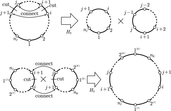
Figure 2: Splitting and joining rules of $H_{2}$. Each loop represents a single trace operator.

This is an intriguing feature of $H_{2}$ which have an interpretation in terms of the string field theory. For example in the matrix string theory, such a splitting and joining interaction among the long strings is triggered by the permutation of the short strings. In our case, the long string is given by the matrix ${\mathcal{C}}\bar{A}$ and the short string replaced by the single trace operator. This analogy gives us a hope that the action of $H_{2}$ may have similar structure as the matrix string theory[15]. This is indeed the case.

We have a similar representation for $H_{3}$. In order to simplify the notation, we introduce

$${\mathcal{A}}_{ij}=\left\{\begin{array}[]{ll}{\mathcal{C}}_{i}{\bar{A}}{\mathcal{C}}_{i+1}{\bar{A}}\cdots{\mathcal{C}}_{j}{\bar{A}}&\mbox{for }i<j\\ {\mathcal{C}}_{i}{\bar{A}}\cdots{\mathcal{C}}_{n}{\bar{A}}{\mathcal{C}}_{1}{\bar{A}}\cdots{\mathcal{C}}_{j}{\bar{A}}&\mbox{for }i>j\,.\end{array}\right.$$ (75)

which describe a portion of the trace operator $\mbox{Tr}({\mathcal{C}}_{1}{\bar{A}}\cdots{\mathcal{C}}_{n}{\bar{A}})$. The action of $H_{3}$ is written as

$$\begin{split}&\frac{1}{3}H_{3}\prod_{I=1}^{P}\mbox{Tr}({\mathcal{A}}_{1n_{I}}^{(I)})|0\rangle=\\ &\sum_{J=1}^{P}\left(\prod_{I(\neq J)}\mbox{Tr}({\mathcal{A}}_{1n_{I}}^{(I)})\right)\sum_{1\leq i<j<k\leq n_{J}}\Bigl{[}\mbox{Tr}({\mathcal{A}}_{i+1,j}^{(J)}{\mathcal{A}}_{k+1,i}^{(J)}{\mathcal{A}}_{j+1,k}^{(J)})+\mbox{Tr}({\mathcal{A}}_{i+1,j}^{(J)})\mbox{Tr}({\mathcal{A}}_{j+1,k}^{(J)})\mbox{Tr}({\mathcal{A}}_{k+1,i}^{(J)})\Bigr{]}|0\rangle\\ +&\sum_{J<K}\left(\prod_{I(\neq J,K)}\mbox{Tr}({\mathcal{A}}_{1n_{I}}^{(I)})\right)\sum_{\begin{subarray}{c}1\leq i<j\leq n_{J}\\ 1\leq k\leq n_{K}\end{subarray}}\Bigl{[}\mbox{Tr}({\mathcal{A}}_{i+1,j}^{(J)}{\mathcal{A}}_{k+1,k}^{(K)})\mbox{Tr}({\mathcal{A}}_{j+1,i}^{(J)})+\mbox{Tr}({\mathcal{A}}_{j+1,i}^{(J)}{\mathcal{A}}_{k+1,k}^{(K)})\mbox{Tr}({\mathcal{A}}_{i+1,j}^{(J)})\Bigr{]}|0\rangle\\ +&2\sum_{J<K<L}\left(\prod_{I(\neq J,K,L)}\mbox{Tr}({\mathcal{A}}_{1n_{I}}^{(I)})\right)\sum_{\begin{subarray}{c}1\leq i\leq n_{J}\\ 1\leq j\leq n_{K}\\ 1\leq k\leq n_{L}\end{subarray}}\mbox{Tr}({\mathcal{A}}_{i+1,i}^{(J)}{\mathcal{A}}_{j+1,j}^{(K)}{\mathcal{A}}_{k+1,k}^{(L)})|0\rangle.\end{split}$$ (76)

It describes splitting and joining processes of $3\rightarrow 1$, $2\rightarrow 2$, $1\rightarrow 3$ between the loops. Clearly one can continue to carry out this type of the computation for higher $H_{n}$.

5.2 Exact eigenstates in terms of Young symmetrizer

In the matrix string theory, the interaction between the loops can be given by the permutation of the connection between the string bits. In the following we will see that exactly the same type of the representation exists for $H_{n}$ and it enables us to construct the exact eigenstate by using a group theoretical method.

For this purpose, we introduce an economical notation of the multi-trace operators by using the action of the permutation group $S_{n}$,

$$\Psi(\left\{{\mathcal{C}}\right\};\sigma)=\sum_{a_{1},\cdots,a_{n}}({\mathcal{C}}_{1}\bar{A})_{a_{1}a_{\sigma(1)}}\cdots({\mathcal{C}}_{n}\bar{A})_{a_{n}a_{\sigma(n)}}|0\rangle\,.$$ (77)

Here $\sigma$ is an element of $S_{n}$. We note that a similar representation for the singlet state apeared in [19]. The structure of the multi-trace operator comes from the decomposition of $\sigma\in S_{n}$ as a product of cycles,

$$\sigma=(a_{1}a_{2}\cdots a_{\mu_{1}})(b_{1}b_{2}\cdots b_{\mu_{2}})\cdots\,,$$ (78)

where $(a_{1}a_{2}\cdots a_{\mu_{1}})$ represents a cyclic permutation, i.e. $\sigma(a_{1})=a_{2},\cdots,\sigma(a_{\mu_{1}})=a_{1}$. The corresponding $\Psi(\left\{{\mathcal{C}}\right\};\sigma)$ is written as the product of the loop operators,

$$\Psi(\left\{{\mathcal{C}}\right\};\sigma)=\mbox{Tr}({\mathcal{C}}_{a_{1}}\bar{A}\cdots{\mathcal{C}}_{a_{\mu_{1}}}\bar{A})\mbox{Tr}({\mathcal{C}}_{b_{1}}\bar{A}\cdots{\mathcal{C}}_{b_{\mu_{2}}}\bar{A})\cdots|0\rangle.$$ (79)

A direct computation shows that the operator $H_{2}$ can be represented as the sum of permutation operators,

$${H_{2}}\Psi(\left\{{\mathcal{C}}\right\};\sigma)=\sum_{i\neq j}\Psi(\left\{{\mathcal{C}}\right\};{\sigma(ij)})\,.$$ (80)

As we claimed, this is the interaction of the matrix string theory [15] where the string bits are replaced by the matrices ${\mathcal{C}}_{i}\bar{A}$. More generally it is not difficult to show that the action of $H_{m}$ takes a similar form,

$${H_{m}}\Psi(\left\{{\mathcal{C}}\right\};\sigma)=\sum_{i_{1},\cdots,i_{m}\,(i_{a}\neq i_{b})}\Psi(\left\{{\mathcal{C}}\right\};{\sigma(i_{1}i_{2}\cdots i_{m})})\,,$$ (81)

where the summation is taken for the set of mutually different integers $i_{1},\cdots,i_{m}$. At this point, it becomes straightfoward to construct eigenvectors of $H_{m}$ by means of the group theory. Let us define the action of $\tau\in S_{n}$ on $\Psi(\sigma)$ as the left multiplication,

$$\rho(\tau)\Psi(\left\{{\mathcal{C}}\right\};\sigma)=\Psi(\left\{{\mathcal{C}}\right\};\tau\sigma)\,.$$ (82)

Then it is clear that this action commute with $H_{m}$,

$$\rho(\tau){H_{m}}\Psi(\left\{{\mathcal{C}}\right\};\sigma)={H_{m}}\rho(\tau)\Psi(\left\{{\mathcal{C}}\right\};\sigma)=\sum_{i_{1}\cdots i_{m}}\Psi(\left\{{\mathcal{C}}\right\};\tau\sigma(i_{1}\cdots i_{m}))\,.$$ (83)

It is then possible to use Young symmetrizer [20] associated with a board $B_{Y}$ of a Young diagram $Y$ to obtain an eigenstate. The Young symmetrizer in general is written as,

$$e_{B_{Y}}=\frac{d_{Y}}{n!}a_{B_{Y}}b_{B_{Y}},$$ (84)

where

$$a_{B_{Y}}=\sum_{\sigma\in H_{B_{Y}}}\rho(\sigma)\,,\quad b_{B_{Y}}=\sum_{\sigma\in R_{B_{Y}}}(-1)^{\sigma}\rho(\sigma)\,.$$ (85)

Here $d_{Y}$ is the dimension of the irreducible representation of $S_{n}$ associated with diagram $Y$ and $H_{B_{Y}}$ (resp. $R_{B_{Y}}$) is the horizontal (resp. vertical) permutation associated with the board $B_{Y}$. Since $e_{B_{Y}}$ is a projector ($e_{B_{Y}}^{2}=e_{B_{Y}}$), it defines a projection of Hilbert space into lower dimensional subspace. We claim that the states after this projection

$$\Psi^{[B_{Y}]}=e_{B_{Y}}\Psi(\left\{{\mathcal{C}}\right\};\sigma)\,,\quad(\sigma\in S_{n})$$ (86)

become the eigenfunctions for $H_{1}$, $H_{2}$ and $H_{3}$,

$$H_{1}\Psi^{[B_{Y}]}=h_{1}(Y)\Psi^{[B_{Y}]}\,,\quad H_{2}\Psi^{[B_{Y}]}=h_{2}(Y)\Psi^{[B_{Y}]}\,,\quad H_{3}\Psi^{[B_{Y}]}=h_{3}(Y)\Psi^{[B_{Y}]}\,,$$ (87)

where $h_{1}(Y)$ and $h_{2}(Y)$ are defined in (72) and $h_{3}(Y)$ will be given in (95). A proof of this statement is given in the next subsection and it seems natural to conjecture that one may straightforwardly generalize it for all $H_{n}$.

The simplicity of the form of the exact eigenstate (86) is remarkable. We will refer the eigenstate constructed in this way as Young symmetrizer state (YSS).

We note that there are some freedom in YSS (86), namely the choice of the constant matrices ${\mathcal{C}}$, the choice of the board $B_{Y}$ for each Young diagram $Y$ and the choice of $\sigma$. It explains the origin of the degeneracy of the spectrum in the non-singlet sectors. We note that the eigenvalue depends only on the Young diagram $Y$.

Of course, the different choices does not always produce independent states. For example, the choice of the board can be absorbed in the choice of the constant matrices ${\mathcal{C}}$ assigned in each box in $Y$. Furthermore, the different assignments of ${\mathcal{C}}$ sometimes produce an identical state as we see later in the adjoint sector. The locations of the matrices ${\mathcal{C}}\,(\neq 1)$ should be interpreted as the locations of the “tips” in the spectrum of the background fermion.

5.3 Calculation of the eigenvalues

In this subsection, we give a detailed proof of (87) for $H_{2}$ and $H_{3}$. Proof for $H_{1}$ is trivial.

$H_{2}$:

We compute the action of $H_{2}$ on YSS as,

$$H_{2}\Psi^{[B_{Y}]}=\frac{d_{Y}}{n!}\sum_{i\neq j}\Psi(a_{B_{Y}}b_{B_{Y}}\sigma(ij))=\frac{d_{Y}}{n!}\sum_{i\neq j}\Psi(a_{B_{Y}}(ij)b_{B_{Y}}\sigma)\,.$$ (88)

We can evaluate the action of transposition $(ij)$ according to the following rule.

• When the boxes $i$ and $j$ belong to the same row, $a_{B_{Y}}(ij)=a_{B_{Y}}$. Therefore it has eigenvalue $+1$. There are $\sum_{i}\mu_{i}(\mu_{i}-1)$ such pairs where $\mu_{i}$ is the length of $i$-th row.

• When the boxes $i$ and $j$ belong to the same column, $(ij)b_{B_{Y}}=-b_{B_{Y}}$. Therefore it has eigenvalue $-1$. There are $\sum_{i}\mu^{\prime}_{i}(\mu^{\prime}_{i}-1)$ such pairs where $\mu^{\prime}_{i}$ is the length of $i$-th column.

• When the boxes $i$ and $j$ do not meet with above two conditions, $a_{B_{Y}}(ij)b_{B_{Y}}=0$. It can be shown as follows. Let $k$ be the box which belongs to the same row with $i$ and the same column with $j$ (or vice versa),

  $$a_{B_{Y}}(ij)b_{B_{Y}}=a_{B_{Y}}\frac{1+(ik)}{2}(ij)\frac{1-(jk)}{2}b_{B_{Y}}=0\,.$$ (89)

The eigenvalue of $H_{2}$ becomes

$$\sum_{i}\mu_{i}(\mu_{i}-1)-\sum_{i}\mu^{\prime}_{i}(\mu^{\prime}_{i}-1)=\left(\sum_{i}\mu_{i}(\mu_{i}-2i+1)\right)=\mu_{2}(Y)\,.$$ (90)

$H_{3}$:

As $H_{2}$, we use the representation of $H_{3}$ as the sum of permutation operators:

$$H_{3}\Psi(\sigma)=\sum_{i\neq j\neq k\neq i}\Psi(\sigma(ijk))\,.$$ (91)

The action of $H_{3}$ on YSS (86) becomes

$$H_{3}\Psi^{[B]}=\frac{d_{Y}}{n!}\sum_{i\neq j\neq k\neq i}\Psi(a_{B}b_{B}\sigma(ijk))=\frac{d_{Y}}{n!}\sum_{i\neq j\neq k\neq i}\Psi(a_{B}(ijk)b_{B}\sigma)\,.$$ (92)

The non-vanishing contributions to the eigenvalue come from the following three cases:

• The boxes $i,j,$ and $k$ belong to the same row. In this case, since $a_{B}(ijk)=a_{B}$, the contribution is $\sum_{i}\mu_{i}(\mu_{i}-1)(\mu_{i}-2)\Psi^{[B]}$.

• The boxes $i,j,$ and $k$ belong to the same column. In this case, since $(ijk)b_{B}=b_{B}$, the contribution is $\sum_{i}\mu_{i}^{\prime}(\mu_{i}^{\prime}-1)(\mu_{i}^{\prime}-2)\Psi^{[B]}$.

• Two boxes (e.g. $i$ and $j$) belong to the same row, and two boxes (e.g. $j$ and $k$) belong to the same column. In this case, since $(ijk)=(ij)(jk),\,a_{B}(ij)=a_{B}$ and $(jk)b_{B}=-b_{B}$, the contribution is $-3\sum_{i,j}(\mu_{i}-1)(\mu_{j}^{\prime}-1)\Psi^{[B]}$.

Except for above three cases, the contribution of $(ijk)$ to the eigenvalue vanishes. The reason is as follows. Three boxes do not belong to the same row nor the same column, so we can choose two boxes that belong to different rows and columns. We call these two boxes $i$ and $j$. Let $l$ be the box which belongs to the same row with $j$ and the same column with $i$. $l$ is not $k$ otherwise it becomes above third case. Therefore

$$a_{B}(ijk)b_{B}=a_{B}\frac{1+(jl)}{2}(ji)(jk)\frac{1-(il)}{2}b_{B}=a_{B}\frac{1+(jl)}{2}(ji)\frac{1-(il)}{2}(jk)b_{B}=0\,.$$ (93)

Finally (92) becomes

$$H_{3}\Psi^{[B]}=h_{3}(Y)\Psi^{[B]}\,,$$ (94)

where

$$h_{3}(Y)=\sum_{i}\mu_{i}(\mu_{i}-1)(\mu_{i}-2)+\sum_{i}\mu_{i}^{\prime}(\mu_{i}^{\prime}-1)(\mu_{i}^{\prime}-2)-3\sum_{i,j}(\mu_{i}-1)(\mu_{j}^{\prime}-1).$$ (95)

It seems to be natural to conjecture that generalizations of this type of the proof are possible and YSS is the eigenstate for higher $H_{n}$ ($n=4,5,\cdots$).

5.4 Explicit forms of the exact eigenstates in terms of free boson

The expression of the eigenfunctions (86) as YSS is simple, explicit and exact. However, in order to compare it with the result of CFT, it is not the most convenient form. In the following, we present our partial result to express YSS in the singlet and the adjoint sector in terms of the free boson (or fermion) oscillator and the degree of freedom associated with the tip.

In order to extract the eigenstate for a specific representation, we restrict the matrices ${\mathcal{C}}$ to a specific form. For example in order to obtain the singlet state, we put all ${\mathcal{C}}$ to be identity. To obtain the adjoint state, we put one of ${\mathcal{C}}$ to be a generic traceless matrix and all the other to be identity. In the appendix B, we present the explicit form of the wave function by the Young symmetrizer (86) for the lower levels. It will be useful to understand the basic feature of YSS and the discussion in this subsection.

The singlet sector

For the singlet sector, it is not difficult to prove that YSS is identical to the Schur polynomial. To see that, we first observe that the wave function $\Psi^{[B_{Y}]}$ is unique for each Young diagram since we need to put all ${\mathcal{C}}$ to be $1$. Since $\Psi^{[B_{Y}]}$ and the Schur polynomial $s_{Y}(J_{n})|0\rangle$ are both the eigenstates of the conserved charges $H_{1},H_{2},\cdots$ with the same eigenvalue and the multiplicity , it implies $\Psi^{[B_{Y}]}\propto s_{Y}(J_{n})|0\rangle$. The normalization is fixed by comparing the coefficient of one particular term, for example, $J_{1}^{n}|0\rangle$. In $\Psi^{[B_{Y}]}$, it comes from the term which is proportional to $e$ in the symmetrizer and is identical to $d_{Y}/n!$. On the other hand in the Schur polynomial, it is known to be $d_{Y}/n!$ again (from the Murnaghan-Nakayama rule) [21]. We conclude,

$$\Psi^{[B_{Y}]}|_{{\mathcal{C}}=1}=s_{Y}(J_{n})|0\rangle\,.$$ (96)

This is an interesting relation between the Schur polynomial and the Young symmetrizer. One can understand this fact by reminding that the Young symmetrizer is the projection to the irreducible representation when it acts on the tensor product of the fundamental representations [22]. In our case, since the state $\Psi^{[B_{Y}]}|_{{\mathcal{C}}=1}$ is given as the trace of the representation space associated with $Y$, it equals to the Schur polynomial, which is the character of $U(N)$.

The adjoint sector

In this case, the wave function $\Psi^{[B_{Y}]}$ depends only the location of the box in the Young diagram $Y$ where the associated matrix ${\mathcal{C}}$ is not $1$. There are naively $|Y|$ choices of such boxes. However, the number of the independent states are fewer than that. The multiplicity of eigenstates of $H_{2}$ for each Young diagram in the adjoint sector can reproduced by the following rule. We represent the Young diagram $Y$ in the form $[\mu_{1}^{r_{1}},\mu_{2}^{r_{2}},\cdots,\mu_{s}^{r_{s}}]$ ($\mu_{1}>\mu_{2}>\cdots>\mu_{s}>0$). Namely $Y$ is constructed by piling $s$ rectangles with size $\mu_{i}\times r_{i}$ vertically. The multiplicity for this Young diagram is the same as the number of the rectangles, namely $s$. It is identical to the number of the special boxes in $Y$ where $Y$ becomes another Young diagram $Y^{\prime}$ after one removes one of these boxes. Such boxes are located at the right-bottom corner of each rectangle (fig. 3).

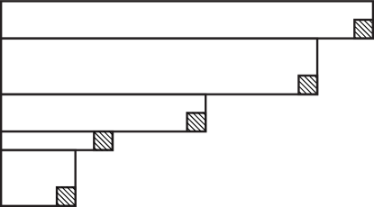
Figure 3: The multiplicity for each Young diagram in the adjoint sector equals to the number of boxes at the right-bottom corner of each rectangle.

This rule is also consitent with the partition function. For the singlet states, it is written as (one state for each Young diagram)

$$\sum_{r_{1},r_{2},\cdots=0}^{\infty}q^{\sum_{s=1}^{\infty}sr_{s}}=\prod_{n=1}^{\infty}\frac{1}{1-q^{n}}=Z^{(S)}(q)\,.$$ (97)

Here each set of integers $r_{n}$ represents a Young diagram which consists of the rectangles with sizes $n\times r_{n}$. In order to count the number of the adjoint state in the above rule, we multiply the number of rectangles $m([r])=\sum_{n=1}^{\infty}(1-\delta_{r_{n},0})$ in the summation over $r_{1},r_{2}\cdots$. It is then straightforward to show that

$$\sum_{r_{1},r_{2},\cdots=0}^{\infty}m([r])q^{\sum_{s=1}^{\infty}sr_{s}}=(q+q^{2}+q^{3}+\cdots)\prod_{n=1}^{\infty}\frac{1}{1-q^{n}}=\frac{q}{1-q}\prod_{n=1}^{\infty}\frac{1}{1-q^{n}}$$ (98)

which is exactly the partition function for the adjoint representation $Z^{(A_{1})}(q)$. Physically our observation here implies that the tips in the non-singlet sector do not affect the spectrum for any $H_{n}$ but only change the multiplicity through the freedom in their locations in the Young diagram.

From the explicit computation of the eigenfunction by the computer, it seems rather reasonable to conjecture that all the adjoint eigenstates can be written by the combinations of the (skew) Schur polynomials and the degree of freedom associated with the tip. So far it seems difficult to write them in compact forms. Therefore, we instead present the explicit forms of eigenstates for the Young diagrams with the limited shape.

For the diagrams $Y=[n],[1^{n}]$ the wave functions are simply given by

$$\Psi^{[n]}=\frac{1}{n}\sum_{r=0}^{n-1}\mbox{Tr}({\mathcal{C}}{\bar{A}}^{n-r})s_{[r]}(J)|0\rangle\,,\quad\Psi^{[1^{n}]}=\frac{1}{n}\sum_{r=0}^{n-1}(-1)^{n-r-1}\mbox{Tr}({\mathcal{C}}{\bar{A}}^{n-r})s_{[1^{r}]}(J)|0\rangle\,.$$ (99)

This is a situation where only one fermion (or hole) is excited and it is coupled with the tip.

Next we give the wave functions corresponding to $Y=[m,1^{n-1}]$. Naively, there are three independent boards but as we argued only two of them are independent. Considering the board shown in fig. 4 and putting ${\mathcal{C}}_{1}={\mathcal{C}}$, we obtain

$$\Psi^{[m,1^{n-1}]}_{1} =\frac{d_{[m,1^{n-1}]}}{(m+n-1)!}\sum_{\begin{subarray}{c}0\leq r\leq m-1\\ 0\leq s\leq n-1\end{subarray}}(-1)^{s}\operatorname{Tr}({\mathcal{C}}{\bar{A}}^{r+s+1})\frac{(m-1)!}{(m-r-1)!}\frac{(n-1)!}{(n-s-1)!}$$

$$\hskip 120.0pt\cdot(m-r-1)!s_{[m-r-1]}\cdot(n-s-1)!s_{[1^{n-s-1}]}|0\rangle$$

$$=\frac{1}{m+n-1}\sum_{\begin{subarray}{c}0\leq r\leq m-1\\ 0\leq s\leq n-1\end{subarray}}(-1)^{s}\operatorname{Tr}({\mathcal{C}}{\bar{A}}^{r+s+1})s_{[m-r-1]}s_{[1^{n-s-1}]}|0\rangle.$$ (100)

The coefficient of $\operatorname{Tr}({\mathcal{C}}{\bar{A}}^{r+s+1})$ comes from the number to choose $r$ boxes (considered their order) from $2,\dots,m$ and $s$ boxes from $m+1,\dots,m+n-1$ and from the product of the singlet states with remaining $Y=[m-r-1]$ and $[1^{n-s-1}]$. Other two states are similarly given by

$$\Psi^{[m,1^{n-1}]}_{2}=\frac{1}{(m+n-1)(m-1)} \biggl{[}\sum_{0\leq r\leq m-2}(m+n-r-2)\operatorname{Tr}({\mathcal{C}}{\bar{A}}^{r+1})s_{[m-r-1,1^{n-1}]}$$

$$+\sum_{\begin{subarray}{c}0\leq r\leq m-2\\ 0\leq s\leq n-1\end{subarray}}(-1)^{s}(r+1)\operatorname{Tr}({\mathcal{C}}{\bar{A}}^{r+s+2})s_{[m-r-2]}s_{[1^{n-s-1}]}\biggr{]}|0\rangle\,,$$ (101)

$$\Psi^{[m,1^{n-1}]}_{3}=\frac{1}{(m+n-1)(n-1)} \biggl{[}\sum_{0\leq s\leq n-2}(-1)^{s}(m+n-s-2)\operatorname{Tr}({\mathcal{C}}{\bar{A}}^{s+1})s_{[m,1^{n-s-2}]}$$

$$+\sum_{\begin{subarray}{c}0\leq r\leq m-1\\ 0\leq s\leq n-2\end{subarray}}(-1)^{s+1}(s+1)\operatorname{Tr}({\mathcal{C}}{\bar{A}}^{r+s+2})s_{[m-r-1]}s_{[1^{n-s-2}]}\biggr{]}|0\rangle\,,$$ (102)

where $\Psi^{[m,1^{n-1}]}_{2}$ is the state corresponding to ${\mathcal{C}}_{m}={\mathcal{C}}$ and $\Psi^{[m,1^{n-1}]}_{2}$ is that corresponding to ${\mathcal{C}}_{m+n-1}={\mathcal{C}}$. In (101) the first term comes from the case that the boxes 1 and $m$ are not in the same cyclic permutation, and the second term comes from the case that both are in the same one. The relation among these three states is as follows:

$$(m+n-2)\Psi^{[m,1^{n-1}]}_{1}-(m-1)\Psi^{[m,1^{n-1}]}_{2}-(n-1)\Psi^{[m,1^{n-1}]}_{3}=0\,.$$ (103)

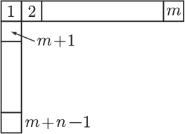
Figure 4: One board with the Young tableau $[m,1^{n-1}]$.

6 Summary and future issues

In this paper, we have studied the spectrum of MQM from the viewpoint of its spectrum generating algebra — the ${\widehat{\mathcal{W}}}_{\infty}$ algebra. While the usual ${\mathcal{W}}_{\infty}$ algebra is essentially described by free fermion systems [12, 13], ${\widehat{\mathcal{W}}}_{\infty}$ describes systems with Calogero(-Sutherland) type interaction which comes from the angular part of the matrix degree of freedom. The action of the ${\widehat{\mathcal{W}}}_{\infty}$ generators has an interpretation of the splitting and the joining of “loop operators” and through this interpretation it is possible to derive the explicit for of the eigenvectors for arbitrary non-singlet states. It is remarkable that the eigenfunctions of the commuting charges are still classified by the Young diagram and have the same spectrum as the free fermion system. The only difference is the degeneracy of the spectrum whose origin is the arbitrariness of the location of the tips.

There are a few questions which should be answered before we can study the issues of the non-singlet sectors of $c=1$ gravity. One important aspect is how to take large $N$ limit. While the representation in terms of the free boson and the degree of the freedom of the tip is a good framework to take the large $N$ analysis, our exact wave functions are defined through the Young symmetrizer and the translation between the two languages seems not complete in the non-singlet sector.

Another issue is how to solve the upside-down (UD) case. This is in a sense obtained from the upside-up (UU) case by a sort of Wick rotation. For instance, the wave function for the singlet sector is the Slater determinant of the free wave functions $x^{i\epsilon-1/2}$ (for UD case) instead of $x^{n}$ (for UU case). In order to consider the matrix generalization, we need to introduce the pure imaginary powers for the matrix $X$. We note that the basic tools of our analysis, the ${\widehat{\mathcal{W}}}_{\infty}$ generators, the Young symmetrizer and the free boson variables are defined in terms of the integer power of $X$. It is clear that we need extra ideas to modify our arguments to UD case. We hope that the basic observation of our analysis, the structure of the spectrum and the multiplicity will remain the same since it is a demonstration of the fact that the spectrum remains the same when we change the locations of the tips.

In the mathematical side, one important question is the study of the representation of the ${\widehat{\mathcal{W}}}_{\infty}$ algebra. While we discuss some simple irreducible representations which appear in the context of MQM, it should be far from the complete classification of the irreducible representations. The fact that the action of the generators takes the form of splitting and joining of loop operators implies that this algebra will be also essential to understand string theory beyond $c=1$.

Acknowledgement: This work was started as a joint project with I. Kostov. We are deeply grateful to him for the illuminating discussions and for his hospitality when Y.M. was invited to Saclay. Y.M. is supported in part by Grant-in-Aid (#16540232) from the Japan Ministry of Education, Culture, Sports, Science and Technology.

Appendix A Analogy with 3D harmonic oscillator

MQM in the nontrivial representation has many characters which are analogous to 3D harmonic oscillator with the Hamiltonian,

$$\mathcal{H}=-\frac{1}{2}\sum_{i=1}^{3}\frac{\partial^{2}}{\partial x_{i}^{2}}+\frac{1}{2}\sum_{i}x_{i}^{2}=\sum_{i=1}^{3}a_{i}^{\dagger}a_{i}+\frac{3}{2}$$ (104)

with

$$a_{i}=\frac{1}{\sqrt{2}}(x_{i}+ip_{i})=\frac{1}{\sqrt{2}}(x_{i}+\partial_{i})\,,\quad a^{\dagger}_{i}=\frac{1}{\sqrt{2}}(x_{i}-ip_{i})=\frac{1}{\sqrt{2}}(x_{i}-\partial_{i})\,.$$ (105)

In the polar coordinate, the Hamiltonian is rewritten as,

$$\mathcal{H}=-\frac{1}{2}\left(\frac{1}{r}\frac{\partial^{2}}{\partial r^{2}}r+\frac{1}{r^{2}}\hat{\Omega}\right)+\frac{1}{2}r^{2}\,,\quad\hat{\Omega}=\frac{1}{\sin\theta}\frac{\partial}{\partial\theta}\left(\sin\theta\frac{\partial}{\partial\theta}\right)+\frac{1}{\sin^{2}\theta}\frac{\partial^{2}}{\partial\phi^{2}}\,.$$ (106)

If we write the wave function as $\psi=R(r)Y_{lm}(\theta,\phi)$, the Schrödinger equation for $R(r)$ becomes,

$$-\frac{1}{2}\left(\frac{1}{r}\frac{\partial^{2}(rR)}{\partial r^{2}}\right)+\frac{1}{2}\left(r^{2}+\frac{l(l+1)}{r^{2}}\right)R(r)=ER(r)$$ (107)

The correspondence between MQM and 3D harmonic oscillator are, $A^{\pm}\leftrightarrow a_{i},a_{i}^{\dagger}$, the eigenvalues of $X\leftrightarrow r$, $U(N)$ rotation $\leftrightarrow SO(3)$, representation of $U(N)$ $\leftrightarrow$ total angular momentum $l$, $\sum_{i,j}\frac{\rho(E_{ij})\rho(E_{ji})}{(x_{i}-x_{j})^{2}}\leftrightarrow\frac{l(l+1)}{r^{2}}$ and so on.

The symmetry of the system is $SO(3)$ rotation generated by

$$L_{i}=i\epsilon_{ijk}x_{j}\partial_{k}=i\epsilon_{ijk}a^{\dagger}_{i}a_{j}$$ (108)

which commutes with the Hamiltonian. There is another $SL(2)$ algebra which commutes with $L_{i}$,

$$Q^{-}=\frac{1}{2}\sum_{i}(a_{i}^{\dagger})^{2},\quad Q^{0}=\frac{1}{2}(\sum_{i}a_{i}^{\dagger}a_{i}+\frac{3}{2})=\frac{1}{2}\mathcal{H},\quad Q^{+}=\frac{1}{2}\sum_{i}(a_{i})^{2}.$$ (109)

which satisfy the $sl(2,R)$ algebra,

$$\left[Q^{+},Q^{-}\right]=2Q^{0},\quad\left[Q^{0},Q^{\pm}\right]=\mp Q^{\pm}\,.$$ (110)

This is an analogue of ${\widehat{\mathcal{W}}}_{\infty}$. There is a relation between Casimir operator of $so(3)$ and $sl(2,R)$ generators,

$$\sum_{i=1}^{3}L_{i}^{2}=-4Q^{-}Q^{+}+(2Q^{0}-\frac{3}{2})(2Q^{0}-\frac{1}{2})=-4Q^{-}Q^{+}+(\mathcal{H}-\frac{3}{2})(\mathcal{H}-\frac{1}{2})$$ (111)

The shift appearing in $Q^{0}$ is due to the ground state energy of the harmonic oscillators. An analogue of this relation should exist for MQM which describes the correspondence between the representations of $U(N)$ and ${\widehat{\mathcal{W}}}_{\infty}$. So far, since we do not have a full understanding of the representation of ${\widehat{\mathcal{W}}}_{\infty}$, it is difficult to guess such relation.

The Hilbert space of the system is generated by the direct product of the irreducible representations of $so(3)$ ($L_{i}$) and $sl(2,R)$ ($Q^{\pm},Q^{0}$). For the $so(3)$ algebra, we have spin $l$ representation, $|l,m\rangle$ ($m=-l,-l+1,\cdots,l-1,l$). From this state, we generate irrep of $sl(2,R)$ algebra as

$$|n,l,m\rangle\!\rangle\propto(Q^{-})^{n}|l,m\rangle\!\rangle\,,\quad Q^{+}|l,m\rangle\!\rangle=0\,,\quad Q^{0}|l,m\rangle\!\rangle=\frac{1}{2}(l+\frac{3}{2})|l,m\rangle\!\rangle\,.$$ (112)

We have changed notation $|l,m\rangle\rightarrow|l,m\rangle\!\rangle$ since they are the ground state of $sl(2,R)$. The assignment of the weight is necessary since we have to impose,

$$L^{2}|l,m\rangle\!\rangle=l(l+1)|l,m\rangle\!\rangle=(2Q^{0}-\frac{3}{2})(2Q^{0}-\frac{1}{2})|l,m\rangle\!\rangle\,.$$ (113)

The state $|n,l,m\rangle\!\rangle$ ($n=0,1,2,\cdots$, $l=0,1,2\cdots$, $m=-l,\cdots,l$) span the Hilbert space of the system.

For example, the lower states are given as follows,

level $0$ $\displaystyle:$ $\displaystyle|0\rangle\leftrightarrow|0,0\rangle\!\rangle\,,$

level $$1 : a_{i}^{\dagger}|0\rangle\leftrightarrow|1,m\rangle\!\rangle\,,$$

level $$2 : a_{i}^{\dagger}a_{j}^{\dagger}|0\rangle\leftrightarrow|2,m\rangle\!\rangle\,,\,Q^{-}|0,0\rangle\!\rangle$$

level $$3 : a_{i}^{\dagger}a_{j}^{\dagger}a_{k}^{\dagger}|0\rangle\leftrightarrow|3,m\rangle\!\rangle\,,\,Q^{-}|1,m\rangle\!\rangle$$ (114)

The partition function associated with spin $l$ have the form, $(2l+1)q^{l+3/2}\frac{1}{1-q^{2}}$ where $(2l+1)$ is the number of state of spin $l$ representation, $l+3/2$ is the “ground state energy” for spin $l$ and $\frac{1}{1-q^{2}}$ is the partition function of $sl(2,R)$ representation. The total partition function is

$$\mbox{Tr}q^{\mathcal{H}-3/2}=\sum_{l=0}^{\infty}(2l+1)q^{l}\frac{1}{1-q^{2}}=\frac{1}{(1-q)^{3}}\,.$$ (115)

The right hand side is the partition function of three harmonic oscillators.

Appendix B Explicit form of the states constructed from Young symmetrizer at the lower levels

In order to see the relation between the states constructed from the Young symmetrizer and free boson (fermion) states, we present the explicit forms of the former at the lower levels.

Level 2

When $n=2$, the Young symmetrizers are, $e_{[2]}=\frac{1}{2}(1+(12))$, $e_{[1,1]}=\frac{1}{2}(1-(12))$ and the states that corresponds to them are

$$\Psi^{[2],[1^{2}]}=\frac{1}{2}\left(\mbox{Tr}({\mathcal{C}}_{1}\bar{A})\mbox{Tr}({\mathcal{C}}_{2}\bar{A})\pm\mbox{Tr}({\mathcal{C}}_{1}\bar{A}{\mathcal{C}}_{2}\bar{A})\right)|0\rangle\,.$$ (116)

The eigenvalue of $H_{2}$ is $\pm 2$ for $\Psi^{[2]}$ ($\Psi^{[1^{2}]}$). By restricting ${\mathcal{C}}_{1}={\mathcal{C}}_{2}=1$, $\Psi^{[Y]}$ reduces to Schur polynomial,

$$\Psi^{[2]} \rightarrow\frac{1}{2}(J_{1}^{2}+J_{2})|0\rangle=s_{[2]}(J)|0\rangle\,,\quad\Psi^{[1^{2}]}\rightarrow\frac{1}{2}(J_{1}^{2}-J_{2})|0\rangle=s_{[1^{2}]}(J)|0\rangle\,.$$ (117)

As for the restriction to the adjoint sector, with traceless matrix ${\mathcal{C}}$,

$$\Psi^{[2]}\rightarrow\frac{1}{2}(J_{1}\mbox{Tr}({\mathcal{C}}\bar{A})+\mbox{Tr}({\mathcal{C}}\bar{A}^{2}))|0\rangle\,,\qquad\Psi^{[1^{2}]}\rightarrow\frac{1}{2}(J_{1}\mbox{Tr}({\mathcal{C}}\bar{A})-\mbox{Tr}({\mathcal{C}}\bar{A}^{2}))|0\rangle$$ (118)

Level 3

Young symmetrizers are,

$$e_{[3]}=\frac{1}{3!}(1+(123)+(213)+(12)+(13)+(23))\,,$$ (119)

$$e_{[1^{3}]}=\frac{1}{3!}(1+(123)+(213)-(12)-(13)-(23))\,,$$ (120)

$$e_{[2,1]}=\frac{1}{3}(1+(12)-(13)-(123))\,.$$ (121)

There are several independent boards associated with $Y=[2,1]$. Here we pick up the following one:

From these projectors, one obtains the eigenstates of $H_{2}$ as,

$$\Psi^{[3]}=\frac{1}{3!}\left(\mbox{Tr}({\mathcal{C}}_{1}\bar{A})\mbox{Tr}({\mathcal{C}}_{2}\bar{A})\mbox{Tr}({\mathcal{C}}_{3}\bar{A})+\mbox{Tr}({\mathcal{C}}_{1}\bar{A}{\mathcal{C}}_{2}\bar{A}{\mathcal{C}}_{3}\bar{A})+\mbox{Tr}({\mathcal{C}}_{2}\bar{A}{\mathcal{C}}_{1}\bar{A}{\mathcal{C}}_{3}\bar{A})\right.$$

$$~{}~{}~{}\left.+\mbox{Tr}({\mathcal{C}}_{1}\bar{A}{\mathcal{C}}_{2}\bar{A})\mbox{Tr}({\mathcal{C}}_{3}\bar{A})+\mbox{Tr}({\mathcal{C}}_{1}\bar{A}{\mathcal{C}}_{3}\bar{A})\mbox{Tr}({\mathcal{C}}_{2}\bar{A})+\mbox{Tr}({\mathcal{C}}_{2}\bar{A}{\mathcal{C}}_{3}\bar{A})\mbox{Tr}({\mathcal{C}}_{1}\bar{A})\right)|0\rangle\,,$$

$$\Psi^{[1^{3}]}=\frac{1}{3!}\left(\mbox{Tr}({\mathcal{C}}_{1}\bar{A})\mbox{Tr}({\mathcal{C}}_{2}\bar{A})\mbox{Tr}({\mathcal{C}}_{3}\bar{A})+\mbox{Tr}({\mathcal{C}}_{1}\bar{A}{\mathcal{C}}_{2}\bar{A}{\mathcal{C}}_{3}\bar{A})+\mbox{Tr}({\mathcal{C}}_{2}\bar{A}{\mathcal{C}}_{1}\bar{A}{\mathcal{C}}_{3}\bar{A})\right.$$

$$~{}~{}~{}\left.-\mbox{Tr}({\mathcal{C}}_{1}\bar{A}{\mathcal{C}}_{2}\bar{A})\mbox{Tr}({\mathcal{C}}_{3}\bar{A})-\mbox{Tr}({\mathcal{C}}_{1}\bar{A}{\mathcal{C}}_{3}\bar{A})\mbox{Tr}({\mathcal{C}}_{2}\bar{A})-\mbox{Tr}({\mathcal{C}}_{2}\bar{A}{\mathcal{C}}_{3}\bar{A})\mbox{Tr}({\mathcal{C}}_{1}\bar{A})\right)|0\rangle\,,$$

$$\Psi^{[2,1]}=\frac{1}{3}\left(\mbox{Tr}({\mathcal{C}}_{1}\bar{A})\mbox{Tr}({\mathcal{C}}_{2}\bar{A})\mbox{Tr}({\mathcal{C}}_{3}\bar{A})+\mbox{Tr}({\mathcal{C}}_{1}\bar{A}{\mathcal{C}}_{2}\bar{A})\mbox{Tr}({\mathcal{C}}_{3}\bar{A})\right.$$

$$~{}~{}~{}\left.-\mbox{Tr}({\mathcal{C}}_{1}\bar{A}{\mathcal{C}}_{3}\bar{A})\mbox{Tr}({\mathcal{C}}_{2}\bar{A})-\mbox{Tr}({\mathcal{C}}_{1}\bar{A}{\mathcal{C}}_{2}\bar{A}{\mathcal{C}}_{3}\bar{A})\right)|0\rangle\,,$$ (122)

with

$$H_{2}\Psi^{[3]}=6\Psi^{[3]}\,,\quad H_{2}\Psi^{[1^{3}]}=-6\Psi^{[1^{3}]}\,,\quad H_{2}\Psi^{[2,1]}=0\,.$$ (123)

As before, the restriction to the singlet gives the corresponding Schur polynomials. The restriction to the adjoint is also similar. One important lesson here is that there are two independent states which can be derived from $\Psi^{[2,1]}$. By putting $({\mathcal{C}}_{1},{\mathcal{C}}_{2},{\mathcal{C}}_{3})=({\mathcal{C}},1,1)$ and $({\mathcal{C}}_{1},{\mathcal{C}}_{2},{\mathcal{C}}_{3})=(1,{\mathcal{C}},1)$

$$\frac{1}{3}\left(\mbox{Tr}({\mathcal{C}}\bar{A})J_{1}^{2}-\mbox{Tr}({\mathcal{C}}\bar{A}^{3})\right)|0\rangle\,,\quad\frac{1}{3}\left(\mbox{Tr}({\mathcal{C}}\bar{A})J_{1}^{2}+\mbox{Tr}({\mathcal{C}}\bar{A}^{2})J_{1}-\mbox{Tr}({\mathcal{C}}\bar{A})J_{2}-\mbox{Tr}({\mathcal{C}}\bar{A}^{3})\right)|0\rangle\,.$$ (124)

It explains the degeneracy 2 of the adjoint sector for $Y=[2,1]$.

References

-
[1]
V. A. Kazakov and A. A. Migdal,
Nucl. Phys. B 311, 171 (1988);
For the double scaling limit of theory,
E. Brezin, V. A. Kazakov and A. B. Zamolodchikov, Nucl. Phys. B 338, 673 (1990);
G. Parisi, Phys. Lett. B 238, 209 (1990);
D. J. Gross and N. Miljkovic, Phys. Lett. B 238, 217 (1990);
P. H. Ginsparg and J. Zinn-Justin, Phys. Lett. B 240, 333 (1990);
For the recent developments, for example,
S. Y. Alexandrov, V. A. Kazakov and I. K. Kostov, Nucl. Phys. B 640, 119 (2002) [arXiv:hep-th/0205079]; Nucl. Phys. B 667, 90 (2003) [arXiv:hep-th/0302106]. - [2] D. J. Gross and I. Klebanov, Nucl. Phys. B 344, 475 (1990); Nucl. Phys. B 354, 459 (1991).
- [3] D. Boulatov and V. Kazakov, Int. J. Mod. Phys. A 8, 809 (1993) [arXiv:hep-th/0012228].
- [4] V. Kazakov, I. K. Kostov and D. Kutasov, Nucl. Phys. B 622, 141 (2002) [arXiv:hep-th/0101011].
- [5] J. M. Maldacena, JHEP 0509, 078 (2005) [Int. J. Geom. Meth. Mod. Phys. 3, 1 (2006)] [arXiv:hep-th/0503112]; see also D. Gaiotto, arXiv:hep-th/0503215; J. M. Maldacena and N. Seiberg, JHEP 0509, 077 (2005) [arXiv:hep-th/0506141].
- [6] L. Fidkowski, arXiv:hep-th/0506132.
- [7] G. Marchesini and E. Onofri, J. Math. Phys. 21, 1103 (1980).
- [8] A. Agarwal and A. P. Polychronakos, arXiv:hep-th/0602049
- [9] A. P. Polychronakos, arXiv:hep-th/0607033.
-
[10]
E. Witten,
Nucl. Phys. B 373, 187 (1992)
[arXiv:hep-th/9108004];
J. Avan and A. Jevicki, Mod. Phys. Lett. A 7, 357 (1992) [arXiv:hep-th/9111028];
H. Itoyama and Y. Matsuo, Phys. Lett. B 262, 233 (1991);
A. Mironov and A. Morozov, Phys. Lett. B 252, 47 (1990). -
[11]
For the other works related to the algebra, see for example,
D. B. Fairlie and C. K. Zachos, Phys. Lett. B 224, 101 (1989);
I. Bakas, Commun. Math. Phys. 134, 487 (1990);
A. Cappelli, C. A. Trugenberger and G. R. Zemba, Nucl. Phys. B 448, 470 (1995) [arXiv:hep-th/9502021]. -
[12]
V. Kac and A. Radul,
Commun. Math. Phys. 157, 429 (1993)
[arXiv:hep-th/9308153];
E. Frenkel, V. Kac, A. Radul and W. Q. Wang, Commun. Math. Phys. 170, 337 (1995) [arXiv:hep-th/9405121]. - [13] H. Awata, M. Fukuma, Y. Matsuo and S. Odake, Commun. Math. Phys. 172, 377 (1995) [arXiv:hep-th/9405093]; Prog. Theor. Phys. Suppl. 118, 343 (1995) [arXiv:hep-th/9408158].
- [14] H. Awata, Y. Matsuo, S. Odake and J. Shiraishi, Phys. Lett. B 347, 49 (1995) [arXiv:hep-th/9411053]; Nucl. Phys. B 449, 347 (1995) [arXiv:hep-th/9503043].
- [15] R. Dijkgraaf, E. P. Verlinde and H. L. Verlinde, Nucl. Phys. B 500, 43 (1997) [arXiv:hep-th/9703030].
-
[16]
F. Calogero,
J. Math. Phys. 10, 2197 (1969);
B. Sutherland, J. Math. Phys. 12, 251 (1971). - [17] J. A. Minahan and A. P. Polychronakos, Phys. Lett. B 302, 265 (1993) [arXiv:hep-th/9206046]; A. P. Polychronakos, Nucl. Phys. B 419, 553 (1994) [arXiv:hep-th/9310095].
- [18] See for example E. Date, M. Jimbo, M. Kashiwara and T. Miwa, “Transformation Groups For Soliton Equations,” preprint RIMS-394, published in Proc. RIMS Symp. on Nonlinear Integrable System (Kyoto, 1981), eds. M. Jimbo and T. Miwa (World Scientific, Singapore, 1983); see also the appendix in the second reference of [13].
- [19] S. Corley, A. Jevicki and S. Ramgoolam, Adv. Theor. Math. Phys. 5, 809 (2002) [arXiv:hep-th/0111222].
- [20] For example, H. Weyl, “The Classical Groups: Their Invariants and Representations,” (Princeton 1939) chap. 4.
- [21] For example, R. P. Stanley, “Enumerative Combinatorics,” (Vol.2) (Cambridge 1999) chap. 7.
- [22] For example, W. Fulton and J. Harris, “Representation Theory,” (Springer-Verlag).