hep-th/0607050

PUPT-2202

ITEP-TH-32/06

On D3-brane Potentials in Compactifications with Fluxes and Wrapped D-branes

Daniel Baumann,¹ Anatoly Dymarsky,¹ Igor R. Klebanov,¹ Juan Maldacena,² Liam McAllister,¹ and Arvind Murugan¹

¹Joseph Henry Laboratories, Princeton University, Princeton, NJ 08544 ²Institute for Advanced Study, Princeton, NJ 08540

We study the potential governing D3-brane motion in a warped throat region of a string compactification with internal fluxes and wrapped D-branes. If the Kähler moduli of the compact space are stabilized by nonperturbative effects, a D3-brane experiences a force due to its interaction with D-branes wrapping certain four-cycles. We compute this interaction, as a correction to the warped four-cycle volume, using explicit throat backgrounds in supergravity. This amounts to a closed-string channel computation of the loop corrections to the nonperturbative superpotential that stabilizes the volume. We demonstrate for warped conical spaces that the superpotential correction is given by the embedding equation specifying the wrapped four-cycle, in agreement with the general form proposed by Ganor. Our approach automatically provides a solution to the problem of defining a holomorphic gauge coupling on wrapped D7-branes in a background with D3-branes. Finally, our results have applications to cosmological inflation models in which the inflaton is modeled by a D3-brane moving in a warped throat.

1 Introduction

1.1 Motivation

Cosmological inflation [2] is a remarkable idea that provides a convincing explanation for the isotropy and homogeneity of the universe. In addition, the theory contains an elegant mechanism to account for the quantum origin of large scale structure. The observational evidence for inflation is strong and rapidly growing [3], and in the near future it will be possible to falsify a large fraction of existing models. This presents a remarkable opportunity for inflationary model-building, and it intensifies the need for a more fundamental description of inflation than current phenomenological models can provide.

In string theory, considerable effort has been devoted to this problem. One promising idea is the identification of the inflaton field with the internal coordinate of a mobile D3-brane, as in brane-antibrane inflation models [4, 5], in which a Coulombic interaction between the branes gives rise to the inflaton potential. At the same time, advances in string compactification [6, 7] (for reviews, see [8]) have enabled the construction of solutions in which all moduli are stabilized by a combination of internal fluxes and wrapped D-branes. This has led to the formulation of realistic and moderately explicit models in which the brane-antibrane pair is inserted into such a stabilized flux compactification [9, 10, 11]. Particularly in warped throat regions of the compact space, the force between the branes can be weak enough to allow for prolonged inflation. It is therefore interesting to study the detailed potential determining D3-brane motion in a warped throat region, such as the warped deformed conifold [12] or its ‘baryonic branch’ generalizations, the resolved warped deformed conifolds [13, 14]. In [14] it was observed that a mobile D3-brane in a resolved warped deformed conifold experiences a force even in the absence of an antibrane at the bottom of the throat. This makes [14] a possible alternative to the brane-antibrane scenario of [9]. The calculations in this paper are carried out in a region sufficiently far from the bottom of the throat that the metrics of [12, 13, 14] are well-approximated by the asymptotic warped conifold metric found in [15]. Therefore, our methods apply to both scenarios, as well as to their generalizations to other warped cones.

A truly satisfactory model of inflation in string theory should include a complete specification of a string compactification, together with a reliable computation of the resulting four-dimensional effective theory. While some models come close to this goal, very small corrections to the potential can spoil the delicate flatness conditions required for slow-roll inflation [16]. In particular, gravitational corrections typically induce inflaton masses of order the Hubble parameter $H$, which are fatal for slow-roll. String theory provides a framework for a systematic computation of these corrections, but so far it has rarely been possible, in practice, to compute all the relevant effects. However, there is no obstacle in principle, and one of our main goals in this work is to improve the status of this problem.

It is well-known that a D3-brane probe of a ‘no-scale’ compactification [6] with imaginary self-dual three-form fluxes experiences no force: gravitational attraction and Ramond-Ramond repulsion cancel, and the brane can sit at any point of the compact space with no energy cost. This no-force result is no longer true, in general, when the volume of the compactification is stabilized. The D-brane moduli space is lifted by the same nonperturbative effect that fixes the compactification volume. This has particular relevance for inflation models involving moving D-branes.

In the warped brane inflation model of Kachru et al. [9] it was established that the interaction potential of a brane-antibrane pair in a warped throat geometry is exceptionally flat, in the approximation that moduli-stabilization effects are neglected. However, incorporating these effects yielded a potential that generically was not flat enough for slow roll. That is, certain correction terms to the inflaton potential arising from the Kähler potential and from volume-inflaton mixing [9] could be computed in detail, and gave explicit inflaton masses of order $H$. One further mass term, arising from a one-loop correction to the volume-stabilizing nonperturbative superpotential, was shown to be present, but was not computed. The authors of [9] argued that in some small percentage of possible models, this one-loop mass term might take a value that approximately canceled the other inflaton mass terms and produced an overall potential suitable for slow-roll. This was a fine-tuning, but not an explicit one: lacking a concrete computation of the one-loop correction, it was not possible to specify fine-tuned microscopic parameters, such as fluxes, geometry, and brane locations, in such a way that the total mass term was known to be small. In this paper we give an explicit computation of this key, missing inflaton mass term for brane motion in general warped throat backgrounds. Applications of our results to issues in brane inflation will be discussed in a future paper [18].

1.2 Method

The inflaton mass problem described in [9] appears in any model of slow-roll inflation involving D3-branes moving in a stabilized flux compactification. Thus, it is necessary to search for a general method for computing the dependence of the nonperturbative superpotential on the D3-brane position. Ganor [19] studied this problem early on, and found that the correction to the superpotential is a section of a bundle called the ‘divisor bundle’, which has a zero at the four-cycle where the wrapped brane is located. The problem was addressed more explicitly by Berg, Haack, and Körs (BHK) [20], who computed the threshold corrections to gaugino condensate superpotentials in toroidal orientifolds. This gave a substantially complete potential for brane inflation models in such backgrounds. However, their approach involved a challenging open-string one-loop computation that is difficult to generalize to more complicated Calabi-Yau geometries and to backgrounds with flux and warping, such as the warped throat backgrounds relevant for a sizeable fraction of current models. Moreover, KKLT-type volume stabilization often proceeds via a superpotential generated by Euclidean D3-branes [23], not by gaugino condensation or other strong gauge dynamics. In this case the one-loop correction comes from an instanton fluctuation determinant, which has not been computed to date.

Following [24], we overcome these difficulties by viewing the correction to the mobile D3-brane potential as arising from a distortion, sourced by the D3-brane itself, of the background near the four-cycle responsible for the nonperturbative effect. This corrects the warped volume of the four-cycle, changing the magnitude of the nonperturbative effect. Specifically, we assume that the Kähler moduli are stabilized by nonperturbative effects, arising either from Euclidean D3-branes or from strong gauge dynamics (such as gaugino condensation) on D7-branes. In either case, the nonperturbative superpotential is associated with a particular four-cycle, and has exponential dependence on the warped volume of this cycle. Inclusion of a D3-brane in the compact space slightly modifies the supergravity background, changing the warped volume of the four-cycle and hence the gauge coupling in the D7-brane gauge theory. Due to gaugino condensation this in turn changes the superpotential of the four-dimensional effective theory. The result is an energy cost for the D3-brane that depends on its location.

This method may be viewed as a closed-string dual of the open-string computation of BHK [20]. In §4.2 we compute the correction for a toroidal compactification, where an explicit comparison is possible, and verify that the closed-string method exactly reproduces the result of [20]. We view this as a highly nontrivial check of the closed-string method.

Employing the closed-string perspective allows us to study the potential for a D3-brane in a warped throat region, such as the warped deformed conifold [12] or its generalizations [13, 14], glued into a flux compactification. This is a case of direct phenomenological interest. To model the four-cycle bearing the most relevant nonperturbative effect, we compute the change in the warped volume of a variety of holomorphic four-cycles, as a function of the D3-brane position. We find that most of the details of the geometry far from the throat region are irrelevant. Note that our method is applicable provided that the internal manifold has large volume.

The distortion produced by moving a D3-brane in a warped throat corresponds to a deformation of the gauge theory dual to the throat by expectation values of certain gauge-invariant operators [25]. Hence, it is possible, and convenient, to use methods and perspectives from the AdS/CFT correspondence [26] (see [27, 28] for reviews).

1.3 Outline

The organization of this paper is as follows. In §2 we recall the problem of determining the potential for a D3-brane in a stabilized flux compactification. We stress that a consistent computation must include a one-loop correction to the volume-stabilizing nonperturbative superpotential. In §3 we explain how this correction may be computed in supergravity, as a correction to the warped volume of each four-cycle producing a nonperturbative effect. We present the Green’s function method for determining the perturbation of the warp factor at the location of the four-cycle in §4. We argue that supersymmetric four-cycles provide a good model for the four-cycles producing nonperturbative effects in general compactifications, and in particular in warped throats. In §5 we compute in detail the corrected warped volumes of certain supersymmetric four-cycles in the singular conifold. We also give results for corrected volumes in some other asymptotically conical spaces. In §6 we give an explicit and physically intuitive solution to the ‘rho problem’ [20], i.e. the problem of defining a holomorphic volume modulus in a compactification with D3-branes. We also discuss the important possibility of model-dependent effects from the bulk of the compactification. We conclude in §7.

In Appendix A we present some facts about Green’s functions on conical geometries, as needed for the computation of §5. We relegate the technical details of our computation for warped conifolds to Appendix B. The equivalent calculation for $Y^{p,q}$ cones is presented in Appendix C.

2 D3-branes and Volume Stabilization

2.1 Nonperturbative Volume Stabilization

For realistic applications to cosmology and particle phenomenology, it is important to stabilize all the moduli. The flux-induced superpotential [29] stabilizes the dilaton and the complex structure moduli [6], but is independent of the Kähler moduli. However, nonperturbative terms in the superpotential do depend on the Kähler moduli, and hence can lead to their stabilization [7]. There are two sources for such effects:

1. Euclidean D3-branes wrapping a four-cycle in the Calabi-Yau [23].

2. Gaugino condensation or other strong gauge dynamics on a stack of $N_{D7}$ spacetime-filling D7-branes wrapping a four-cycle in the Calabi-Yau.

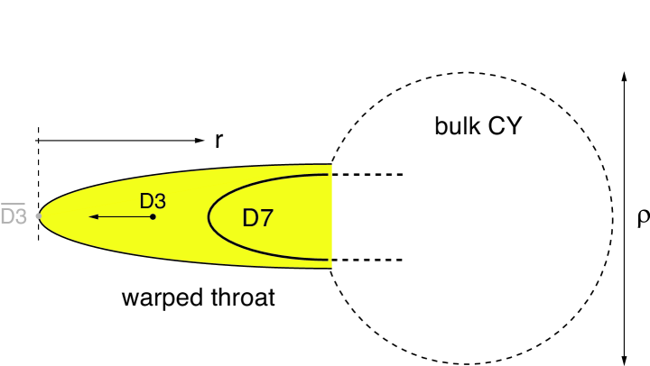
Figure 1: Cartoon of an embedded stack of D7-branes wrapping a four-cycle $\Sigma_{4}$, and a mobile D3-brane, in a warped throat region of a compact Calabi-Yau. In the scenario of [9] the D3-brane feels a force from an anti-D3-brane at the tip of the throat. Alternatively, in [14] it was argued that a D3-brane in the resolved warped deformed conifold background feels a force even in the absence of an anti-D3-brane. In this paper we consider an additional contribution to the D3-brane potential, coming from nonperturbative effects on D7-branes.

Let $\rho$ be the volume of a given four-cycle that admits a nonperturbative effect. The resulting superpotential is expected to be of the form [7]

$$W_{{\rm{np}}}(\rho)=A(\chi,X)e^{-a\rho}\,.$$ (1)

Here $a$ is a numerical constant and $A(\chi,X)$ is a holomorphic function of the complex structure moduli $\chi\equiv\{\chi_{1},\ldots,\chi_{h^{2,1}}\}$ and of the positions $X$ of any D3-branes in the internal space. The functional form of $A$ will depend on the particular four-cycle in question.

The prefactor $A(\chi,X)$ arises from a one-loop correction to the nonperturbative superpotential. For a Euclidean D3-brane superpotential, $A(\chi,X)$ represents a one-loop determinant of fluctuations around the instanton. In the case of D7-brane gauge dynamics the prefactor comes from a threshold correction to the gauge coupling on the D7-branes.

In the original KKLT proposal, the complex structure moduli acquired moderately large masses from the fluxes, and no probe D3-brane was present. Thus, it was possible to ignore the moduli-dependence of $A(\chi,X)$ and treat $A$ as a constant, albeit an unknown one. In the case of present interest (as in [9]), the complex structure moduli are still massive enough to be negligible, but there is at least one mobile D3-brane in the compact space, so we must write $A=A(X)$. (See [19] for a very general argument that no prefactor $A$ can be independent of a D3-brane location $X$.)

The goal of this paper is to compute $A(X)$. As we explained in the introduction, this has already been achieved in certain toroidal orientifolds [20], and the relevance of $A(X)$ for brane inflation has also been recognized [9, 20, 30]. Here we will use a closed-string channel method for computing $A(X)$, allowing us to study more general compactifications. In particular, we will give the first concrete results for $A(X)$ in the warped throats relevant for many brane inflation models.

2.2 D3-brane Potential After Volume Stabilization

The $F$-term part of the supergravity potential is

$$V_{F}=e^{\kappa_{4}^{2}{\cal K}}\left[{\cal K}^{i\bar{j}}D_{i}W\overline{D_{j}W}-3\kappa_{4}^{2}|W|^{2}\right]\,.$$ (2)

DeWolfe and Giddings [31] showed that the Kähler potential ${\cal K}$ in the presence of mobile D3-branes is

$$\kappa_{4}^{2}{\cal K}=-3\log\left[\rho+\bar{\rho}-\gamma k(X,\bar{X})\right]\equiv-2\log{\cal V}\,,$$ (3)

where $k(X,\bar{X})$ is the Kähler potential for the Calabi-Yau metric, i.e. the Kähler potential on the putative moduli space of a D3-brane probe, ${\cal V}$ is the physical volume of the internal space, and $\gamma$ is a constant. We address this volume-inflaton mixing in more detail in §6.1. For clarity we have assumed here that there is only one Kähler modulus, but our later analysis is more general.

The superpotential $W$ is the sum of a constant flux term [29] $W_{\rm flux}(\chi_{\star})=\int G\wedge\Omega\equiv W_{0}$ at fixed complex structure $\chi_{\star}$ and a term $W_{\rm np}$ (1) from nonperturbative effects,

$$W=W_{0}+A(X)e^{-a\rho}\,.$$ (4)

Equations (2) to (4) imply three distinct sources for corrections to the potential for D3-brane motion:

1. $m_{\cal K}$: The $X$-dependence of the Kähler potential ${\cal{K}}$ leads to a mass term familiar from the supergravity eta problem.

2. $m_{D}$: Sources of $D$-term energy, if present, will scale with the physical volume ${\cal V}$ and hence depend on the D3-brane location. This leads to a mass term for D3-brane displacements.

3. $m_{A}$: The prefactor $A(X)$ in the superpotential (4) leads to a mass term via the $F$-term potential $(\ref{equ:Fterm})$.

The masses $m_{\cal K}$ and $m_{D}$ were calculated explicitly in [9] and shown to be of order the Hubble parameter $H$. On the other hand, $m_{A}$ has been computed only for the toroidal orientifolds of [20]. It has been suggested [9] that there might exist non-generic configurations in which $m_{A}$ cancels against the other two terms. It is in these fine-tuned situations that D3-brane motion could produce slow-roll inflation. By computing $m_{A}$ explicitly, one can determine whether or not this hope is realized [18].

3 Warped Volumes and the Superpotential

3.1 The Role of the Warped Volume

The nonperturbative effects discussed in §2.1 depend exponentially on the warped volume of the associated four-cycle: the warped volume governs the instanton action in the case of Euclidean D3-branes, and the gauge coupling in the case of strong gauge dynamics on D7-branes. To see this, consider a warped background with the line element

$${\rm d}s^{2}=G_{\mu\nu}{\rm d}x^{\mu}{\rm d}x^{\nu}+G_{ij}{\rm d}Y^{i}{\rm d}Y^{j}\equiv h^{-{1/2}}(Y)g_{\mu\nu}{\rm d}x^{\mu}{\rm d}x^{\nu}+h^{{1/2}}(Y)g_{ij}{\rm d}Y^{i}{\rm d}Y^{j}\,,$$ (5)

where $Y^{i}$ and $g_{ij}$ are the coordinates and the unwarped metric on the internal space, respectively, and $h(Y)$ is the warp factor.

The Yang-Mills coupling $g_{7}$ of the $7+1$ dimensional gauge theory living on a stack of D7-branes is given by

$$g_{7}^{2}\equiv 2(2\pi)^{5}g_{s}(\alpha^{\prime})^{2}\,.$$ (6)

The action for gauge fields on D7-branes that wrap a four-cycle $\Sigma_{4}$ is

$$S=\frac{1}{2g_{7}^{2}}\int_{\Sigma_{4}}{\rm d}^{4}\xi\sqrt{g^{ind}}\,h(Y)\cdot\int{\rm d}^{4}x\sqrt{g}\ g^{\mu\alpha}g^{\nu\beta}\,{\rm Tr}\,F_{\mu\nu}F_{\alpha\beta}\,,$$ (7)

where $\xi_{i}$ are coordinates on $\Sigma_{4}$ and $g^{ind}$ is the metric induced on $\Sigma_{4}$ from $g_{ij}$. A key point is the appearance of a single power of $h(Y)$ [24]. Defining the warped volume of $\Sigma_{4}$,

$$V_{\Sigma_{4}}^{w}\equiv\int_{\Sigma_{4}}{\rm d}^{4}\xi\sqrt{g^{ind}}\,h(Y)\,$$ (8)

and recalling the D3-brane tension

$$T_{3}\equiv\frac{1}{(2\pi)^{3}g_{s}(\alpha^{\prime})^{2}}$$ (9)

we read off the gauge coupling of the four-dimensional theory from (7):

$$\frac{1}{g^{2}}=\frac{V_{\Sigma_{4}}^{w}}{g_{7}^{2}}=\frac{T_{3}V_{\Sigma_{4}}^{w}}{8\pi^{2}}\,.$$ (10)

In ${\cal{N}}=1$ super-Yang-Mills theory, the Wilsonian gauge coupling is the real part of a holomorphic function which receives one-loop corrections, but no higher perturbative corrections [33, 34, 35]. The modulus of the gaugino condensate superpotential in $SU(N_{D7})$ super-Yang-Mills with ultraviolet cutoff $M_{\rm{UV}}$ is given by

$$|W_{\rm np}|={16\pi^{2}}M_{\rm{UV}}^{3}\exp\Bigl{(}-\frac{1}{N_{D7}}\frac{8\pi^{2}}{g^{2}}\Bigr{)}\propto\exp\Bigl{(}-\frac{T_{3}V_{\Sigma_{4}}^{w}}{N_{D7}}\Bigr{)}\,.$$ (11)

The mobile D3-brane adds a flavor to the $SU(N_{D7})$ gauge theory, whose mass $m$ is a holomorphic function of the D3-brane coordinates. In particular, the mass vanishes when the D3-brane coincides with the D7-brane. In such a gauge theory, the superpotential is proportional to $m^{1/N_{D7}}$ [36]. Our explicit closed-string channel calculations will confirm this form of the superpotential.

In the case that the nonperturbative effect comes from a Euclidean D3-brane, the instanton action is

$$S=T_{3}\int_{\Sigma_{4}}{\rm d}^{4}\xi\sqrt{G^{ind}}=T_{3}\int_{\Sigma_{4}}{\rm d}^{4}\xi\sqrt{g^{ind}}\,h(Y)\equiv T_{3}V_{\Sigma_{4}}^{w}\,,$$ (12)

so that, just as in (7), the action depends on a single power of $h(Y)$. The modulus of the nonperturbative superpotential is then

$$|W_{\rm np}|\propto\exp\Bigl{(}-T_{3}V_{\Sigma_{4}}^{w}\Bigr{)}\,.$$ (13)

3.2 Corrections to the Warped Volumes of Four-Cycles

The displacement of a D3-brane in the compactification creates a slight distortion $\delta h$ of the warped background, and hence affects the warped volumes of four-cycles. The correction takes the form

$$\delta V_{\Sigma_{4}}^{w}\equiv\int_{\Sigma_{4}}{\rm d}^{4}Y\sqrt{g^{ind}(X;Y)}\,\delta h(X;Y)\,.$$ (14)

By computing this change in volume we will extract the dependence of the superpotential on the D3-brane location $X$. In the non-compact throat approximation, we will calculate $\delta V_{\Sigma_{4}}^{w}$ explicitly, and find that it is the real part of a holomorphic function $\zeta(X)$. Its imaginary part is determined by the integral of the Ramond-Ramond four-form perturbation $\delta C_{4}$ over $\Sigma_{4}$ (we will not compute this explicitly, but will be able to deduce the result using the holomorphy of $\zeta(X)$).

The nonperturbative superpotential of the form (1), generated by the gaugino condensation, is then determined by

$$A(X)=A_{0}\exp\Bigl{(}-\frac{T_{3}~{}\zeta(X)}{N_{D7}}\Bigr{)}\,.$$ (15)

We have introduced an unimportant constant $A_{0}$ that depends on the values at which the complex structure moduli are stabilized, but is independent of the D3-brane position. As remarked above, computing (15) is equivalent to computing the dependence of the threshold correction to the gauge coupling on the mass $m$ of the flavor coming from strings that stretch from the D7-branes to the D3-brane.

In the case of Euclidean D3-branes, the change in the instanton action is proportional to the change in the warped four-cycle volume. Hence, the nonperturbative superpotential is of the form (1) with

$$A(X)=A_{0}\exp\Bigl{(}-T_{3}~{}\zeta(X)\Bigr{)}\,.$$ (16)

In this case, computing (14) is equivalent to computing the D3-brane dependence of an instanton fluctuation determinant.

Finally, we can write a unified expression that applies to both sources of nonperturbative effects:

$$A(X)=A_{0}\exp\Bigl{(}-\frac{T_{3}~{}\zeta(X)}{n}\Bigr{)}\,,$$ (17)

where $n=N_{D7}$ for the case of gaugino condensation on D7-branes and $n=1$ for the case of Euclidean D3-branes.

4 D3-brane Backreaction

4.1 The Green’s Function Method

A D3-brane located at some position $X$ in a six-dimensional space with coordinates $Y$ acts as a point source for a perturbation $\delta h$ of the geometry:

$$-\nabla_{Y}^{2}\delta h(X;Y)={\cal C}\,\left[\frac{\delta^{(6)}(X-Y)}{\sqrt{g(Y)}}-\rho_{bg}(Y)\right]\,.$$ (18)

That is, the perturbation $\delta h$ is a Green’s function for the Laplace problem on the background of interest. Here ${\cal C}\equiv 2\kappa_{10}^{2}T_{3}=(2\pi)^{4}g_{s}(\alpha^{\prime})^{2}$ ensures the correct normalization of a single D3-brane source term relative to the four-dimensional Einstein-Hilbert action. A consistent flux compactification contains a background charge density $\rho_{bg}(Y)$ which satisfies

$$\int{\rm d}^{6}Y\sqrt{g}\,\rho_{bg}(Y)=1\,$$ (19)

to account for the Gauss’s law constraint on the compact space [6].

To solve (18), we first solve

$$-\nabla_{Y^{\prime}}^{2}\Phi(Y;Y^{\prime})=-\nabla_{Y}^{2}\Phi(Y;Y^{\prime})=\frac{\delta^{(6)}(Y-Y^{\prime})}{\sqrt{g}}-\frac{1}{V_{6}}\,,$$ (20)

where $V_{6}\equiv\int{\rm d}^{6}Y\sqrt{g}$. The solution to (18) is then

$$\delta h(X;Y)={\cal C}\,\Bigl{[}\Phi(X;Y)-\int{\rm d}^{6}Y^{\prime}\sqrt{g}\,\Phi(Y;Y^{\prime})\rho_{bg}(Y^{\prime})\Bigr{]}\,.$$ (21)

We note for later use that

$$-\nabla_{X}^{2}\delta h(X;Y)={\cal C}\,\left[{\delta^{(6)}(X-Y)\over\sqrt{g(X)}}-\frac{1}{V_{6}}\right]\,.$$ (22)

This relation is independent of the form of the background charge $\rho_{bg}$.

To compute $A(X)$ from (17), we simply solve for the Green’s function $\delta h$ obeying (18) and then integrate $\delta h$ over the four-cycle of interest, according to (14).

4.2 Comparison with the Open-String Approach

Let us show that this supergravity (closed-string channel) method is consistent with the results of BHK [20], where the correction to the gaugino condensate superpotential was derived via a one-loop open-string computation.

The analysis of [20] applied to configurations of D7-branes and D3-branes on certain toroidal orientifolds, e.g. $T^{2}\times T^{4}/\mathbb{Z}_{2}$. We introduce a complex coordinate $X$ for the position of the D3-branes on $T^{2}$, as well as a complex structure modulus $\tau$ for $T^{2}$, and without loss of generality we set the volume of $T^{4}/\mathbb{Z}_{2}$ to unity. Let us consider the case where all the D7-branes wrap $T^{4}/\mathbb{Z}_{2}$ and sit at the origin $X=0$ in $T^{2}$.

The goal is to determine the dependence of the gauge coupling on the position $X$ of a D3-brane. (The location of the D3-brane in the $T^{4}/\mathbb{Z}_{2}$ wrapped by the D7-branes is immaterial.) For this purpose, we may omit terms computed in [20] that depend only on the complex structure and not on the D3-brane location. Such terms will only affect the D3-brane potential by an overall constant.

Then, the relevant terms from equation (44) of [20], in our notation, are

$$\delta\Bigl{(}\frac{8\pi^{2}}{g^{2}}\Bigr{)}=\frac{1}{4\pi\,{\rm Im}(\tau)}\Bigl{[}{\rm{Im}}(X)\Bigr{]}^{2}-\frac{1}{2}{\rm{ln}}\left|\vartheta_{1}\left(\frac{X}{2\pi}\Bigl{|}\Bigr{.}\tau\right)\right|^{2}\,.$$ (23)

Let us now compare (23) to the result of the supergravity computation. In principle, the prescription of equation (14) is to integrate the Green’s function on a six-torus over the wrapped four-torus. However, we notice that this procedure of integration will reduce the six-dimensional Laplace problem to the Laplace problem on the two-torus parametrized by $X$,

$$-\nabla_{X}^{2}\delta h(X;0)={\cal C}\,\left[\delta^{(2)}(X)-\frac{1}{V_{T^{2}}}\right]\,,$$ (24)

where $V_{T^{2}}=8\pi^{2}\,{\rm Im}(\tau)$. The correction to the gauge coupling, in the supergravity approach, is then proportional to $\delta h(X;0)$. Solving (24) and using (10), we get exactly (23). We conclude that our method precisely reproduces the results of [20], at least for those terms that directly enter the D3-brane potential.

4.3 A Model for the Four-Cycles

The closed-string channel approach to calculating $A(X)$ is well-defined for any given background, but further assumptions are required when no complete metric for the compactification is available. Fortunately, explicit metrics are available for many non-compact Calabi-Yau spaces, and at the same time, the associated warped throat regions are of particular interest for inflationary phenomenology. For a given warped throat geometry, our approach is to compute the D3-brane backreaction on specific four-cycles in the non-compact, asymptotically conical space. We will demonstrate that this gives an excellent approximation to the backreaction in a compactification in which the same warped throat is glued into a compact bulk. In particular, we will show in §6.2 that the physical effect in question is localized in the throat, i.e. is determined primarily by the shape of the four-cycle in the highly warped region. The model therefore only depends on well-known data, such as the specific warped metric and the embedding equations of the four-cycles, and is insensitive to the unknown details of the unwarped bulk. In principle, our method can be extended to general compact models for which metric data is available.

It still remains to identify the four-cycles responsible for nonperturbative effects in this model of a warped throat attached to a compact space. Such a space will in general have many Kähler moduli, and hence, assuming that stabilization is possible at all, will have many contributions to the nonperturbative superpotential. The most relevant term, for the purpose of determining the D3-brane potential, is the term corresponding to the four-cycle closest to the D3-brane. For a D3-brane moving in the throat region, this is the four-cycle that reaches farthest down the throat. In addition, the gauge theory living on the corresponding D7-branes should be making an important contribution to the superpotential.

The nonperturbative effects of interest are present only when the four-cycle satisfies an appropriate topological condition [23], which we will not discuss in detail. This topological condition is, of course, related to the global properties of the four-cycle, whereas the effect we compute is dominated by the part of the four-cycle in the highly-warped throat region, and is insensitive to details of the four-cycle in the unwarped region. That is, our methods are not sensitive to the distinction between four-cycles that do admit nonperturbative effects, and those that do not. We therefore propose to model the four-cycles producing nonperturbative effects with four-cycles that are merely supersymmetric, i.e. can be wrapped supersymmetrically by D7-branes. Many members of the latter class are not members of the former, but as the shape of the cycle in the highly-warped region is the only important quantity, we expect this distinction to be unimportant.

We are therefore led to consider the backreaction of a D3-brane on the volume of a stack of supersymmetric D7-branes wrapping a four-cycle in a warped throat geometry. The simplest configuration of this sort is a supersymmetric ‘flavor brane’ embedding of several D7-branes in a conifold [39, 40, 41].

5 Backreaction in Warped Conifold Geometries

We now recall some relevant geometry. The singular conifold is a non-compact Calabi-Yau threefold defined as the locus

$$\sum_{i=1}^{4}z_{i}^{2}=0$$ (25)

in $\mathbb{C}^{4}$. After a linear change of variables ($w_{1}=z_{1}+iz_{2},w_{2}=z_{1}-iz_{2}$, etc.), the constraint (25) becomes

$$w_{1}w_{2}-w_{3}w_{4}=0\,.$$ (26)

The Calabi-Yau metric on the conifold is

$${\rm d}s_{6}^{2}={\rm d}r^{2}+r^{2}{\rm d}s_{T^{1,1}}^{2}\,.$$ (27)

The base of the cone is the $T^{1,1}$ coset space $(SU(2)_{A}\times SU(2)_{B})/U(1)_{R}$ whose metric in angular coordinates $\theta_{i}\in[0,\pi],\phi_{i}\in[0,2\pi],\psi\in[0,4\pi]$ is

$${\rm d}s_{T^{1,1}}^{2}=\frac{1}{9}\Bigl{(}{\rm d}\psi+\sum_{i=1}^{2}\cos\theta_{i}\,{\rm d}\phi_{i}\Bigr{)}^{2}+\frac{1}{6}\sum_{i=1}^{2}\Bigl{(}{\rm d}\theta_{i}^{2}+\sin^{2}\theta_{i}\,{\rm d}\phi_{i}^{2}\Bigr{)}\,.$$ (28)

A stack of $N$ D3-branes placed at the singularity $w_{i}=0$ backreacts on the geometry, producing the ten-dimensional metric

$${\rm d}s_{10}^{2}=h^{-1/2}(r){\rm d}x_{4}^{2}+h^{1/2}(r){\rm d}s_{6}^{2}\ ,$$ (29)

where the warp factor is

$$h(r)=\frac{27\pi g_{s}N(\alpha^{\prime})^{2}}{4r^{4}}\ .$$ (30)

This is the $AdS_{5}\times T^{1,1}$ background of type IIB string theory, whose dual ${\cal N}=1$ supersymmetric conformal gauge theory was constructed in [42]. The dual is an $SU(N)\times SU(N)$ gauge theory coupled to bi-fundamental chiral superfields $A_{1},A_{2},B_{1},B_{2}$, each having $R$-charge $1/2$. Under the $SU(2)_{A}\times SU(2)_{B}$ global symmetry, the superfields transform as doublets. If we further add $M$ D5-branes wrapped over the two-cycle inside $T^{1,1}$, then the gauge group changes to $SU(N+M)\times SU(N)$, giving a cascading gauge theory [15, 12]. The metric remains of the form (29), but the warp factor is modified to [15, 43]

$$h(r)=\frac{27\pi(\alpha^{\prime})^{2}}{4r^{4}}\Bigl{[}g_{s}N+b(g_{s}M)^{2}\log\Bigl{(}\frac{r}{r_{0}}\Bigr{)}+\frac{1}{4}b(g_{s}M)^{2}\Bigr{]}\,,$$ (31)

with $b\equiv\frac{3}{2\pi}$, and $r_{0}\sim\varepsilon^{2/3}e^{2\pi N/(3g_{s}M)}$. If an extra D3-brane is added at small $r$, it produces a small change of the warp factor, $\delta h=\frac{27\pi g_{s}(\alpha^{\prime})^{2}}{4r^{4}}+{\cal O}(r^{-11/2})$. A precise determination of $\delta h$ on the conifold, using the Green’s function method, is one of our goals in this paper. As discussed above, this needs to be integrated over a supersymmetric four-cycle.

5.1 Supersymmetric Four-Cycles in the Conifold

The complex coordinates $w_{i}$ can be related to the real coordinates $(r,\theta_{i},\phi_{i},\psi)$ via

$$w_{1} = r^{3/2}e^{\frac{i}{2}(\psi-\phi_{1}-\phi_{2})}\sin\frac{\theta_{1}}{2}\sin\frac{\theta_{2}}{2}\,,$$ (32)

$$w_{2} = r^{3/2}e^{\frac{i}{2}(\psi+\phi_{1}+\phi_{2})}\cos\frac{\theta_{1}}{2}\cos\frac{\theta_{2}}{2}\,,$$ (33)

$$w_{3} = r^{3/2}e^{\frac{i}{2}(\psi+\phi_{1}-\phi_{2})}\cos\frac{\theta_{1}}{2}\sin\frac{\theta_{2}}{2}\,,$$ (34)

$$w_{4} = r^{3/2}e^{\frac{i}{2}(\psi-\phi_{1}+\phi_{2})}\sin\frac{\theta_{1}}{2}\cos\frac{\theta_{2}}{2}\,.$$ (35)

It was shown in [41] that the following holomorphic four-cycles admit supersymmetric D7-branes:

$$f(w_{i})\equiv\prod_{i=1}^{4}w_{i}^{p_{i}}-\mu^{P}=0\,.$$ (36)

Here $p_{i}\in\mathbb{Z}$, $P\equiv\sum_{i=1}^{4}p_{i}$, and $\mu\in\mathbb{C}$ are constants defining the embedding of the D7-branes. In real coordinates the embedding condition (36) becomes

$$\psi(\phi_{1},\phi_{2}) = n_{1}\phi_{1}+n_{2}\phi_{2}+\psi_{s}\,,$$ (37)

$$r(\theta_{1},\theta_{2}) = r_{\rm min}\left[x^{1+n_{1}}(1-x)^{1-n_{1}}y^{1+n_{2}}(1-y)^{1-n_{2}}\right]^{-1/6}\,,$$ (38)

where

$$r_{\rm min}^{3/2} \equiv |\mu|\,,$$ (39)

$$\frac{1}{2}\psi_{s} \equiv {\rm arg}(\mu)+\frac{2\pi s}{P}\,,\quad s\in\{0,1,\dots,P-1\}\,.$$ (40)

We have defined the coordinates

$$x\equiv\sin^{2}\frac{\theta_{1}}{2}\,,\quad y\equiv\sin^{2}\frac{\theta_{2}}{2}$$ (41)

and the rational winding numbers

$$n_{1}\equiv\frac{p_{1}-p_{2}-p_{3}+p_{4}}{P}\,,\quad n_{2}\equiv\frac{p_{1}-p_{2}+p_{3}-p_{4}}{P}\,.$$ (42)

To compute the integral over the four-cycle we will need the volume form on the wrapped D7-brane, which is

$${\rm d}\theta_{1}{\rm d}\theta_{2}{\rm d}\phi_{1}{\rm d}\phi_{2}\,\sqrt{g^{ind}}=\frac{V_{T^{1,1}}}{16\pi^{3}}\,r^{4}\,{\cal G}(x,y)\,{\rm d}x{\rm d}y{\rm d}\phi_{1}{\rm d}\phi_{2}\,,$$ (43)

where

$${\cal G}(x,y) \equiv \frac{(1+n_{1})^{2}}{2}\frac{1}{x(1-x)}-2n_{1}\frac{1}{1-x}$$ (44)

$$+ \frac{(1+n_{2})^{2}}{2}\frac{1}{y(1-y)}-2n_{2}\frac{1}{1-y}-1\,.$$

In (43) we defined the volume of $T^{1,1}$

$$V_{T^{1,1}}\equiv\int{\rm d}^{5}\Psi\sqrt{g_{T^{1,1}}}=\frac{16\pi^{3}}{27}\,,$$ (45)

with $\Psi$ standing for all five angular coordinates on $T^{1,1}$.

For applications to brane inflation, we are interested in four-cycles that do not reach the tip of the conifold ($|n_{i}|\leq 1$). Two simple special cases of (36) have this property:

• Ouyang embedding [40]:

  $$w_{1}=\mu\,.$$

• Karch-Katz embedding [39]:

  $$w_{1}w_{2}=\mu^{2}\,.$$

Analogous supersymmetric four-cycles are known [45] in some more complicated asymptotically conical spaces, such as cones over $Y^{p,q}$ manifolds. We will consider this case in §5.4 and in Appendix C.

5.2 Relation to the Dual Gauge Theory Computation

The calculation of $\delta h$ and its integration over a holomorphic four-cycle is not sensitive to the background warp factor. Let us discuss a gauge theory interpretation of the calculation when we choose the background warp factor from (30), i.e. we ignore the effect of $M$ wrapped D5-branes. Here the gauge theory is exactly conformal, and we may invoke the AdS/CFT correspondence to give a simple meaning to the multipole expansion of $\delta h$,

$$\delta h=\frac{27\pi g_{s}(\alpha^{\prime})^{2}}{4r^{4}}\left[1+\sum_{i}\frac{c_{i}f_{i}(\theta_{1},\theta_{2},\phi_{1},\phi_{2},\psi)}{r^{\Delta_{i}}}\right]\ .$$ (46)

In the dual gauge theory, the $c_{i}$ are proportional to the expectation values of gauge-invariant operators ${\cal O}_{i}$ determined by the position of the D3-brane [25]. Among these operators a special role is played by the chiral operators of $R$-charge $k$, ${\rm Tr}[A_{\alpha_{1}}B_{\dot{\beta}_{1}}A_{\alpha_{2}}B_{\dot{\beta}_{2}}\ldots A_{\alpha_{k}}B_{\dot{\beta}_{k}}]$, symmetric in both the dotted and the undotted indices. These operators have exact dimensions $\Delta_{i}^{\rm chiral}=3k/2$ and transform as $(k/2,k/2)$ under the $SU(2)_{A}\times SU(2)_{B}$ symmetry. In addition to these operators, many non-chiral operators, whose dimensions $\Delta_{i}$ are not quantized [46], acquire expectation values and therefore affect the multipole expansion of the warp factor. But remarkably, all these non-chiral contributions vanish upon integration over a holomorphic four-cycle. Therefore, the contributing terms in $\delta h$ have the simple form [25]

$$\delta h_{\rm chiral}=\frac{27\pi g_{s}(\alpha^{\prime})^{2}}{4r^{4}}\left[1+\sum_{k=1}^{\infty}\frac{\left(f_{a_{1}\dots a_{k}}\widehat{z}_{a_{1}\dots a_{k}}+c.c.\right)}{r^{3k/2}}\right]\ ,$$ (47)

where $f_{a_{1}\dots a_{k}}\sim\bar{\epsilon}_{a_{1}}\bar{\epsilon}_{a_{2}}\ldots\bar{\epsilon}_{a_{k}}$ for a D3-brane positioned at $z_{a}=\epsilon_{a}$. Above, $\widehat{z}_{a_{1}\dots a_{k}}$ are the normalized spherical harmonics on $T^{1,1}$ that transform as $(k/2,k/2)$ under the $SU(2)_{A}\times SU(2)_{B}$. The normalization factors are defined in Appendix A.

The leading term in (46), which falls off as $1/r^{4}$, gives a logarithmic divergence at large $r$ when integrated over a four-cycle. We note that this term does not appear if we define $\delta h$ as the solution of (18) with $\sqrt{g}\,\rho_{bg}(Y)=\delta^{(6)}(Y-X_{0})$. This corresponds to evaluating the change in the warp factor, $\delta h$, created by moving the D3-brane to $X$ from some reference point $X_{0}$. If we choose the reference point $X_{0}$ to be at the tip of the cone, $r=0$, then (46) is modified to

$$\delta h=\frac{27\pi g_{s}(\alpha^{\prime})^{2}}{4r^{4}}\left[\sum_{i}\frac{c_{i}f_{i}(\theta_{1},\theta_{2},\phi_{1},\phi_{2},\psi)}{r^{\Delta_{i}}}\right]\ .$$ (48)

An advantage of this definition is that now there is a precise correspondence between our calculation and the expectation values of operators in the dual gauge theory.

5.3 Results for the Conifold

We are now ready to compute the D3-brane-dependent correction to the warped volume of a supersymmetric four-cycle in the conifold. Using the Green’s function on the singular conifold (80), which we derive in Appendix A, and the explicit form of the induced metric $\sqrt{g^{ind}}$ (43), we carry out integration term by term and find that most terms in (14) do not contribute. We relegate the details of this computation to Appendix B. As we demonstrate in Appendix B, the terms that do not cancel are precisely those corresponding to (anti)chiral deformations of the dual gauge theory.

Integrating (48) term by term as prescribed in (14), we find that the final result for a general embedding (36) is

$$T_{3}\,\delta V_{\Sigma_{4}}^{w}=T_{3}\,{\rm Re}\left(\zeta(w_{i})\right)=-{\rm Re}\left(\log\left[\frac{\mu^{P}-\prod_{i=1}^{4}w_{i}^{p_{i}}}{\mu^{P}}\right]\right)\,,$$ (49)

so that

$$A=A_{0}\left(\frac{\mu^{P}-\prod_{i=1}^{4}w_{i}^{p_{i}}}{\mu^{P}}\right)^{1/n}\,.$$ (50)

Comparing to (36), we see that $A$ is proportional to a power of the holomorphic equation that specifies the embedding. For $n=N_{D7}$ coincident D7-branes, this power is $1/n$. This behavior agrees with the results of [19]; note in particular that when $n=1$, (50) has a simple zero everywhere on the four-cycle, as required by [19].

Finally, let us specialize to the two cases of particular interest, the Ouyang [40] and Karch-Katz [39] embeddings in which the four-cycle does not reach all the way to the tip of the throat. For the Ouyang embedding we find

$$A(w_{1})=A_{0}\left(\frac{\mu-w_{1}}{\mu}\right)^{1/n}\,,$$ (51)

whereas for the Karch-Katz embedding we have

$$A(w_{1},w_{2})=A_{0}\left(\frac{\mu^{2}-w_{1}w_{2}}{\mu^{2}}\right)^{1/n}\,.$$ (52)

5.4 Results for $Y^{p,q}$ Cones

Recently, a new infinite class of Sasaki-Einstein manifolds $Y^{p,q}$ of topology $S^{2}\times S^{3}$ was discovered [47, 48]. The ${\cal N}=1$ superconformal gauge theories dual to $AdS_{5}\times Y^{p,q}$ were constructed in [49]. These quiver theories, which live on $N$ D3-branes at the apex of the Calabi-Yau cone over $Y^{p,q}$, have gauge groups $SU(N)^{2p}$, bifundamental matter, and marginal superpotentials involving both cubic and quartic terms. Addition of $M$ D5-branes wrapped over the $S^{2}$ at the apex produces a class of cascading gauge theories whose warped cone duals were constructed in [50]. A D3-brane moving in such a throat could also serve as a model of D-brane inflation [14].

Having described the calculation for the singular conifold in some detail, we now cite the results of an equivalent computation for cones over $Y^{p,q}$ manifolds. More details can be found in Appendix C.

Supersymmetric four-cycles in $Y^{p,q}$ cones are defined by the following embedding condition [45]

$$f(w_{i})\equiv\prod_{i=1}^{3}w_{i}^{p_{i}}-\mu^{2p_{3}}=0\,,$$ (53)

where the complex coordinates $w_{i}$ are defined in Appendix C. Integration of the Green’s function over the four-cycle leads to the following result for the perturbation to the warped volume

$$T_{3}\,\delta V_{\Sigma_{4}}^{w}=T_{3}\,{\rm Re}\left(\zeta(w_{i})\right)=-{\rm Re}\left(\log\left[\frac{\mu^{2p_{3}}-\prod_{i=1}^{3}w_{i}^{p_{i}}}{\mu^{2p_{3}}}\right]\right)\,,$$ (54)

so that

$$A=A_{0}\left(\frac{\mu^{2p_{3}}-\prod_{i=1}^{3}w_{i}^{p_{i}}}{\mu^{2p_{3}}}\right)^{1/n}\,.$$ (55)

5.5 General Compactifications

The arguments in [19], which were based on studying the change in the theta angle as one moves the D3-brane around the D7-branes, indicate that the correction is a section of a bundle called the ‘divisor bundle’. This section has a zero at the location of the D7-branes. The correction has to live in a non-trivial bundle since a holomorphic function on a compact space would be a constant. In the non-compact examples we considered above we can work in only one coordinate patch and obtain the correction as a simple function, the function characterizing the embedding. Strictly speaking, the arguments in [19] were made for the case that the superpotential is generated by wrapped D3-instantons. But the same arguments can be used to compute the correction for the gauge coupling on D7-branes.

In summary, we have explicitly computed the modulus of $A$, and found a result in perfect agreement with the analysis of the phase of $A$ in [19]. One has a general answer of the form

$$A(w_{i})=A_{0}~{}\Bigl{(}f(w_{i})\Bigr{)}^{1/n}\,,$$ (56)

where $f$ is a section of the divisor bundle and $f(w_{i})=0$ specifies the location of the D7-branes.

6 Compactification Effects

6.1 Holomorphy of the Gauge Coupling

In compactifications with mobile D3-branes, the identification of holomorphic Kähler moduli and holomorphic gauge couplings is quite subtle. This has become known as the ‘rho problem’ [20, 24]. Let us recall the difficulty. In the internal metric $g_{ij}$ appearing in (5), we can identify the breathing mode of the compact space via

$$g_{ij}\equiv\tilde{g}_{ij}e^{2u}\,,$$ (57)

where $\tilde{g}_{ij}$ is a fiducial metric. In the following, all quantities computed from $\tilde{g}_{ij}$ will be denoted by a tilde. The Born-Infeld kinetic term for a D3-brane, expressed in Einstein frame and in terms of complex coordinates $X,\bar{X}$ on the brane configuration space, is then

$$S_{kin}=-T_{3}\int{\rm d}^{4}x\sqrt{g}e^{-4u}\partial_{\mu}X^{i}\partial^{\mu}\bar{X}^{\bar{j}}\tilde{g}_{i\bar{j}}\,.$$ (58)

DeWolfe and Giddings argued in [31] that to reproduce this volume scaling, as well as the known no-scale, sequestered property of the D3-brane action in this background, the Kähler potential must take the form

$${\kappa_{4}^{2}}{\cal K}=-3\log{e^{4u}}\,,$$ (59)

with the crucial additional requirement that

$$\partial_{i}\partial_{\bar{j}}e^{4u}\propto\tilde{g}_{i\bar{j}}\,,$$ (60)

so that $e^{4u}$ contains a term proportional to the Kähler potential $k(X,\bar{X})$ for the fiducial Calabi-Yau metric. Comparing (58) to the kinetic term derived from (59), we find in fact

$$\partial_{i}\partial_{\bar{j}}e^{4u}=-\left(\frac{\kappa_{4}^{2}T_{3}}{3}\right)k_{,i\bar{j}}\,.$$ (61)

We can now define the holomorphic volume modulus $\rho$ as follows. The real part of $\rho$ is given by

$$\rho+\bar{\rho}\equiv e^{4u}+\left(\frac{\kappa_{4}^{2}T_{3}}{3}\right)k(X,\bar{X})$$ (62)

and the imaginary part is the axion from the Ramond-Ramond four-form potential. As explained in [9], this is consistent with the fact that the axion moduli space is a circle that is non-trivially fibered over the D3-brane moduli space.

Next, the gauge coupling on a D7-brane is easily seen to be proportional to the breathing mode of the metric, $e^{4u}\equiv\rho+\bar{\rho}-\left(\frac{1}{3}{\kappa_{4}^{2}}T_{3}\right)k(X,\bar{X})$, which is not the real part of holomorphic function on the brane moduli space. However, supersymmetry requires that the gauge kinetic function is a holomorphic function of the moduli. This conflict is the rho problem.

We can trace this problem to an incomplete inclusion of the backreaction due to the D3-brane. Through (62), the physical volume modulus $e^{4u}$ has been allowed to depend on the D3-brane position. That is, the difference between the holomorphic modulus $\rho$ and the physical modulus $e^{4u}$ is affected by the D3-brane position. This was necessary in order to recover the known properties of the brane/volume moduli space. Notice from (62) that the strength of this open-closed mixing is controlled by ${\kappa_{4}^{2}}T_{3}$, and so is manifestly a consequence of D3-brane backreaction in the compact space. However, as we explained in §3, the warp factor $h$ also depends on the D3-brane position, again via backreaction. To include the effects of the brane on the breathing mode, but not on the warp factor, is not consistent. One might expect that consideration of the correction $\delta h$ to the warp factor would restore holomorphy and resolve the rho problem. We will now see that this is indeed the case.

What we find is that the uncorrected warped volume $(V_{\Sigma_{4}}^{w})_{0}$, as well as the correction $\delta V_{\Sigma_{4}}^{w}$, are both non-holomorphic, but their non-holomorphic pieces precisely cancel, so that the corrected warped volume $V_{\Sigma_{4}}^{w}$ is the real part of a holomorphic function of the moduli $\rho$ and $X$.

First, we separate the constant, zero-mode, piece of the warp factor:

$$h(X;Y)=h_{0}+\delta h(X;Y)\,.$$ (63)

By definition $\delta h(X;Y)$ integrates to zero over the compact manifold,

$$\int{\rm d}^{6}Y\sqrt{g(Y)}\,\delta h(X;Y)=0\,.$$ (64)

This implies that the factor of the volume that appears in the four-dimensional Newton constant is unaffected by $\delta h$. Thus we have $\kappa_{4}^{-2}=\kappa_{10}^{-2}h_{0}\tilde{V}_{6}$. We define the uncorrected warped volume via

$$(V_{\Sigma_{4}}^{w})_{0}\equiv\int_{\Sigma_{4}}{\rm d}^{4}\xi\sqrt{g^{ind}}\,h_{0}=e^{4u(X,\bar{X})}\,h_{0}\,\tilde{V}_{\Sigma_{4}}\,.$$ (65)

This is non-holomorphic because of the prefactor $e^{4u(X,\bar{X})}$. In particular, using (62), we have

$$(V_{\Sigma_{4}}^{w})_{0}=-\left(\frac{\kappa_{4}^{2}T_{3}}{3}\right)\tilde{V}_{\Sigma_{4}}\,h_{0}\,k(X,\bar{X})+[{\rm hol.}+{\rm antihol.}]\,.$$ (66)

We next consider $\delta h$. When the D3-brane is not coincident with the four-cycle of interest, we find from (22) that $\delta h$ obeys

$$\nabla_{X}^{2}\delta h(X;Y)=\frac{\cal{C}}{V_{6}}\,$$ (67)

where ${\cal C}\equiv 2\kappa_{10}^{2}T_{3}=2\kappa_{4}^{2}T_{3}h_{0}\tilde{V}_{6}$. Hence, $\delta h$ is not the real part of a holomorphic function of $X$. The source of the deviation from holomorphy is the term $\frac{1}{V_{6}}$ in (22). Although this term is superficially similar to a constant background charge density, it is independent of the density $\rho_{bg}(Y)$ of physical D3-brane charge in the internal space, which has coordinates $Y$. Instead, $\frac{1}{V_{6}}$ may be thought of as a ‘background charge’ on the D3-brane moduli space, which has coordinates $X$. From this perspective, it is the Gauss’s law constraint on the D3-brane moduli space that forces $\delta h$ to be non-holomorphic.

In complex coordinates, using the metric $\tilde{g}$, and noting that $\tilde{V}_{6}=V_{6}\,e^{-6u}$, (67) may be written as

$$\tilde{g}^{i\bar{j}}\partial_{i}\partial_{\bar{j}}\delta h=\kappa_{4}^{2}T_{3}\,h_{0}\,e^{-4u}\,,$$ (68)

where because the compact space is Kähler, we can write the Laplacian using partial derivatives. It follows that

$$\delta h=\left(\frac{\kappa_{4}^{2}T_{3}}{3}\right)h_{0}\,e^{-4u}k(X,\bar{X})+[{\rm hol.}+{\rm antihol.}]\,.$$ (69)

The omitted holomorphic and antiholomorphic terms are precisely those that we computed in the preceding sections. Furthermore, recalling the definition (14), we have

$$\delta V_{\Sigma_{4}}^{w}=\left(\frac{\kappa_{4}^{2}T_{3}}{3}\right)h_{0}\,\tilde{V}_{\Sigma_{4}}k(X,\bar{X})+[\zeta(X)+\overline{\zeta(X)}]\,.$$ (70)

The non-holomorphic first term in (70) precisely cancels the non-holomorphic term in $(V_{\Sigma_{4}}^{w})_{0}$ (66), so that

$$V_{\Sigma_{4}}^{w}=(V_{\Sigma_{4}}^{w})_{0}+\delta V_{\Sigma_{4}}^{w}=\tilde{V}_{\Sigma_{4}}\,h_{0}\,(\rho+\bar{\rho})+[\zeta(X)+\overline{\zeta(X)}]\,.$$ (71)

We conclude that $V_{\Sigma_{4}}^{w}$ can be the real part of a holomorphic function.

To summarize, we have seen that the background charge term in (22), which was required by a constraint analogous to Gauss’s law on the D3-brane moduli space, causes $\delta V_{\Sigma_{4}}^{w}$ to have a non-holomorphic term proportional to $k(X,\bar{X})$. Furthermore, the DeWolfe-Giddings Kähler potential produces a well-known non-holomorphic term, also proportional to $k(X,\bar{X})$, in the uncorrected warped volume $(V_{\Sigma_{4}}^{w})_{0}$. We found that these two terms precisely cancel, so that the total warped volume $V_{\Sigma_{4}}^{w}=(V_{\Sigma_{4}}^{w})_{0}+\delta V_{\Sigma_{4}}^{w}$ can be holomorphic. Thus, the corrected gauge coupling on D7-branes, and the corrected Euclidean D3-brane action, are holomorphic.

Note that, as a consequence of this discussion, the holomorphic part of the correction to the volume changes under Kähler transformations of $k(X,\bar{X})$. This implies that the correction is in a bundle whose field strength is proportional to the Kähler form.

6.2 Model-Dependent Effects from the Bulk

In §2.2, we listed three contributions to the potential for D3-brane motion. The first two were given explicitly in [9], and we have computed the third. It is now important to ask whether this is an exhaustive list: in other words, might there be further effects that generate D3-brane mass terms of order $H$? In particular, could coupling of the throat to a compact bulk generate corrections to our results, and hence adjust the brane potential?

First, let us justify our approach of using noncompact warped throats to model D3-brane potentials in compact spaces with finite warped throat regions. The idea is that the effect of the D3-brane on a four-cycle is localized in that portion of the four-cycle that is deepest in the throat. Comparing (43) to (48), we see that all corrections to the warped volume scale inversely with $r$, and are therefore supported in the infrared region of the throat. Hence, as anticipated in §4.3, the effects of interest are automatically concentrated in the well-understood region of high warping, far from the model-dependent region where the throat is glued into the rest of the compact space. This is true even though a typical four-cycle will have most of its volume in the bulk, outside the highly warped region. The perturbation due to the D3-brane already falls off faster than $r^{-4}$ in the throat, where the measure factor is $r^{4}$, and in the bulk the perturbation will diminish even more rapidly. Except in remarkable cases, the diminution of the perturbation will continue to dominate the growth of the measure factor. A similar argument reinforces our assertion that the dominant effect on a D3-brane comes from whichever wrapped brane descends farthest into the throat.

We conclude that the effects of the gluing region, where the throat meets the bulk, and of the bulk itself, produce negligible corrections to the terms we have computed. Fortunately, the leading effects are concentrated in the highly warped region, where one has access to explicit metrics and can do complete computations.

We have now given a complete account of the nonperturbative superpotential. However, the Kähler potential is not protected against perturbative corrections, which could conceivably contribute to the low-energy potential for D3-brane motion. Explicit results are not available for general compact spaces (see, however, [21, 22]); here we will simply argue that these corrections can be made negligible. Recall that the DeWolfe-Giddings Kähler potential provides a mixing between the volume and the D3-brane position that generates brane mass terms of order $H$. Any further corrections to the Kähler potential, whether from string loops or sigma-model loops, will be subleading in the large-volume, weak-coupling limit, and will therefore generically give mass terms that are small compared to $H$. In addition, the results of [52] give some constraints on $\alpha^{\prime}$ corrections to warped throat geometries. We leave a systematic study of this question for the future.

7 Implications and Conclusion

We have used a supergravity approach (see also [24]) to study the D3-brane corrections to the nonperturbative superpotential induced by D7-branes or Euclidean D3-branes wrapping four-cycles of a compactification. This has been a key, unknown element of the potential governing D3-brane motion in such a compactification. We integrated the perturbation to the background warping due to the D3-brane over the wrapped four-cycle. The resulting position-dependent correction to the warped four-cycle volume modifies the strength of the nonperturbative effect, which in turn implies a force on the D3-brane. This computation is the closed-string channel dual of the threshold correction computation of [20], and we showed that the closed-string method efficiently reproduces the results of [20].

We then investigated the D3-brane potential in explicit warped throat backgrounds with embedded wrapped branes. We showed that for holomorphic embeddings, only those deformations corresponding to (anti)chiral operators in the dual gauge theory contribute to correcting the superpotential. This led to a strikingly simple result: the superpotential correction is given by the embedding condition for the wrapped brane, in accord with [19].

An important application of our results is to cosmological models with moving D3-branes, particularly warped brane inflation models [9, 10, 11, 14]. It is well-known that these models suffer from an eta problem and hence produce substantial inflation only if the inflaton mass term is fine-tuned to fall in a certain range. Our result determines a ‘missing’ contribution to the inflaton potential that was discussed in [9], but was not computed there. Equipped with this contribution, one can quantify the fine-tuning in warped brane inflation by considering specific choices of throat geometries and of embedded wrapped branes, and determining whether prolonged inflation occurs [18]. This amounts to a microscopically justified method for selecting points or regions within the phenomenological parameter space described in [11]. This approach was initiated in [20], but the open-string method used there does not readily extend beyond toroidal orientifolds, and is especially difficult for warped throats in flux compactifications. In contrast, our concrete computations were performed in warped throat backgrounds, and thus apply directly to warped brane inflation models, including backgrounds with fluxes.

Our approach also led to a natural solution of the ‘rho problem’, i.e. the apparent non-holomorphy of the gauge coupling on wrapped D7-branes in backgrounds with D3-branes. This problem arises from incomplete inclusion of D3-brane backreaction effects, and in particular from omission of the correction to the warped volume that we computed in this work. We observed that the correction is itself non-holomorphic, as a result of a Gauss’s law constraint on the D3-brane moduli space. Moreover, the non-holomorphic correction cancels precisely against the non-holomorphic term in the uncorrected warped volume, leading to a final gauge kinetic function that is holomorphic.

In closing, let us emphasize that the problem of fine-tuning in D-brane inflation models has not disappeared, but can now be made more explicit. A detailed analysis of this will be presented in a future paper [18].

Appendix A Green’s Functions on Conical Geometries

A.1 Green’s Function on the Singular Conifold

The D3-branes that we consider in this paper are point sources in the six-dimensional internal space. The backreaction they induce on the background geometry can therefore be related to the Green’s functions for the Laplace problem on conical geometries (see §4)

$$-\nabla_{X}^{2}G(X;X^{\prime})=\frac{\delta^{(6)}(X-X^{\prime})}{\sqrt{g(X)}}\,.$$ (72)

In the following we present explicit results for the Green’s function on the singular conifold. In the large $r$-limit, far from the tip, the Green’s functions for the resolved and deformed conifold reduce to those of the singular conifold.

In the singular conifold geometry (27), the defining equation (72) for the Green’s function becomes

$$\frac{1}{r^{5}}\frac{\partial}{\partial r}\Bigl{(}r^{5}\frac{\partial}{\partial r}G\Bigr{)}+\frac{1}{r^{2}}\nabla^{2}_{\Psi}G=-\frac{1}{r^{5}}\delta(r-r^{\prime})\delta_{T^{1,1}}(\Psi-\Psi^{\prime})\,,$$ (73)

where $\nabla^{2}_{\Psi}$ and $\delta_{T^{1,1}}(\Psi-\Psi^{\prime})$ are the Laplacian and the normalized delta function on $T^{1,1}$, respectively. $\Psi$ stands collectively for the five angular coordinates of the base and $X\equiv(r,\Psi)$. An explicit solution for the Green’s function is obtained by a series expansion of the form

$$G(X;X^{\prime})=\sum_{L}Y^{*}_{L}(\Psi^{\prime})Y_{L}(\Psi)H_{L}(r;r^{\prime})\,.$$ (74)

The $Y_{L}$’s are eigenfunctions of the angular Laplacian,

$$\nabla_{\Psi}^{2}Y_{L}(\Psi)=-\Lambda_{L}Y_{L}(\Psi)\,,$$ (75)

where the multi-index $L$ represents the set of discrete quantum numbers related to the symmetries of the base of the cone. The angular eigenproblem is worked out in detail in §A.2. If the angular wavefunctions are normalized as

$$\int{\rm d}^{5}\Psi\,\sqrt{g_{T^{1,1}}}\,Y^{*}_{L}(\Psi)Y_{L^{\prime}}(\Psi)=\delta_{LL^{\prime}}\,,$$ (76)

then

$$\sum_{L}Y_{L}^{*}(\Psi^{\prime})Y_{L}(\Psi)=\delta_{T^{1,1}}(\Psi-\Psi^{\prime})\,,$$ (77)

and equation (73) reduces to the radial equation

$$\frac{1}{r^{5}}\frac{\partial}{\partial r}\Bigl{(}r^{5}\frac{\partial}{\partial r}H_{L}\Bigr{)}-\frac{\Lambda_{L}}{r^{2}}H_{L}=-\frac{1}{r^{5}}\delta(r-r^{\prime})\,,$$ (78)

whose solution away from $r=r^{\prime}$ is

$$H_{L}(r;r^{\prime})=A_{\pm}(r^{\prime})r^{c_{L}^{\pm}}\,,\quad\quad c_{L}^{\pm}\equiv-2\pm\sqrt{\Lambda_{L}+4}\,.$$ (79)

The constants $A_{\pm}$ are uniquely determined by integrating equation (78) across $r=r^{\prime}$. The Green’s function on the singular conifold is

$$G(X;X^{\prime})=\sum_{L}\frac{1}{2\sqrt{\Lambda_{L}+4}}\times Y_{L}^{*}(\Psi^{\prime})Y_{L}(\Psi)\times\begin{cases}\frac{1}{r^{\prime 4}}\Bigl{(}\frac{r}{r^{\prime}}\Bigr{)}^{c_{L}^{+}}&r\leq r^{\prime}\,,\cr\frac{1}{r^{4}}\Bigl{(}\frac{r^{\prime}}{r}\Bigr{)}^{c_{L}^{+}}&r\geq r^{\prime}\,,\end{cases}$$ (80)

where the angular eigenfunctions $Y_{L}(\Psi)$ are given explicitly in §A.2.

A.2 Eigenfunctions of the Laplacian on $T^{1,1}$

In this section we complete the Green’s function on the singular conifold (80) by solving for the eigenfunctions of the Laplacian on $T^{1,1}$

$$\nabla^{2}_{\Psi}Y_{L} = \frac{1}{\sqrt{g}}\partial_{m}(g^{mn}\sqrt{g}\partial_{n}Y_{L})=(6\nabla^{2}_{1}+6\nabla^{2}_{2}+9\nabla^{2}_{R})Y_{L}$$

$$= -\Lambda_{L}Y_{L}\,,$$

where

$$\nabla^{2}_{i}Y_{L} \equiv \frac{1}{\sin\theta_{i}}\partial_{\theta_{i}}(\sin\theta_{i}\partial_{\theta_{i}}Y_{L})+\Bigl{(}\frac{1}{\sin\theta_{i}}\partial_{\phi_{i}}-\cot\theta_{i}\partial_{\psi}\Bigr{)}^{2}\,Y_{L}\,,$$ (82)

$$\nabla^{2}_{R}Y_{L} \equiv \partial^{2}_{\psi}Y_{L}\,.$$ (83)

The solution to equation (A.2) is obtained through separation of variables

$$Y_{L}(\Psi)=J_{l_{1},m_{1},R}(\theta_{1})J_{l_{2},m_{2},R}(\theta_{2})e^{im_{1}\phi_{1}+im_{2}\phi_{2}}e^{\frac{i}{2}R\psi}\,,$$ (84)

where

$$\frac{1}{\sin\theta_{i}}\partial_{\theta_{i}}(\sin\theta_{i}\partial_{\theta_{i}}J_{l_{i},m_{i},R}(\theta_{i}))-\Bigl{(}\frac{m_{i}}{\sin\theta_{i}}-\frac{R}{2}\cot\theta_{i}\Bigr{)}^{2}J_{l_{i},m_{i},R}(\theta_{i})=-\Lambda_{l_{i},R}J_{l_{i},m_{i},R}(\theta_{i})\,.$$ (85)

The eigenvalues are $\Lambda_{l_{i},R}\equiv l_{i}(l_{i}+1)-\frac{R^{2}}{4}$. Explicit solutions for equation (85) are given in terms of hypergeometric functions ${}_{2}F_{1}(a,b,c;x)$

$$J^{\Upsilon}_{l_{i},m_{i},R}(\theta_{i}) = N_{L}^{\Upsilon}\,(\sin\theta_{i})^{m_{i}}\Bigl{(}\cot\frac{\theta_{i}}{2}\Bigr{)}^{R/2}\times$$ (86)

$${}_{2}F_{1}\Bigl{(}-l_{i}+m_{i},1+l_{i}+m_{i},1+m_{i}-\frac{R}{2};\sin^{2}\frac{\theta_{i}}{2}\Bigr{)}\,,$$

$$J^{\Omega}_{l_{i},m_{i},R}(\theta_{i}) = N_{L}^{\Omega}\,(\sin\theta_{i})^{R/2}\Bigl{(}\cot\frac{\theta_{i}}{2}\Bigr{)}^{m_{i}}\times$$ (87)

$${}_{2}F_{1}\Bigl{(}-l_{i}+\frac{R}{2},1+l_{i}+\frac{R}{2},1-m_{i}+\frac{R}{2};\sin^{2}\frac{\theta_{i}}{2}\Bigr{)}\,,$$

where $N_{L}^{\Upsilon}$ and $N_{L}^{\Omega}$ are determined by the normalization condition (76). If $m_{i}\geq R/2$, solution $\Upsilon$ is non-singular. If $m_{i}\leq R/2$, solution $\Omega$ is non-singular. The full wavefunction corresponds to the spectrum

$$\Lambda_{L}=6\Bigl{(}l_{1}(l_{1}+1)+l_{2}(l_{2}+1)-\frac{R^{2}}{8}\Bigr{)}\,.$$ (88)

The eigenfunctions transform under $SU(2)_{1}\times SU(2)_{2}$ as the spin $(l_{1},l_{2})$ representation and under the $U(1)_{R}$ with charge $R$. The multi-index $L$ has the data:

$$L\equiv(l_{1},l_{2}),(m_{1},m_{2}),R\,.$$

The following restrictions on the quantum numbers correspond to the existence of single-valued regular solutions:

• $l_{1}$ and $l_{2}$ are both integers or both half-integers.

• $m_{1}\in\{-l_{1},\cdots,l_{1}\}$ and $m_{2}\in\{-l_{2},\cdots,l_{2}\}\,.$

• $R\in\mathbb{Z}$ with $\frac{R}{2}\in\{-l_{1},\cdots,l_{1}\}$ and $\frac{R}{2}\in\{-l_{2},\cdots,l_{2}\}$.

As discussed in §5.2, chiral operators in the dual gauge theory correspond to $l_{1}=\frac{R}{2}=l_{2}$.

Appendix B Computation of Backreaction in the Singular Conifold

B.1 Correction to the Four-Cycle Volume

Recall the definition (14) of the (holomorphic) correction to the warped volume of a four-cycle $\Sigma_{4}$

$$\delta V_{\Sigma_{4}}^{w}={\rm Re}(\zeta(X^{\prime}))=\int_{\Sigma_{4}}{\rm d}^{4}X\sqrt{g^{ind}(X)}\,\delta h(X;X^{\prime})\,,$$ (89)

where $\delta h(X;X^{\prime})={\cal C}G(X;X^{\prime})$ and $T_{3}{\cal C}=2\pi$.

Embedding, Induced Metric and a Selection Rule

The induced metric on the four-cycle, $g^{ind}$, is determined from the background metric and the embedding constraint. In §5.1 we introduced the class of supersymmetric embeddings (36).

Equation (37) and the form of the angular eigenfunctions of the Green’s function (§A.2) imply that (89) is proportional to

$$\frac{e^{{i\over 2}R\psi_{s}}}{(2\pi)^{2}}\int_{0}^{2\pi}{\rm d}\phi_{1}\,e^{i(m_{1}+\frac{R}{2}n_{1})\phi_{1}}\int_{0}^{2\pi}{\rm d}\phi_{2}\,e^{i(m_{2}+{R\over 2}n_{2})\phi_{2}}=e^{\frac{i}{2}R\psi_{s}}\delta_{m_{1},-{R\over 2}n_{1}}\cdot\delta_{m_{2},-{R\over 2}n_{2}}\,.$$ (90)

We may therefore restrict the computation to values of the $R$-charge that satisfy

$$m_{1}=-{R\over 2}n_{1}\,,\quad m_{2}=-{R\over 2}n_{2}\,.$$ (91)

The winding numbers $n_{i}$ (42) are rational numbers of the form

$$n_{i}\equiv\frac{\tilde{n}_{i}}{q}\,,\quad\tilde{n}_{i}\in\mathbb{Z}\,,$$ (92)

where $\tilde{n}_{i}$ and $q$ do not have a common divisor. Therefore the requirement that the magnetic quantum numbers $m_{i}$ be integer or half-integer leads to the following selection rule for the $R$-charge

$$R=q\cdot k\,,\quad k\in\mathbb{Z}\,.$$ (93)

Green’s Function and Reduced Angular Eigenfunctions

The Green’s function on the conifold (§A.1) is

$$G(X;X^{\prime})=\sum_{L}Y^{*}_{L}(\Psi^{\prime})Y_{L}(\Psi)H_{L}(r;r^{\prime})\,,$$ (94)

where it is important that the angular eigenfunctions (§A.2) are normalized correctly on $T^{1,1}$

$$\int{\rm d}^{5}\Psi\sqrt{g_{T^{1,1}}}|Y_{L}|^{2}=1\,,$$ (95)

or

$$V_{T^{1,1}}\int_{0}^{1}{\rm d}x\,[J_{l_{1},m_{1},R}(x)]^{2}\int_{0}^{1}{\rm d}y\,[J_{l_{2},m_{2},R}(y)]^{2}=1\,.$$ (96)

The coordinates $x$ and $y$ are defined in (41). Next, we show that the hypergeometric angular eigenfunctions reduce to Jacobi polynomials if we define

$$l_{1}\equiv{R\over 2}+L_{1}\,,\quad l_{2}\equiv{R\over 2}+L_{2}\,,\quad L_{1},L_{2}\in\mathbb{Z}\,.$$ (97)

This parameterization is convenient because chiral terms are easily identified by $L_{1}=0=L_{2}$. Non-chiral terms correspond to non-zero $L_{1}$ and/or $L_{2}$. Without loss of generality we define chiral terms to have $R>0$ and anti-chiral terms to have $R<0$. With these restrictions the angular eigenfunctions of §A.2 simplify to

$$J_{{R\over 2}+L_{1},-{R\over 2}n_{1},R}(x) = x^{{R\over 4}(1+n_{1})}(1-x)^{{R\over 4}(1-n_{1})}\,P_{L_{1},R,n_{1}}(x)\,,$$ (98)

$$J_{{R\over 2}+L_{2},-{R\over 2}n_{2},R}(y) = y^{{R\over 4}(1+n_{2})}(1-y)^{{R\over 4}(1-n_{2})}\,P_{L_{2},R,n_{2}}(y)\,,$$ (99)

where

$$P_{L_{1},R,n_{1}}(x) \equiv N_{L_{1},R,n_{1}}P_{L_{1}}^{{R\over 2}(1+n_{1}),{R\over 2}(1-n_{1})}(1-2x)\,,$$ (100)

$$P_{L_{2},R,n_{2}}(y) \equiv N_{L_{2},R,n_{2}}P_{L_{2}}^{{R\over 2}(1+n_{2}),{R\over 2}(1-n_{2})}(1-2y)\,.$$ (101)

The $P_{N}^{\alpha,\beta}$ are Jacobi polynomials and the normalization constants $N_{L_{1},R,n_{1}}$ and $N_{L_{2},R,n_{2}}$ can be determined from (96).

Main Integral

Assembling the ingredients of the previous subsections (induced metric, embedding constraint, Green’s function) we find that (89) may be expressed as

$$T_{3}~{}\delta V_{\Sigma_{4}}^{w} = (2\pi)^{3}\,\int_{0}^{1}{\rm d}x{\rm d}y\,\sqrt{g^{ind}(x,y)}\,\sum_{L,\psi_{s}}Y^{*}_{L}(x^{\prime},y^{\prime})Y_{L}(x,y)H_{L}(r;r^{\prime})$$ (102)

$$= {V_{T^{1,1}}\over 2}\,\sum_{L,\psi_{s}}Y_{L}^{*}\,(r^{\prime})^{c_{L}^{+}}\times e^{{i\over 2}R\psi_{s}^{\prime}}r_{\rm min}^{-c_{L}^{+}}\times\frac{I_{K}^{n}(Q_{L}^{+})}{\sqrt{\Lambda_{L}+4}}\,,$$

where

$$I_{K}^{n}(Q_{L}^{+})\equiv\int_{0}^{1}{\rm d}x{\rm d}y\,{\cal G}(x,y)\,\left(\frac{r(x,y)}{r_{\rm min}}\right)^{-6Q_{L}^{+}}P_{L_{1},R,n_{1}}(x)P_{L_{2},R,n_{2}}(y)\,.$$ (103)

Here $K\equiv(L_{1},L_{2},R)$, $n\equiv(n_{1},n_{2})$ and

$$Q_{L}^{\pm}\equiv\frac{c_{L}^{\pm}}{6}+{R\over 4}\,,\quad\quad c_{L}^{\pm}\equiv-2\pm\sqrt{\Lambda_{L}+4}\,.$$ (104)

The sum in equation (102) is restricted by the selection rules (91) and (93). Equation (103) is the main result of this section. In the following we will show that the integral vanishes for all non-chiral terms and reduces to a simple expression for (anti)chiral terms.

B.2 Non-Chiral Contributions

In this section we prove that

$$I_{K}^{n}(Q) \equiv \int_{0}^{1}{\rm d}x{\rm d}y\ P_{L_{1},R,n_{1}}(x)P_{L_{2},R,n_{2}}(y)\times$$ (105)

$$\hskip 28.45274pt\times x^{Q(1+n_{1})}(1-x)^{Q(1-n_{1})}y^{Q(1+n_{2})}(1-y)^{Q(1-n_{2})}\times$$

$$\hskip 28.45274pt\times\Bigl{[}\frac{(1+n_{1})^{2}}{2}\frac{1}{x(1-x)}-2n_{1}\frac{1}{1-x}$$

$$\hskip 36.98866pt+\frac{(1+n_{2})^{2}}{2}\frac{1}{y(1-y)}-2n_{2}\frac{1}{1-y}-1\Bigr{]}$$

vanishes for $Q\to Q_{L}^{+}$ iff $L_{1}\neq 0$ or $L_{2}\neq 0$. This proves that non-chiral terms do not contribute to the perturbation $\delta V_{\Sigma_{4}}^{w}$ to the warped four-cycle volume.

The Jacobi polynomial $P_{N}^{\alpha,\beta}(x)$ satisfies the following differential equation

$$-N(N+\alpha+\beta+1)P_{N}^{\alpha,\beta}(1-2x)=$$

$$\hskip 28.45274pt=x^{-\alpha}(1-x)^{-\beta}{d\over dx}\left(x^{1+\alpha}(1-x)^{1+\beta}{d\over dx}P_{N}^{\alpha,\beta}(1-2x)\right)\,.$$ (106)

Multiplying both sides by $x^{q_{\alpha}}(1-x)^{q_{\beta}}$ and integrating over $x$ gives

$$-N(N+\alpha+\beta+1)\int_{0}^{1}{\rm d}x\,P_{N}^{\alpha,\beta}(1-2x)x^{q_{\alpha}}(1-x)^{q_{\beta}}=$$

$$\hskip 28.45274pt=\int_{0}^{1}{\rm d}x\,P_{N}^{\alpha,\beta}(1-2x)x^{q_{\alpha}}(1-x)^{q_{\beta}}\times$$ (107)

$$\hskip 42.67912pt\times\Bigl{[}(q_{\alpha}+q_{\beta}+1)(\alpha+\beta-q_{\alpha}-q_{\beta})+{q_{\alpha}(\alpha-q_{\alpha})-q_{\beta}(\beta-q_{\beta})\over(1-x)}+{q_{\alpha}(q_{\alpha}-\alpha)\over x(1-x)}\Bigr{]}\,,$$

where we have used integration by parts. In the case of interest, (105), we make the following identifications: $N\equiv L_{1},\ \alpha\equiv{R\over 2}(1+n_{1}),\ \beta\equiv{R\over 2}(1-n_{1}),\ q_{\alpha}\equiv Q(1+n_{1}),\ q_{\beta}\equiv Q(1-n_{1})$. This gives

$$\int_{0}^{1}{\rm d}x\,P_{L_{1}}^{{R\over 2}(1+n_{1}),{R\over 2}(1-n_{1})}(1-2x)\,x^{Q(1+n_{1})}(1-x)^{Q(1-n_{1})}\times\left({(1+n_{1})^{2}\over 2x(1-x)}-{2n_{1}\over(1-x)}\right)=$$

$$=X_{L_{1},R,Q}\int_{0}^{1}{\rm d}x\,P_{L_{1}}^{{R\over 2}(1+n_{1}),{R\over 2}(1-n_{1})}(1-2x)\ x^{Q(1+n_{1})}(1-x)^{Q(1-n_{1})}\,,$$ (108)

where

$$X_{L_{1},R,Q}\equiv{(2Q+4Q^{2}-L_{1}^{2}-L_{1}R-R-2L_{1}-2RQ)\over Q(2Q-R)}\,.$$

The corresponding identity for the $y$-integral follows from the above expression and the replacements $L_{1}\to L_{2}$ and $n_{1}\to n_{2}$. We then notice that the integral (105) is

$$I_{K}^{n}(Q) = \left(X_{L_{1},R,Q}+Y_{L_{2},R,Q}-1\right)\times\Lambda_{L_{1},R,n_{1},Q}\,\Lambda_{L_{2},R,n_{2},Q}$$ (109)

$$= {6(Q-Q_{L}^{+})(Q-Q_{L}^{-})\over Q(2Q-R)}\times\Lambda_{L_{1},R,n_{1},Q}\,\Lambda_{L_{2},R,n_{2},Q}\,,$$

where

$$\Lambda_{L_{1},R,n_{1},Q} \equiv \int_{0}^{1}{\rm d}x\,P_{L_{1},R,n_{1}}(x)\ x^{Q(1+n_{1})}(1-x)^{Q(1-n_{1})}\,,$$ (110)

$$\Lambda_{L_{2},R,n_{2},Q} \equiv \int_{0}^{1}{\rm d}y\,P_{L_{2},R,n_{2}}(y)\ y^{Q(1+n_{2})}(1-y)^{Q(1-n_{2})}\,.$$ (111)

Since $I_{K}^{n}(Q)\propto(Q-Q_{L}^{+})$ it just remain to observe that the integrals (110) and (111) are finite to conclude that

$$\lim_{Q\to Q_{L}^{+}}I_{K}^{n}=0\quad{\rm iff}\quad Q_{L}^{+}\neq{R\over 2}\,.$$ (112)

This proves that non-chiral terms do not contribute corrections to the warped volume of any holomorphic four-cycle of the form (36).

B.3 Chiral Contributions

Finally, let us consider the special case $Q_{L}^{+}={R\over 2}$ which corresponds to chiral operators ($L_{1}=L_{2}=0$) in the dual gauge theory. In this case,

$$I_{R}^{\rm chiral}\equiv\lim_{Q\to{R\over 2}}I_{K}^{n}=\frac{3R+4}{2}\frac{1}{R}\times\Lambda_{0,R,n_{1},{R\over 2}}\times\Lambda_{0,R,n_{2},{R\over 2}}\,,$$ (113)

where

$$\Lambda_{0,R,n_{1},{R\over 2}} \equiv \int_{0}^{1}{\rm d}x\,P_{0,R,n_{1}}(x)\ x^{{R\over 2}(1+n_{1})}(1-x)^{{R\over 2}(1-n_{1})}\,,$$ (114)

$$\Lambda_{0,R,n_{2},{R\over 2}} \equiv \int_{0}^{1}{\rm d}y\,P_{0,R,n_{2}}(y)\ y^{{R\over 2}(1+n_{2})}(1-y)^{{R\over 2}(1-n_{2})}\,.$$ (115)

Notice that $P_{0,R,n_{i}}=N_{0,R,n_{i}}=(N_{0,R,n_{i}})^{-1}(P_{0,R,n_{i}})^{2}$. Hence,

$$\Lambda_{0,R,n_{1},{R\over 2}} \equiv (N_{0,R,n_{1}})^{-1}\int_{0}^{1}{\rm d}x\left(P_{0,R,n_{1}}(x)\left[x^{(1+n_{1})}(1-x)^{(1-n_{1})}\right]^{R/4}\right)^{2}$$

$$\Lambda_{0,R,n_{2},{R\over 2}} \equiv (N_{0,R,n_{2}})^{-1}\int_{0}^{1}{\rm d}y\left(P_{0,R,n_{2}}(y)\left[y^{(1+n_{2})}(1-y)^{(1-n_{2})}\right]^{R/4}\right)^{2}$$

and

$$\Lambda_{0,R,n_{1},{R\over 2}}\times\Lambda_{0,R,n_{2},{R\over 2}}=\frac{1}{V_{T^{1,1}}N_{0,R,n_{1}}N_{0,R,n_{2}}}$$ (116)

by the normalization condition (96) on the angular wave function. Therefore, we get the simple result

$$\frac{I_{R}^{\rm chiral}}{\sqrt{\Lambda_{R}^{\rm chiral}+4}}=\frac{1}{V_{T^{1,1}}N_{0,R,n_{1}}N_{0,R,n_{2}}}\times\frac{1}{R}\,.$$ (117)

We substitute this into equation (102) and get

$$T_{3}~{}(\delta V_{\Sigma_{4}}^{w})_{\rm chiral}={1\over 2}\sum_{s}\sum_{R=q\cdot k}\frac{1}{R}\times\Bigl{(}\prod_{i}(\bar{w}_{i}^{\prime})^{p_{i}}\Bigr{)}^{R/P}\times{1\over\bar{\mu}^{R}}\times e^{i{R\over P}2\pi s}\,,$$ (118)

where we used

$$(r^{\prime})^{3R/2}\frac{Y_{R}^{*}(\Psi^{\prime})}{N_{0,R,n_{1}}N_{0,R,n_{2}}}=\Bigl{(}\prod_{i}(\bar{w}_{i}^{\prime})^{p_{i}}\Bigr{)}^{R/P}$$ (119)

and

$$e^{i{\rm arg}(\mu)R}r_{\rm min}^{-3R/2}={1\over\bar{\mu}^{R}}\,.$$ (120)

The sum over $s$ in (118) counts the $P$ different roots of equation (36):

$$\sum_{s=0}^{P-1}e^{{q\cdot k\over P}2\pi s}=P\,\delta_{{q\cdot k\over P},j}\,,\quad j\in\mathbb{Z}\,.$$ (121)

Dropping primes, we therefore arrive at the following sum

$$T_{3}~{}(\delta V_{\Sigma_{4}}^{w})_{\rm chiral}={1\over 2}\sum_{j=1}^{\infty}\frac{1}{j}\times\Bigl{(}\prod_{i}\bar{w}_{i}^{p_{i}}\Bigr{)}^{j}\times{1\over\bar{\mu}^{P\cdot j}}\,,$$ (122)

which gives

$$T_{3}~{}(\delta V_{\Sigma_{4}}^{w})_{\rm chiral}=-\frac{1}{2}\,\log\left[1-\frac{\prod_{i}\bar{w}_{i}^{p_{i}}}{\bar{\mu}^{P}}\right]\,.$$ (123)

For the anti-chiral terms ($R<0$) an equivalent computation gives the complex conjugate of this result.

The $R=0$ term formally gives a divergent contribution that needs to be regularized by introducing a UV cutoff at the end of the throat. Alternatively, as discussed in §5.2, this term does not appear if we define $\delta h$ as the solution of (18) with $\sqrt{g}\,\rho_{bg}(Y)=\delta^{(6)}(Y-X_{0})$. This choice amounts to evaluating the change in the warp factor, $\delta h$, created by moving the D3-brane from some reference point $X_{0}$ to $X$. We may choose the reference point $X_{0}$ to be at the tip of the cone, $r=0$, and thereby remove the divergent zero mode.

The total change in the warped volume of the four-cycle is therefore

$$\delta V_{\Sigma_{4}}^{w}=(\delta V_{\Sigma_{4}}^{w})_{\rm chiral}+(\delta V_{\Sigma_{4}}^{w})_{\rm anti-chiral}$$ (124)

and

$$T_{3}\,{\rm Re}(\zeta)=T_{3}\,\delta V_{\Sigma_{4}}^{w}=-{\rm Re}\Bigl{(}\log\left[\frac{\mu^{P}-\prod_{i}w_{i}^{p_{i}}}{\mu^{P}}\right]\Bigr{)}\,.$$ (125)

Finally, the prefactor of the nonperturbative superpotential is

$$A(w_{i})=A_{0}\,e^{-T_{3}\zeta/n}=A_{0}\,\Bigl{(}\frac{\mu^{P}-\prod_{i}w_{i}^{p_{i}}}{\mu^{P}}\Bigr{)}^{1/n}\,.$$ (126)

Appendix C Computation of Backreaction in $Y^{p,q}$ Cones

C.1 Setup

Metric and Coordinates on $Y^{p,q}$

Cones over $Y^{p,q}$ manifolds have the metric

$${\rm d}s^{2}={\rm d}r^{2}+r^{2}{\rm d}s^{2}_{Y^{p,q}}\,,$$ (127)

where the Sasaki-Einstein metric on the $Y^{p,q}$ base is given by [47, 48]

$${\rm d}s^{2}_{Y^{p,q}} = {1-y\over 6}\,({\rm d}\theta^{2}+\sin^{2}\theta\,{\rm d}\phi^{2})+{1\over v(y)w(y)}{\rm d}y^{2}+{v(y)\over 9}({\rm d}\psi+\cos\theta\,{\rm d}\phi)^{2}$$ (128)

$$+w(y)\big{[}{\rm d}\alpha+f(y)\left({\rm d}\psi+\cos\theta\,{\rm d}\phi\right)\big{]}^{2}\,.$$

The following functions have been defined:

$$v(y)\equiv{b-3y^{2}+2y^{3}\over b-y^{2}}\,,\quad w(y)\equiv{2(b-y^{2})\over 1-y}\,,\quad f(y)\equiv{b-2y+y^{2}\over 6(b-y^{2})}\,,$$ (129)

with

$$b={1\over 2}-{p^{2}-3q^{2}\over 4p^{3}}\,\,\sqrt{4p^{2}-3q^{2}}\,.$$ (130)

The parameters $p$ and $q$ are two coprime positive integers. The zeros of $v(y)$ are

$$y_{1,2}\equiv{1\over 4p}\,\Big{(}\,2p\,\mp\,3q-\sqrt{4p^{2}-3q^{2}}\,\Big{)}\,,\qquad y_{3}\equiv{3\over 2}-(y_{1}+y_{2})\,.$$ (131)

It is also convenient to introduce

$$x={y-y_{1}\over y_{2}-y_{1}}\ .$$ (132)

The angular coordinates $\theta$, $\phi$, $\psi$, $x$, and $\alpha$ span the ranges:

$$0\leq\theta\leq\pi\,,\quad 0<\phi\leq 2\pi\,,\quad 0<\psi\leq 2\pi\,,$$

$$0\leq x\leq 1\,,\quad 0<\alpha\leq 2\pi\ell\,,$$ (133)

where $\ell\equiv-{q\over 4p^{2}y_{1}y_{2}}$.

Green’s Function

The Green’s function on the $Y^{p,q}$ cone is

$$G(X;X^{\prime})=\sum_{L}\frac{1}{4(\lambda+1)}\times Y_{L}^{*}(\Psi^{\prime})Y_{L}(\Psi)\times\begin{cases}\frac{1}{r^{\prime 4}}\Bigl{(}\frac{r}{r^{\prime}}\Bigr{)}^{2\lambda}&r\leq r^{\prime}\,,\\ \frac{1}{r^{4}}\Bigl{(}\frac{r^{\prime}}{r}\Bigr{)}^{2\lambda}&r\geq r^{\prime}\,.\end{cases}$$ (134)

Here $L$ is again a complete set of quantum numbers and $\Psi$ represents the set of angular coordinates $(\theta,\phi,\psi,x,\alpha)$. The eigenvalue of the angular Laplacian is $\Lambda_{L}\equiv 4\lambda(\lambda+2)$. The spectrum of the scalar Laplacian on $Y^{p,q}$, as well as the eigenfunctions $Y_{L}(\Psi)$, were calculated in [53, 54]. We do not review this treatment here, but simply present an explicit form of $Y_{L}(\Psi)$

$$Y_{L}(\Psi)=N_{L}\,e^{i(m\phi+n_{\psi}\psi+{n_{\alpha}\over\ell}\alpha)}J_{l,m,2n_{\psi}}({\theta})R_{n_{\alpha},n_{\psi},l,\lambda}(x)\,,$$ (135)

where

$$R_{n_{\alpha},n_{\psi},l,\lambda}(x)=x^{\alpha_{1}}(1-x)^{\alpha_{2}}(a-x)^{\alpha_{3}}h(x)\,,\quad a\equiv{y_{1}-y_{3}\over y_{1}-y_{2}}\ .$$ (136)

The parameters $\alpha_{i}$ depend on $n_{\psi},n_{\alpha}$ (see [54]), and the function $h(x)$ satisfies the following differential equation

$$\left[{d^{2}\over dx^{2}}+\left({\gamma\over x}+{\delta\over x-1}+{\epsilon\over x-a}\right){d\over dx}+{\alpha\beta x-k\over x(1-x)(a-x)}\right]h(x)=0\,.$$ (137)

The parameters $\alpha$, $\beta$, $\gamma$, $\delta$, $\epsilon$, $k$ depend on $p,q$ and on the quantum numbers of the $Y^{p,q}$ base. Explicit expressions may be found in [54].

Finally, we introduce the normalization condition that fixes $N_{L}$ in (135). If we define $z\equiv\sin^{2}{\theta\over 2}$ then the normalization condition

$$\int{\rm d}^{5}\Psi\sqrt{g_{Y^{p,q}}}|Y_{L}|^{2}=1$$ (138)

becomes

$$N_{L}^{2}\int_{0}^{1}{\rm d}z\,{\rm d}x\,\sqrt{g(x,z)}\,J^{2}R^{2}={1\over(2\pi)^{3}\ell}\,,$$ (139)

where

$$\sqrt{g(x,z)}=\sqrt{g(x)}={q(2p+3q+\sqrt{4p^{2}-3q^{2}}-6qx)\over 24p^{2}}\ .$$ (140)

Embedding, Induced Metric and a Selection Rule

The holomorphic embedding of four-cycles in $Y^{p,q}$ cones is described by the algebraic equation [45]

$$\prod_{i=1}^{3}w_{i}^{p_{i}}=\mu^{2p_{3}}\,,$$ (141)

where

$$w_{1} \equiv \tan{\theta\over 2}\,e^{-i\phi}\,,$$ (142)

$$w_{2} \equiv \frac{1}{2}{\sin\theta}\,x^{{1\over 2y_{1}}}(1-x)^{{1\over 2y_{2}}}(a-x)^{{1\over 2y_{3}}}e^{i(\psi+6\alpha)}\,,$$ (143)

$$w_{3} \equiv \frac{1}{2}r^{3}\,{\sin\theta}\,[x(1-x)(a-x)]^{1/2}e^{i\psi}\,.$$ (144)

This results in the following embedding equations in terms of the real coordinates

$$\psi = {1\over 1+n_{2}}\left(n_{1}\phi-6n_{2}\alpha\right)-\psi_{s}\,,$$ (145)

$$r = r_{\rm min}\left[z^{1+n_{1}+n_{2}}(1-z)^{1-n_{1}+n_{2}}\right]^{-1/6}\left[x^{2e_{1}}(1-x)^{2e_{2}}(a-x)^{2e_{3}}\right]^{-1/6}$$ (146)

$$\equiv r_{\rm min}r_{z}r_{x}\,,$$

where

$$\psi_{s} \equiv {\rm arg}(\mu)+{2\pi s\over p_{2}+p_{3}}\,,\quad s\in\{0,1,\dots,(p_{2}+p_{3})-1\}$$ (147)

$$r^{3/2}_{\rm min} \equiv |\mu|\,,$$ (148)

and

$$e_{i} \equiv {1\over 2}\left(1+{n_{2}\over y_{i}}\right)\,,$$ (149)

$$n_{1} \equiv {p_{1}\over p_{3}}\,,$$ (150)

$$n_{2} \equiv {p_{2}\over p_{3}}\ .$$ (151)

Integration over $\phi$ and $\alpha$ together with the embedding equation (145) dictates the following selection rules for the quantum numbers of the angular eigenfunctions (135),

$$m=-{n_{1}\over 2}Q_{R}\ ,\ \ \ n_{\alpha}=3\ell n_{2}Q_{R}\ ,\ \ \ n_{\psi}={1+n_{2}\over 2}Q_{R}\,,$$ (152)

where $Q_{R}$ is the $R$-charge defined as $Q_{R}\equiv 2n_{\psi}-{1\over 3\ell}n_{\alpha}$. In this case $\alpha_{i}=e_{i}{Q_{R}\over 2}$.

Finally, we need the determinant of the induced metric on the four-cycle

$${\rm d}\theta{\rm d}x\,\sqrt{g^{ind}}={r^{4}\over z(1-z)x(1-x)(a-x)}\,\mathcal{G}(x,z)\,{\rm d}z{\rm d}x\,.$$ (153)

The function $\mathcal{G}$ is too involved to be written out explicitly here, but is available upon request. It is a polynomial of order $3$ in $x$ and of order $2$ in $z$.

Main Integral

The main integral (the analog of (103)) is therefore given by

$$I_{L}=\int{{\rm d}x{\rm d}z\,\mathcal{G}(x,z)\,N_{L}^{2}\over z(1-z)x(1-x)(a-x)}\left({r\over r_{\rm min}}\right)^{-6Q_{L}^{+}}P^{a,b}_{A=l-n_{\psi}}(1-2z)h_{L}(x)\,,$$ (154)

with $a\equiv(1+n_{1}+n_{2}){Q_{R}\over 2}$, $b\equiv(1-n_{1}+n_{2}){Q_{R}\over 2}$ and $6Q_{L}^{+}\equiv 2\lambda+{3\over 2}Q_{R}$. We will calculate this integral for a general $6Q_{L}^{+}=2w+{3\over 2}Q_{R}$ and then take the limit $w\to\lambda$.

First we compute the integral over $z$ in complete analogy to the treatment of Appendix B. The Jacobi polynomial satisfies

$$r_{z}^{3Q_{R}}{d\over dz}\Bigl{(}r_{z}^{-3Q_{R}}z(1-z){d\over dz}P^{a,b}_{A}(1-2z)\Bigr{)}+A(A+1+a+b)P^{a,b}_{A}(1-2z)=0\,.$$ (155)

Let us multiply this equation by $r_{z}^{-(2w+{3\over 2}Q_{R})}$ and integrate over $z$. It can be shown that there is a third order polynomial $\mathbb{G}(x)$ which is implicitly defined by the following relation

$${\mathcal{G}(x,z)\over z(1-z)}-\mathbb{G}(x)={\mathcal{G}(x,z=0)\over(1+n_{1}+n_{2})^{2}\left({w^{2}\over 9^{2}}-{Q_{R}^{2}\over 16}\right)}\times$$

$$\times\left[r_{z}^{2w+{3\over 2}Q_{r}}{d\over dz}\left(z(1-z)r_{z}^{-3Q_{R}}{d\over dz}\left(r_{z}^{{3\over 2}Q_{R}-2w}\right)\right)+A(A+1+a+b)\right]\,.$$ (156)

The right-hand side vanishes after multiplying by $r_{z}^{-6Q_{L}^{+}}P^{a,b}_{A}(1-2z)$ and integrating, and we get

$$I_{L}=\int{{\rm d}x\,\mathbb{G}(x)\,N_{L}^{2}\over x(1-x)(a-x)}\,r_{x}^{-6Q_{L}^{+}}h_{L}(x)\int{\rm d}z\,r_{z}^{-6Q_{L}^{+}}P_{A}^{a,b}(1-2z)\ .$$ (157)

C.2 Non-Chiral Contributions

To evaluate (157) we make use of the differential equation (137). We multiply (137) by $r_{x}^{-2w-{3\over 2}Q_{R}}$ and integrate over $x$. There exists a first order polynomial $M\sqrt{g(x)}$ such that

$${\mathbb{G}(x)\over x(1-x)(a-x)}-M\sqrt{g(x)}=$$ (158)

$$= {144\,\mathbb{G}(x=0)\over(1-n_{2})(3Q_{R}+4\lambda)(18Q_{R}n_{2}+8\lambda n_{2}-9Q_{R}-4\lambda-24)}\times\Bigl{[}(\alpha\beta x-k)-$$

$$-r_{x}^{2w+{3\over 2}Q_{R}}{d\over dx}\Bigl{(}r_{x}^{-2w-{3\over 2}Q_{R}}(\gamma(1-x)(a-x)+\delta x(x-a)+\epsilon x(x-1))\Bigr{)}$$

$$+r_{x}^{2w+{3\over 2}Q_{R}}{d^{2}\over dx^{2}}\Bigl{(}x(1-x)(a-x)r_{x}^{-2w-{3\over 2}Q_{R}}\Bigr{)}\Bigr{]}\,,$$

where we defined

$$M\equiv{48(\lambda-w)(\lambda+w+2)\over(1+n_{2})(16w^{2}-9Q_{R}^{2})}\ .$$ (159)

After multiplying by $r_{x}^{-6Q_{L}^{+}}h(x)$ and integrating over $x$, the right-hand side vanishes and we have

$$I_{L} = MN_{L}^{2}\int{\rm d}x{\rm d}z\,\sqrt{g(x,z)}\left({r\over r_{\rm min}}\right)^{-6Q_{L}^{+}}P_{A}^{a,b}(1-2z)h(x)$$ (160)

$$= MN_{L}\int{\rm d}z{\rm d}x\,\sqrt{g}\,\left({r\over r_{\rm min}}\right)^{-2\lambda}\,JR\,.$$ (161)

Since $\lim_{w\to\lambda}M=0$, this immediately implies that $\lim_{w\to\lambda}I_{L}=0$ ‘on-shell’, i.e. for all operators except for the chiral ones. Just as for the singular conifold case, we have therefore proven that non-chiral terms do not contribute to the perturbation to the warped four-cycle volume.

C.3 Chiral Contributions

For the chiral operators one finds

$$\lambda={3\over 4}Q_{R}\$$ (162)

and both the numerator and the denominator of $M$ (159) vanish. Chiral operators also require $A=l-n_{\psi}$ to be equal to zero. Taking the chiral limit we therefore find

$$I_{L} = {(3Q_{R}+4)\over(1+n_{2})Q_{R}}N_{L}^{2}\int{{\rm d}x\,q(2p+3q+\sqrt{4p^{2}-3q^{2}}-6qx)\over 24p^{2}}\left({r\over r_{\rm\min}}\right)^{-{3}Q_{R}}$$ (163)

$$= {(3Q_{R}+4)\over(1+n_{2})Q_{R}}{1\over(2\pi)^{3}\ell}\,,$$ (164)

since $A=0$ implies $P_{A}^{a,b}(1-2z)=1$ and $h(x)=1$. The integral in (163) reduces to the normalization condition (139). Finally, we use the identity for chiral wave-functions $r^{{3\over 2}Q_{R}}Y_{L}(\Psi)=\left(w_{1}^{n_{1}}w_{2}^{n_{2}}w_{3}\right)^{{Q_{R}\over 2}}$ and the relation between $T_{3}(\delta V_{\Sigma_{4}}^{w})_{\rm chiral}$ and $I_{L}$ (an analog of (102)). Note that the $(2\pi)^{3}$ in (102) should be changed to $(2\pi)^{3}\ell$ as $\alpha$ runs from $0$ to $2\pi\ell$. We hence arrive at the analog of (118)

$$T_{3}(\delta V_{\Sigma_{4}}^{w})_{\rm chiral}={1\over 2}\sum_{Q_{R},s}{2\over(1+n_{2})Q_{R}}\left(\bar{w}_{1}^{n_{1}}\bar{w}_{2}^{n_{2}}\bar{w}_{3}\right)^{{Q_{R}\over 2}}e^{i{(1+n_{2})\over 2}Q_{R}\psi_{s}}\,,$$ (165)

where we recall that $\psi_{s}={2\pi s\over p_{2}+p_{3}}$. The summation over $s$ effectively picks out $n_{\psi}={(1+n_{2})\over 2}Q_{R}$ to be of the form $(p_{2}+p_{3})s^{\prime}$ with natural $s^{\prime}$, or $Q_{R}=2p_{3}s^{\prime}$. After summation over $s^{\prime}$ we have

$$T_{3}(\delta V_{\Sigma_{4}}^{w})_{\rm chiral}=-{1\over 2}\log\left[{\bar{\mu}^{2p_{3}}-\prod_{i}\bar{w}_{i}^{p_{i}}\over\bar{\mu}^{2p_{3}}}\right]\,.$$ (166)

A similar calculation for the anti-chiral contributions gives the complex conjugate of (166).

The final result for the perturbation of the warped volume of four-cycles in cones over $Y^{p,q}$ manifolds is then

$$T_{3}\,\delta V_{\Sigma_{4}}^{w}=-{\rm Re}\Bigl{(}\log\left[\frac{\mu^{2p_{3}}-\prod_{i}w_{i}^{p_{i}}}{\mu^{2p_{3}}}\right]\Bigr{)}\,,$$ (167)

so that

$$A(w_{i})=A_{0}\,\Bigl{(}\frac{\mu^{2p_{3}}-\prod_{i}w_{i}^{p_{i}}}{\mu^{2p_{3}}}\Bigr{)}^{1/n}\,.$$ (168)

References

- [1]
- [2] A. H. Guth, “The Inflationary Universe: A Possible Solution To The Horizon And Flatness Problems,” Phys. Rev. D 23, 347 (1981); A. D. Linde, “A New Inflationary Universe Scenario: A Possible Solution Of The Horizon, Flatness, Homogeneity, Isotropy And Primordial Monopole Problems,” Phys. Lett. B 108, 389 (1982); A. Albrecht and P. J. Steinhardt, “Cosmology For Grand Unified Theories With Radiatively Induced Symmetry Breaking,” Phys. Rev. Lett. 48, 1220 (1982).
- [3] D. N. Spergel et al. [WMAP Collaboration], “First Year Wilkinson Microwave Anisotropy Probe (WMAP) Observations: Determination of Cosmological Parameters,” Astrophys. J. Suppl. 148, 175 (2003) [arXiv:astro-ph/0302209]; H. V. Peiris et al., “First year Wilkinson Microwave Anisotropy Probe (WMAP) observations: Implications for inflation,” Astrophys. J. Suppl. 148, 213 (2003) [arXiv:astro-ph/0302225]; D. N. Spergel et al., “Wilkinson Microwave Anisotropy Probe (WMAP) three year results: Implications for cosmology,” [arXiv:astro-ph/0603449].
- [4] G. R. Dvali and S. H. H. Tye, “Brane inflation,” Phys. Lett. B 450, 72 (1999) [arXiv:hep-ph/9812483].
- [5] S. Alexander, “Inflation from D - Anti-D-Brane Annihilation,” Phys. Rev. D 65, 023507 (2002) [arXiv:hep-th/0105032]; G. Dvali, Q. Shafi and S. Solganik, “D-brane Inflation,” [arXiv:hep-th/0105203]; C. P. Burgess, M. Majumdar, D. Nolte, F. Quevedo, G. Rajesh and R. J. Zhang, “The Inflationary Brane-Antibrane Universe,” JHEP 07, 047 (2001) [arXiv:hep-th/0105204].
- [6] S. B. Giddings, S. Kachru and J. Polchinski, “Hierarchies from fluxes in string compactifications,” Phys. Rev. D 66, 106006 (2002) [arXiv:hep-th/0105097].
- [7] S. Kachru, R. Kallosh, A. Linde and S. P. Trivedi, “De Sitter vacua in string theory,” Phys. Rev. D 68, 046005 (2003) [arXiv:hep-th/0301240].
- [8] A. R. Frey, “Warped strings: Self-dual flux and contemporary compactifications,” [arXiv:hep-th/0308156]; E. Silverstein, “TASI / PiTP / ISS lectures on moduli and microphysics,” [arXiv:hep-th/0405068].
- [9] S. Kachru, R. Kallosh, A. Linde, J. Maldacena, L. McAllister and S. P. Trivedi, “Towards inflation in string theory,” JCAP 0310, 013 (2003) [arXiv:hep-th/0308055].
- [10] S. Shandera, B. Shlaer, H. Stoica and S. H. H. Tye, “Inter-brane interactions in compact spaces and brane inflation,” JCAP 0402, 013 (2004) [arXiv:hep-th/0311207]; H. Firouzjahi and S. H. H. Tye, “Closer towards inflation in string theory,” Phys. Lett. B 584, 147 (2004) [arXiv:hep-th/0312020]; C. P. Burgess, J. M. Cline, H. Stoica and F. Quevedo, “Inflation in realistic D-brane models,” JHEP 0409, 033 (2004) [arXiv:hep-th/0403119]; N. Iizuka and S. P. Trivedi, “An inflationary model in string theory,” Phys. Rev. D 70, 043519 (2004) [arXiv:hep-th/0403203]; L. Kofman and P. Yi, “Reheating the universe after string theory inflation,” Phys. Rev. D 72, 106001 (2005) [arXiv:hep-th/0507257]; J. M. Cline and H. Stoica, “Multibrane inflation and dynamical flattening of the inflaton potential,” Phys. Rev. D 72, 126004 (2005) [arXiv:hep-th/0508029]; A. R. Frey, A. Mazumdar and R. Myers, “Stringy effects during inflation and reheating,” Phys. Rev. D 73, 026003 (2006) [arXiv:hep-th/0508139]; D. Chialva, G. Shiu and B. Underwood, “Warped reheating in multi-throat brane inflation,” JHEP 0601, 014 (2006) [arXiv:hep-th/0508229]; S. E. Shandera and S. H. Tye, “Observing brane inflation,” JCAP 0605, 007 (2006) [arXiv:hep-th/0601099]; X. Chen and S. H. Tye, “Heating in brane inflation and hidden dark matter,” [arXiv:hep-th/0602136].
- [11] H. Firouzjahi and S. H. Tye, “Brane inflation and cosmic string tension in superstring theory,” JCAP 0503, 009 (2005) [arXiv:hep-th/0501099].
- [12] I. R. Klebanov and M. J. Strassler, “Supergravity and a confining gauge theory: Duality cascades and chiSB-resolution of naked singularities,” JHEP 0008, 052 (2000) [arXiv:hep-th/0007191].
- [13] A. Butti, M. Grana, R. Minasian, M. Petrini and A. Zaffaroni, “The baryonic branch of Klebanov-Strassler solution: A supersymmetric family of structure backgrounds,” JHEP 0503, 069 (2005) [arXiv:hep-th/0412187].
- [14] A. Dymarsky, I. R. Klebanov and N. Seiberg, “On the moduli space of the cascading gauge theory,” JHEP 0601, 155 (2006) [arXiv:hep-th/0511254].
- [15] I. R. Klebanov and A. A. Tseytlin, “Gravity duals of supersymmetric gauge theories,” Nucl. Phys. B 578, 123 (2000) [arXiv:hep-th/0002159].
- [16] P. J. Steinhardt and M. S. Turner, “A Prescription For Successful New Inflation,” Phys. Rev. D 29, 2162 (1984).
- [17] A. Buchel, “Inflation on the resolved warped deformed conifold,” [arXiv:hep-th/0601013].
- [18] D. Baumann, A. Dymarsky, I. Klebanov, J. Maldacena, L. McAllister, and P. Steinhardt, “Corrections to D3-brane Potentials: Implications for Brane Inflation,” in preparation.
- [19] O. J. Ganor, “A note on zeroes of superpotentials in F-theory,” Nucl. Phys. B 499, 55 (1997) [arXiv:hep-th/9612077].
- [20] M. Berg, M. Haack and B. Körs, “Loop corrections to volume moduli and inflation in string theory,” Phys. Rev. D 71, 026005 (2005) [arXiv:hep-th/0404087].
- [21] G. von Gersdorff and A. Hebecker, “Kähler corrections for the volume modulus of flux compactifications,” Phys. Lett. B 624, 270 (2005) [arXiv:hep-th/0507131].
- [22] M. Berg, M. Haack and B. Körs, “String loop corrections to Kähler potentials in orientifolds,” JHEP 0511, 030 (2005) [arXiv:hep-th/0508043].
- [23] E. Witten, “Non-Perturbative Superpotentials In String Theory,” Nucl. Phys. B 474, 343 (1996) [arXiv:hep-th/9604030].
- [24] S. B. Giddings and A. Maharana, “Dynamics of warped compactifications and the shape of the warped landscape,” Phys. Rev. D 73, 126003 (2006) [arXiv:hep-th/0507158].
- [25] I. R. Klebanov and E. Witten, “AdS/CFT correspondence and symmetry breaking,” Nucl. Phys. B 556, 89 (1999) [arXiv:hep-th/9905104].
- [26] J. M. Maldacena, “The large limit of superconformal field theories and supergravity,” Adv. Theor. Math. Phys. 2, 231 (1998) [Int. J. Theor. Phys. 38, 1113 (1999)] [arXiv:hep-th/9711200]. S. S. Gubser, I. R. Klebanov and A. M. Polyakov, “Gauge theory correlators from non-critical string theory,” Phys. Lett. B 428, 105 (1998) [arXiv:hep-th/9802109]. E. Witten, “Anti-de Sitter space and holography,” Adv. Theor. Math. Phys. 2, 253 (1998) [arXiv:hep-th/9802150].
- [27] O. Aharony, S. S. Gubser, J. M. Maldacena, H. Ooguri and Y. Oz, “Large field theories, string theory and gravity,” Phys. Rept. 323, 183 (2000) [arXiv:hep-th/9905111].
- [28] I. R. Klebanov, “TASI lectures: Introduction to the AdS/CFT correspondence,” [arXiv:hep-th/0009139].
- [29] S. Gukov, C. Vafa and E. Witten, “CFT’s from Calabi-Yau four-folds,” Nucl. Phys. B 584, 69 (2000) [Erratum-ibid. B 608, 477 (2001)] [arXiv:hep-th/9906070].
- [30] M. Berg, M. Haack and B. Körs, “On the moduli dependence of nonperturbative superpotentials in brane inflation,” [arXiv:hep-th/0409282]; S. E. Shandera, “Slow roll in brane inflation,” JCAP 0504, 011 (2005) [arXiv:hep-th/0412077]; L. McAllister, “An inflaton mass problem in string inflation from threshold corrections to volume stabilization,” JCAP 0602, 010 (2006) [arXiv:hep-th/0502001].
- [31] O. DeWolfe and S. B. Giddings, “Scales and hierarchies in warped compactifications and brane worlds,” Phys. Rev. D 67, 066008 (2003) [arXiv:hep-th/0208123].
- [32] J. Polchinski, String Theory, 2 vols., Cambridge University Press, 1998.
- [33] M. A. Shifman and A. I. Vainshtein, “On Gluino Condensation In Supersymmetric Gauge Theories. And Groups,” Nucl. Phys. B 296, 445 (1988); M. A. Shifman and A. I. Vainshtein, “On holomorphic dependence and infrared effects in supersymmetric gauge theories,” Nucl. Phys. B 359, 571 (1991).
- [34] D. Amati, K. Konishi, Y. Meurice, G. C. Rossi and G. Veneziano, “Nonperturbative Aspects In Supersymmetric Gauge Theories,” Phys. Rept. 162, 169 (1988).
- [35] N. Seiberg, “Naturalness versus supersymmetric nonrenormalization theorems,” Phys. Lett. B 318, 469 (1993) [arXiv:hep-ph/9309335].
- [36] K. A. Intriligator and N. Seiberg, “Lectures on supersymmetric gauge theories and electric-magnetic duality,” Nucl. Phys. Proc. Suppl. 45BC, 1 (1996) [arXiv:hep-th/9509066].
- [37] T. Banks, M. R. Douglas and N. Seiberg, “Probing F-theory with branes,” Phys. Lett. B 387, 278 (1996) [arXiv:hep-th/9605199].
- [38] L. Görlich, S. Kachru, P. K. Tripathy and S. P. Trivedi, “Gaugino condensation and nonperturbative superpotentials in flux compactifications,” JHEP 0412, 074 (2004) [arXiv:hep-th/0407130]. N. Saulina, “Topological constraints on stabilized flux vacua,” Nucl. Phys. B 720, 203 (2005) [arXiv:hep-th/0503125]. E. Bergshoeff, R. Kallosh, A. K. Kashani-Poor, D. Sorokin and A. Tomasiello, “An index for the Dirac operator on D3 branes with background fluxes,” JHEP 0510, 102 (2005) [arXiv:hep-th/0507069]. D. Lüst, S. Reffert, W. Schulgin and P. K. Tripathy, “Fermion zero modes in the presence of fluxes and a non-perturbative superpotential,” [arXiv:hep-th/0509082].
- [39] A. Karch and E. Katz, “Adding flavor to AdS/CFT,” JHEP 0206, 043 (2002) [arXiv:hep-th/0205236].
- [40] P. Ouyang, “Holomorphic D7-branes and flavored N = 1 gauge theories,” Nucl. Phys. B 699, 207 (2004) [arXiv:hep-th/0311084].
- [41] D. Areán, D. E. Crooks and A. V. Ramallo, “Supersymmetric probes on the conifold,” JHEP 0411, 035 (2004) [arXiv:hep-th/0408210].
- [42] I. R. Klebanov and E. Witten, “Superconformal field theory on threebranes at a Calabi-Yau singularity,” Nucl. Phys. B 536, 199 (1998) [arXiv:hep-th/9807080].
- [43] C. P. Herzog, I. R. Klebanov and P. Ouyang, “D-branes on the conifold and N = 1 gauge / gravity dualities,” [arXiv:hep-th/0205100]; “Remarks on the warped deformed conifold,” [arXiv:hep-th/0108101].
- [44] S. Kuperstein, “Meson spectroscopy from holomorphic probes on the warped deformed conifold,” JHEP 0503, 014 (2005) [arXiv:hep-th/0411097].
- [45] F. Canoura, J. D. Edelstein, L. A. P. Zayas, A. V. Ramallo and D. Vaman, “Supersymmetric branes on and their field theory duals,” JHEP 0603, 101 (2006) [arXiv:hep-th/0512087].
- [46] S. S. Gubser, “Einstein manifolds and conformal field theories,” Phys. Rev. D 59, 025006 (1999) [arXiv:hep-th/9807164].
- [47] J. P. Gauntlett, D. Martelli, J. Sparks and D. Waldram, “Supersymmetric solutions of M-theory,” Class. Quant. Grav. 21, 4335 (2004) [arXiv:hep-th/0402153].
- [48] J. P. Gauntlett, D. Martelli, J. Sparks and D. Waldram, “Sasaki-Einstein metrics on ,” [arXiv:hep-th/0403002].
- [49] S. Benvenuti, S. Franco, A. Hanany, D. Martelli and J. Sparks, “An infinite family of superconformal quiver gauge theories with Sasaki-Einstein duals,” JHEP 0506, 064 (2005) [arXiv:hep-th/0411264].
- [50] C. P. Herzog, Q. J. Ejaz and I. R. Klebanov, “Cascading RG flows from new Sasaki-Einstein manifolds,” JHEP 0502, 009 (2005) [arXiv:hep-th/0412193].
- [51] E. Witten, “Dimensional Reduction Of Superstring Models,” Phys. Lett. B 155, 151 (1985).
- [52] S. Frolov, I. R. Klebanov and A. A. Tseytlin, “String corrections to the holographic RG flow of supersymmetric gauge theory,” Nucl. Phys. B 620, 84 (2002) [arXiv:hep-th/0108106].
- [53] D. Berenstein, C. P. Herzog, P. Ouyang and S. Pinansky, “Supersymmetry breaking from a Calabi-Yau singularity,” JHEP 0509, 084 (2005) [arXiv:hep-th/0505029];
- [54] H. Kihara, M. Sakaguchi and Y. Yasui, “Scalar Laplacian on Sasaki-Einstein manifolds ,” Phys. Lett. B 621, 288 (2005) [arXiv:hep-th/0505259].