Spiky strings and giant magnons on $S^{5}$

Abstract:

Recently, classical solutions for strings moving in $AdS_{5}\times{S}^{5}$ have played an important role in understanding the AdS/CFT correspondence. A large set of them were shown to follow from an ansatz that reduces the solution of the string equations of motion to the study of a well-known integrable 1-d system known as the Neumann-Rosochatius (NR) system. However, other simple solutions such as spiky strings or giant magnons in $S^{5}$ were not included in the NR ansatz. We show that, when considered in the conformal gauge, these solutions can be also accomodated by a version of the NR-system. This allows us to describe in detail a giant magnon solution with two additional angular momenta and show that it can be interpreted as a superposition of two magnons moving with the same speed. In addition, we consider the spin chain side and describe the corresponding state as that of two bound states in the infinite $SU(3)$ spin chain. We construct the Bethe ansatz wave function for such bound state.

1 Introduction

The AdS/CFT correspondence [1] provided the first concrete example of a large-$N$ duality[2] between a gauge theory and a string theory in four dimensions. It is important to fully understand how string theory emerges here from the field theory since this might later provide methods applicable to other gauge theories. The basic example is the relation between large-$N$, ${\cal N}=4$ super Yang-Mills (SYM) and IIB strings in $AdS_{5}\times{S}^{5}$ [1]. In that case it is possible to see how certain simple string states actually appear as field theory operators [3, 4] under the duality map. An important role is played, in particular, by more general multi-spin rotating string solutions on $S^{5}$ introduced in [5]. The field theory description of such strings is in terms of semiclassical states of spin chains. The spin chain picture of the corresponding scalar field theory operators and their anomalous dimensions was found in [6], and the leading-order spin chain states corresponding to the 2-spin rotating strings were found in [7]. The semi-classical nature of these states was emphasized in [8, 9] where also a direct relation between the two low-energy effective field theory systems was described.

While the integrability of the classical string sigma model implies a general description of the (“finite-gap”) classical solutions in terms of solutions of certain integral equations [10], it is still important to find explicitly more generic yet simple string solutions and identify their corresponding duals. In [11, 12] a generalized ansatz was proposed which reduces the problem of finding a large class of solutions to that of solving an integrable one-dimensional system – Neumann system, describing an oscillator on a sphere. A particular reduction of the Neumann system leads to the so called Neumann-Rosochatius (NR) system which describes a particle on a sphere subject to a sum of $r^{2}$ and $1\over r^{2}$ potentials. This is again a well-known integrable system whose integrals of motion and solutions can be found rather explicitly [13, 14]. The corresponding semiclassical solutions correspond, in particular, to folded, bended, wound rigid rotating strings on $S^{5}$. One arrives at the NR action by choosing the conformal gauge and assuming a particular ansatz for string coordinates (“NR-ansatz”).

However, some other important string configurations such as strings with spikes [15, 16] and (bound states of) giant magnons [17, 18, 19] (see also [20, 21]) were not found using an NR-type system. They were first obtained using the Nambu-Goto action in the static-type gauge.

Below we shall show that if one starts with the conformal gauge, both the spiky strings and the giant magnons can be described by a generalization of the NR ansatz of [12]. In this way it is possible to see that, in fact, the giant magnon solutions (with additional spins) are a particular limit of the spiky solutions (the latter can, in turn, be viewed as superpositions of giant magnons). However, this is an important limit since the solutions simplify substantially when one of the three $S^{5}$ momenta is sent to infinity.

The paper is organized as follows. In section 2 we shall introduce a generalized NR ansatz that describes solutions with spikes and 3 angular momenta on $S^{5}$. Then in sections 3 and 4 we shall describe solutions with two and three non-zero angular momenta. In particular, we shall explicitly present a generalization of the giant magnon which carries two additional angular momenta and discuss the interpretation of this new solution. In section 5 we shall consider in detail the dual spin chain description of the corresponding gauge theory states. Some conclusions will be presented in section 6.

2 Spiky strings and NR model

We want to generalize the spiky solutions on $S^{5}$ to add more rotations and also make contact with giant magnons. The spiky solutions were originally constructed in [15] as describing strings rotating in ${AdS}_{5}$ but here we are interested in generalizing their $S^{5}$ analog considered previously in [16]. The aim is to find them as solutions of an NR-type ansatz similar to the one in [11, 12].

Let us start with the flat space string-with-spikes solution [22, 15] which is easily written in conformal gauge. If the flat metric on $R_{t}\times R^{2}$ is

$$ds^{2}=-dt^{2}+dXd\bar{X}$$ (2.1)

then the spiky solution is ($n$ is the number of spikes):

$$t=\tau\ ,\ \ \ \ \ \ \ \ \ X=e^{i(n-1)(\tau+\sigma)}+(n-1)e^{i(\tau-\sigma)}\ .$$ (2.2)

Introducing the notation:

$$\omega=2\frac{n-1}{n}\ ,\ \ \ \ \ \ \ \ \ \ \ \ \ \xi=\sigma+\frac{n-2}{n}\tau\ ,$$ (2.3)

we can write

$$X=\left[e^{i(n-1)\xi}+(n-1)e^{-i\xi}\right]e^{i\omega\tau}=\ x(\xi)\ e^{i\omega\tau}\ .$$ (2.4)

This looks similar to the ansatz in [12] with spatial dependence of the “radial” direction $x$ extended to dependence on a linear combination of $\sigma$ and $\tau$.

2.1 Generalized NR ansatz

Let us now consider a string moving on an odd-dimensional sphere using conformal gauge. Then the metric is (in the $S^{5}$ case of interest $a=1,2,3$)

$$ds^{2}=-dt^{2}+\sum_{a}\,dX_{a}d\bar{X}_{a},\ \ \ \ \ \ \ \ \ \ \ \sum_{a}|X_{a}|^{2}=1\ ,$$ (2.5)

so that the string Lagrangian becomes

$${\cal L}=-(\partial_{\tau}t)^{2}+(\partial_{\sigma}t)^{2}+\sum_{a}\left[\partial_{\tau}X_{a}\partial_{\tau}\bar{X}_{a}-\partial_{\sigma}X_{a}\partial_{\sigma}\bar{X}_{a}\right]-\Lambda\left(\sum_{a}X_{a}\bar{X}_{a}-1\right)\ .$$ (2.6)

whereas the action is:

$$S=\frac{T}{2}\int{\cal L}$$ (2.7)

According to the AdS/CFT correspondence, the string tension $T$ is a function of the ’t Hooft coupling $\lambda$ of the dual gauge theory: $T=\frac{\sqrt{\lambda}}{2\pi}$.

The equation of motion for $t$ is satisfied by $t=\kappa\tau$. The equation of motion for ${X}_{a}$ is

$$-\partial^{2}_{\tau}X_{a}+\partial_{\sigma}^{2}X_{a}-\Lambda X_{a}=0$$ (2.8)

Motivated by the above remark we consider the following generalization of the NR ansatz in [12]:

$$X_{a}=x_{a}(\xi)\ e^{i\omega_{a}\tau}\ ,\ \ \ \ \ \ \ \ \ \ \ \ \ \xi\equiv\alpha\sigma+\beta\tau\ ,$$ (2.9)

where $x_{a}=r_{a}e^{i\mu_{a}}$ are in general complex and the periodicity in $\sigma$ translates into the condition

$$x_{a}(\xi+2\pi\alpha)=x_{a}(\xi)\ .$$ (2.10)

Variations of this ansatz describe also the spinning rigid strings [11] and pulsating [23] strings [12, 24].

The conformal constraints read

$$\sum_{a}\left[|\partial_{\tau}X_{a}|^{2}+|\partial_{\sigma}X_{a}|^{2}\right]=\kappa^{2}\ ,\ \ \ \ \ \ \ \sum_{a}\left[\partial_{\tau}X_{a}\partial_{\sigma}\bar{X}_{a}+\partial_{\tau}\bar{X}_{a}\partial_{\sigma}X_{a}\right]=0\ .$$ (2.11)

We have

$$\partial_{\tau}X_{a}=(\beta x^{\prime}_{a}+i\omega_{a}x_{a})e^{i\omega_{a}\tau}\ ,\ \ \ \ \ \ \ \ \partial_{\sigma}X_{a}=\alpha x^{\prime}_{a}e^{i\omega_{a}\tau}\ ,$$ (2.12)

where primes denote derivatives with respect to $\xi$. The equations of motion become

$$(\alpha^{2}-\beta^{2})x^{\prime\prime}_{a}-2i\beta\omega_{a}x^{\prime}_{a}+\omega_{a}^{2}x_{a}-\Lambda x_{a}=0\ ,$$ (2.13)

which follow from the following Lagrangian for $x_{a}$:

$${\cal L}=\sum_{a}\left[(\alpha^{2}-\beta^{2})x^{\prime}_{a}\bar{x}^{\prime}_{a}+i\beta\omega_{a}(x^{\prime}_{a}\bar{x}_{a}-\bar{x}^{\prime}_{a}x_{a})-\omega_{a}^{2}x_{a}\bar{x}_{a}\right]+\Lambda(\sum_{a}x_{a}\bar{x}_{a}-1)$$ (2.14)

Except for the term proportional to $\beta$, this Lagrangian is that of the Neumann system. It describes the motion of a particle on a sphere under a quadratic potential and is integrable [13, 14]. The term proportional to $\beta$ can be described as a magnetic field and, as we shall see below, does not modify the radial (NR) equations. Pictorially, a particle would like to oscillate as in the usual NR system but the magnetic field bends the trajectory giving rise to arcs. Since the form of the trajectory of this fictitious particle represents the shape of the string, those are the arcs between the spikes in the spiky string, and, in particular, the single arc of the giant magnon.

The Hamiltonian corresponding to (2.14) is (assuming $\sum_{a}x_{a}\bar{x}_{a}=1$)

$$H=\sum_{a}\left[(\alpha^{2}-\beta^{2})x^{\prime}_{a}\bar{x}^{\prime}_{a}+\omega_{a}^{2}x_{a}\bar{x}_{a}\right]\ .$$ (2.15)

Defining (no sum over $a$)

$$\Xi_{a}=i(x^{\prime}_{a}\bar{x}_{a}-\bar{x}^{\prime}_{a}x_{a})\ ,$$ (2.16)

we can rewrite the constraints as:

$$(\alpha^{2}-\beta^{2})\sum_{a}x^{\prime}_{a}\bar{x}^{\prime}_{a}+\sum_{a}\omega_{a}^{2}x_{a}\bar{x}_{a} = \kappa^{2}\ ,$$ (2.17)

$$\frac{\alpha^{2}-\beta^{2}}{2\beta}\sum_{a}\omega_{a}\,\Xi_{a}+\sum_{a}\omega_{a}^{2}x_{a}\bar{x}_{a} = \kappa^{2}\ .$$ (2.18)

The first one is conserved since it is related to the Hamiltonian. The second one is conserved if we use the equations of motion, implying, in particular, that

$$(\alpha^{2}-\beta^{2})\,\Xi^{\prime}_{a}=-2\beta\omega_{a}(x_{a}\bar{x}_{a})^{\prime}\ .$$ (2.19)

This means that we have just to fix conserved quantities to satisfy the constraints.

Let us now use the following “polar” parameterization of $x_{a}$

$$x_{a}(\xi)=r_{a}(\xi)\ e^{i\mu_{a}(\xi)}\ ,$$ (2.20)

where $r_{a}$ are real. Then

$$|x^{\prime}_{a}|^{2} = r^{\prime}_{a}{}^{2}+r_{a}^{2}\mu^{\prime}_{a}{}^{2}\ ,$$ (2.21)

$$\Xi_{a} = -2r_{a}^{2}\mu^{\prime}_{a}\ .$$ (2.22)

The Lagrangian becomes:

$${\cal L}=\sum_{a}\bigg{[}(\alpha^{2}-\beta^{2})r^{\prime}_{a}{}^{2}+(\alpha^{2}-\beta^{2})r_{a}^{2}\bigg{(}\mu^{\prime}_{a}-\frac{\beta\omega_{a}}{\alpha^{2}-\beta^{2}}\bigg{)}^{2}-\frac{\alpha^{2}}{\alpha^{2}-\beta^{2}}\omega_{a}^{2}r_{a}^{2}\bigg{]}+\Lambda\big{(}\sum_{a}r_{a}^{2}-1\big{)}$$ (2.23)

The equations of motion for $\mu_{a}$ are easily integrated, giving:

$$\mu^{\prime}_{a}=\frac{1}{\alpha^{2}-\beta^{2}}\left[\frac{C_{a}}{r_{a}^{2}}+\beta\omega_{a}\right]\ ,$$ (2.24)

where $C_{a}$ are constants of motion. Using this in the equations of motion for $r_{a}$ we get

$$(\alpha^{2}-\beta^{2})r_{a}^{\prime\prime}-{C_{a}^{2}\over(\alpha^{2}-\beta^{2})}\,{1\over r_{a}^{3}}+{\alpha^{2}\over(\alpha^{2}-\beta^{2})}\,\omega_{a}^{2}r_{a}-\Lambda r_{a}=0\ ,$$ (2.25)

which can be derived from the Lagrangian:

$${\cal L}=\sum_{a}\bigg{[}(\alpha^{2}-\beta^{2})r^{\prime}_{a}{}^{2}-\frac{1}{\alpha^{2}-\beta^{2}}\frac{C_{a}^{2}}{r_{a}^{2}}-\frac{\alpha^{2}}{\alpha^{2}-\beta^{2}}\omega_{a}^{2}r_{a}^{2}\bigg{]}+\Lambda(\sum_{a}r_{a}^{2}-1)\ ,$$ (2.26)

with the corresponding Hamiltonian being

$$H=\sum_{a}\bigg{[}(\alpha^{2}-\beta^{2})r^{\prime}_{a}{}^{2}+\frac{1}{\alpha^{2}-\beta^{2}}\frac{C_{a}^{2}}{r_{a}^{2}}+\frac{\alpha^{2}}{\alpha^{2}-\beta^{2}}\omega_{a}^{2}r_{a}^{2}\bigg{]}\ .$$ (2.27)

The constraints are satisfied if

$$\sum_{a}\,\omega_{a}C_{a}+\beta\kappa^{2}=0\ ,\ \ \ \ \ \ \ \ \ H=\frac{\alpha^{2}+\beta^{2}}{\alpha^{2}-\beta^{2}}\kappa^{2}\ .$$ (2.28)

The periodicity conditions read:

$$r_{a}(\xi+2\pi\alpha)=r_{a}(\xi)\ ,\ \ \ \ \ \ \ \ \ \mu_{a}(\xi+2\pi\alpha)=\mu_{a}(\xi)+2\pi n_{a}\ ,$$ (2.29)

where $n_{a}$ are integer winding numers; the second condition implies

$$\frac{C_{a}}{2\pi}\int_{0}^{2\pi\alpha}\frac{d\xi}{r_{a}^{2}}=(\alpha^{2}-\beta^{2})n_{a}-\alpha\beta\omega_{a}\ .$$ (2.30)

The Lagrangian (2.26) describes the standard NR integrable system. Thus the general solution for our ansatz can be constructed in terms of the usual solutions of the NR system. There are five independent integrals of motion which reduce the equations to a system of first-order equations that can be directly integrated [11]. In the next subsection, we shall present a direct derivation of these integrals of motion for our particular case.

2.2 Conserved quantities

Let us start with the Lagrangian (2.14) and define the momenta as:

$$p_{a}=\frac{\partial{\cal L}}{\partial\bar{x}_{a}}=(\alpha^{2}-\beta^{2})x^{\prime}_{a}-i\beta\omega_{a}x_{a}\ .$$ (2.31)

Then

$$p^{\prime}_{a}=i\beta\omega_{a}x^{\prime}_{a}-\omega^{2}_{a}x_{a}-\Lambda x_{a}\ ,$$ (2.32)

which implies

$$(\bar{x}_{b}p_{a}-x_{a}\bar{p}_{b})^{\prime}=\frac{i\beta}{\alpha^{2}-\beta^{2}}(\omega_{a}-\omega_{b})(\bar{x}_{b}p_{a}-x_{a}\bar{p}_{b})+\frac{\alpha^{2}}{\alpha^{2}-\beta^{2}}(\omega_{b}^{2}-\omega_{a}^{2})x_{a}\bar{x}_{b}$$ (2.33)

From here we obtain

$$\partial_{\xi}\sum_{b\neq a}\frac{1}{\omega_{b}^{2}-\omega_{a}^{2}}|\bar{x}_{b}p_{a}-x_{a}\bar{p}_{b}|^{2}=\alpha^{2}(x_{a}\bar{x}_{a})^{\prime}$$ (2.34)

which implies that the quantities

$$F_{a}=\alpha^{2}x_{a}\bar{x}_{a}+\sum_{b\neq a}\frac{|\bar{x}_{b}p_{a}-x_{a}\bar{p}_{b}|^{2}}{\omega_{a}^{2}-\omega_{b}^{2}}$$ (2.35)

are conserved. They are not all independent since $\sum_{a}F_{a}=\alpha^{2}$. Expressed in terms of the radii $r_{a}$ they read:

$$F_{a}=\alpha^{2}r_{a}^{2}+(\alpha^{2}-\beta^{2})^{2}\sum_{b\neq a}\frac{(r_{b}r_{a}^{\prime}-r_{a}r_{b}^{\prime})^{2}}{\omega_{a}^{2}-\omega_{b}^{2}}+\sum_{b\neq a}\frac{1}{\omega_{a}^{2}-\omega_{b}^{2}}\left(\frac{C_{a}r_{b}}{r_{a}}+\frac{C_{b}r_{a}}{r_{b}}\right)^{2}$$ (2.36)

Notice, in particular, from the last term, that if a certain solution reaches a point where some $r_{a}=0$ then we should have the corresponding $C_{a}=0$. Later we are going to find a solution which reaches the point $(r_{1},r_{2},r_{3})=(1,0,0)$, where $r^{\prime}_{a}=0$. It then follows immediately that $C_{2,3}=0$ and $F_{1}=\alpha^{2}$, $F_{2,3}=0$.

We now have three conserved quantities $C_{a}$ and another two among the $F_{a}$ since only two $F_{a}$ are independent. It is important to write the Hamiltonian in terms of the conserved quantities. We get after some simple algebra:

$$H=\frac{1}{\alpha^{2}-\beta^{2}}\bigg{[}\sum_{a}\bigg{(}\omega_{a}^{2}F_{a}+2\beta\omega_{a}C_{a}+2C_{a}^{2}\bigg{)}-\bigg{(}\sum_{a}C_{a}\bigg{)}^{2}\bigg{]}\ .$$ (2.37)

The conformal constraints imply a closely related expression

$$(\alpha^{2}+\beta^{2})\kappa^{2}=\sum_{a}\big{(}\omega_{a}^{2}F_{a}+C_{a}^{2}\big{)}-\sum_{a\neq b}C_{a}C_{b}\ .$$ (2.38)

Note that the characteristic frequencies of the motion are the derivatives of the Hamiltonian with respect to the conserved momenta. Therefore, we can directly compute them from the above expression.

2.3 Angular momenta

The original lagrangian (2.6) is invariant under $SO(6)$ rotations. We can define the conjugate momenta to $\bar{X}_{a}$ as $\Pi_{a}=\dot{X}_{a}$ and then for the (complex) angular momentum components we get (and similar expressions for their complex conjugate components)

$$J_{a\bar{b}} = T\int d\sigma\left(X_{a}\Pi_{\bar{b}}-X_{\bar{b}}\Pi_{a}\right)\ ,$$ (2.39)

$$J_{ab} = T\int d\sigma\left(X_{a}\Pi_{b}-X_{b}\Pi_{a}\right)\ ,$$ (2.40)

where $T={\sqrt{\lambda}\over 2\pi}$ is string tension which appears in front of the string action. Using our ansatz for $X_{a}$ we get

$$J_{a\bar{b}} = Te^{i(\omega_{a}-\omega_{b})\tau}\ \int\frac{d\xi}{\alpha}\left[\beta(x_{a}\bar{x}^{\prime}_{b}-\bar{x}_{b}x^{\prime}_{a})-i(\omega_{a}+\omega_{b})x_{a}\bar{x}_{b}\right]\ ,$$ (2.41)

$$J_{ab} = Te^{i(\omega_{a}+\omega_{b})\tau}\ \int\frac{d\xi}{\alpha}\left[\beta(x_{a}{x}^{\prime}_{b}-{x}_{b}x^{\prime}_{a})-i(\omega_{b}-\omega_{a})x_{a}x_{b}\right]\ .$$ (2.42)

These must be time-independent quantities. However, the time dependence appears not to cancel except for $J_{a\bar{a}}$ (assuming all frequences $\omega_{a}$ are different). This means that the coefficients multiplying the time-dependent exponential factors should actually vanish. As a result, only the diagonal (Cartan) components of the angular momentum tensor may be non-zero for the solutions described by the NR ansatz (the same argument was given in [11])

$$J_{a}\equiv J_{a\bar{a}}=T\int d\xi\bigg{(}\frac{\beta}{\alpha}\frac{C_{a}}{\alpha^{2}-\beta^{2}}+\frac{\alpha\omega_{a}}{\alpha^{2}-\beta^{2}}r_{a}^{2}\bigg{)}\ .$$ (2.43)

Here we have used that $x_{a}=r_{a}e^{i\mu_{a}}$ as well as the equations of motion for $\mu_{a}$. If we further notice that the energy of the string is given by

$$E=T{\kappa\over\alpha}\int d\xi$$ (2.44)

we obtain a relation

$$\frac{\alpha^{2}+\beta\sum_{a}\frac{C_{a}}{\omega_{a}}}{\alpha^{2}-\beta^{2}}\frac{E}{\kappa}=\sum_{a}\frac{J_{a}}{\omega_{a}}\ .$$ (2.45)

Finally, let us comment on the limits of the integrals over $\xi$. For standard closed strings with $0\leq\sigma\leq 2\pi$ we have $0\leq\xi\leq 2\pi\alpha$. However, for strings with infinite energy and momenta with $E-J$ fixed as in [17] one has $\kappa\to\infty$ and then it is natural to rescale $\xi$ so that it takes values on an infinite line; equivalently, in this case we may keep $\kappa$ finite (or set $\kappa=1$) while assuming that $-\infty\leq\xi\leq\infty$.

3 A solution with two angular momenta

A giant magnon solution with one infinite and one finite angular momentum on $S^{3}$ was found in [19, 20, 21]. Here we shall reproduce it using our NR ansatz. We shall use the expressions of the previous section (with $a=1,2$) but set

$$\alpha=1$$

to simplify the notation. We have the constraints

$$\omega_{1}C_{1}+\omega_{2}C_{2}+\beta\kappa^{2}=0,\ \ \ \ \ \ \ \ \ \ \ \ H=\frac{1+\beta^{2}}{1-\beta^{2}}\kappa^{2}\ .$$ (3.46)

Using that $H$ is conserved and that here $r_{1}^{2}+r_{2}^{2}=1$ we immediately find the solution. We get

$$H=(1-\beta^{2})\frac{r_{1}^{\prime}{}^{2}}{1-r_{1}^{2}}+\frac{1}{1-\beta^{2}}\left(\frac{C_{1}^{2}}{r_{1}^{2}}+\frac{C_{2}^{2}}{1-r_{1}^{2}}\right)+\frac{\omega_{1}^{2}-\omega_{2}^{2}}{1-\beta^{2}}r_{1}^{2}+\frac{\omega_{2}^{2}}{1-\beta^{2}}$$ (3.47)

From here (and the relation $H=\frac{1+\beta^{2}}{1-\beta^{2}}\kappa^{2}$) we obtain

$$(1-\beta^{2})^{2}r_{1}^{\prime}{}^{2}=$$

$$\ =\frac{1}{r_{1}^{2}}\left[((1+\beta^{2})\kappa^{2}-\omega_{2}^{2})r_{1}^{2}(1-r_{1}^{2})-C_{1}^{2}+(C_{1}^{2}-C_{2}^{2})r_{1}^{2}-(\omega_{1}^{2}-\omega_{2}^{2})r_{1}^{4}(1-r_{1}^{2})\right]$$

The right hand side has three zeros which correspond to turning points where $r_{1}^{\prime}=0$. We want one of them to be $r_{1}=1$ so that the string extends to the equator. Replacing $r_{1}$ by 1 in the right hand side we get zero only if $C_{2}=0$, so this determines this constant of motion. The equation then simplifies to:

$$(1-\beta^{2})^{2}r_{1}^{\prime}{}^{2}=\frac{1-r_{1}^{2}}{r_{1}^{2}}\left[((1+\beta^{2})\kappa^{2}-\omega_{2}^{2})r_{1}^{2}-C_{1}^{2}-(\omega_{1}^{2}-\omega_{2}^{2})r_{1}^{4}\right]$$ (3.48)

However, we still get two zeros. It turns out that one needs $r_{1}=1$ to be a double zero. Replacing $r_{1}$ in the right hand side we get $(1+\beta^{2})\kappa^{2}=\omega_{1}^{2}+C_{1}^{2}$ and using that $C_{2}=0$ we get $\beta=-\frac{\omega_{1}C_{1}}{\kappa^{2}}$ which then implies $\kappa^{4}+\omega_{1}^{2}C_{1}^{2}=\omega_{1}^{2}\kappa^{2}+C_{1}^{2}\kappa^{2}$. Solving for $\kappa$ we get $\kappa=\omega_{1}$ or $\kappa=C_{1}$. We will see later that the first choice $\kappa=\omega_{1}$ is the required one to get a giant magnon. The equation for $r_{1}$ is then further simplified to:

$$(1-\beta^{2})^{2}r_{1}^{\prime}{}^{2}=\frac{(1-r_{1}^{2})^{2}}{r_{1}^{2}}(\omega_{1}^{2}-\omega_{2}^{2})(r_{1}^{2}-\bar{r}_{1}^{2})\ ,\ \$$ (3.49)

where

$$\bar{r}_{1}=\frac{C_{1}}{\sqrt{\omega_{1}^{2}-\omega_{2}^{2}}}$$ (3.50)

is the other turning point that determines the extension of the string. Equivalently, this equation may be written as

$$u^{\prime}=\frac{2}{1-\beta^{2}}(1-u)\sqrt{u-\bar{u}}\sqrt{\omega_{1}^{2}-\omega_{2}^{2}}\ ,\ \ \ \ \ \ \ \ \ \ \ u\equiv r_{1}^{2}\ ,\ \ \ \ \bar{u}\equiv\bar{r}_{1}^{2}\ .$$ (3.51)

The conserved charges are:

$$E = \kappa T\int d\xi$$ (3.52)

$$J_{1} = \frac{\beta C_{1}}{1-\beta^{2}}T\int d\xi+\frac{\omega_{1}}{1-\beta^{2}}T\int ud\xi$$ (3.53)

$$J_{2} = \frac{\omega_{2}}{1-\beta^{2}}T\int(1-u)d\xi\ .$$ (3.54)

The angular extension of the string is

$$\hat{\mu}_{1}=\int\mu^{\prime}_{1}\,d\xi=\frac{C_{1}}{1-\beta^{2}}\int\frac{d\xi}{u}+\frac{\beta\omega_{1}}{1-\beta^{2}}\int d\xi$$ (3.55)

A simple computation using that $\beta\omega_{1}=-C_{1}\omega_{1}^{2}/\kappa^{2}=-C_{1}$ gives a finite result. This justifies the choice $\kappa=\omega_{1}$ in the previous equation for $\kappa$. The result is

$$\hat{\mu}_{1}=\frac{2\,C_{1}}{\sqrt{\bar{u}}\sqrt{\omega_{1}^{2}-\omega_{2}^{2}}}\mbox{arccos}\sqrt{\bar{u}}=2\,\mbox{arccos}\sqrt{\bar{u}}\ .$$ (3.56)

The angular momenta can be computed using that

$$\int(1-u)d\xi=2\int_{\bar{u}}^{1}\frac{1-u}{u^{\prime}}du=2\frac{1-\beta^{2}}{\sqrt{\omega_{1}^{2}-\omega_{2}^{2}}}\sqrt{1-\bar{u}}$$ (3.57)

The factor of two is because the integral between $\bar{u}$ and $1$ is only half of the string. We obtain:

$$J_{1} = \frac{\beta C_{1}+\omega_{1}}{1-\beta^{2}}\frac{E}{\kappa}-\frac{2\,\omega_{1}\,T}{\sqrt{\omega_{1}^{2}-\omega_{2}^{2}}}\sqrt{1-\bar{u}}=E-\frac{2\,\omega_{1}\,T}{\sqrt{\omega_{1}^{2}-\omega_{2}^{2}}}\sqrt{1-\bar{u}}\ ,$$ (3.58)

$$J_{2} = \frac{2\,\omega_{2}\,T}{\sqrt{\omega_{1}^{2}-\omega_{2}^{2}}}\sqrt{1-\bar{u}}\ .$$ (3.59)

where we used that $\omega_{1}=\kappa$ and $\beta\omega_{1}=-C_{1}$. We can write the charges in terms of the angle $\hat{\mu}_{1}$ and an auxiliary angle $\gamma$ defined by $\omega_{2}=\kappa\sin\gamma$. Observing that

$$\sqrt{1-\bar{u}}=\sin\frac{\hat{\mu}_{1}}{2},\ \ \ \sqrt{\omega_{1}^{2}-\omega_{2}^{2}}=\kappa\cos\gamma\ ,$$ (3.60)

we get

$$\Delta\equiv E-J_{1}=2T\,\frac{\sin\frac{\hat{\mu}_{1}}{2}}{\cos\gamma}\ ,\ \ \ \ \ \ \ \ \ \ \ J_{2}=2T\,\sin\frac{\hat{\mu}_{1}}{2}\tan\gamma\ .$$ (3.61)

Then

$$\Delta^{2}=J_{2}^{2}+4T^{2}\sin^{2}\frac{\hat{\mu}_{1}}{2}\ .$$ (3.62)

Finally, using that the string tension is $T=\frac{\sqrt{\lambda}}{2\pi}$ we arrive at:

$$\Delta=\sqrt{J_{2}^{2}+\frac{\lambda}{\pi^{2}}\sin^{2}\frac{\hat{\mu}_{1}}{2}}\ ,$$ (3.63)

which is the same energy relation as in [19] after we identify $\hat{\mu}_{1}$ with the giant magnon momentum $p$ as in [17]. Notice also that using $C_{2,3}=0$ (and $J_{3}=0$) we get from (2.45):

$$E=J_{1}+\frac{\kappa}{\omega_{2}}J_{2}\ ,\ \ \ \ \ \ {\rm i.e.}\ \ \ \ \ \ \ \Delta=E-J_{1}=\frac{J_{2}}{\sin\gamma}\ ,$$ (3.64)

which is consistent with (3.61).

It is interesting to compute the NR integrals of motion $F_{a}$ correspondng to this giant magnon solution. Using eq.(2.36) at the point $r_{1}=1$, $r_{2}=r_{3}=0$, $r^{\prime}_{a}=0$, we get simply:

$$F_{1}=1,\ \ \ F_{2}=F_{3}=0\ .$$ (3.65)

A simple check is that eq. (2.38) reduces to the relation $(1+\beta^{2})\kappa^{2}=\omega_{1}^{2}+C_{1}^{2}$ which we found above.

4 A solution with three angular momenta

Here we shall find a new giant magnon solution with two extra angular momenta.

4.1 Form of the solution

To get a solution with three non-zero angular momenta we put all $\omega_{a}\neq 0$ and change from the three constrained radial variables $r_{a}$ to two unconstrained ones $\zeta_{\pm}$ (as is standard when solving the NR system [14, 11]):

$$\sum_{a=1}^{3}\frac{r_{a}^{2}}{\zeta-\omega_{a}^{2}}=\frac{(\zeta-\zeta_{+})(\zeta-\zeta_{-})}{\prod_{a=1}^{3}(\zeta-\omega_{a}^{2})}\ .$$ (4.66)

$\zeta_{\pm}$ are the roots of the quadratic equation obtained by taking common denominator on the left hand side and equating the numerator to zero. The two roots are such that $\omega_{3}^{2}<\zeta_{-}<\omega_{2}^{2}<\zeta_{+}<\omega_{1}^{2}$. They satisfy:

$$\zeta_{+}+\zeta_{-}=\sum_{a}\omega_{a}^{2}-\sum_{a}\omega_{a}^{2}r_{a}^{2},\ \ \ \ \ \zeta_{+}\zeta_{-}=\prod_{a}\omega_{a}^{2}\ \times\sum_{b}\frac{r_{b}^{2}}{\omega_{b}^{2}}\ ,$$ (4.67)

as follows from equating the left and right hand side of eq.(4.66). We can invert this transformation to get

$$r_{a}^{2}=\frac{(\zeta_{+}-\omega_{a}^{2})(\zeta_{-}-\omega_{a}^{2})}{\prod_{b\neq a}(\omega_{a}^{2}-\omega_{b}^{2})}$$ (4.68)

A straightforward computation then gives the Lagrangian in terms of $\zeta_{\pm}$ (again we set $\alpha=1$):

$${\cal L} = {1\over 4}(1-\beta^{2})(\zeta_{+}-\zeta_{-})\left(\frac{\zeta_{-}^{\prime}{}^{2}}{\prod_{a}(\zeta_{-}-\omega_{a}^{2})}-\frac{\zeta_{+}^{\prime}{}^{2}}{\prod_{a}(\zeta_{+}-\omega_{a}^{2})}\right)$$ (4.69)

$$-\frac{1}{(1-\beta^{2})}\frac{1}{(\zeta_{+}-\zeta_{-})}\left(\sum_{a}\prod_{b\neq a}(\omega_{a}^{2}-\omega_{b}^{2})\left[\frac{C_{a}^{2}}{\zeta_{-}-\omega_{a}^{2}}-\frac{C_{a}^{2}}{\zeta_{+}-\omega_{a}^{2}}\right]\right)$$

$$-\frac{1}{1-\beta^{2}}\left(\sum_{a}\omega_{a}^{2}-(\zeta_{+}+\zeta_{-})\right)$$

and the Hamiltonian

$$H_{\zeta} = \frac{1}{(1-\beta^{2})(\zeta_{+}-\zeta_{-})}\left\{\tilde{H}(p_{-},\zeta_{-})-\tilde{H}(p_{+},\zeta_{+})\right\}\ ,$$ (4.70)

$$\tilde{H}(p,\zeta) = \prod_{a}(\zeta-\omega_{a}^{2})\ p^{2}+\sum_{a}C_{a}^{2}\frac{\prod_{b\neq a}(\omega_{a}^{2}-\omega_{b}^{2})}{\zeta-\omega_{a}^{2}}+\sum_{a}\omega_{a}^{2}\ \zeta-\zeta^{2}\ .$$ (4.71)

One way to study this system is to use the Hamilton-Jacobi method which requires finding a function ${\cal W}(\zeta_{+},\zeta_{-})$ such that

$$H_{\zeta}\left(p_{\pm}=\frac{\partial{\cal W}}{\partial\zeta_{\pm}},\zeta_{\pm}\right)=E\ .$$ (4.72)

If a solution of the form ${\cal W}=W_{+}(\zeta_{+})+W_{-}(\zeta_{-})$ exists we say that the variables separate and the system is integrable in these coordinates. Trying such a solution in our case we obtain that, in fact, $W_{\pm}$ are the same function obtained from integrating the equation

$$\left(\frac{\partial W}{\partial\zeta}\right)^{2}=\frac{\left\{V-\sum_{a}\prod_{b\neq a}(\omega_{a}^{2}-\omega_{b}^{2})\frac{C_{a}^{2}}{\zeta-\omega_{a}^{2}}+\left[\kappa^{2}(1+\beta^{2})-\sum_{a}\omega_{a}^{2}\right]\zeta-\zeta^{2}\right\}}{\prod_{a}(\zeta-\omega_{a}^{2})}$$

where $V$ is a constant of motion and we used the relation $E=\frac{1+\beta^{2}}{1-\beta^{2}}\kappa^{2}$. The solution of the Hamilton-Jacobi equation is then

$${\cal W}(\zeta_{\pm},V,E)=W(\zeta_{+},V,E)+W(\zeta_{-},V,E)\ .$$ (4.73)

The equations of motion reduce to

$$\frac{\partial W(\zeta_{+},V,E)}{\partial V}+\frac{\partial W(\zeta_{-},V,E)}{\partial V} = U\ ,$$ (4.74)

$$\frac{\partial W(\zeta_{+},V,E)}{\partial E}+\frac{\partial W(\zeta_{-},V,E)}{\partial E} = \xi\ .$$ (4.75)

where $U$ is a new constant. The first equation determines $\zeta_{+}$ as a function of $\zeta_{-}$, and the second equation determines how both of them depend on the ‘time’ variable $\xi$. Computing the derivatives of $W$ we find

$$\int^{\zeta_{+}}\frac{d\zeta}{\sqrt{P_{5}(\zeta)}}+\int^{\zeta_{-}}\frac{d\zeta}{\sqrt{P_{5}(\zeta)}} = 2U\ ,$$ (4.76)

$$\int^{\zeta_{+}}\frac{\zeta\,d\zeta}{\sqrt{P_{5}(\zeta)}}+\int^{\zeta_{-}}\frac{\zeta\,d\zeta}{\sqrt{P_{5}(\zeta)}} = -\frac{2\xi}{1-\beta^{2}}\ ,$$ (4.77)

where we defined the quintic polynomial $P_{5}(\zeta)$ as:

$$P_{5}(\zeta)=\prod_{a}(\zeta-\omega_{a}^{2})\bigg{\{}V-\sum_{a}\prod_{b\neq a}(\omega_{a}^{2}-\omega_{b}^{2})\frac{C_{a}^{2}}{\zeta-\omega_{a}^{2}}+\bigg{[}\kappa^{2}(1+\beta^{2})-\sum_{a}\omega_{a}^{2}\bigg{]}\zeta-\zeta^{2}\bigg{\}}$$ (4.78)

Although one could use (4.76),(4.77) to find the shape of the generic string solution, here we are interested in particular solutions describing strings with one infinite momentum (or “infinitely long” strings). Such solutions arise when $\zeta_{\pm}$ can reach its extremal values $\omega_{2,3}^{2}$. For this to happen we choose $V$ and $E$ (or $\kappa$) such that $P_{5}(\zeta)$ has a double zero at $\zeta=\omega_{2}^{2}$ and a double zero at $\zeta=\omega_{3}^{2}$. For this we need to choose

$$C_{2}=0,\ \ \ C_{3}=0,\ \ \ \kappa^{2}(1+\beta^{2})=\omega_{1}^{2}+C_{1}^{2},\ \ \ V=-\omega_{2}^{2}\omega_{3}^{2}-C_{1}^{2}(\omega_{1}^{2}-\omega_{2}^{2}-\omega_{3}^{2})\ .$$ (4.79)

As in the 2-spin case, if we use the conformal constraints this implies

$$\omega_{1}=\kappa,\ \ \ \ \beta=-\frac{C_{1}}{\omega_{1}}.$$ (4.80)

The equations to solve then reduce to

$$\int^{\zeta_{+}}_{\bar{\zeta}}\frac{d\zeta}{(\zeta-\omega_{2}^{2})(\zeta-\omega_{3}^{2})\sqrt{\bar{\zeta}-\zeta}}+\int^{\zeta_{-}}_{\bar{\zeta}_{-}}\frac{d\zeta}{(\zeta-\omega_{2}^{2})(\zeta-\omega_{3}^{2})\sqrt{\bar{\zeta}-\zeta}} = 0$$ (4.81)

$$\int^{\zeta_{+}}_{\bar{\zeta}}\frac{\zeta\,d\zeta}{(\zeta-\omega_{2}^{2})(\zeta-\omega_{3}^{2})\sqrt{\bar{\zeta}-\zeta}}+\int^{\zeta_{-}}_{\bar{\zeta}_{-}}\frac{\zeta\,d\zeta}{(\zeta-\omega_{2}^{2})(\zeta-\omega_{3}^{2})\sqrt{\bar{\zeta}-\zeta}} = -\frac{2\xi}{1-\beta^{2}}\ ,$$ (4.82)

which can be integrated by elementary methods. Here $\bar{\zeta}=\sqrt{\omega_{1}^{2}-C_{1}^{2}}$   ($\omega_{2}^{2}<\bar{\zeta}<\omega_{1}^{2}$) is the maximum value of $\zeta_{+}$ and we assume that at such point $\zeta_{-}$ has an arbitrary value $\bar{\zeta}_{-}$  ($\omega_{2}^{2}<\bar{\zeta}_{-}<\omega_{3}^{2}$). Changing $\bar{\zeta}_{-}$ changes the integral by a constant and that allowed us to absorb $U$ in the definition of $\bar{\zeta}_{-}$.

The above equations can be simplified to

$$\int^{\zeta_{+}}_{\bar{\zeta}}\frac{d\zeta}{(\zeta-\omega_{3}^{2})\sqrt{\bar{\zeta}-\zeta}}+\int^{\zeta_{-}}_{\bar{\zeta}_{-}}\frac{d\zeta}{(\zeta-\omega_{3}^{2})\sqrt{\bar{\zeta}-\zeta}} = -\frac{2\xi}{1-\beta^{2}}\ ,$$ (4.83)

$$\int^{\zeta_{+}}_{\bar{\zeta}}\frac{d\zeta}{(\zeta-\omega_{2}^{2})\sqrt{\bar{\zeta}-\zeta}}+\int^{\zeta_{-}}_{\bar{\zeta}_{-}}\frac{d\zeta}{(\zeta-\omega_{2}^{2})\sqrt{\bar{\zeta}-\zeta}} = -\frac{2\xi}{1-\beta^{2}}\ .$$ (4.84)

We find then

$$\int^{\zeta_{+}}_{\bar{\zeta}}\frac{d\zeta}{(\zeta-\omega_{2}^{2})\sqrt{\bar{\zeta}-\zeta}} = \frac{2}{\sqrt{\bar{\zeta}-\omega_{2}^{2}}}\mbox{arctanh}\frac{\sqrt{\bar{\zeta}-\zeta_{+}}}{\sqrt{\bar{\zeta}-\omega_{2}^{2}}}$$ (4.85)

$$\int^{\zeta_{-}}_{\bar{\zeta}_{-}}\frac{d\zeta}{(\zeta-\omega_{2}^{2})\sqrt{\bar{\zeta}-\zeta}} = \frac{2}{\sqrt{\bar{\zeta}-\omega_{2}^{2}}}\bigg{[}\mbox{arctanh}\frac{\sqrt{\bar{\zeta}-\omega_{2}^{2}}}{\sqrt{\bar{\zeta}-\zeta_{-}}}-\mbox{arctanh}\frac{\sqrt{\bar{\zeta}-\omega_{2}^{2}}}{\sqrt{\bar{\zeta}-\bar{\zeta}_{-}}}\bigg{]},$$

which are slightly different because $\zeta_{+}>\omega_{2}^{2}$ and $\zeta_{-}<\omega_{2}^{2}$ (also, the limits of integration are different). In a similar way we can do the integrals in eq.(4.83) taking into account that $\zeta_{\pm}>\omega_{3}^{2}$. Using these results we find the following algebraic equations

$$\frac{s_{+}s_{-}+s_{2}^{2}}{s_{+}+s_{-}} = s_{2}A_{2}(\xi)$$ (4.86)

$$\frac{s_{+}s_{-}+s_{3}^{2}}{s_{+}+s_{-}} = s_{3}A_{3}(\xi)$$ (4.87)

where we defined ($s_{1}$ is introduced here for later use)

$$s_{1}=\sqrt{w_{1}^{2}-\bar{\zeta}},\ \ \ \ s_{2,3}=\sqrt{\bar{\zeta}-\omega_{2,3}^{2}},\ \ \ \ s_{\pm}=\sqrt{\bar{\zeta}-\zeta_{\pm}},$$ (4.88)

$$A_{2}(\xi)=\tanh\left(-\frac{s_{2}\xi}{1-\beta^{2}}+B_{2}\right),\ \ \ \ \ \ \ \ A_{3}(\xi)=\coth\left(-\frac{s_{3}\xi}{1-\beta^{2}}+B_{3}\right)\ .$$ (4.89)

Here we defined:

$$\tanh B_{2}=\frac{s_{2}}{\sqrt{\bar{\zeta}-\bar{\zeta}_{-}}},\ \ \ \ \ \ \ \ \ \tanh B_{3}=\frac{\sqrt{\bar{\zeta}-\bar{\zeta}_{-}}}{s_{3}}\ ,$$ (4.90)

and $\xi$ is assumed to extend from $-\infty$ to $+\infty$. To go back to the variables $r_{a}$ we note that

$$r_{a}^{2}=\frac{(\zeta_{+}-\omega_{a}^{2})(\zeta_{-}-\omega_{a}^{2})}{\prod_{b\neq a}(\omega_{a}^{2}-\omega_{b}^{2})}=\frac{(s_{a}^{2}-s_{+}^{2})(s_{a}^{2}-s_{-}^{2})}{\prod_{b\neq a}(\omega_{a}^{2}-\omega_{b}^{2})}=\frac{(s_{a}^{2}+s_{+}s_{-})^{2}-s_{a}^{2}(s_{+}+s_{-})^{2}}{\prod_{b\neq a}(\omega_{a}^{2}-\omega_{b}^{2})}\ .$$ (4.91)

Using that

$$s_{+}+s_{-}=-\frac{\omega_{2}^{2}-\omega_{3}^{2}}{s_{3}A_{3}(\xi)-s_{2}A_{2}(\xi)}\ ,\ \ \ \ \ \ \ \ \ s_{+}s_{-}=s_{2}s_{3}\,\frac{s_{3}A_{2}(\xi)-s_{2}A_{3}(\xi)}{s_{3}A_{3}(\xi)-s_{2}A_{2}(\xi)}$$ (4.92)

this results in

$$r_{1}^{2} = \frac{\left[(\omega_{1}^{2}-\omega_{2}^{2})s_{3}A_{3}(\xi)-(\omega_{1}^{2}-\omega_{3}^{2})s_{2}A_{2}(\xi)\right]^{2}+s_{1}^{2}(\omega_{2}^{2}-\omega_{3}^{2})^{2}}{(\omega_{1}^{2}-\omega_{2}^{2})(\omega_{1}^{2}-\omega_{3}^{2})(s_{3}A_{3}(\xi)-s_{2}A_{2}(\xi))^{2}}$$ (4.93)

$$r_{2}^{2} = \frac{(\omega_{2}^{2}-\omega_{3}^{2})}{(\omega_{1}^{2}-\omega_{2}^{2})}s_{2}^{2}\frac{1-A_{2}^{2}(\xi)}{(s_{3}A_{3}(\xi)-s_{2}A_{2}(\xi))^{2}}$$ (4.94)

$$r_{3}^{2} = \frac{(\omega_{2}^{2}-\omega_{3}^{2})}{(\omega_{1}^{2}-\omega_{3}^{2})}s_{3}^{2}\frac{A_{3}^{2}(\xi)-1}{(s_{3}A_{3}(\xi)-s_{2}A_{2}(\xi))^{2}}\ .$$ (4.95)

Together with (4.89) this gives explicitly $r_{a}$ as simple functions of $\xi$. It is easy to check that $\sum_{a}r_{a}^{2}=1$ and $r^{2}_{a}\geq 0$  $(a=1,2,3)$.

One can also check directly that the equations of motion for $r_{a}$ following from the Lagrangian (2.26) are satisfied.

4.2 Energy and momenta

Since here $C_{2,3}=0$, the angular momenta $J_{2,3}$ can be computed as

$$J_{a}=\frac{T}{1-\beta^{2}}\int_{-\infty}^{+\infty}\omega_{a}r^{2}_{a}(\xi)\ d\xi,\ \ \ \ \ \ \ a=2,3$$ (4.96)

Using the explicit expresions for $r_{a}(\xi)$ and the integrals

$$\int_{-\infty}^{+\infty}\frac{(1-\tanh^{2}(x))\ dx}{[\tanh(x)-c\coth(cx+b)]^{2}} = \frac{2}{c^{2}-1}$$ (4.97)

$$\int_{-\infty}^{+\infty}\frac{(\coth^{2}(cx+b)-1)\ dx}{[\tanh(x)-c\coth(cx+b)]^{2}} = \frac{2}{c(c^{2}-1)}$$ (4.98)

we obtain that:

$$\frac{1}{T}J_{a}=\frac{2\,\omega_{a}s_{a}}{\omega_{1}^{2}-\omega_{a}^{2}}=\frac{2\,\omega_{a}}{\omega_{1}^{2}-\omega_{a}^{2}}\sqrt{\bar{\zeta}-\omega_{a}^{2}},\ \ \ \ \ \ \ \ \ a=2,3$$ (4.99)

The remaining angular momentum $J_{1}$ follows from the formula (2.45) (remembering that $C_{2,3}=0$, $C_{1}=-\beta\omega_{1}$):

$$\frac{E}{\kappa}=\sum_{a}\frac{J_{a}}{\omega_{a}}\ \ \ \Rightarrow\ \ \ \Delta=E-J_{1}=\frac{\omega_{1}}{\omega_{2}}J_{2}+\frac{\omega_{1}}{\omega_{3}}J_{3}$$ (4.100)

Notice that as in the two-spin case both $E=\kappa T\int_{-\infty}^{+\infty}d\xi$ and $J_{1}$ diverge for this solution but their difference $\Delta$ is finite.

Now let us compute $\hat{\mu}_{1}$ that we associate with the momentum of the magnon  [17]. We get

$$\hat{\mu}_{1}=\int_{-\infty}^{+\infty}\mu^{\prime}_{1}d\xi=\frac{C_{1}}{1-\beta^{2}}\int_{-\infty}^{+\infty}\frac{1-r_{1}^{2}}{r_{1}^{2}}d\xi$$ (4.101)

where we used the equation for $\mu_{1}$ from section 2 and the relation $\beta=-\frac{C_{1}}{\omega_{1}}$. This integral is convergent since $r_{1}$ approaches 1 exponentially fast as $\xi\rightarrow\pm\infty$. If we remember that

$$\frac{2}{1-\beta^{2}}d\xi = \frac{\zeta_{+}d\zeta_{+}}{(\zeta_{+}-\omega_{2}^{2})(\zeta_{+}-\omega_{3}^{2})\sqrt{\bar{\zeta}-\zeta_{+}}}+\frac{\zeta_{-}d\zeta_{-}}{(\zeta_{-}-\omega_{2}^{2})(\zeta_{-}-\omega_{3}^{2})\sqrt{\bar{\zeta}-\zeta_{-}}}$$ (4.102)

$$0 = \frac{d\zeta_{+}}{(\zeta_{+}-\omega_{2}^{2})(\zeta_{+}-\omega_{3}^{2})\sqrt{\bar{\zeta}-\zeta_{+}}}+\frac{d\zeta_{-}}{(\zeta_{-}-\omega_{2}^{2})(\zeta_{-}-\omega_{3}^{2})\sqrt{\bar{\zeta}-\zeta_{-}}}$$ (4.103)

we find that, in terms of the variables $\zeta_{\pm}$,

$$\frac{2}{C_{1}}d\mu_{1} = \left[-\frac{(\omega_{1}^{2}-\omega_{2}^{2})(\omega_{1}^{2}-\omega_{3}^{2})}{(\zeta_{+}-\omega_{1}^{2})(\zeta_{+}-\omega_{2}^{2})(\zeta_{+}-\omega_{3}^{2})}-\frac{\zeta_{+}}{(\zeta_{+}-\omega_{2}^{2})(\zeta_{+}-\omega_{3}^{2})}\right]\frac{d\zeta_{+}}{\sqrt{\bar{\zeta}-\zeta_{+}}}$$ (4.104)

$$+\left[-\frac{(\omega_{1}^{2}-\omega_{2}^{2})(\omega_{1}^{2}-\omega_{3}^{2})}{(\zeta_{-}-\omega_{1}^{2})(\zeta_{-}-\omega_{2}^{2})(\zeta_{-}-\omega_{3}^{2})}-\frac{\zeta_{-}}{(\zeta_{-}-\omega_{2}^{2})(\zeta_{-}-\omega_{3}^{2})}\right]\frac{d\zeta_{-}}{\sqrt{\bar{\zeta}-\zeta_{-}}}$$

$$= -\frac{d\zeta_{+}}{(\zeta_{+}-\omega_{1}^{2})\sqrt{\bar{\zeta}-\zeta_{+}}}-\frac{d\zeta_{-}}{(\zeta_{-}-\omega_{1}^{2})\sqrt{\bar{\zeta}-\zeta_{-}}}\ .$$

Integrating over $\zeta_{\pm}$ we obtain:

$$\mu_{1}=-\arctan\frac{\sqrt{\bar{\zeta}-\zeta_{+}}}{\sqrt{\omega_{1}^{2}-\bar{\zeta}}}-\arctan\frac{\sqrt{\bar{\zeta}-\zeta_{-}}}{\sqrt{\omega_{1}^{2}-\bar{\zeta}}}$$ (4.105)

This can be written also as

$$\tan\mu_{1}=-\frac{s_{1}(s_{2}+s_{3})}{s_{1}^{2}+s_{+}s_{-}}$$ (4.106)

which, through (4.92) gives $\mu_{1}$ explicitly as a function of $\xi$. Although this was derived for a piece of the string it can again be extended to all values $-\infty<\xi<\infty$. In particular, since from (4.92) we learn that $(s_{+}s_{-})(\pm\infty)=s_{2}s_{3}$ and $(s_{+}+s_{-})(\pm\infty)=\pm\frac{\omega_{2}^{2}-\omega_{3}^{2}}{s_{3}-s_{2}}$, we find that

$$\hat{\mu}_{1}=\mu_{1}(+\infty)-\mu_{1}(-\infty)=2\arctan\frac{s_{1}(s_{2}+s_{3})}{s_{1}^{2}+s_{2}s_{3}}\ ,$$ (4.107)

which can be written in the form:

$$\frac{\hat{\mu}_{1}}{2}=\arctan\frac{s_{2}}{s_{1}}+\arctan\frac{s_{3}}{s_{1}}\ .$$ (4.108)

Defining two angles $\phi_{2,3}$ by (below $a=2,3$)

$$\tan\phi_{a}=\frac{s_{a}}{s_{1}}\ ,\ \ \ \ \ \ \ 0<\phi_{a}<\frac{\pi}{2}\ ,\$$ (4.109)

and another two $\gamma_{2,3}$ by

$$\omega_{a}=\omega_{1}\sin\gamma_{a}\ ,\ \ \ \ \ \ \ \ 0<\gamma_{a}<\frac{\pi}{2}\ ,$$ (4.110)

we get

$$s_{a}=\sqrt{\omega_{1}^{2}-\omega_{a}^{2}}\,\sin\phi_{a},\ \ \ \ \ \ \ \ \ \ J_{a}=2T\,\tan\gamma_{a}\sin\phi_{a},\ \$$ (4.111)

Then

$$\Delta=\frac{J_{2}}{\sin\gamma_{2}}+\frac{J_{3}}{\sin\gamma_{3}}=2T\bigg{(}\,\frac{\sin\phi_{2}}{\cos\gamma_{2}}+\frac{\sin\phi_{3}}{\cos\gamma_{3}}\bigg{)}\ .$$ (4.112)

If we eliminate the variables $\gamma_{a}$ we obtain the final result

$$\Delta=\sqrt{J_{2}^{2}+\frac{\lambda}{\pi^{2}}\sin^{2}\phi_{2}}+\sqrt{J_{3}^{2}+\frac{\lambda}{\pi^{2}}\sin^{2}\phi_{3}}\ ,\ \ \ \ \ \ \ \ \hat{\mu}_{1}=2(\phi_{2}+\phi_{3})\ ,$$ (4.113)

where we used that $T=\frac{\sqrt{\lambda}}{2\pi}$. The sum of $\phi_{2}$, $\phi_{3}$ is fixed but one might wonder if they can otherwise be chosen arbitrarily. This is not the case if we keep $J_{2,3}$ (or $\omega_{2,3}$) fixed. Indeed, we have

$$\frac{1}{\cos^{2}\phi_{a}}=1+\tan\phi_{a}^{2}=1+\frac{s_{a}^{2}}{s_{1}^{2}}=\cos^{2}\gamma_{a}\,\frac{\omega_{1}^{2}}{s_{1}^{2}}\ ,\qquad a=2,3\ ,$$ (4.114)

and so

$$s_{1}\sin\phi_{2}=\omega_{1}\cos\gamma_{a}\cos\phi_{a}\sin\phi_{2}\ ,\qquad s_{1}\sin\phi_{3}=\omega_{1}\cos\gamma_{a}\cos\phi_{a}\sin\phi_{3}\ .$$ (4.115)

If both $\phi_{2}$ and $\phi_{3}$ are non-vanishing, this implies the constraint

$$\cos\gamma_{2}\cos\phi_{2}=\cos\gamma_{3}\cos\phi_{3}$$ (4.116)

We can eliminate $\gamma_{a}$ in favor of $J_{a}$ obtaining the relation:

$$\frac{\sin(2\phi_{2})}{\sqrt{J_{2}^{2}+{\lambda\over\pi^{2}}\sin^{2}\phi_{2}}}=\frac{\sin(2\phi_{3})}{\sqrt{J_{3}^{2}+{\lambda\over\pi^{2}}\sin^{2}\phi_{3}}}\ .$$ (4.117)

When either $\phi_{2}$ or $\phi_{3}$ vanishes, there is no constraint.

Notice that the constraint (4.117) can also be written as

$$\frac{\partial\Delta_{2}}{\partial\phi_{2}}=\frac{\partial\Delta_{3}}{\partial\phi_{3}},\ \ \ \ \ \ \ \ \ \Delta_{a}\equiv\sqrt{J_{a}^{2}+{\lambda\over\pi^{2}}\sin^{2}\phi_{a}},\ \ \ \ \ \ \ \ \ a=2,3\ .$$ (4.118)

Anticipating the result of the next section, we are going to interpret this solution as representing two magnons with momenta $p_{a}=2\phi_{a}$ and energies $\Delta_{a}$. The classical configuration then describes two wave packets each with group velocity $v_{a}=\frac{1}{2}\frac{\partial{\Delta_{a}}}{\partial\phi_{a}}$. The condition (4.118) means that both wave packets move with the same speed and therefore describe a rigid configuration. Since our NR ansatz did not include non-trivial time dependence (apart from linear combination of $\tau$ with $\sigma$ and angular frequency phases) it can only describe such rigid configurations and not those where the magnons move with respect to each other.

Finally, we can plot the form of the solutions to understand their behavior. In Figs. 1a,1b,1c we present the solutions $r_{a}(\xi)$ for different values of the parameters. Notice that $r_{2,3}$ are the densities of $J_{2,3}$ momenta, so the bumps represent the positions of the magnons. It can be seen from these figures that the magnons can be separated as much as we want by tuning a parameter. Besides the parameters $\omega_{a}^{2}$ and $C_{a}$ there is a parameter $\bar{\zeta}_{-}$ that can be loosely associated with the distance between the magnons. Notice that none of the conserved quantities depend on $\bar{\zeta}_{-}$.

Figure 1: (1a): The radial functions $r_{a}^{2}(\xi)$ for $\omega_{1}^{2}=1$, $\omega_{2}^{2}=0.6$, $\omega_{3}^{2}=0.2$, $\bar{\zeta}=0.8$, $\bar{\zeta}_{-}-0.2=10^{-9}$. The curve that goes to $1$ at $\xi=\pm\infty$ is $r_{1}$, while $r_{2},\ r_{3}$ are the gray and black curves going to $0$ at $\xi=\pm\infty$. The bumps represent a concentration of $J_{2}$ and $J_{3}$ respectively. (1b): Same but with $\bar{\zeta}_{-}=0.4$. We see that the bumps moved with respect to each other. (1c): Same but with $\bar{\zeta}_{-}-0.6=-10^{-5}$. Comparing to (1a), we see that the positions of the bumps interchanged. This occurs as the parameter $\bar{\zeta}_{-}$ varies between its limits: $\omega_{3}^{2}<\bar{\zeta}_{-}<\omega_{2}^{2}$.

4.3 Special cases

Let us consider first the particular case $J_{3}=0$, $\phi_{3}=0$. As was pointed out above, in the case of $\phi_{3}=0$ there is no constraint. Now the string moves in the $S^{3}$ part of $S^{5}$ and the energy formula (4.113) reduces to the 2-spin one [19, 21]

$$E-J_{1}=\sqrt{J_{2}^{2}+{\lambda\over\pi^{2}}\sin^{2}\phi_{2}}$$

and reproduced in section 3 using the present formalism.

Another interesting particular case is $J_{3}=0$, $\phi_{3}\neq 0$. Here the string moves on $S^{5}$: all $r_{1,2,3}$ are non-trivial. The solution has $w_{3}=0$ or equivalently $\gamma_{3}=0$. Now the energy formula (4.113) reads

$$E-J_{1}=\sqrt{J_{2}^{2}+{\lambda\over\pi^{2}}\sin^{2}\phi_{2}}+{\sqrt{\lambda}\over\pi}\sin\phi_{3}$$ (4.119)

The last term represents the energy increase due to the stretching in $r_{3}$ or $\phi_{3}$. The stretching is not a free parameter but is determined by the constraint $\cos\phi_{3}=\cos\gamma_{2}\cos\phi_{2}$.

In [17] it was pointed out that a single-spin spinning folded string rotating in $S^{2}$ considered in [4], in the limit when the ends approach the equator, can be interpreted as a superposition of two magnons. The analog solution for $S^{5}$ can be obtained from our three spin solution by setting $\beta=0$ and $C_{1}=0$. Then $s_{1}=0$, $\phi_{2}=\phi_{3}={\pi\over 2}$, and we get the following energy formula:

$$E-J_{1}=\sqrt{J_{2}^{2}+{\lambda\over\pi^{2}}}+\sqrt{J_{3}^{2}+{\lambda\over\pi^{2}}}$$ (4.120)

Note that the constraint (4.117) between $J_{2}$ and $J_{3}$ is absent, because $\phi_{2}=\phi_{3}={\pi\over 2}$ already solves (4.116). In the particular case $J_{2}=J_{3}=0$, one recovers the expression for the energy of two giant magnons

$$E-J_{1}=2{\sqrt{\lambda}\over\pi}$$ (4.121)

4.4 Large $J_{1}$ limit of 3-spin circular solution

Finally, it is also interesting to compare the energy of the above three spin solution with the large $J_{1}$ limit of the rigid circular solution with three angular momenta $J_{1},J_{2},J_{3}$ found in [12]. A similar limit for the two-spin case was considered in [21]. The energy formula is given by

$$E^{2}=2\sum^{3}_{a}\sqrt{\lambda m_{a}^{2}+\nu^{2}}\ J_{a}-\nu^{2}\ ,\qquad\sum_{a}m_{a}J_{a}=0\ ,$$ (4.122)

where $\nu$ is determined from

$$\sum_{a}{J_{a}\over\sqrt{\lambda m_{a}^{2}+\nu^{2}}}=1$$ (4.123)

To take the limit of $J_{1}$ large at fixed $J_{2},\ J_{3}$, we write $m_{2}=n_{2}m,\ J_{3}=n_{3}m,\ m_{1}=-n_{1}$, and take the limit of large $m$ with $n_{a}$ fixed. The resulting formula is

$$E-J_{1}={1\over J_{1}}\Big{(}J_{2}\sqrt{\lambda m_{2}^{2}+J_{1}^{2}}+J_{3}\sqrt{\lambda m_{3}^{2}+J_{1}^{2}}\Big{)}$$ (4.124)

with the relation $J_{1}m_{1}+J_{2}m_{2}+J_{3}m_{3}=0$. In the particular $J_{3}=0$ case, it reduces to the expression found in [21]. Since we are taking the limit of large $J_{1}$ and large $m_{2},\ m_{3}$ with fixed ratio, ${m_{a}J_{a}\over J_{1}}\equiv k_{a}$, the energy formula can be more conveniently written as

$$E-J_{1}=\sqrt{J_{2}^{2}+\lambda k_{2}^{2}}+\sqrt{J_{3}^{2}+\lambda k_{3}^{2}}\ ,$$ (4.125)

with $m_{1}+k_{2}+k_{3}=0$. The structure is thus similar to the above energy formula for the three-spin magnon.

One can also consider the same limit for the general circular solution with spins also on the $AdS_{5}$ space, i.e. with quantum numbers $(S_{1},S_{2},J_{1},J_{2},J_{3})$ and windings $(q_{1},q_{2},m_{1},m_{2},m_{3})$ (this will generalize the discussion in [21] where the case of $(S_{1},J_{1})$ solution was considered). The energy formula is determined from the equations [12]

$$\sum_{a=1}^{3}{J_{a}\over\sqrt{\lambda m^{2}_{a}+\nu^{2}}}=1\ ,\ \ \ \ \ \ \ \ \ \ {E\over\kappa}-\sum_{i=1}^{2}{S_{i}\over\sqrt{\lambda q^{2}_{i}+\kappa^{2}}}=1\ ,$$ (4.126)

$$2\kappa E-2\sum^{2}_{i=1}\sqrt{\lambda q^{2}_{i}+\kappa^{2}}\ S_{i}-\kappa^{2}=2\sum_{a=1}^{3}\sqrt{\lambda m^{2}_{a}+\nu^{2}}\ J_{a}-\nu^{2}\ ,$$ (4.127)

$$\sum_{i=1}^{2}q_{i}S_{i}+\sum_{a=1}^{3}m_{a}J_{a}=0\ .$$ (4.128)

To take the large $J_{1}$, we make a similar rescaling of the variables as above and, in addition, we define $q_{i}=mp_{i}$. Then we expand at large $m$ with the new variables fixed. We find the formula

$$E-J_{1}={1\over J_{1}}\Big{(}J_{2}\sqrt{\lambda m_{2}^{2}+J_{1}^{2}}+J_{3}\sqrt{\lambda m_{3}^{2}+J_{1}^{2}}+S_{1}\sqrt{\lambda q_{1}^{2}+J_{1}^{2}}+S_{2}\sqrt{\lambda q_{2}^{2}+J_{1}^{2}}\Big{)}$$ (4.129)

or

$$E-J_{1}=\sqrt{J_{2}^{2}+\lambda k_{2}^{2}}+\sqrt{J_{3}^{2}+\lambda k_{3}^{2}}+\sqrt{S_{1}^{2}+\lambda l_{1}^{2}}+\sqrt{S_{2}^{2}+\lambda l_{2}^{2}}\ ,$$ (4.130)

$$m_{1}+k_{2}+k_{3}+l_{1}+l_{2}=0\ .$$ (4.131)

with $k_{a}\equiv{m_{a}J_{a}\over J_{1}}$, $l_{i}\equiv{q_{i}S_{i}\over J_{1}}$. The expression may be interpreted as the energy of a superposition of four bound states of magnons.

5 Gauge theory (spin chain) interpretation of rotating giant magnons

In the limit $\lambda\rightarrow 0$ the theory in question is better described in terms of a perturbative conformal field theory (${\cal N}=4$ SYM). The string corresponds to a field theory operator whose conformal dimension equals the energy of the string. As was shown in [6] in the present scalar operator context (and in [25] in the context of QCD), a useful description of the field theory operators at weak coupling is in terms of spin chains. In the three spin case we expect the perturbative description to correspond to an $SU(3)$ spin chain corresponding to operators made out of the fields $X=\Phi_{1}+i\Phi_{2}$, $Y=\Phi_{3}+i\Phi_{4}$ $Z=\Phi_{5}+i\Phi_{6}$.

Before going into the details of the spin chain description, let us note that a naive extrapolation of the results we already have from the string side would give, in the $\lambda\rightarrow 0$ limit:

$$\Delta=J_{2}+J_{3}+\frac{\lambda}{2\pi^{2}J_{2}}\sin^{2}\phi_{2}+\frac{\lambda}{2\pi^{2}J_{3}}\sin^{2}\phi_{3}$$ (5.132)

$$\frac{J_{2}}{\sin(2\phi_{2})}=\frac{J_{3}}{\sin(2\phi_{3})}\ .$$ (5.133)

Setting $\phi_{a}=2p_{a}$, this expression is the same as the energy of two magnons of momenta $p_{2}$ and $p_{3}$, each being a bound state of, respectively, $J_{2}$ and $J_{3}$ elementary excitations or “particles”. The “particle” making up the magnon with momentum $p_{2}$ is actually the field $Y$ and the magnon with momentum $p_{3}$ – the field $Z$ (each inserted into the infinite chain of fields $X$). The operator in question should then have $J_{2}$ of $Y$’s, $J_{3}$ of $Z$’s and an infinite number of $X$’s.

Given that the system is integrable, we expect that both the energies and the momenta of the two magnons superpose,

$$p = p_{2}+p_{3}\ \ \Rightarrow\ \ \ p=\frac{1}{2}\hat{\mu}_{1}\ ,$$ (5.134)

i.e. we also find the relation $p=\frac{1}{2}\hat{\mu}_{1}$ for the total momentum of the configuration [17].

The classical string configurations should actually represent a coherent superposition of magnons localized in two wave packets. The condition (4.118) or its $\lambda\rightarrow 0$ limit (5.133), means that the wave packets move at the same speed and therefore the configuration is rigid. This is because the velocity of the wave packet is the group velocity $v=\frac{\partial\Delta(p)}{\partial p}$.

Thus at $\lambda\rightarrow 0$ we reproduce the main features of the three spin magnon configuration in a straightforward manner. The result for all $\lambda$ of course follows if we assume that the exact all-loop magnon energy is given as in [18, 19] by $\Delta=\sqrt{J^{2}+\frac{\lambda}{\pi^{2}}\sin^{2}\frac{p}{2}}$ and again use superposition and the condition of equal velocity.

5.1 Bethe ansatz wave function

We want to construct the wave function of two magnons, each of them being a bound state of several excitations. Again, we start with an infinite chain of sites with fields $X$ in which we replace $J_{2}$ of $X$’s by $Y$’s and $J_{3}$ of $X$’s by $Z$’s. The one-loop $SU(3)$ spin chain Hamiltonian, whose spectrum describes the possible configurations, is given by [6]

$$H=\frac{\lambda}{8\pi^{2}}\sum_{l}\left(1-P_{l,l+1}\right)\ ,$$ (5.135)

where $P_{l,l+1}$ permutes the sites $l$ and $l+1$.

Here we are interested in the case of an infinite spin chain with a finite number of particles (excitations). The case of a finite density of particles, namely the thermodynamic limit in the $SU(3)$ sector, was considered in [29]. This was done to interpret, in the field theory, the string solutions found in [5, 12]. In that case one can also use coherent state methods to compare directly the actions for relevant low-energy modes on the string and the spin chain side [26, 30].

We shall follow closely the ideas in [27] and [28]. It is important to give a detailed description of the problem in order to get a precise idea of which states exist, so that we can identify the string solution found above with an operator on the field theory side. To start with the Bethe ansatz let us assume that we add $N=J_{2}+J_{3}$ distinguishable particles and later symmetrize as appropriate. The configurations are divided into sectors labeled by a permutation $Q=(Q_{1},\ldots,Q_{N})$, where $Q_{i}$ are integers from $1$ to $N$ which are all different. $Q_{1}$ is the left-most particle, $Q_{2}$ the next one and $Q_{N}$ the right-most one. For example, $Q=(3,1,2)$ means that we put the third particle on the left, the first one in the middle and the second one on the right (recall that they are distinguishable for now). Then we take $N$ momenta $k_{i}$ all different and assign them to each particle according to another permutation $P=(P_{1},\ldots,P_{N})$. This means that $k_{P_{1}}$ is the momentum of the first particle and so on. The Bethe ansatz gives a wave function in each sector labeled by $Q$ as:

$$\psi_{Q}(x_{1},\ldots,x_{N})=\sum_{P}A(Q|P)\ e^{i(k_{P_{1}}x_{Q_{1}}+\dots+k_{P_{N}}x_{Q_{N}})}\ ,$$ (5.136)

where $x_{n}$ is an integer which describes the position of the $n$-th particle. Notice that $x_{Q_{1}}<\ldots<x_{Q_{N}}$. There are $(N!)^{2}$ coefficients $A(Q|P)$ that we need to determine from the condition that $\psi$ is an eigenstate of the above Hamiltonian.

When the particles are far apart, applying $H$, we find that the energy is given by

$$E=\frac{\lambda}{2\pi^{2}}\sum_{l=1}^{N}\sin^{2}\frac{k_{l}}{2}\ .$$ (5.137)

When two particles, e.g., $Q_{l}$ and $Q_{l+1}$, come together (meaning that $x_{Q_{l}}=x_{Q_{l+1}}\pm 1$) the eigenstate condition determines that

$$e^{ik_{P_{l+1}}}A(\tilde{Q}|P)+e^{ik_{P_{l}}}A(\tilde{Q}|P^{\prime})$$ (5.138)

$$= -\left(e^{ik_{P_{l+1}}}-e^{ik_{P_{l}}}e^{ik_{P_{l+1}}}-1\right)A(Q|P)-\left(e^{ik_{P_{l}}}-e^{ik_{P_{l}}}e^{ik_{P_{l+1}}}-1\right)A(Q|P^{\prime})\ ,\ \$$

$$e^{ik_{P_{l+1}}}A(Q|P^{\prime})+e^{ik_{P_{l}}}A(Q|P^{\prime})$$ (5.139)

$$= -\left(e^{ik_{P_{l+1}}}-e^{ik_{P_{l}}}e^{ik_{P_{l+1}}}-1\right)A(\tilde{Q}|P)-\left(e^{ik_{P_{l}}}-e^{ik_{P_{l}}}e^{ik_{P_{l+1}}}-1\right)A(\tilde{Q}|P^{\prime})\ ,$$

where $\tilde{Q}=(Q_{1},\ldots,Q_{l+1},Q_{l},\ldots,Q_{N})$, namely, the same as $Q$ but with two particles interchanged. The same applies to $P^{\prime}=(P_{1},\ldots,P_{l+1},P_{l},\ldots,Q_{N})$ but now we interchange the momenta we assign to the two particles. We can solve for $A(Q|P^{\prime})$ as

$$A(Q|P^{\prime})=\alpha_{P_{l},P_{l+1}}A(Q|P)+\beta_{P_{l},P_{l+1}}A(\tilde{Q}|P),\ \ \ \alpha_{ij}=\frac{i}{u_{i}-u_{j}+i},\ \ \ \ \ \beta_{ij}=\alpha_{ij}-1\ ,$$ (5.140)

where we defined

$$u_{i}=\frac{1}{2}\cot\frac{k_{i}}{2}\ .$$ (5.141)

The way to solve these equations is to assume first that we know $A(Q,\mathbf{1})$ (where $\mathbf{1}=(1,2,\ldots,N)$ is the identity permutation) and compute $A(Q|P)$ for all $P$. Notice that in principle we only know how to do permutations that interchange two consecutive momenta, but it is easy to see that in this way we can get to an arbitrary permutation. If we define a set of $N!$ vectors $\xi_{P}$ as the columns of $A$ (i.e. $(\xi_{P})_{Q}=A(Q|P)$) we get

$$\xi_{P^{\prime}}=\left(\alpha_{P_{l},P_{l+1}}+\beta_{P_{l},P_{l+1}}\hat{P}_{l,l+1}\right)\xi_{P}=Y_{l,l+1}\xi_{P}\ ,$$ (5.142)

where $\hat{P}_{l,l+1}$ is an operator that interchanges the components of $\xi_{P}$ such that $(\hat{P}_{l,l+1}\xi_{P})_{Q}=(\xi_{P})_{\tilde{Q}}$.

As was mentioned above, given $\xi_{\mathbf{1}}$ we can construct $\xi_{P}$ for all $P$. However, this construction works provided certain compatibility conditions hold. One is that if we do a permutation twice we should get the identity $(P^{\prime})^{\prime}=P$. The other stems from the fact that, for example, we can interchange the first and third momenta in two different ways which have to agree: $Y_{13}=Y_{12}Y_{23}Y_{12}=Y_{23}Y_{12}Y_{23}$. These are the Yang-Baxter conditions that here read

$$\alpha_{21}\alpha_{12}+\beta_{12}\beta_{21} = 1$$ (5.143)

$$\beta_{21}\alpha_{12}+\alpha_{21}\beta_{12} = 0$$ (5.144)

$$\alpha_{13}\alpha_{23}\beta_{12}+\alpha_{13}\alpha_{12}\beta_{23}-\alpha_{12}\alpha_{23}\beta_{13} = 0$$ (5.145)

and can be easily checked.

If we want a scattering state, we are done: we have to specify an arbitrary $\xi_{\mathbf{1}}$ and that is it. If some of the particles are indistinguishable we need to impose symmetry conditions on $\xi_{\mathbf{1}}$. For example, if they are all of the same type, we have to take all components of $\xi_{\mathbf{1}}$ equal: $(\xi_{\mathbf{1}})_{Q}=1$ for all $Q$ and so on.

If we want the state to be that of a periodic chain then we have to impose periodicity conditions which are non-trivial and require what amounts to another Bethe ansatz for the components of $\xi_{\mathbf{1}}$. This is the nested Bethe ansatz that results in the Bethe equations that, as we already mentioned were discussed in this context in [29].

If we want to find bound states on an infinite chain, which is our main interest here, we have to impose certain conditions on $\xi_{\mathbf{1}}$ that we are going to study below. Before doing that in general we are going to work out the examples of two and three particles.

5.2 Two particle states

If there are two particles we have two permutations that we can call $\mathbf{1}=(12)$ and $\mathbf{2}=(21)$. Therefore, there are two vectors $\xi_{\mathbf{1}}$, $\xi_{\mathbf{2}}$ of two components each. We get:

$$\xi_{\mathbf{1}}=\left(\begin{array}[]{c}a\\ b\end{array}\right),\ \ \ \hat{P}_{12}\xi_{\mathbf{1}}=\left(\begin{array}[]{c}b\\ a\end{array}\right)\ \ \ \Rightarrow\ \ \ \xi_{\mathbf{2}}=\left(\begin{array}[]{c}\alpha_{12}a+\beta_{12}b\\ \beta_{12}a+\alpha_{12}b\end{array}\right).$$ (5.146)

Suppose now that $\mathfrak{Im}(k_{1})<0$ and $\mathfrak{Im}(k_{2})>0$. We get a bound state if we assign $k_{1}$ to the particle to the left and $k_{2}$ to the right. If we interchange the momenta we get a wave function that diverges at $\pm\infty$. Therefore, we should have $\xi_{2}=0$. This gives equations for $a$ and $b$ that are compatible only if $\alpha_{12}\pm\beta_{12}=0$. Since $\alpha_{12}-\beta_{12}=1$ we can only have $\alpha_{12}+\beta_{12}=0$. Then $a=b$, namely, there is a bound state in the symmetric sector. Furthermore,

$$\alpha_{12}+\beta_{12}=0\ \ \Rightarrow\ \ \ u_{1}-u_{2}=i$$ (5.147)

Since the total momentum and the energy are real, we need $k_{1}=k_{2}^{*}$ which implies $u_{1}=u_{2}^{*}$. The solution is

$$u_{1}=\hat{u}+\frac{i}{2},\ \ \ \ \ \ \ u_{2}=\hat{u}-\frac{i}{2}\ .$$ (5.148)

The total momentum and energy are

$$p = k_{1}+k_{2}=2\,\mathfrak{Re}(k_{1})$$ (5.149)

$$E = \frac{\lambda}{2\pi^{2}}\sin^{2}\frac{k_{1}}{2}+\frac{\lambda}{2\pi^{2}}\sin^{2}\frac{k_{2}}{2}=\frac{\lambda}{4\pi^{2}}\sin^{2}\frac{p}{2}\ .$$ (5.150)

The (not normalized) wave function is

$$\mbox{$|\psi\rangle$}(y_{1},y_{2})=\left[\mbox{$|YZ\rangle$}+\mbox{$|ZY\rangle$}\right]e^{i\mathfrak{Re}(k_{1})(y_{1}+y_{2})}e^{-\mathfrak{Im}(k_{1})(y_{1}-y_{2})}\ ,$$ (5.151)

where we defined $y_{i}=x_{Q_{i}}$ so that $y_{1}$ is the position of the particle at the left and $y_{2}$ the position of that at the right (i.e. $y_{1}<y_{2}$, also $\mathfrak{Im}(k_{1})<0$). Also, we used a ket notation for the vector $\xi$. The state $|YZ\rangle$ means that the particle on the left is a $Y$ and that on the right a $Z$. The opposite applies to $|ZY\rangle$. If both particles are $Y$ then we simply get

$$\mbox{$|\psi\rangle$}(y_{1},y_{2})=\mbox{$|YY\rangle$}\ e^{i\mathfrak{Re}(k_{1})(y_{1}+y_{2})}e^{-\mathfrak{Im}(k_{1})(y_{2}-y_{1})}\ .$$ (5.152)

5.3 Three particle states

Now there are six permutations that we can label as:

$$\mathbf{1}=(123),\ \mathbf{2}=(132),\ \mathbf{3}=(312),\ \mathbf{4}=(213),\ \mathbf{5}=(231),\ \mathbf{6}=(321)$$ (5.153)

Thus, $\xi_{P}$ is a six-vector. Recall that the different components of $\xi_{P}$ correspond to different orderings of the particles and the different vectors $\xi_{P}$ to different momenta assignments. On $\xi_{\mathbf{1}}$ the permutations act as:

$$\xi_{\mathbf{1}}=\left(\begin{array}[]{c}a\\ b\\ c\\ d\\ e\\ f\end{array}\right),\ \ \hat{P}_{12}\xi_{\mathbf{1}}=\left(\begin{array}[]{c}d\\ c\\ b\\ a\\ f\\ e\end{array}\right),\ \ \hat{P}_{23}\xi_{\mathbf{1}}=\left(\begin{array}[]{c}b\\ a\\ f\\ e\\ d\\ c\end{array}\right)$$ (5.154)

This follows, for example, from the fact that $\hat{P}_{12}$ interchanges $\mathbf{1}\leftrightarrow\mathbf{4}$, $\mathbf{2}\leftrightarrow\mathbf{3}$, $\mathbf{5}\leftrightarrow\mathbf{6}$ and similarly for $\hat{P}_{23}$.

For a bound state with real energy and momentum, let us consider $\mathfrak{Im}(k_{1})<0$, $\mathfrak{Im}(k_{2})=0$, $-\mathfrak{Im}(k_{1})=\mathfrak{Im}(k_{3})>0$. It is clear that we can have a bound state only if $\xi_{P}=0$ for $P\neq\mathbf{1}$, i.e. the only possibility is that $k_{1}$ goes to the left, $k_{2}$ in the middle and $k_{3}$ to the right. For this we only need to require that

$$\xi_{\mathbf{2}}=\left[\alpha_{23}+\beta_{23}\hat{P}_{23}\right]\xi_{\mathbf{1}}=0\ ,\ \ \ \ \ \ \ \ \ \ \xi_{\mathbf{4}}=\left[\alpha_{12}+\beta_{12}\hat{P}_{12}\right]\xi_{\mathbf{1}}=0\ .$$ (5.155)

There is a non-vanishing solution for $\xi_{\mathbf{1}}$ only if $\alpha_{12}=-\beta_{12}$ and $\alpha_{23}=-\beta_{23}$ which is equivalent to

$$u_{2}-u_{3}=u_{1}-u_{2}=i\ \ \ \Rightarrow\ \ \ \ u_{1}=\hat{u}+i,\ \ \ u_{2}=\hat{u},\ \ \ u_{3}=\hat{u}-i\ \ \ (\hat{u}\ \mbox{is real})$$ (5.156)

Given those values of momenta we see that the solution is such that $a=b=c=d=e=f$, namely it is in the totally symmetric sector. The energy and momentum are:

$$p = k_{1}+k_{2}+k_{3}\ \ \Rightarrow\ \ \tan\frac{p}{2}=\frac{3}{2\hat{u}},$$ (5.157)

$$E = \frac{\lambda}{2\pi^{2}}\sum_{l=1}^{3}\sin^{2}\frac{k_{l}}{2}=\frac{\lambda}{6\pi^{2}}\sin^{2}\frac{p}{2}$$ (5.158)

If there are two particles of type $Z$ and one of type $Y$ the wave function is

$$\mbox{$|\psi\rangle$}(y_{1},y_{2},y_{3})=\left[\mbox{$|YZZ\rangle$}+\mbox{$|ZYZ\rangle$}+\mbox{$|ZZY\rangle$}\right]e^{i(k_{1}y_{1}+k_{2}y_{2}+k_{3}y_{3})}$$ (5.159)

A natural question is if there are states (in the other symmetry sector) which describe scattering of a single particle and a two-particle bound state. For that we choose $\mathfrak{Im}(k_{1})=0$, $\mathfrak{Im}(k_{2})<0$, $\mathfrak{Im}(k_{3})>0$ and consider permutations such that $k_{2}$ is always to the left of $k_{3}$ so that the wave function does not diverge. It is clear that we only have to kill $\xi_{\mathbf{2}}$. Namely, $\alpha_{23}=-\beta_{23}=\frac{1}{2}$, $u_{2}-u_{3}=i$. If the reference configuration is $|YZZ\rangle$, then we find from the symmetry that $a=b$, $c=d$ and $e=f$ since they multiply the same configuration. This means that there are three independent states that we can choose to be

$$|1\rangle = \sqrt{\frac{2}{3}}\left[\mbox{$|YYZ\rangle$}-{\textstyle\frac{1}{2}}\mbox{$|ZYZ\rangle$}-{\textstyle\frac{1}{2}}\mbox{$|ZZY\rangle$}\right]=\mbox{$|\frac{1}{2}\frac{1}{2}\rangle$}$$ (5.160)

$$|2\rangle = \frac{1}{\sqrt{2}}\left[\mbox{$|ZYZ\rangle$}-\mbox{$|ZZY\rangle$}\right]=\mbox{$|\frac{1}{2}\frac{1}{2}\rangle$}^{\prime}$$ (5.161)

$$|3\rangle = \frac{1}{\sqrt{3}}\left[\mbox{$|YYZ\rangle$}+\mbox{$|ZYZ\rangle$}+\mbox{$|ZZY\rangle$}\right]=\mbox{$|\frac{3}{2}\frac{1}{2}\rangle$}$$ (5.162)

We used also an alternative notation in terms of spin $\frac{1}{2}$ representations by identifying $Y$ with spin down and $Z$ with spin up. The last state $|3\rangle$ is in the symmetric sector and we ignore it. If we apply the condition $\xi_{\mathbf{2}}=0$, we need again $u_{3}-u_{2}=i$ but also $c=f$ which means that the state is $\xi_{\mathbf{1}}=\mbox{$|1\rangle$}$. The other non-vanishing vectors are $\xi_{\mathbf{4}}$ and $\xi_{\mathbf{5}}$ which can be computed from

$$\xi_{\mathbf{4}}=\left[\alpha_{12}+\beta_{12}\hat{P}_{12}\right]\xi_{\mathbf{1}},\ \ \ \ \ \ \ \xi_{\mathbf{5}}=\left[\alpha_{13}+\beta_{13}\hat{P}_{23}\right]\xi_{\mathbf{4}}$$ (5.163)

Finally, we obtain the wave function

$$\mbox{$|\psi\rangle$}(y_{1},y_{2},y_{3}) = \sqrt{\frac{2}{3}}\left[\mbox{$|YZZ\rangle$}-\frac{1}{2}\left(\mbox{$|ZYZ\rangle$}+\mbox{$|ZZY\rangle$}\right)\right]e^{i(k_{1}y_{1}+k_{2}y_{2}+k_{3}y_{3})}$$ (5.164)

$$-\sqrt{\frac{2}{3}}\beta_{12}\left[\mbox{$|ZZY\rangle$}-\frac{1}{2}\left(\mbox{$|YZZ\rangle$}+\mbox{$|ZYZ\rangle$}\right)\right]e^{i(k_{2}y_{1}+k_{3}y_{2}+k_{1}y_{3})}$$

$$-\sqrt{\frac{2}{3}}\left[\mbox{$|ZYZ\rangle$}-\frac{1}{2}\left(\mbox{$|YZZ\rangle$}+\mbox{$|ZZY\rangle$}\right)\right]e^{i(k_{2}y_{1}+k_{1}y_{2}+k_{3}y_{3})}$$

$$-\sqrt{\frac{2}{3}}\alpha_{12}\left[\mbox{$|ZZY\rangle$}-\frac{1}{2}\left(\mbox{$|YZZ\rangle$}+\mbox{$|ZYZ\rangle$}\right)\right]e^{i(k_{2}y_{1}+k_{1}y_{2}+k_{3}y_{3})}$$

We see that if $y_{1}\rightarrow-\infty$ only the first line survives (since $\mathfrak{Im}(k_{2})<0$) and it precisely describes a particle on the left and two symmetrized particles on the right, as we expect for a particle moving away from a two particle bound state. Similarly, if $y_{3}\rightarrow\infty$ only the second line survives describing a bound state to the left and a single particle to the right.

It is clear also that we do not see any bound state (of the three particles) in this sector. This suggests that the string solution that we are considering should correspond to a state of two magnons which are not bound to each other. To describe such a state we shall first review the construction that gives one bound state and then extend it to two magnon case.

5.4 $J$-particle bound state

The bound state of $J$ particles is in the symmetric sector and was found already by Bethe in his original paper [31]. Here we review briefly this construction since these bound states are the field theory analog of the giant magnon with an extra angular momentum [18, 21]. Again, we choose the momenta such that only $\xi_{\mathbf{1}}\neq 0$. For this to happen permuting any successive momenta should give zero, which implies that $u_{j+1}-u_{j}=i$ and all components of $\xi_{\mathbf{1}}$ are equal, namely the symmetric sector. Again, taking into account that the energy and momenta should be real, we obtain:

$$u_{j}=\hat{u}-\frac{J-1}{2}i+j\,i,\ \ \ \ \ \ \ \ \ \ j=0,\ldots,J-1\ ,\ \ (\hat{u}\ \mbox{is real}).$$ (5.165)

Using that

$$u_{j}=\frac{1}{2}\,\cot\frac{k_{j}}{2}\ \ \ \Rightarrow\ \ \ e^{ik_{j}}=\frac{u_{j}+\frac{i}{2}}{u_{j}-\frac{i}{2}}$$ (5.166)

and defining

$$a_{j}=u_{j}-\frac{i}{2}=\hat{u}-\frac{J}{2}i+j\,i$$ (5.167)

we have for the total momentum

$$e^{ip}=e^{i\sum_{j=0}^{J-1}k_{j}}=\prod_{j=0}^{J-1}\frac{u_{j}+\frac{i}{2}}{u_{j}-\frac{i}{2}}=\prod_{j=0}^{J-1}\frac{a_{j+1}}{a_{j}}=\frac{a_{J}}{a_{0}}=\frac{\hat{u}+\frac{J}{2}i}{\hat{u}-\frac{J}{2}i}\ ,$$ (5.168)

Thus

$$\tan\frac{p}{2}=\tan\phi=\frac{J}{2\hat{u}}\ ,$$ (5.169)

where we used the notation $\phi=\frac{p}{2}$ as in the previous sections. This exhibits the fact that, in the $u$-plane, the angle $\phi$ has a simple interpretation, as illustrated in Fig. 2, where two magnons are shown.

The resulting expression for the energy is

$$E = \frac{\lambda}{2\pi^{2}}\sum_{j=0}^{J-1}\sin^{2}\frac{k_{j}}{2}=\frac{\lambda}{8\pi^{2}}\sum_{j=0}^{J-1}\left(2-\frac{a_{j+1}}{a_{j}}-\frac{a_{j}}{a_{j+1}}\right)$$ (5.170)

$$= \frac{\lambda}{8\pi^{2}}\left(2-\frac{a_{1}}{a_{0}}-\frac{a_{J-1}}{a_{J}}\right)=\frac{\lambda}{8\pi^{2}}\frac{4J}{J^{2}+4\hat{u}^{2}}=\frac{\lambda}{2\pi^{2}J}\sin^{2}\frac{p}{2}$$ (5.171)

where we used that

$$a_{j-1}-2a_{j}+a_{j+1}=0\ \ \ \ \Rightarrow\ \ \ \ \frac{a_{j-1}+a_{j+1}}{a_{j}}=2$$ (5.172)

to simplify the sum. We see that the state is indeed a bound state since the total energy is less than the energy of $J$ particles of momentum $\frac{p}{J}$

$$E=\frac{\lambda}{2\pi^{2}J}\sin^{2}\frac{p}{2}\ \ \leq\ \ \frac{\lambda}{2\pi^{2}}J\sin^{2}\frac{p}{2J}$$ (5.173)

For $p\rightarrow 0$ the binding energy goes to zero; therefore, at small momentum, such bound states can be ignored.

The relation between Bethe bound states of elementary magnons (“Bethe strings”) and giant magnons was also pointed out in [21] where it was generalized to all orders in $\lambda$ by starting with the asymptotic BDS Bethe ansatz [32].

Another feature is that to construct a semi-classical state we should superpose magnon states to create a wave packet. As is well known, such wave packets move at the group velocity given by

$$v=\frac{\partial E}{\partial p}=\frac{\lambda}{4\pi^{2}J}\sin p$$ (5.174)

Again, there is a nice geometric interpretation. In Fig.2 we draw a circle going through the origin and the points $(\hat{u},\frac{J}{2})$ and $(\hat{u},-\frac{J}{2})$. The center of the circle is at a distance $\frac{\lambda}{8\pi^{2}}\frac{1}{v}$ from the origin. In the figure both magnons move with the same velocity so that the circles coincide.

5.5 Two-magnon state

To reproduce the results from the string side we make the simple ansatz that there are two bound states, one with $J_{2}$ particles and the other with $J_{3}$. We take the initial configuration of momenta as

$$u_{1},u_{2},\ldots,u_{J_{2}},\tilde{u}_{1},\tilde{u}_{2},\ldots,\tilde{u}_{J_{3}},$$ (5.175)

where the $u$’s determine the momenta of the particles in the first bound state and $\tilde{u}$ in the other. We now allow permutations such that the order of the $u$’s is preserved and the same for the $\tilde{u}$’s. This still allows for $\bigg{(}\begin{array}[]{c}J_{2}+J_{3}\\ J_{2}\end{array}\bigg{)}$ permutations, namely, non-vanishing $\xi_{P}$ vectors. It is clear that to satisfy this we only need to require that permutations of successive $u$’s or successive $\tilde{u}$’s vanish which give the standard bound state conditions for $u$ and $\tilde{u}$ that we already discussed, namely:

$$u_{j}=\hat{u}_{2}-\frac{J_{2}-1}{2}\,i+j\,i,\ \ \ j=0,\ldots,J_{2}-1;\ \ \ \ \ \ \ \ \tilde{u}_{j}=\hat{u}_{3}-\frac{J_{3}-1}{2}\,i+j\,i,\ \ \ j=0,\ldots,J_{3}-1\ .$$ (5.176)

An example is given in Fig.2. The wave function $\xi_{\mathbf{1}}$ has to be such that it is invariant under permutations of the first $J_{2}$ particles and the last $J_{3}$. This is automatically satisfied if we choose the state $|\underbrace{Y\ldots Y}_{J_{2}}\underbrace{Z\ldots Z}_{J_{3}}\rangle$. However, this is not in the sector we want. If we consider $Y$ to be a spin up and $Z$ to be a spin down we want the state of spin $J_{2}-J_{3}$ (and $z$ projection $J_{2}-J_{3}$). It is clear that the state in question is obtained by symmetrizing the first $J_{2}$ components and the last $J_{3}$ ones such that we get two states with spins $J_{2}$ and $J_{3}$. Then we compose both to total spin $J_{2}-J_{3}$. We can therefore express it as

$$\mbox{$|\xi_{1}\rangle$}=\sum_{M_{2}+M_{3}=J_{2}-J_{3}}\left(\begin{array}[]{ccc}J_{2}&J_{3}&J_{2}-J_{3}\\ M_{2}&M_{3}&-M_{2}-M_{3}\end{array}\right)\mbox{$|\overbrace{\,(\,\underbrace{Y\ldots Y}_{J_{2}+M_{2}}\underbrace{Z\ldots Z}_{J_{2}-M_{2}}\,)\,}^{\mbox{symmetrized}}\,\overbrace{\,(\,\underbrace{Y\ldots Y}_{J_{3}+M_{3}}\underbrace{Z\ldots Z}_{J_{3}-M_{3}}\,)}^{\mbox{symmetrized}}\rangle$}$$ (5.177)

where the parenthesis indicate that the state should be symmetrized over the position of the corresponding $Y$’s and $Z$’s. Also, we used the 3-$j$ (Clebsch-Gordan) coefficients:

$$\left(\begin{array}[]{ccc}J_{2}&J_{3}&J_{2}-J_{3}\\ M_{2}&M_{3}&-M_{2}-M_{3}\end{array}\right) = (-1)^{J_{2}+M_{2}}\left[\frac{(2J_{3})!(2J_{2}-2J_{3})!(J_{2}+M_{2})!(J_{2}-M_{2})!}{(2J_{2}+1)!(J_{3}+M_{3})!(J_{3}-M_{3})!}\right]^{\frac{1}{2}}$$ (5.181)

$$\times\left[\frac{(J_{2}+M_{2})!(J_{2}-M_{2})!}{(J_{2}-J_{3}+M_{2}+M_{3})!(J_{2}-J_{3}-M_{2}-M_{3})!}\right]^{\frac{1}{2}}$$

This completely characterizes the state. In a similar way, one can compute the other $\xi_{P}$ to write down the complete wave function.

A physical way to describe this state is in terms of its $SU(2)$ quantum numbers, where $SU(2)$ rotates $Y$ and $Z$. Under that group, one magnon carries angular momentum $J_{2}$ and the other $J_{3}$. Therefore, their constituent particles are, internally, in a totally symmetric state. Now, the state of the two magnons can have angular momentum from $J_{2}+J_{3}$ to $J_{2}-J_{3}$. All these states are possible but we are just interested in the one with spin $J_{2}-J_{3}$.

Finally, to establish a correspondence with the string theory picture, we need, as we already discused, to construct a semiclassical (coherent) state. Then we get a rigid configuration when the group velocities of the wave packets representing the two giant magnons are equal. We see in Fig.2 that the circles drawn for the two magnons coincide.

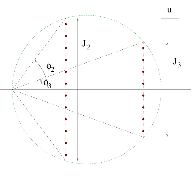
Figure 2: Distribution of momenta in terms of $u_{j}=\frac{1}{2}\cot\frac{k_{j}}{2}$ for the two magnon state. Geometrically, it is interesting that the angles shown are half the momenta of each magnon and also that the center of the circle is at a distance from the origin equal to the inverse of the group velocity (which is the same for both magnons so there is only one circle).

6 Conclusions

We have studied a generalized ansatz for strings moving in $AdS_{5}\times{S}^{5}$ that reduces the problem of finding solutions to that of solving the Neumann-Rosochatius system. That system describes an effective particle moving on a sphere in a specific potential. In our case we had an extra term equivalent to a coupling to a magnetic field. Such term, however, appeared only in the equations for the angular variables. For the radial coordinates, we still got the usual NR lagrangian. After solving the NR system, the trajectory of the particle should be understood as the profile of the string. Such string rotates rigidly in time according to the ansatz we proposed.

Since the solutions of the Neumann-Rosochatius system are relatively simple to find, we extended the giant magnon solution to the case of two additional angular momenta. Although, in principle, the integrability does not guarantee a simple expression for the conserved string quantities (such as angular momenta), we have found a rather simple result: the conserved quantities correspond to a superposition of those of two giant magnons, each carrying one of the two finite angular momenta. However, since the solution turned out to describe a rigid string we got an extra condition that the group velocity of the two magnons should be the same. It would be interesting to study other solutions (which will no longer be described by the NR ansatz) where the two magnons move relatively to each other.

In the weak coupling gauge theory limit the description of the two magnons is that of two bound states in a spin chain that move freely. Here it is trivial to consider the magnons moving with respect to each other since we can see that they do not interact. The wave function of such system can be constructed using the Bethe ansatz as we discussed in some detail.

An interesting point is that, on the string side, using the plots we presented, one can easily differentiate the two magnons. This suggests that one can directly relate the position along the spin chain with the position along the string. It should be interesting to establish a more precise map between the action of the string and that of the spin chain as can be done at small momentum in the “thermodynamic” limit.

Finally, we should note that the ansatz that we used here can be generalized to the full $AdS_{5}\times{S}^{5}$ case (as in [12]); one can also include some pulsating solutions by interchanging the $\sigma$ and $\tau$ world-sheet coordinates. It would be interesting to understand these other solutions and see if there is an analog of the giant magnon solution in those larger sectors.

7 Acknowledgments

We are very grateful to I. Klebanov, J. Minahan, R. Roiban and A. Tirziu for various comments and discussions. M.K. and A.A.T. are also grateful to the KITP at Santa Barbara for hospitality during the 2004 “QCD and Strings” workshop where some of the ideas of this work were conceived.

The work of J.R. and A.A.T. is supported in part by the European EC-RTN network MRTN-CT-2004-005104. J.R. also acknowledges support by MCYT FPA 2004-04582-C02-01. The work of A.A.T. is supported in part by the DOE grant DE-FG02-91ER40690, INTAS 03-51-6346 and the RS Wolfson award. The work of M.K. was supported in part by the National Science Foundation Grant No. PHY-0243680. Any opinions, findings, and conclusions or recommendations expressed in this material are those of the authors and do not necessarily reflect the views of the National Science Foundation.

Note added

While this paper was in preparation, there appeared two papers [33] and [34] which also discuss spinning giant magnons on $S^{5}$. The three-spin solution presented at the end of [33] corresponds to a special case of our solution with energy given by (4.120) and having $s_{1}=0$, $\phi_{2}=\phi_{3}={\pi\over 2}$. At the same time, we do not understand the three-spin solution presented in sect. 2.2 of [34].

References

-
[1]
J. Maldacena,
“The large limit of superconformal field theories and supergravity,”
Adv. Theor. Math. Phys. 2, 231 (1998)
[Int. J. Theor. Phys. 38, 1113 (1998)],
hep-th/9711200,
S. S. Gubser, I. R. Klebanov and A. M. Polyakov, “Gauge theory correlators from non-critical string theory,” Phys. Lett. B 428, 105 (1998) [arXiv:hep-th/9802109],
E. Witten, “Anti-de Sitter space and holography,” Adv. Theor. Math. Phys. 2, 253 (1998) [arXiv:hep-th/9802150],
- [2] G. ’t Hooft, “A Two-Dimensional Model For Mesons,” Nucl. Phys. B 75, 461 (1974).
- [3] D. Berenstein, J. M. Maldacena and H. Nastase, “Strings in flat space and pp waves from N = 4 super Yang Mills,” JHEP 0204, 013 (2002) [arXiv:hep-th/0202021].
- [4] S. S. Gubser, I. R. Klebanov and A. M. Polyakov, “A semi-classical limit of the gauge/string correspondence,” Nucl. Phys. B 636, 99 (2002) [arXiv:hep-th/0204051].
- [5] S. Frolov and A. A. Tseytlin, “Multi-spin string solutions in AdS(5) x S**5,” Nucl. Phys. B 668, 77 (2003) [arXiv:hep-th/0304255]. “Rotating string solutions: AdS/CFT duality in non-supersymmetric sectors,” Phys. Lett. B 570, 96 (2003) [arXiv:hep-th/0306143].
- [6] J. A. Minahan and K. Zarembo, “The Bethe-ansatz for N = 4 super Yang-Mills,” JHEP 0303 (2003) 013 [arXiv:hep-th/0212208].
-
[7]
N. Beisert, J. A. Minahan, M. Staudacher and K. Zarembo,
“Stringing spins and spinning strings,”
JHEP 0309, 010 (2003)
[arXiv:hep-th/0306139],
N. Beisert, S. Frolov, M. Staudacher and A. A. Tseytlin, “Precision spectroscopy of AdS/CFT,” JHEP 0310, 037 (2003) [arXiv:hep-th/0308117]. - [8] M. Kruczenski, “Spin chains and string theory,”, Phy. Rev. Lett 93, 161602 (2004), [arXiv:hep-th/0311203].
- [9] M. Kruczenski, A. V. Ryzhov and A. A. Tseytlin, “Large spin limit of AdS(5) x S**5 string theory and low energy expansion of ferromagnetic spin chains,” Nucl. Phys. B 692, 3 (2004) [arXiv:hep-th/0403120].
-
[10]
V. A. Kazakov, A. Marshakov, J. A. Minahan and K. Zarembo,
“Classical / quantum integrability in AdS/CFT,”
JHEP 0405, 024 (2004)
[arXiv:hep-th/0402207],
N. Beisert, V. A. Kazakov and K. Sakai, “Algebraic curve for the SO(6) sector of AdS/CFT,” Commun. Math. Phys. 263, 611 (2006) [arXiv:hep-th/0410253],
N. Dorey and B. Vicedo, “On the dynamics of finite-gap solutions in classical string theory,” arXiv:hep-th/0601194. - [11] G. Arutyunov, S. Frolov, J. Russo and A. A. Tseytlin, “Spinning strings in AdS(5) x S5 and integrable systems,” Nucl. Phys. B 671, 3 (2003) [arXiv:hep-th/0307191]
- [12] G. Arutyunov, J. Russo and A. A. Tseytlin, “Spinning strings in AdS(5) x S5: New integrable system relations,” Phys. Rev. D 69, 086009 (2004) [arXiv:hep-th/0311004].
-
[13]
C. Neumann,
De problemate quodam mechanico, quod ad primam integralium ultraellipticorum classem revocatur,”
Jour. reine Angew. Math. 56, 1859 pp. 46-63,
E. Rosochatius, “Über Bewegungen eines Punktes,” Dissertation at Univ. Götingen, Druck von Gebr. Unger, Berlin 1877. - [14] J. Moser, “Various aspects of integrable Hamiltonian Systems,” in “Dynamical systems”, Progress in Mathematics 8, C.I.M.E. Lectures, Bressanone, Italy, (1978), J. Coates, S. Helgason, Eds.
- [15] M. Kruczenski, “Spiky strings and single trace operators in gauge theories,” JHEP 0508, 014 (2005) [arXiv:hep-th/0410226].
- [16] S. Ryang, “Wound and rotating strings in AdS(5) x S**5,” JHEP 0508, 047 (2005) [arXiv:hep-th/0503239].
- [17] D. M. Hofman and J. M. Maldacena, “Giant magnons,” arXiv:hep-th/0604135.
- [18] N. Dorey, “Magnon bound states and the AdS/CFT correspondence,” arXiv:hep-th/0604175.
- [19] H. Y. Chen, N. Dorey and K. Okamura, “Dyonic giant magnons,” arXiv:hep-th/0605155.
- [20] G. Arutyunov, S. Frolov and M. Zamaklar, “Finite-size effects from giant magnons,” arXiv:hep-th/0606126.
- [21] J. A. Minahan, A. Tirziu and A. A. Tseytlin, “Infinite spin limit of semiclassical string states,” arXiv:hep-th/0606145.
-
[22]
C. J. Burden,
“Gravitational Radiation From A Particular Class Of Cosmic Strings,”
Phys. Lett. B 164, 277 (1985),
C. J. Burden and L. J. Tassie, “Additional Rigidly Rotating Solutions In The String Model Of Hadrons,” Austral. J. Phys. 37, 1 (1984). - [23] J. A. Minahan, “Circular semiclassical string solutions on AdS(5) x S**5,” Nucl. Phys. B 648, 203 (2003) [arXiv:hep-th/0209047].
- [24] M. Kruczenski and A. A. Tseytlin, “Semiclassical relativistic strings in S5 and long coherent operators in N = 4 SYM theory,” JHEP 0409, 038 (2004) [arXiv:hep-th/0406189].
-
[25]
V. M. Braun, S. E. Derkachov and A. N. Manashov,
“Integrability of three-particle evolution equations in QCD,”
Phys. Rev. Lett. 81, 2020 (1998)
[arXiv:hep-ph/9805225],
V. M. Braun, S. E. Derkachov, G. P. Korchemsky and A. N. Manashov, “Baryon distribution amplitudes in QCD,” Nucl. Phys. B 553, 355 (1999) [arXiv:hep-ph/9902375],
A. V. Belitsky, “Integrability and WKB solution of twist-three evolution equations,” Nucl. Phys. B 558, 259 (1999) [arXiv:hep-ph/9903512]; “Fine structure of spectrum of twist-three operators in QCD,” Phys. Lett. B 453, 59 (1999) [arXiv:hep-ph/9902361]. - [26] R. Hernandez and E. Lopez, “The SU(3) spin chain sigma model and string theory,” JHEP 0404, 052 (2004) [arXiv:hep-th/0403139].
- [27] C.N. Yang, “Some Exact Results For The Many Body Problems In One Dimension With Repulsive Delta Function Interaction,” Phys. Rev. Lett. 19, 1312 (1967).
- [28] B. Sutherland, “An introduction to the Bethe ansatz”, in “Exactly Solvable Problems in Condensed Matter and Relativistic Field Theory”, Lecture Notes in Physics 242, Springer-Verlag, Berlin Heidelberg (1985).
-
[29]
J. Engquist, J. A. Minahan and K. Zarembo,
“Yang-Mills duals for semiclassical strings on AdS(5) x S**5,”
JHEP 0311, 063 (2003)
[arXiv:hep-th/0310188],
C. Kristjansen, “Three-spin strings on AdS(5) x S**5 from N = 4 SYM,” Phys. Lett. B 586, 106 (2004) [arXiv:hep-th/0402033],
L. Freyhult, “Bethe ansatz and fluctuations in SU(3) Yang-Mills operators,” JHEP 0406, 010 (2004) [arXiv:hep-th/0405167],
C. Kristjansen and T. Mansson, “The circular, elliptic three-spin string from the SU(3) spin chain,” Phys. Lett. B 596, 265 (2004) [arXiv:hep-th/0406176]. - [30] B. J. Stefanski and A. A. Tseytlin, “Large spin limits of AdS/CFT and generalized Landau-Lifshitz equations,” JHEP 0405, 042 (2004) [arXiv:hep-th/0404133].
- [31] H. Bethe, “On The Theory Of Metals. 1. Eigenvalues And Eigenfunctions For The Linear Atomic Chain,” Z. Phys. 71, 205 (1931).
- [32] N. Beisert, V. Dippel and M. Staudacher, “A novel long range spin chain and planar N = 4 super Yang-Mills,” JHEP 0407, 075 (2004) [arXiv:hep-th/0405001].
- [33] M. Spradlin and A. Volovich, “Dressing the Giant Magnon,” arXiv:hep-th/0607009.
- [34] N. P. Bobev and R. C. Rashkov, “Multispin Giant Magnons,” arXiv:hep-th/0607018.