Trapped Quintessential Inflation in the context of Flux Compactifications

Abstract

We present a model for quintessential inflation using a string modulus for the inflaton - quintessence field. The scalar potential of our model is based on generic non-perturbative potentials arising in flux compactifications. We assume an enhanced symmetry point (ESP), which fixes the initial conditions for slow-roll inflation. When crossing the ESP the modulus becomes temporarily trapped, which leads to a brief stage of trapped inflation. This is followed by enough slow roll inflation to solve the flatness and horizon problems. After inflation, the field rolls down the potential and eventually freezes to a certain value because of cosmological friction. The latter is due to the thermal bath of the hot big bang, which is produced by the decay of a curvaton field. The modulus remains frozen until the present, when it becomes quintessence.

1 Introduction

An array of recent observations has ascertained that we live in a Universe which is engaging into accelerated expansion at present [1]. The simplest explanation for this observation is to assume a non-zero cosmological constant, corresponding to vacuum energy density comparable to the density of matter today. However, such a value for the cosmological constant is extremely fine-tuned compared to theoretical expectations [2]. As a result, a number of alternatives has been suggested in the literature. Many of the alternative solutions postulate the existence of an unknown exotic substance, called Dark Energy, whose properties (e.g. equation of state) are such that it would drive the Universe to accelerated expansion if it dominates the Universe content (for a recent review see [3]). A particular type of such substance, which fulfils the requirements of dark energy is a potentially dominated scalar field. Under this hypothesis, the cosmological constant may be set to zero, as once assumed, so that the extreme fine-tuning of its value can be avoided. This means that the scalar field either lies at a metastable minimum of the scalar potential or is rolling down a slope in the scalar potential leading to the minimum, which corresponds to zero density. This latter case has been envisaged some time ago in models of ‘dynamical cosmological constant’ [4]. With respect to accounting for dark energy, the scalar field has been named ‘quintessence’ because it is the fifth element after baryons, photons, CDM and neutrinos [5].

The idea of using a rolling scalar field in order to achieve a phase of accelerated expansion in the Universe history is, of course, not new. In fact, it is the basis of the inflationary paradigm, where the scalar field is the so-called ‘inflaton’ [6]. Hence, quintessence corresponds to nothing more than a late time inflationary period, taking place at present. In this respect, the credibility of the quintessence idea has been enhanced by the fact that the generic predictions of the inflationary paradigm in the Early Universe are very much in agreement with the observations.

Since they are based on the same idea, it was natural to attempt to unify early Universe inflation with quintessence. Quintessential inflation was thus born [7, 8, 9, 10]. The advantages of such unified models are many. Firstly, quintessential inflation models allow the treatment of both inflation and quintessence within a single theoretical framework, with hopefully fewer and more tightly constrained parameters. Another practical gain is the fact that quintessential inflation dispenses with a tuning problem of quintessence models; that of the initial conditions for the quintessence field. It is true that attractor - tracker quintessence alleviates this tuning but the problem never goes away completely. In contrast, in quintessential inflation the initial conditions for the late time accelerated expansion are fixed in a deterministic manner at the end of inflation. Finally, a further advantage of unified models for inflation and quintessence is the economy of avoiding to introduce yet again another unobserved scalar field to explain the late accelerated expansion.

For quintessential inflation to work one needs a scalar field with a runaway potential, such that the minimum has not been reached until today and, therefore, there is residual potential density, which, if dominant, can cause the observed accelerated expansion. String moduli fields appear suitable for this role because they are typically characterised by such runaway potentials. The problem with such fields, however, is how to stabilise them temporarily, in order to use them as inflatons in the early Universe.

In this paper (see also Ref. [11]) we achieve this by considering that, during its early evolution our modulus crosses an enhanced symmetry point (ESP) in field space. As shown in Ref. [12], when this occurs the modulus may be trapped at the ESP for some time. This can lead to a period of inflation, typically comprised by many sub-periods of different types of inflation such as trapped, eternal, old, slow-roll, fast-roll and so on. After the end of inflation the modulus picks up speed again in field space resulting into a period of kinetic density domination, called ‘kination’ [13]. Kination is terminated when the thermal bath of the hot big bang (HBB) takes over. During the HBB, due to cosmological friction [14], the modulus freezes asymptotically at some large value and remains there until the present, when its potential density becomes dominant and drives the late-time accelerated expansion [10].

Is is evident that, in order for the scalar field to play the role of quintessence, it should not decay after the end of inflation. Reheating, therefore should be achieved by other means. In this paper we assume that the thermal bath of the HBB is due to the decay of some curvaton field [15] as suggested in Refs. [16]. Note that the curvaton can be a realistic field, already present in simple extensions of the standard model (for example it can be a right-handed sneutrino [17], a flat direction of the MSSM and its extensions [18, 19] or a pseudo Nambu-Goldstone boson [20, 21] possibly associated with the Peccei-Quinn symmetry [22] etc.). Thus, by considering a curvaton we do not necessarily add an ad hoc degree of freedom. The importance of the curvaton lies also in the fact that the energy scale of inflation can be much lower than the grand unified scale [23]. In fact, in certain curvaton models, the Hubble scale during inflation can be as low as the electroweak scale [21, 24].

Throughout our paper we use natural units, where $c=\hbar=1$ and Newton’s gravitational constant is $8\pi G=m_{P}^{-2}$, with $m_{P}=2.4\times 10^{18}$GeV being the reduced Planck mass.

2 Field dynamics at an ESP

String theory compactifications possess distinguished points in their moduli space at which some massive states of the theory become massless. This often results in the enhancement of the gauge symmetries of the theory [25]. However, this enhancement does not persist when the field moves away from the point of symmetry, and therefore, such points can be associated with symmetry breaking processes [26], and with a string theoretical Higgs effect leading to moduli stabilisation [27].

Even though from the classical point of view an enhanced symmetry point (ESP) is not a special point, as a field approaches it certain states in the string spectrum become massless [27]. In turn, these massless modes create an interaction potential that may drive the field back to the symmetry point. In this sense, quantum effects make the ESP a preferred location in field space.

With respect to the properties of the scalar potential, we have that the ESPs are dynamical attractors for the action of the fields. Therefore the scalar potential is flat at these points

$$V^{\prime}_{0}\equiv V^{\prime}(\phi_{0})=0\,,$$ (1)

where the prime denotes derivative with respect to the modulus $\phi$, and $\phi_{0}$ denotes the position of the ESP. In Ref. [28], the authors consider that the presence of the ESP generates and extremum in the scalar potential. In particular, both a maximum and a minimum are jointly considered (requiring the presence of two ESPs). In this paper we study the case of a single symmetry point, and consider the cases when the ESP results in a flat inflection point and in a local extremum.

2.1 Particle production at an ESP

The Lagrangian of the system for the case of two real scalar fields $\phi$ and $\chi$ is [12]

$${\cal L}=\frac{1}{2}\,\partial_{\mu}\phi\partial^{\mu}\phi+\frac{1}{2}\,\partial_{\mu}\chi\partial^{\mu}\chi-V(\phi)-V_{\rm int}(\phi,\chi)\,,$$ (2)

where

$$V_{\rm int}(\phi,\chi)\equiv\frac{1}{2}\,g^{2}\chi^{2}\phi^{2}$$ (3)

and $g$ is a dimensionless coupling. The effective masses for the fields $\chi$ and $\phi$ are

$$m^{2}_{\chi}=g^{2}\phi^{2}\quad,\quad m^{2}=m_{\phi}^{2}+g^{2}\chi^{2}\,,$$ (4)

where $m_{\phi}^{2}\equiv V^{\prime\prime}(0)$. For simplicity, and until Sec. 3, we take $V(\phi)$ as approximately constant and equal to $V_{0}\equiv V(0)$ in the region of interest around the ESP. Also, we write

$$V_{0}\equiv 3H_{*}^{2}m_{P}^{2}\,,$$ (5)

where $H_{*}$ is a constant mass scale equal to the Hubble scale during inflation.

If $\phi$ moves towards the symmetry point, then $m_{\chi}^{2}$ changes with time. This time-dependent mass leads to the creation of particles with momentum $k\lesssim(g\dot{\phi}_{0})^{1/2}$, where $\dot{\phi}_{0}$ denotes the velocity of $\phi$ in field space at the location of the ESP $\phi_{0}=0$. The production takes place when the field is within the production window [12]

$$|\phi|<\Delta\phi\sim(\dot{\phi}_{0}/g)^{1/2},.$$ (6)

After the first production event, the expectation value $\langle\chi^{2}\rangle$ is

$$\langle\chi^{2}\rangle\simeq\frac{1}{2\pi^{2}}\int_{0}^{\infty}\frac{n_{k}^{(1)}\,k^{2}dk}{\sqrt{k^{2}+g^{2}\phi^{2}}}\simeq\frac{n_{\chi}^{(1)}}{g|\phi|}$$ (7)

when $\phi$ is outside the production window. The occupation number after the first crossing is $n_{k}^{(1)}=\exp(-\pi k^{2}/g\dot{\phi}_{0})$ [29]. The density of $\chi$ particles grows then to $n_{\chi}^{(1)}\sim g^{3/2}\dot{\phi}_{0}^{3/2}$, and the field moves in the linear potential

$$V_{\rm eff}(\phi)\sim V(\phi_{0})+gn_{\chi}^{(1)}|\phi|\,.$$ (8)

The field climbs up the linear potential until it reaches a turning point, at a distance $\Phi_{1}\sim g^{-5/2}\dot{\phi}_{0}^{1/2}$. The field then bounces back towards the ESP, where a new production event occurs. The interaction potential is then reinforced by the newly created particles, and, after leaving again the production window, the field bounces back this time at a distance $\Phi_{2}<\Phi_{1}$. The process continues until the turning point is at a distance from the ESP comparable to the production window, i.e. $\Phi\sim\Delta\phi$; once this point is reached, it can be considered that no more particles are produced. The final number density of $\chi$ particles created throughout the whole process is $n_{\chi}\sim g^{-1/2}\dot{\phi}_{0}^{3/2}$ [12].

The picture we just described is simplistic, since once it crosses the ESP, the field is always forced to fall back to the symmetry point regardless of how far away is the first turning point $\Phi_{1}$ from the symmetry point. However, in a more realistic case, in order to avoid the overshoot problem we have to impose the condition

$$\Phi_{1}\sim g^{-5/2}\dot{\phi}_{0}^{1/2}<m_{P}\,,$$ (9)

since for larger distances in field space the coupling softens and the field, instead of falling back to the symmetry point, would keep rolling down its potential [30].

2.2 Post-production evolution

We take into account now the expansion of the Universe, and keep assuming that the scalar potential $V(\phi)$ is flat enough not to disturb the dynamics dictated by $V_{\rm int}(\phi)$.

When particle production finishes, the mass term $m_{\chi}^{2}=g^{2}\phi^{2}$ no longer dominates over $k^{2}$ in Eq. (7). The $\chi$ particles then become relativistic, and their energy is depleted as $a^{-4}$ by the expansion of the Universe. Moreover, we can write $\sqrt{k^{2}+g^{2}\phi^{2}}\sim k$, which means that $\langle\chi^{2}\rangle$ becomes $\phi$-independent. At the end of particle production, for which we set $a=1$, the field then oscillates in the quadratic potential

$$V_{\rm int}(\phi)=g^{2}\langle\chi^{2}\rangle\phi^{2}\sim(g\dot{\phi}_{0})\phi^{2}\,.$$ (10)

Here we state the main results concerning the evolution of the field $\phi$ and the expectation value $\langle\chi^{2}\rangle$, reserving the technical details of the computation for appendix 9.1. In this appendix we find that, as long as $m^{2}\gtrsim H^{2}$, the amplitude of oscillations $\Phi$ and the expectation value $\langle\chi^{2}\rangle$ are given by

$$\displaystyle\Phi(t)=\frac{\Phi_{a=1}}{a}\sim\frac{\Delta\phi}{a}\,,$$ (11)

$$\displaystyle\langle\overline{\chi^{2}}(t)\rangle=\frac{\langle\overline{\chi^{2}}\rangle_{a=1}}{a^{2}}\sim\frac{g^{-1}\dot{\phi}_{0}}{a^{2}}=\Phi^{2}(t)\,,$$ (12)

From the above, it is evident that the density of $\phi$ stored in the oscillations around the ESP is depleted as

$$\rho_{\rm osc}=V_{\rm int}(\Phi)\propto a^{-4}\,.$$ (13)

We also stress that as long as the oscillation energy dominates the total density, the ratio $m^{2}/H^{2}$, where $m^{2}\approx g^{2}\langle\overline{\chi^{2}}\rangle$, grows as the Universe expands, $m^{2}/H^{2}\propto\langle\overline{\chi^{2}}\rangle/\rho_{\rm osc}\propto a^{2}$.

When the kinetic density of the oscillating field falls below the potential density $V_{0}$, a phase of inflation called trapped inflation begins [12]. Taking into account the depletion rates given by Eqs. (11) and (13), trapped inflation commences at $a\sim(\dot{\phi}_{0}^{2}/V_{0})^{1/4}$. Using Eq. (11), the amplitude of oscillation is

$$\Phi_{i}\sim(g^{-1}H_{*}m_{P})^{1/2}\,.$$ (14)

From this moment on $H$ becomes approximately equal to $H_{*}$, and the field starts to decrease its rate of oscillation $m^{2}/H^{2}\sim g^{2}\langle\overline{\chi^{2}}\rangle/H_{*}^{2}\propto a^{-2}$. Owing to this decrease, the phase of oscillations will finish when the expansion of the Universe starts to overdamp the oscillations of the field, which happens when $m^{2}/H_{*}^{2}\sim 1$. The field then reaches its minimum amplitude of oscillations. Using Eq. (12), this is given by

$$\Phi_{\rm min}\sim H_{*}/g\,.$$ (15)

The amount of inflation during the phase of oscillations is then

$$N_{\rm osc}=\ln\frac{\Phi_{i}}{\Phi_{\rm min}}\sim\ln\left[g^{1/2}\left(\frac{m_{P}}{H_{*}}\right)^{1/2}\right]\,.$$ (16)

Note that $N_{\rm osc}$ is independent of the initial value $\dot{\phi}_{0}$. This is because the kinetic density in excess of $V_{0}$ must be exhausted before trapped inflation can begin. Therefore, we find the same amount of inflation if we take $\dot{\phi}_{0}^{2}\sim V_{0}$ and set the beginning of trapped inflation at $a=1$, which corresponds to suppressing the interphase in which the excess of kinetic density is depleted. Hence, the only scale relevant here is $H_{*}$.

Once the phase of oscillation is over, the depletion rates computed in Eqs. $(\ref{eq:evolution1})$ and $(\ref{eq:evolution2})$ no longer apply. The expansion of the Universe now makes the mass of the field fall below $H_{*}$, and a phase of slow-roll inflation follows. We emphasize that this phase of slow-roll occurs with the field rolling down the interaction potential $V_{\rm int}(\phi)$. When the expansion of the Universe has redshifted sufficiently the kinetic density of the field, the motion of the later ceases to be classical to become dominated by the vacuum fluctuation of the field. A phase of eternal inflation then follows. We devote the rest of this section to study in detail this transient to the phase of eternal inflation.

2.3 Towards eternal inflation

When the mass of the field falls below $H_{*}$ after the end of the oscillatory phase, the field begins to slow-roll over the interaction potential. The equation of motion is

$$3H\dot{\phi}\simeq-V_{\rm int}^{\prime}(\phi)\,,$$ (17)

and the classical motion of the field $\Delta\phi_{c}$ per Hubble time is

$$\Delta\phi_{\rm c}\sim\dot{\phi}/H_{*}\simeq-\frac{V_{\rm int}^{\prime}(\Phi_{\rm min})}{3H_{*}^{2}}\,,$$ (18)

Using the estimate above we can compare the classical motion $\Delta\phi_{c}$ with $|\phi|\lesssim\Phi_{\rm min}$ at the beginning of slow-roll, obtaining

$$\frac{|\Delta\phi_{c}|}{\Phi_{\rm min}}\sim\frac{|V_{\rm int}^{\prime}|}{H_{*}^{2}}\frac{1}{\Phi_{\rm min}}\sim\frac{g^{2}\langle\chi^{2}\rangle|\phi|}{H_{*}^{2}\,\Phi_{\rm min}}<1\,,$$ (19)

which follows from the slow-roll condition $|\eta|<1$. Therefore, the value $|\phi|$ after the end of oscillations remains within the order of $\Phi_{\rm min}$, and roughly constant during a Hubble time $|\phi|\lesssim\Phi_{\rm min}$. Moreover, given that both the kinetic term $k^{2}$ and the mass term $g^{2}\Phi^{2}$ in $\langle\overline{\chi^{2}}\rangle$ [c.f. Eq. (7)] remain comparable until the end of oscillations, the mass term starts to dominate over the kinetic term soon after the onset of the slow-roll phase. Consequently, the $\chi$ particles become again non-relativistic. Indeed,

$$\langle\chi^{2}\rangle\sim\int_{0}^{\infty}\frac{n_{k}(t)\,k^{2}dk}{\sqrt{k^{2}+g^{2}\phi^{2}}}\ \propto\frac{n_{\chi}}{|\phi|}\propto a^{-3}\,.$$ (20)

This result allows us to obtain the decrease rate of both the slope $V^{\prime}_{\rm int}(\phi)\propto a^{-3}$ and the effective mass squared $m^{2}\propto a^{-3}$. The scaling law for the kinetic density of the field

$$\rho_{\rm kin}=\frac{1}{2}\,\dot{\phi}^{2}\simeq\frac{1}{2}\left(\frac{V_{\rm int}^{\prime}}{3H}\right)^{2}\propto a^{-6}\,,$$ (21)

which may be compared to the milder rate that applies when $\phi$ oscillates, Eq. (13).

Now we compute the amount of slow-roll inflation during the transient to eternal inflation. Owing to rapid redshift of the effective mass and to the very slow-roll motion of the field, we assume that $|\phi|$ remains within the order of $\Phi_{\rm min}$.

The slow-roll motion of the field begins when $m^{2}\sim H_{*}$, and persists until

$$|V^{\prime}_{\rm int}|\sim H_{*}^{3}\,.$$ (22)

Using that $|V^{\prime}_{\rm int}|\sim H_{*}^{3}/g$ at the beginning of the slow-roll and that $V^{\prime}_{\rm int}\propto a^{-3}$, the amount of slow-roll inflation during the transient to eternal inflation is

$$N_{\rm sr}\sim\frac{1}{3}\ln\frac{1}{g}\,.$$ (23)

Taking for example $g\simeq 0.1$ this gives $N_{\rm sr}\sim 1$, which is a negligible amount. The assumption $|\phi|\sim\Phi_{\rm min}$ is indeed correct.

Once $|V^{\prime}_{\rm int}|$ falls below $H_{*}^{3}$, the field becomes dominated by its vacuum fluctuation. The field then performs a random motion taking steps of amplitude $\delta\phi\sim H_{*}/2\pi$ every Hubble time. The motion of the field during this phase is oblivious of the scalar potential and is only known probabilistically, with the root mean square of the field growing to $\sqrt{\langle\phi^{2}\rangle}\sim\frac{H_{*}}{2\pi}\sqrt{N}$ after $N$ $e$-foldings of eternal inflation [32]. The number of $e$-foldings of trapped inflation is therefore well approximated by Eq. (16). In view of this result we emphasize that, as far as trapped inflation in concerned, the main virtue of the trapping mechanism does not rely on its capacity to produce inflation, but in that it sets the field at a locally flat region in field space. Therefore, depending upon the strength of the symmetry point, this mechanism may fix the initial conditions leading to a subsequent long-lasting stage of inflation.

Up until now we have assumed that the scalar potential $V(\phi)$ plays no role in the dynamics of the field, apart from contributing $V_{0}$. We now address the complete picture where a non-trivial ‘background’ scalar potential $V(\phi)$ is present.

3 String inspired quintessential inflation

Type IIB compactifications have received a great deal of attention due to recent accomplishments in moduli stabilisation [33]. The integrated contribution of the fluxes induces a non-zero superpotential, $W=W_{0}$. Assuming that this contribution is independent of the fields leads to no-scale supergravity, in which the Kähler moduli remain exactly flat. However, these flat directions can be lifted up through non-perturbative effects, such as gaugino condensation or D-brane instantons [34]. In this case, the superpotential $W$ takes the form

$$W=W_{0}+W_{\rm np}\quad\textrm{with}\quad W_{\rm np}=Ae^{-cT}\,,$$ (24)

where $W_{0}$ is the tree level contribution from fluxes, $A$ and $c$ are constants, whose magnitude and physical interpretation depends on the origin of the non-perturbative term (in the case of gaugino condensation $c$ is expected to take on values $c\lesssim 1$), and $T$ is a Kähler modulus in units of $m_{P}$, for which

$$T=\sigma+i\alpha\,.$$ (25)

with $\sigma$ and $\alpha$ real. The inclusion of the non-perturbative superpotential $W_{\rm np}$ results in a runaway scalar potential characteristic of string compactifications. In type IIB compactifications with a single Kähler modulus, this is the so-called volume modulus. In this case, the runaway behaviour leads to decompactification of the internal manifold.

The tree level Kähler potential for the a modulus, written in units of $m_{P}^{2}$, is

$$K=-3\,\textrm{ln}\,(T+\bar{T})\,,$$ (26)

and the corresponding supergravity potential is

$$V_{\rm np}(\sigma)=\frac{cAe^{-c\sigma}}{2\sigma^{2}m_{P}^{2}}\left[\left(1+\frac{c\sigma}{3}\right)Ae^{-c\sigma}+W_{0}\cos(c\alpha)\right]\,.$$ (27)

To secure the validity of the supergravity approximation we consider $\sigma>1$. For values of $c\lesssim 1$, we then have $c\sigma>1$. To account now for the ESP, we consider that the scalar potential $V_{\rm np}(\phi)$ receives a phenomenological contribution $V_{\rm ph}(\sigma)$ important only in the neighbourhood of the ESP. Therefore, we consider the scalar potential

$$V(\sigma)=V_{\rm np}(\sigma)+V_{\rm ph}(\sigma)$$ (28)

as long as the field is close to the ESP, whereas we consider $V(\sigma)\approx V_{\rm np}(\sigma)$ when the field is sufficiently away from it. By choosing $V_{\rm ph}(\sigma)$ appropriately it is possible to account for an ESP with $dV/d\sigma=0$ at $\sigma_{0}$. The field may thus drive a period of inflation when close to $\sigma_{0}$. In order to study the arising inflationary dynamics, we turn to the canonically normalized field $\phi$ associated to $\sigma$. Owing to Eq. (26) we have

$$\sigma(\phi)=\textrm{exp}\,(\sqrt{2/3}\,\phi/m_{P})\,.$$ (29)

In appendix 9.2 we show how, within our phenomenological approach, the inflationary dynamics may be fully accounted for through the scalar potential

$$V(\phi)=V_{0}+\frac{1}{2}m_{\phi}^{2}\bar{\phi}^{2}+\frac{1}{3!}V_{0}^{\textrm{\tiny(3)}}\bar{\phi}^{3}\,,$$ (30)

where we have defined

$$\bar{\phi}\equiv\phi-\phi_{0}\,.$$ (31)

Also, with the symmetry point located at $\phi_{0}$, the interaction potential becomes now $V_{\rm int}(\phi)=\frac{1}{2}g^{2}\chi^{2}\bar{\phi}^{2}$. The free parameters of the scalar potential $V(\phi)$ are $H_{*}$, $m_{\phi}^{2}$ and $V_{0}^{\textrm{\tiny(3)}}$. Within our minimal approach, $V_{0}^{\textrm{\tiny(3)}}$ is determined by $H_{*}$, which sets the height of the potential at the ESP, and by how close to the symmetry point the potential $V_{\rm ph}(\sigma)$ becomes exponentially suppressed with respect to $V_{\rm np}(\sigma)$ (see Appendix 9.2). In our model we allow these two parameters to vary independently. Also, the sign of $V_{0}^{\textrm{\tiny(3)}}$ is always negative, whereas $m_{\phi}^{2}$ may be positive, negative, or effectively zero if the quadratic term in $V(\phi)$ is subdominant with respect to the cubic one. These three cases are pictured in Fig 1.

If the ESP results in a maximum, the field may grow to large values when the field breaks free from its trapping even if the quadratic term dominates $V(\phi)$. Nonetheless, if the quadratic term dominates there is still a chance that the field is stabilised in the neighbouring minimum. On the contrary, an ESP resulting in a minimum always leads to stabilisation if the quadratic term dominates $V(\phi)$ when the field breaks free. In such a case the field drives a period of old inflation [6]. Once the field tunnels the barrier, it continues rolling down its potential.

Stabilisation when the ESP results in a minimum is considered in Ref. [35], where the suggestion is made of stabilising all of the moduli fields at points of enhanced symmetry (see also Ref. [36] for a more recent study of stabilisation at an ESP). In contrast to these cases, the ESP considered in our approach just provides an effective ground state unstable through tunneling.

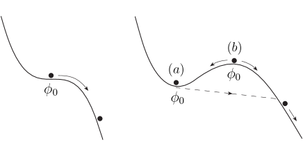
Figure 1: The left panel shows the scalar potential $V(\phi)$ around an enhanced symmetry point (ESP) at $\phi_{0}$ and with a subdominant quadratic term. The right panel shows the formation of either a minimum, case (a), or a maximum, case (b). If the ESP results in a minimum the field accesses the large field region through quantum tunneling. We assume that after tunneling the field appears at approximately the same height. If the ESP results in a maximum, the field may fall towards the minimum or continue rolling towards large values.

4 Inflationary dynamics

4.1 Inflationary regimes

In Sec. 2 we assumed that $V(\phi)$ is flat enough to allow the field to progress ultimately to the phase of eternal inflation under only the influence of the interaction potential $V_{\rm int}$. In general, however, the scalar potential $V(\phi)$ may start to drive the dynamics at any moment after the end of particle production. This happens when

$$|V^{\prime}(\Phi)|\sim V_{\rm int}^{\prime}(\Phi)\,.$$ (32)

From that moment onwards the field breaks free from its trapping and continues rolling over the scalar potential $V(\phi)$. The subsequent evolution of the field may be readily classified in terms of the quantity

$$f(g)\equiv\left|g\frac{m_{\phi}^{2}}{3H_{*}^{2}}+\frac{1}{2}\frac{V_{0}^{\textrm{\tiny(3)}}}{\sqrt{3}H_{*}}\right|\,.$$ (33)

We find the following cases:

Case 1: The field breaks free during the period of fast oscillations following particle production. This corresponds to $|V^{\prime}(\Phi_{\rm min})|>V^{\prime}_{\rm int}(\Phi_{\rm min})$, i.e. $V(\phi)$ controls the dynamics of the field before the latter ceases to oscillate at $|\bar{\phi}|\sim\Phi_{\rm min}$. Using Eq. (30), this condition translates into

$$g<f(g)\,.$$ (34)

In this case, the field is unable to drive a sufficiently long-lasting period of inflation.

Case 2: The field escapes from its trapping at the end of the oscillations. This corresponds to $|V^{\prime}(\Phi_{\rm min})|\sim V^{\prime}_{\rm int}(\Phi_{\rm min})$, which translantes into

$$f(g)\sim g\,.$$ (35)

If $V^{\prime\prime}(\phi)$ does not increase significantly away from the ESP, the field may drive a limited period of inflation, known as fast-roll inflation [37].

Case 3: The field breaks free during the short phase of slow-roll following the end of oscillations. In order to avoid that the field becomes driven by its vacuum fluctuation, we must impose the lower bound $H_{*}^{3}\lesssim V^{\prime}(\Phi_{\rm min})$. This case thus corresponds to

$$g^{2}\lesssim f(g)<g\,.$$ (36)

The slow-roll parameters when the field starts to roll over the scalar potential $V(\phi)$ are $\varepsilon\ll 1$ and $\eta<1$, and hence the field continues its slow-roll motion when released from its trapping. This case may result in enough slow-roll inflation to solve the flatness and horizon problems.

Case 4: The motion of the field is dominated by its vacuum fluctuation. In this case, the field goes through the short phase of slow-roll and then starts to drive eternal inflation. From this stage onwards, the interaction potential becomes very redshifted, playing no role in the dynamics of the field any longer. The field then finds itself at a very flat patch of the scalar potential $V(\phi)$ and driven by its vacuum fluctuation. The field performs a random motion taking steps of amplitude $\delta\phi\sim H_{*}$, and the root mean square of the displaced field grows as $\sqrt{\langle\bar{\phi}^{2}\rangle}\sim NH_{*}$ [32]. This case happens for

$$f(g)<g^{2}\,.$$ (37)

With time, in some parts of the Universe the displaced field grows large, and the steepness of the scalar potential $V(\phi)$ increases. When $V(\phi)$ becomes steep enough the field recovers its classical motion. Eternal inflation then finishes and a long-lasting phase of slow-roll inflation follows. This final phase of slow-roll inflation may be long enough as to solve the flatness and horizon problems as well.

In other parts of the Universe, though, the displaced field always remains in the very flat region. The field never recovers its classical motion, and so it continues driving a never-ending phase of inflation.

4.2 Parameter space for observable inflation

We focus first on the inflationary regimes able to produce enough slow-roll inflation to solve the flatness and horizon problems. In general, the inflationary regimes able to do that provide a number of slow-roll $e$-foldings far larger than the required by observation. However, we only focus on the observable amount of inflation. Also, we allow the observed value of the curvature perturbation to be generated, either partially or entirely, by a scalar field other than the inflaton. The only condition to allow this is that the curvature perturbation generated by the inflaton field, which we denote by ${\cal P}_{\phi}^{1/2}$, is not excessive. The CMB normalization of the spectrum of inflaton perturbations: ${\cal P}_{\phi}^{1/2}\simeq 5\times 10^{-5}$ [38], then becomes a bound [23]

$${\cal P}_{\phi}^{1/2}\lesssim 10^{-5}\,.$$ (38)

As explained in Sec. 3 , the inflationary dynamics in our phenomenological approach can be fully described through the scalar potential in Eq. (30). In this kind of potential, the number of $e$-foldings may be well approximated by taking the end of inflation in the limit $\bar{\phi}(|\eta|\sim 1)\to\infty$. Using the slow-roll formula [38] in this limit, we obtain $\bar{\phi}$ when cosmological scales leave the horizon $N$ $e$-foldings before the end of inflation

$$\bar{\phi}=\frac{m^{2}}{|V_{0}^{\textrm{\tiny(3)}}|}+\frac{|m^{2}|}{|V_{0}^{\textrm{\tiny(3)}}|}\coth(N|\eta|/2)\,.$$ (39)

The curvature perturbation generated by the inflaton field is

$${\cal P}^{1/2}_{\phi}=\frac{1}{2}\frac{N^{2}|V_{0}^{\textrm{\tiny(3)}}|}{\sqrt{3}H_{*}}\left(\frac{\sinh(N|\eta|/2)}{N|\eta|/2}\right)^{2}\approx\frac{1}{2}\frac{N^{2}|V_{0}^{\textrm{\tiny(3)}}|}{\sqrt{3}H_{*}}\,,$$ (40)

where the last follows from the slow-roll condition $|\eta|<1$, and typical values are $N=45-60$. This equation determines $V_{0}^{\textrm{\tiny(3)}}$ in terms of $H_{*}$ and ${\cal P}_{\phi}^{1/2}$. The advantage of this change, apart from the clearer physical meaning of ${\cal P}_{\phi}^{1/2}$, is that Eq. (38) allows us to pick out easily the parameter space leading to an acceptable inflationary cosmology. Also, because in our phenomenological approach $V_{0}^{\textrm{\tiny(3)}}$ has a lower bound at fixed $H_{*}$ (see Appendix 9.2 ), so has ${\cal P}_{\phi}^{1/2}$. Therefore, ${\cal P}_{\phi}^{1/2}$ takes on values in the interval

$$N^{2}(c\sigma_{0})^{3}\frac{H_{*}}{m_{P}}<{\cal P}_{\phi}^{1/2}\lesssim 10^{-5}\,.$$ (41)

Consistency of this inequality sets a maximum value for $H_{*}$, thus resulting in an upper bound for the inflationary scale

$$V_{0}^{1/4}\lesssim 10^{12}\textrm{ GeV}\,,$$ (42)

where we have taken $c\sigma_{0}\sim 10$ and $N=60$. The bound is saturated when the curvature perturbation is generated by the inflaton.

Now, in order to determine what inflationary regimes can be realised in our model, we must find out if they are compatible with the field being trapped. Note that in all the previous discussion to identify the different inflationary regimes, we have implicitly assumed that the field is trapped in the interaction potential $V_{\rm int}(\phi)$. Nonetheless, this might not be the case, hence it is then crucial to determine the interval of $g$ leading to trapping.

To secure that the field is trapped after crossing the ESP, it suffices to require that the scalar potential $V(\phi)$, apart from contributing $V_{0}$, plays no role in the dynamics during particle production. Owing to the decreasing amplitude of oscillations during this process, it is enough to demand $|V^{\prime}(\Phi_{1})|<|V_{\rm int}^{\prime}(\Phi_{1})|$, where $\Phi_{1}$ is the first turning point of the oscillation (see Eq. (9)). This condition translates into

$$g^{10}>\frac{m_{\phi}^{2}}{m_{P}^{2}}+\frac{H_{*}}{m_{P}}N^{-2}{\cal P}_{\phi}^{1/2}\,,$$ (43)

where we have used $|V^{\prime}_{\rm int}(\Phi_{1})|\sim gn_{\chi}^{(1)}$ [c.f. Eq. (8)], and Eq. (40). Using now the lower bound in Eq. (41) and the slow-roll condition $|\eta|<1$ (which requires $m_{\phi}^{2}<H_{*}^{2}$), the first term on the right-hand side becomes negligible. The values of $g$ leading to trapping are thus given by

$$g^{10}\left(\frac{m_{P}}{H_{*}}\right)>N^{-2}{\cal P}_{\phi}^{1/2}\,.$$ (44)

Taking for example the upper bound found in Eq. (42) and ${\cal P}_{\phi}^{1/2}\sim 10^{-5}$, we obtain $g>10^{-2}$. It is also clear that if ${\cal P}_{\phi}^{1/2}$ and $H_{*}$ decrease, so does the lower bound for $g$, thus widening the range of values leading to trapping. Using for example the lower bound in Eq. (41) we obtain $g>(H_{*}/m_{P})^{1/5}$.

Let us study first the case $m_{\phi}^{2}\leq 0$, i.e. the ESP results in either a maximum or a flat inflection point. The results are pictured in Figure 2.

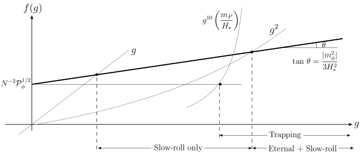
Figure 2: The figure shows the intervals in the $g$-axis corresponding to the two inflationary regimes in terms of the parameters ${\cal P}_{\phi}^{1/2},m_{\phi}^{2}$ and $H_{*}$ for $m^{2}_{\phi}\leq 0$. For given values of the parameters, an inflationary regime occurs only occur if its interval in the $g$-axis has significant overlapping with the interval corresponding to trapping. The solid line represents the function $f(g)$, Eq. (33), whose intersections with the curves $g$ and $g^{2}$ determine the different inflationary regimes, [c.f. Eqs. (36) and (37)]. The intersection of the horizontal line $N^{-2}{\cal P}_{\phi}^{1/2}$ with the curve $g^{10}(m_{P}/H_{*})$ determine the interval for trapping [c.f. Eq. (44)]

Solving for $g$ in Eq. (36) and using Eq. (40), we obtain the interval in which only slow-roll inflation occurs:

$$N^{-2}{\cal P}_{\phi}^{1/2}<g\lesssim\frac{|m_{\phi}^{2}|}{6H_{*}^{2}}+\sqrt{\left(\frac{|m_{\phi}^{2}|}{6H_{*}^{2}}\right)^{2}+N^{-2}{\cal P}_{\phi}^{1/2}},$$ (45)

whereas solving for $g$ in Eq. (37) we find the interval where eternal inflation plus slow-roll inflation occurs:

$$\frac{|m_{\phi}^{2}|}{6H_{*}^{2}}+\sqrt{\left(\frac{|m_{\phi}^{2}|}{6H_{*}^{2}}\right)^{2}+N^{-2}{\cal P}_{\phi}^{1/2}}<g\lesssim 1\,.$$ (46)

If the cubic term dominates at $\bar{\phi}\sim\Phi_{\rm min}$ the ESP may be effectively considered as a flat inflection point, and we can take $m_{\phi}^{2}\approx 0$. From Fig. 2 it is clear that the inflationary regime with eternal inflation plus slow-roll inflation is always compatible with trapping. However, the inflationary regime with only slow-roll inflation is compatible with trapping if the upper bound in Eq. (45) is at least of the order of the lower bound in Eq. (44). This in turn requires far too low an inflationary scale, $V_{0}^{1/4}\lesssim 10^{2}$ GeV. The only inflationary regime able to solve the flatness and horizon problem thus involves a phase of eternal inflation. This result is illustrated in Fig. 2, where the intervals corresponding to only slow-roll inflation and trapping have no overlapping in the limit $m_{\phi}^{2}\approx 0$.

Assume now that the quadratic term dominates at $\bar{\phi}\sim\Phi_{\rm min}$. The upper bound in Eq (45) is now $g\sim|m_{\phi}^{2}|/H_{*}^{2}$. Inflation with only slow-roll is compatible with trapping if this value of $g$ is at least of the order of the lower bound in Eq. (44), i.e.

$$|\eta|\gtrsim\left(N^{-2}{\cal P}_{\phi}^{1/2}\frac{H_{*}}{m_{P}}\right)^{1/10}\,.$$ (47)

If the inflaton contributes substantially to the curvature perturbation, i.e. ${\cal P}_{\phi}^{1/2}\sim 10^{-5}$, a sufficiently high inflationary scale is only achieved if $|\eta|$ satisfies the bound

$$|\eta|\geq 10^{-2}\,.$$ (48)

However, using the lower bound for ${\cal P}_{\phi}^{1/2}$ in Eq. (41) allows for smaller values $|\eta|\geq 10^{-3}$. We thus conclude that the inflationary regime where only slow-roll occurs is compatible with trapping if the quadratic term dominates $V(\phi)$ when the field starts to roll over it. This result is also illustrated in Fig. 2, where the regime with only slow-roll has overlapping with the trapping interval for sufficiently large values of $g\sim|m_{\phi}^{2}|/H_{*}^{2}$.

Consider now $m_{\phi}^{2}>0$. This case is different from the last one because now $m_{\phi}^{2}$ and $V_{0}^{\textrm{\tiny(3)}}$ have different sign. Therefore, $f(g)$ may feature two branches. The decreasing branch always intersects the curve $g^{2}$

$$g\sim-\frac{m_{\phi}^{2}}{6H_{*}^{2}}+\sqrt{\left(\frac{m_{\phi}^{2}}{6H_{*}^{2}}\right)^{2}+N^{-2}{\cal P}_{\phi}^{1/2}}\,,$$ (49)

However, the growing branch (if present for $g\lesssim 1$) may or may not intersect the curve $g^{2}$ (see Fig. 3). The intersection points of the growing branch with $g^{2}$ are

$$g_{\pm}\sim\frac{m_{\phi}^{2}}{6H_{*}^{2}}\pm\sqrt{\left(\frac{m_{\phi}^{2}}{6H_{*}^{2}}\right)^{2}-N^{-2}{\cal P}_{\phi}^{1/2}}\,,$$ (50)

which do not exist unless the mass term dominates over the cubic one. If that is the case, $g$ given in Eq. (49) and $g_{-}$ in Eq. (50) converge to the same value. Also, because of the slow-roll condition, $f(g)$ intersects only once with the straight line $g$ at $g\sim N^{-2}{\cal P}_{\phi}^{1/2}$. As a result, if the quadratic term dominates $V(\phi)$ at $\bar{\phi}\sim\Phi_{\rm min}$, the interval in which only slow-roll inflation occurs is

$$N^{-2}{\cal P}_{\phi}^{1/2}<g\lesssim\frac{m_{\phi}^{2}}{3H_{*}^{2}}\,,$$ (51)

which coincides with the result in Eq. (45) in the same limit.

Finally, it is obvious that both results coincide in the limit $m_{\phi}^{2}\approx 0$. The results found are then the same:

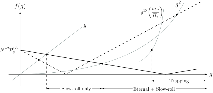
Figure 3: Intervals in the $g$-axis corresponding to the two inflationary regimes for $m_{\phi}^{2}\geq 0$. The function $f(g)$ features now a decreasing branch owing to $V_{0}^{\textrm{\tiny(3)}}$ and $m^{2}$ having different sign. If there is a growing branch, this may or may not intersect the curve $g^{2}$, depending on which term dominates $V(\phi)$ at $\bar{\phi}\sim\Phi_{\rm min}$. The ESP may be effectively considered as having $m_{\phi}^{2}\approx 0$ if the curve $g^{2}$ is intersected only once (bold line). Otherwise the mass term dominates the scalar potential and the field is temporarily stabilised at the minimum (dashed line).

If the quadratic term dominates at $\bar{\phi}\sim\Phi_{\rm min}$, the growing branch has two intersections with the curve $g^{2}$, allowing the regime with slow-roll only to be compatible with trapping for sufficiently large values of $m_{\phi}^{2}/H_{*}^{2}$. If the quadratic term is subdominant, the growing branch has no intersections with $g^{2}$, and the only intersection is in the decreasing branch. In this case, the limit $m_{\phi}^{2}\approx 0$ is recovered. These two possibilities are illustrated in Fig. 3.

Up to now, we have used a phase of slow-roll inflation to solve the flatness and horizon problems. However, it is also possible to solve these problems without slow-roll inflation, but with $|\eta|\sim 1$. The resulting phase of inflation is called fast roll inflation [37]. In our model, this possibility may arise if the ESP results in a maximum with $|m_{\phi}^{2}|\sim H_{*}^{2}$. From Eq. (30), the effective mass of the field is $m^{2}=m_{\phi}^{2}+V_{0}^{\textrm{\tiny(3)}}\bar{\phi}$. Therefore, $m^{2}$ remains within the order of $H_{*}^{2}$ for field displacements of $\bar{\phi}\lesssim m_{\phi}^{2}/V_{0}^{\textrm{\tiny(3)}}$. Fast-roll inflation then finishes at $\bar{\phi}_{\rm e}\sim m_{\phi}^{2}/V_{0}^{\textrm{\tiny(3)}}$, since for larger values $|m^{2}|>H_{*}^{2}$.

If the ESP results in a minimum where the field is temporarily stabilised. After tunneling the potential barrier, the field finds itself at distances of the order $m_{\phi}^{2}/|V_{0}^{\textrm{\tiny(3)}}|$. From that point onwards, enough inflation is only possible if $|\eta|<1$, which corresponds to slow-roll inflation. Fast-roll inflation is insufficient in this case.

Assuming then that the ESP results in a maximum, the equation of motion for $\phi$ may be approximated by

$$\ddot{\bar{\phi}}+3H\dot{\bar{\phi}}-|m_{\phi}^{2}|\bar{\phi}\simeq 0$$ (52)

for field values $\bar{\phi}\lesssim\bar{\phi}_{\rm e}$. This equation may then be solved [37], and the field value $N$ $e$-foldings before the end of fast-roll inflation given

$$\bar{\phi}\sim\bar{\phi}_{\rm e}\exp(-NF_{\phi})\,,$$ (53)

where $F_{\phi}$ is

$$F_{\phi}\equiv\frac{3}{2}\left(\sqrt{1+\frac{4}{3}|\eta|}-1\right)\,.$$ (54)

The amplitude of perturbation generated by the inflaton when the observable Universe leaves the horizon is ${\cal P}_{\phi}^{1/2}\sim H_{*}\delta\phi/\dot{\phi}$ [38]. Writing $N=H_{*}\Delta t$ we obtain $\dot{\phi}$ from Eq. (53), and taking $\delta\phi\sim H_{*}$ we have

$${\cal P}_{\phi}^{1/2}\sim\frac{H_{*}\exp(NF_{\phi})}{F_{\phi}}\frac{V_{0}^{\textrm{\tiny(3)}}}{m_{\phi}^{2}}\,.$$ (55)

Using the lower bound for $|V_{0}^{\textrm{\tiny(3)}}|$, Eq. (103), we obtain

$$\frac{H_{*}}{m_{P}}<\frac{|\eta|F_{\phi}}{\exp(NF_{\phi})}\frac{{\cal P}_{\phi}^{1/2}}{(c\sigma_{0})^{3}}\,,$$ (56)

thus constraining $H_{*}$ in terms of $|\eta|$. The bound is less stringent when the inflaton contributes significantly to the curvature perturbation, in which case

$$H_{*}<10^{6}\frac{|\eta|F_{\phi}}{\exp(NF_{\phi})}\,\,\textrm{TeV}\,,$$ (57)

where we take $c\sigma_{0}\sim 10$.

5 Quintessence

5.1 After the end of inflation

In the first stage of its evolution after inflation, the energy density of the field becomes again dominated by its kinetic energy because of the steepness of the scalar potential $V_{\rm np}$. This phase is known as kination, and the evolution of the field is governed by the equation

$$\ddot{\phi}+3H\dot{\phi}\simeq 0\,.$$ (58)

In order to achieve a successful model for quintessential inflation, the field cannot decay after the end of inflation, for otherwise it could not have survived until today to become quintessence. The usual assumption to get around this is to consider that the couplings of $\phi$ to the standard model particles are suppressed so that no instant preheating mechanism applies [29], thereby avoiding the decay of the field into a thermal bath of the standard model particles. This is reasonable to assume for a modulus field when away from ESPs.

To recover the Hot Big Bang (HBB) it is necessary to discuss an alternative method to achieve reheating after inflation. One possibility to do this is through the decay of a curvaton field [16]. As an additional advantage, this curvaton field helps to produce the correct amplitude of the primordial density perturbations [15], while it also allows more easily inflation to occur at relatively low energies [23, 24].

In this case, the phase of kination finishes when the curvaton, or its decay products, catches up with the kinetic energy of the field, eventually leading to the onset of the HBB. It is possible here to envisage two scenarios to end kination. One is to consider that the curvaton decays after the end of kination, and therefore a period of matter domination follows kination, during which the Universe is dominated by the oscillating curvaton field [16]. The other possibility is to consider that the curvaton field decays before kination finishes, and the Universe becomes radiation dominated at the end of kination. For our purposes these two cases are roughly equivalent, for, once kination finishes, the equation of motion of $\phi$ features an asymptotic value $\phi_{F}$, which does not differ much from one case to the other. Consequently we adopt the simplest scenario in which the curvaton field decays before it dominates, leading to radiation domination after kination. Therefore, at the end of kination the Hubble parameter is given by

$$H_{\rm rh}=\frac{\rho_{B}^{1/2}}{\sqrt{3}\,m_{P}}=\sqrt{\frac{\pi^{2}g_{\ast}}{90}}\frac{T_{\rm rh}^{2}}{m_{P}}\,,$$ (59)

where $g_{\ast}$ is the number of relativistic degrees of freedom, which for the Standard Model in the early Universe is $g_{\ast}=106.75$, and $T_{\rm rh}$ is the reheating temperature. Note that $T_{\rm rh}$ is not associated with the decay of the inflaton. It corresponds to the onset of the HBB.

It must be stressed here that the asymptotic value $\phi_{F}$ in the case of a double exponential potential is not finite due to the steepness of the potential. However, $\phi_{F}$ is finite if $V(\phi)$ takes the form of the typical exponential-like uplifting potential

$$V(\phi)\simeq C_{n}e^{-b\phi/m_{P}}\,,\quad\textrm{or}\quad V(\sigma)\simeq C_{n}\sigma^{-n}\,,$$ (60)

in terms of $\sigma$ (see Eq. (29)), where $C_{n}$ is a density scale and

$$b=\sqrt{2/3}\,n\,.$$ (61)

Since its introduction in Ref. [40] to help stabilise the volume modulus of type IIB compactifications in de Sitter vacua, this kind of exponential-like potential has become widespread as uplifting term. However, in our model such an uplifting term does not stabilise the field in a minimum of the potential. Instead, the uplifting term, when it dominates over non-perturbative contributions at large field values, allows the field to freeze temporarily due to excessive cosmic friction. This excess of cosmic friction may be invoked as well when the uplifting term cooperates with some non-perturbative contribution to produce a minimum in the scalar potential, thus assisting moduli stabilisation as in Ref. [41].

5.2 Coincidence and constraints from BBN

Once the field reaches its value $\phi_{F}$, it remains frozen until the density of the Universe is comparable to $V(\phi_{F})$. Hence, in order for the field $\phi$ to become quintessence, we have to constrain its evolution with the so-called coincidence requirement. This requires that the value at which the field freezes, $\phi_{\rm F}$, at the beginning of the HBB is such that

$$V(\phi_{\rm F})\simeq\Omega_{\phi}\rho_{0}\,,$$ (62)

where $\Omega_{\phi}\sim 0.7$ is the ratio of the scalar density to the critical density, and $\rho_{0}$ denotes the energy density of the Universe today.

The subsequent evolution of the field depends strongly on the value of the slope $b$ in Eq. (60) [9, 10]. If $b^{2}<2$ the potential density of the scalar field becomes dominant, and the Universe engages in a phase of eternal acceleration. Even though string theory disfavors this possibility due to the appearance of future horizons [42], this scenario cannot be ruled out from observations. It is possible as well that the scalar density becomes dominant without causing eternal acceleration. This occurs for slopes in the interval $2<b^{2}<3(1+w_{B})$, where $w_{B}$ is the barotropic parameter for the background component.

If the slope of the potential lies in the interval $3(1+w_{B})<b^{2}<\sqrt{6}$, then the field unfreezes following an attractor that mimics the background component. This solution has $\rho_{\phi}/\rho_{B}=\textrm{const.}<1$ [9]. However, the field does not follow this attractor immediately. It has been shown [43] that the field oscillates for some time around its attractor solution before it starts to follow its attractor. Numerical computations [44] show that a short period of accelerated expansion is possible, even in the case of dark energy domination without eternal acceleration. In fact, this acceleration is found when the slope $b$ in Eq. (60) lies in the interval

$$2\lesssim b^{2}\lesssim 24\,,$$ (63)

which is equivalent to $\sqrt{3}\leq n\leq 6$. More recent studies have reduced this range somewhat. According to Ref. [45] accelerated expansion is possible only if $b^{2}<27/8$. This would mean that brief acceleration is possible in the range $\sqrt{3}\leq n<9/4$. However, the observational constraints on the density parameter and the equation of state of Dark Energy are heavily dependent on priors (such as a assuming a cosmological constant for the former or primordial curvature perturbations with a constant spectral index for the latter) as also acknowledged in Ref. [45]. This means that, were those priors modified or removed, the allowed range of $n$ may be well enlarged. In Sec. 6 we comment on how an exponential potential with slope $b$ in the above interval can be theoretically motivated. Now we describe how the coincidence requirement constrains our system once we consider the term in Eq. (60) as the dominant contribution to the scalar potential.

As we said before, after the end of inflation the scalar field is governed by Eq. (58) with $H=1/3t$, thus growing with time as $\sim\ln t$. However, once the Universe becomes radiation dominated, with $H=1/2t$, the equation of motion features an asymptotic value for $t\to\infty$ [9, 10]. This value $\phi_{F}$ is given by

$$\phi_{F}\sim\phi_{\rm e}+\sqrt{\frac{2}{3}}\,m_{P}\,\textrm{ln}\left[\sqrt{\frac{90}{\pi^{2}g_{\ast}}}\frac{H_{*}\,m_{P}}{T_{\rm rh}^{2}}\right]=\phi_{\rm e}+\Delta\phi_{F}\,,$$ (64)

We note here that at the end of inflation the field is very close to the ESP, i.e. $\bar{\phi}_{\rm e}<m_{P}$, whereas $\Delta\phi_{\rm F}>m_{P}$. Assuming also that $\phi_{0}\lesssim m_{P}$, we approximate $\phi_{F}\approx\Delta\phi_{\rm F}$, with the corresponding field $\sigma_{F}$ given by

$$\sigma_{F}\sim\left[\sqrt{\frac{90}{\pi^{2}g_{\ast}}}\frac{H_{*}\,m_{P}}{T_{\rm rh}^{2}}\right]^{2/3}\,.$$ (65)

Hence, given that the field has to cover a number of Planck lengths to reach the value $\phi_{F}$, the non-perturbative potential $V_{\rm np}(\phi)$ becomes subdominant with respect to the uplift potential in Eq. (60). Assuming that this is the case at $\phi\sim\phi_{F}$, Eq. (62) applied to such a potential allows us to estimate the reheating temperature

$$T_{\rm rh}\sim\sqrt{H_{*}\,m_{P}}\left(\frac{\rho_{0}}{C_{n}}\right)^{\sqrt{3/8n^{2}}}\,.$$ (66)

Requiring now the reheating temperature to be larger than the temperature at Big Bang Nucleosynthesis (BBN), $T_{\rm BBN}$, we obtain the bound

$$C_{n}\lesssim\rho_{0}\left(\frac{\sqrt{H_{*}\,m_{P}}}{T_{\rm BBN}}\right)^{2n\sqrt{2/3}}\,.$$ (67)

5.3 Constraints from gravitational waves

Now we look at the constraints imposed by the density of gravitons produced during the inflationary process. Models of quintessential inflation are known to have a relic graviton spectrum with three different regions. This is the result of the intermediate phase of kination between the inflationary expansion and the HBB. Due to the stiff equation of state during kination, the spectrum exhibits a spike that corresponds to the production of gravitons at high frequencies [46].

Due to the presence of the spike at high frequencies, it is necessary to impose an integrated bound in order not to disturb BBN predictions. The constraint is [10]

$$I\equiv h^{2}\int_{k_{\rm BBN}}^{k_{e}}\Omega_{\rm GW}(k)\,d\ln k\leq 2\times 10^{-6}\,,$$ (68)

where $\Omega_{\rm GW}(k)$ is the density fraction of the gravitational waves (GWs) with physical momentum $k$, $h=0.73$ is the Hubble constant $H_{0}$ in units of $100$ km/sec/Mpc. Using the spectrum $\Omega_{\rm GW}(k)$ as computed in Ref. [46], the constrain above can be written as [10]

$$I\simeq h^{2}\alpha_{\rm GW}\Omega_{\gamma}(k_{0})\frac{1}{\pi^{3}}\frac{H_{*}^{2}}{m_{P}^{2}}\left(\frac{H_{*}}{H_{\rm rh}}\right)^{2/3}\,,$$ (69)

where $\alpha_{\rm GW}\simeq 0.1$ is the GW generation efficiency during inflation, $\Omega_{\gamma}(k_{0})=2.6\times 10^{-5}h^{-2}$ is the density fraction of radiation at present on horizon scales, and “rh” denotes the end of kination. Making use of Eq. (59) the bound above becomes

$$I\simeq\frac{\alpha_{\rm GW}\Omega_{\gamma}(k_{0})}{3\pi^{3}}\left(\frac{30}{\pi^{2}g_{\ast}}\right)^{1/3}\frac{3H_{*}^{2}}{m_{P}^{2}}\left(\frac{H_{*}m_{P}}{T_{\rm rh}^{2}}\right)^{2/3}\,.$$ (70)

Substituting the values given above, and applying the bound in Eq. (68) we obtain

$$\frac{3H_{*}^{2}}{m_{P}^{2}}\left(\frac{H_{*}m_{P}}{T_{\rm rh}^{2}}\right)^{2/3}\lesssim 4\times 10^{2}\,.$$ (71)

Using the minimum reheating temperature $T_{\rm rh}\sim T_{\rm BBN}\sim 1$ MeV we find the constraint

$$H_{*}\lesssim 10(m_{P}T_{\rm BBN})^{1/2}\sim 10^{5}\,\textrm{TeV}\,,$$ (72)

whereas for larger reheating temperature the corresponding bound is less demanding.

6 Quintessence in Flux Compactifications

In this section we discuss whether it is possible to realise our model of quintessential inflation with the volume modulus of type IIB string theory. Such a realisation posseses a number of well-known problems. One of them is related to the variation of fundamental constants in nature. This problem can be overcome since in the later part of the Universe history the field is frozen, and starts evolving only today with a characteristic time of variation within the order of the Hubble time. This fact makes quintessence consistent with no variation in the fundamental constants.

Another problem is that moduli fields couple to ordinary matter with gravitational strength, therefore giving rise to long-range forces, which are strongly constrained by observations. A possible way out is to consider that the coupling of the inflaton-quintessence modulus to baryonic matter is further suppressed.

We discuss now a number of possible origins for the exponential term $C_{n}\sigma^{-n}$ realising the quintessential part of the evolution. In this paper we consider a string modulus field as quintessence. The scalar potential of such a field is flat to all orders in perturbation theory. Hence, a modulus field obtains its mass solely through non-perturbative effects. Along with these non-perturbative effects, there is a number of possible contributions that one may consider. In type IIB compactifications, the non-perturbative contributions to the scalar potential $V(\phi)$ depend on the volume of the compactified space, parametrised by the volume modulus $T$. The realization of quintessence with this volume modulus $T$ considers the stabilisation of the volume of the internal manifold due to excessive cosmic friction [10, 14], rather than the stabilisation at a minimum of the scalar potential. This, in turn, puts forward the possibility of having a dynamical internal manifold rather than a frozen one, as has been recently suggested in the literature [47].

It must be stressed that the crucial event in this stabilisation setting is the reheating of the Universe achieved through the decay of a curvaton field. The decay products of such curvaton field provides a thermal bath that sources the cosmic friction which freezes the field, as explained in Sec. 5.

6.1 Through non-perturbative effects

In type IIB compactifications, certain combinations of fluxes can stabilise the dilaton and complex structure moduli [33]. The warp factor for antibranes can be computed in terms of these fluxes, and it is found that this is minimized if the antibrane is located at the tip of the Klebanov-Strassler throat. For a set of $N$ branes sitting at the tip of the throat the warp factor is [33]

$$e^{A_{\rm min}}\sim e^{-2\pi K/3Mg_{s}}\,,$$ (73)

where $g_{s}$ is the string coupling. The $\overline{D3}$-brane introduces an uplifting term in the scalar potential which, written in Planck units, is given by

$$\delta V(\sigma)\sim\frac{e^{4A_{\rm min}}}{\sigma^{2}}\equiv C_{2}\sigma^{-2}\,.$$ (74)

This contribution dominates the scalar potential for large values of $\sigma$ where the non-perturbative potential $V_{\rm np}$, due to its steepness, is subdominant. Consequently, at large values of $\sigma$ we approximate the scalar potential as $V(\phi)\simeq\delta V$.

The reliability of the supergravity approximation in this context requires $g_{s}M>1$ [48]. Also, to obtain $C_{2}$ small enough to comply with the coincidence requirement embodied in Eq. (67), we must consider a choice of fluxes such that

$$K>g_{s}M>1\,.$$ (75)

Tuning appropriately these values we can always generate the appropriate scale for $C_{2}$. Also, in view of Eq. (66), this allows us to increase the reheating temperature at the onset of the HBB by increasing the units of flux K.

In this case $n=2$. Then, taking for example $H_{*}\sim 1\,$TeV, $T_{\rm BBN}\sim 10\,$MeV and $\rho_{0}\sim 10^{-120}\,m_{P}^{4}$, Eq. (67) gives

$$C_{2}^{1/4}\lesssim 10^{-20}m_{P}\,.$$ (76)

In this case, the ratio between fluxes must be $K/Mg_{s}\gtrsim 22$. Taking $g_{s}=0.1$, only approximately twice as many units of $K$ flux as those of $M$ flux are needed to generate the appropriate energy scale.

It is also possible to consider other sources for the uplifting term $\delta V$, like for example the introduction of fluxes of gauge field on $D7$-branes [49]. In this case, the scalar potential $V(\phi)$ is modified in a similar way, obtaining now

$$\delta V\sim\frac{2\pi E^{2}}{\sigma^{3}}\equiv C_{3}\sigma^{-3}\,,$$ (77)

where $E$ depends on the strength of the gauge fields considered.

In this case the constraint on $C_{3}$ is alleviated thanks to the higher value of $n$. If we consider $H_{*}\sim 1$ TeV as before, then Eq. (67) gives now

$$C_{3}^{1/4}\lesssim 10^{-15}m_{P}\,,$$ (78)

which corresponds to an energy scale roughly within the order of the TeV.

6.2 In string perturbation theory

Another kind of corrections introducing an uplifting term in the scalar potential $V(\phi)$, changing its structure at large volume and breaking the no-scale structure, are $\alpha^{\prime}$ corrections [50].

We consider the simplest case in which the volume of the compactified space is determined by one single volume modulus $T$. In this case, the volume of the internal manifold in the Einstein frame is ${\cal V}=(T+\bar{T})^{3/2}$. This case has already been considered in the literature [51]. The corrected Khäler potential is

$$K=K_{0}-2\textrm{ln}\left(1+\frac{\hat{\xi}}{2(2\textrm{Re}\,T)^{3/2}}\right)\,,$$ (79)

where $K_{0}=-3\textrm{ln}\,(T+\bar{T})$ is the tree-level Khäler potential, and $\hat{\xi}=-\frac{1}{2}\zeta(3)\chi e^{-3\varphi/2}$ where $\chi$ is the Eüler number of the internal manifold, and $e^{\varphi}=g_{s}$ is the string coupling. We consider the superpotential with only one non-perturbative contribution $W=W_{0}+Ae^{-c\sigma}$. For large values of $\sigma=\textrm{Re}\,T$ we can approximate the superpotential by the classical one $W=W_{0}$. In this case, the scalar potential computed from $W=W_{0}$ using the Kähler potential in Eq. (79) is

$$V\approx\delta V\sim\frac{\hat{\xi}\,W_{0}^{2}}{(\textrm{Re}\,T)^{9/2}}\,,$$ (80)

for the tree level potential is exponentially suppressed for large values of $\sigma$ [c.f. Eq. (27)]. When $(\textrm{Re}\,T)^{3/2}$ is large compared to $\hat{\xi}$ we can compute the canonically normalized field $\phi$ using $K\approx K_{0}$. As a result, $\phi$ is still given by Eq. (29), and consequently we can identify the exponential potential in terms of $\sigma$

$$\delta V\sim\frac{\hat{\xi}\,W_{0}^{2}}{\sigma^{9/2}}\equiv C_{9/2}\sigma^{-9/2}\,.$$ (81)

In this case, the bound for $C_{9/2}$ obtained using Eq. (67) with $H_{*}\sim 1$ TeV results in

$$(C_{9/2})^{1/4}\lesssim 10^{-7}m_{P}\,,$$ (82)

where the upper bound corresponds to the intermediate scale $C_{9/2}^{1/4}\sim 10^{11}$ GeV.

6.3 Constraints on the volume modulus

Not only must this picture be consistent from the theoretical point of view, but also from the observational one. In this sense, it is well known that the excessive production of light moduli fields with a late decay can spoil the abundance of light elements predicted by BBN. Here, we are interested in the risks put forward by the volume modulus. The most evident one is that, given that this field controls the volume of the compactified space, Kaluza-Klein modes may jeopardize BBN predictions.

In closed string theory, in addition to the usual translational modes, vibrational modes of closed strings wrapping around the compact manifold are also present. The mass of these excitations follows an inverse relation to the radius of the compactification [52]

$$m_{\rm KK}\sim\frac{m_{s}}{R}\sim\frac{g_{s}\,m_{P}}{{\cal V}^{2/3}_{\rm st}}\,,$$ (83)

where $R$ is the radius of the compactified space defined by the volume of the Calabi-Yau manifold ${\cal V}_{\rm st}\sim R^{6}$, $g_{s}$ is the string coupling and $m_{s}$ the string mass scale.

We now constrain the volume of the compactified space in order to avoid a late decay disturbing the abundances of light elements predicted by BBN. Recalling now Eq. (65) for the frozen field, we can estimate the volume ${\cal V}_{\rm st}(\sigma_{F})$, with which we can compute the mass of the lightest KK modes, as given by Eq. (83). Also, assuming interaction of at least gravitational strength, these modes decay at the temperature

$$T_{\rm KK}\sim\sqrt{\Gamma\,m_{P}}\sim\frac{g_{s}^{3/2}m_{P}}{\sigma_{F}^{3/2}}\,,$$ (84)

where we have considered the decay rate $\Gamma\sim m_{\rm KK}^{3}/m_{P}^{2}$. In order to preserve the abundances predicted by BBN we require $T_{\rm KK}>T_{\rm BBN}$. The frozen field value $\sigma_{F}$ is thus forced to satisfy

$$\sigma_{F}<\left(\frac{g_{s}^{3/2}m_{P}}{T_{\rm BBN}}\right)^{2/3}\,.$$ (85)

Applying this bound to the expression in Eq. (65) for the frozen field results in a bound for the reheating temperature $T_{\rm rh}$

$$T_{\rm rh}>\left[\frac{30}{\pi^{2}g_{\ast}g_{s}^{3}}\right]^{1/4}\sqrt{T_{\rm BBN}\,H_{*}}\sim\sqrt{T_{\rm BBN}\,H_{*}}\,,$$ (86)

which for $H_{*}\sim\,1\,\textrm{TeV}$ and $T_{\rm BBN}\sim\,1$ MeV results in $T_{\rm rh}>1$ GeV. Taking then the reheating temperature $T_{\rm rh}\sim\,10$ GeV alleviates the constraint on $H_{*}$ imposed by Eq. (71), which now becomes

$$H_{*}\lesssim 10^{7}\,\textrm{TeV}\,.$$ (87)

However, the reheating temperature results in a significantly stronger bound on the coefficient $C_{9/2}$. Using Eq. (66) with $T_{\rm rh}\sim 10$ GeV we obtain

$$C_{9/2}^{1/4}\lesssim 10^{-12}m_{P}\sim 10^{6}\textrm{ GeV}\,.$$ (88)

7 Summary and Conclusions

We have investigated in detail a realisation of quintessential inflation within the framework of string theory. Our inflaton - quintessence field is a string modulus with a characteristic runaway scalar potential. In our treatment we have avoided to specify in full detail our string inspired theoretical basis in order for our considerations to remain as generic as possible. In that sense, our quintessential inflation realisation is more like a paradigm than a specific model.

In this spirit we considered a broadly accepted form of the non-perturbative superpotential (which can be due to, for example, gaugino condensation or $D$-brane instantons) and of the tree-level Kähler potential shown in Eqs. (24) and (26) respectively. The resulting non-perturbative potential appears in Eq. (27) and is of the form $V_{\rm np}(\sigma)\propto\sigma^{-\ell}e^{-\mu c\sigma}$, where $\sigma=$ Re $T$ and $\ell,\mu=1,2$ depending which term dominates. Due to Eq. (26) the canonically normalised modulus $\phi$ is in fact related to $\sigma$ as $\sigma(\phi)=e^{\sqrt{\frac{2}{3}}\phi/m_{P}}$ [c.f. Eq. (29)]. Hence, the potential $V_{\rm np}(\phi)$ is, in fact, of the form of a double exponential.

Such a potential is too steep to support inflation. This is why, we have assumed the existence of an enhanced symmetry point (ESP) at some value $\phi_{0}$, corresponding to potential density $V_{0}=3H_{*}^{2}m_{P}^{2}$. The most salient effect of the ESP is that it can trap the rolling modulus and effectively stop it from rolling. Indeed, as the modulus crosses the ESP, particle production can generate a contribution $V_{\rm int}(\phi)$ to the scalar potential able to stop the roll of the modulus and trap the latter at the ESP. However, apart from the phenomenon of particle production described in [12], in this paper we have also taken into account that the ESP generates a ‘flat patch’ on the scalar potential because of the condition $V^{\prime}(\phi_{0})=0$. Hence, all things considered, the trapping mechanism that operates at the ESP may set the field at a locally flat region in field space. In this paper we show how, after the field is released from its trapping, this flatness may result in enough inflation to solve the flatness and horizon problems.

After being trapped, the modulus oscillates around the ESP under the influence of $V_{\rm int}(\phi)$. These oscillations deplete its initial kinetic density until the latter decreases below $V_{0}$, in which case a phase of so-called trapped inflation begins [12]. Trapped inflation dilutes $V_{\rm int}$ until the latter is unable to restrain the field, at which time the modulus is released and continues rolling over $V(\phi)$. As we have shown, trapped inflation is brief and cannot suffice for the solution of the horizon and flatness problems. The duration of trapped inflation is independent from the value of the initial kinetic density of the modulus, because all excess of the latter is depleted before the onset of trapped inflation. Hence, our framework is largely independent of initial conditions, provided trapping occurs.

To study the dynamics after the field is released from its trapping, we have followed a phenomenological approach. In it, the scalar potential $V(\sigma)$ consists of a ‘background’ potential $V_{\rm np}(\sigma)$ of non-perturbative origin (from gaugino condensation, for example), and a phenomenological potential $V_{\rm ph}(\sigma)$ chosen so that the scalar potential $V(\sigma)=V_{\rm np}(\sigma)+V_{\rm ph}(\sigma)$ satisfies $V^{\prime}(\phi_{0})=0$. The guiding line to pick out $V_{\rm ph}$ is to demand that it decreases faster than $V_{\rm np}$, so that the former is only important when the field is close to the ESP. Given the characteristic form of $V_{\rm np}(\sigma)$, the simplest choice for $V_{\rm ph}$ is to take $V_{\rm ph}\propto e^{-q\sigma}$ far from the ESP with $q>\mu c$ a constant. A particular realisation of $V_{\rm ph}$ is given in Eq. (95). In this setting, we show in Appendix 9.2 that the terms of order forth and higher in a series expansion around the ESP become important only after the end of inflation. Therefore, the inflationary dynamics can be fully accounted for through the scalar potential $V(\phi)=V_{0}+\frac{1}{2}m_{\phi}^{2}\bar{\phi}^{2}+\frac{1}{3!}V_{0}^{\textrm{\tiny(3)}}\bar{\phi}^{3}$, where $\bar{\phi}\equiv\phi-\phi_{0}$.

In this paper we are concerned with the observable amount of inflation. We thus pay special attention to the last $N\approx 60$ $e$-foldings of inflation, and compute the curvature perturbation, ${\cal P}_{\phi}^{1/2}$, generated by the inflaton field when the observable Universe leaves the horizon. We show how in our model $V_{0}^{\textrm{\tiny(3)}}$ is fully determined by $H_{*}$ and ${\cal P}^{1/2}_{\phi}$, Eq. (40). This offers two significant advantages. First, the dynamics becomes described in terms of simple and meaningful physical quantities relevant to inflation. Second, the parameter space of the model becomes automatically constrained by the observed value of the curvature perturbation, which ${\cal P}_{\phi}^{1/2}$ cannot exceed, i.e. ${\cal P}_{\phi}^{1/2}\lesssim 4.8\times 10^{-5}$. Note that the observed curvature perturbation in our model is generated by a curvaton field which is also employed to reheat the Universe.

A side effect of our model is that it imposes a lower bound in ${\cal P}_{\phi}^{1/2}$ [c.f. Eq. (41)], which in turn translates into an upper bound on $H_{*}$, Eq. (42). We recognise these bounds as an artifact of the model, that appears when we parametrise our ignorance about the behaviour of $V(\phi)$ around the ESP. A simple way around these unphysical bounds is to let $q$ have a running.

We find that we can attain enough inflation to solve the flatness and horizon problems if $|m_{\phi}|\lesssim H_{*}$ and $V_{0}^{\textrm{\tiny(3)}}\ll H_{*}$. In particular, we discover that the field may have two different inflationary histories, or regimes, ending in a phase of slow-roll during which the observable Universe leaves the horizon. Whereas one of the inflationary regimes consists only of slow-roll inflation, the other regime involves a previous phase of eternal inflation. Eqs. (36) and (37) [c.f. Eq. (33)] determine which of these inflationary regimes will be driven by the field. Of course, consistency requires that the regimes must be compatible with the trapping condition, Eq. (44). The values of $g$ corresponding to the different inflationary regimes, and to the trapping condition, are pictured in Figs. 2 and 3, corresponding to $m_{\phi}^{2}<0$ and $m_{\phi}^{2}\geq 0$ respectively. The results in both cases are qualitatively the same: the inflationary regime involving eternal inflation is always compatible with trapping. However, the inflationary regime where only slow-roll inflation occurs, is compatible with trapping only if $|\eta|$ when sufficiently large, Eq. (48). Finally, an acceptable inflationary cosmology is also achievable through fast-roll inflation. This possibility arises only when the ESP results in a maximum with $|m_{\phi}^{2}|\sim H_{*}^{2}$. In this case, $H_{*}$ must satisfy an upper bound, Eq. (56), so that the field does not generate an excessive amount of perturbations.

After inflation is terminated the field becomes dominated by its kinetic density and the Universe enters a period of so-called kination [13]. During this period the modulus is oblivious of the scalar potential and its rapid roll can send it very far in field space. To reheat the Universe we have assumed a curvaton field, whose decay products in time dominate the kinetic density of the rolling modulus [16]. The existence of a suitable curvaton, apart from reheating the Universe, can also provide the required density perturbations [15] and allow for a low inflation scale [21, 24]. After reheating, the modulus roll is inhibited by cosmological friction as discussed in Refs. [10, 14]. Consequently, in little time, the modulus freezes at a value $\sigma_{F}$ shown in Eq. (65). The modulus remains frozen until the present, which guarantees the non-variation of the fundamental constants through-out the hot big bang despite the fact that the modulus is not stabilised in a local minimum. Eq. (65) shows that $\sigma_{F}$ depends on the reheating temperature, which, in turn, depends on the details of the curvaton model. Therefore, in our framework curvaton physics can determine the value of the string modulus in our Universe.

After the end of kination the modulus is expected to freeze at a large value at the tail of the scalar potential. At such values, we assume that the latter may be dominated by a contribution of the form $V(\sigma)=C_{n}/\sigma^{n}$ [c.f. Eq. (60)], where $C_{n}$ is a density scale and the value of $n$ is model dependent. The value of $C_{n}$ is determined by the coincidence requirement, if the modulus is to become quintessence at present. This requirement results in the constraint in Eq. (66), where we see that $C_{n}$ depends also on the reheating temperature and, therefore, it is determined by curvaton physics. The requirement that reheating occurs before Big Bang Nucleosynthesis (BBN) sets an upper bound on $C_{n}$, shown in Eq. (67). Crucially, the bound is strongly $n$-dependent.

This type of uplifting potential is again broadly accepted in string flux compactifications.We have discussed some possibilities for the origin of the uplifting potential, such as RR and NS fluxes on $\overline{D3}$-branes (where $n=2$ and $C_{2}^{1/4}\lesssim 10$ MeV), gauge field fluxes on $D7$-branes (where $n=3$ and $C_{3}^{1/4}\lesssim 1$ TeV) and $\alpha^{\prime}$-corrections (where $n=9/2$ and $C_{9/2}^{1/4}\lesssim 10^{11}$ GeV). $C_{n}$ may be further constrained in order to protect BBN from heavy KK modes. It turns out that this constraint is important only in the $n=9/2$ case where the bound on $C_{9/2}$ is strengthened to $C_{9/2}^{1/4}\lesssim 10^{6}$ GeV. Note that the above bounds are much more reasonable than the fine-tuning of $\Lambda$ required in $\Lambda$CDM.

According to Eq. (60), the scalar potential for the canonically normalised field $\phi$ is of exponential form. For the above discussed values of $n$ and according to Ref. [44] the modulus can cause a brief period of accelerating expansion while it unfreezes at present [9]. Thus, our model does not lead to eternal acceleration and therefore does not suffer from the existence of future horizons [42]. In the future, the modulus eventually approaches $+\infty$ which corresponds to a supersymmetric ground state. If $\sigma$ is the volume modulus then this final state leads to decompactification of the extra dimensions.

Some numerical simulations more recent than Ref. [44] suggest that the parameter space for brief acceleration is somewhat reduced. In particular, in Ref. [53] the authors demonstrate that brief acceleration can indeed take place in the interval $\sqrt{2}<b\leq\sqrt{3}$ corresponding to the range $\sqrt{3}<n\leq 3/\sqrt{2}$, which includes the case $n=2$. This is confirmed by Refs. [54] and [55], where it is implied that brief acceleration, which is terminated at present, can be attained even for larger values of $b$. In Ref. [45] it is indeed shown that one may have brief acceleration up to the value $b=\frac{3}{4}\sqrt{6}$ corresponding to $n=9/4$. The authors of Ref. [45] acknowledge the fact that the parameter space determined by observations is affected by assumed priors and may be extended further. Hence, the case $n=3$ might still be successful. However, in view of the above, the case of $\alpha^{\prime}$-corrections to the Kähler potential (Sec. 6.2) is probably excluded.

In conclusion, we have investigated a paradigm of quintessential inflation using a sting modulus as the inflaton - quintessence field. We have shown that there exists ample parameter space for successful quintessential inflation to occur with reasonable values of the model parameters (with possibly a mild tuning of gravitational couplings between the modulus and the standard model fields, required to overcome the 5th force problem). The possibility of attaining an acceptable inflationary cosmology depends crucially on the values of $V_{0}^{\textrm{\tiny(3)}}$ and $m_{\phi}$ relative to the Hubble scale $H_{*}$ during inflation. The latter is determined by the location of the ESP and can be much different to $m_{\phi}$ or $V_{0}^{\textrm{\tiny(3)}}$. Furthermore, a crucial role is played by the value of the reheating temperature, which controls both the value of the frozen modulus and the required value of the density scale in the uplift potential. The reheating temperature is determined, in turn, by the particulars of the assumed curvaton field. Because the modulus remains frozen until the present, the model may conceivably be linked to the intriguing possibility that some of the fundamental constants, such as the fine-structure constant, may begin to vary at present.

8 Acknowledgments

We wish to thank James Gray for useful comments and Lorenzo Sorbo for stimulating discussions. KD wishes to thank Steve Giddings and Marios Petropoulos for interesting discussions and the Aspen Center for Physics for the hospitality. This work was supported (in part) by the European Union through the Marie Curie Research and Training Network ”UniverseNet” (MRTN-CT-2006-035863) and by PPARC (PP/D000394/1). KD is supported by PPARC grant PPA/Y/S/2002/00272 and EU grant MRTN-CT-2004-503369.

9 Appendix

9.1 Elucidating the oscillatory regime

The key point to solve the oscillatory regime is to determine how the mass term $g^{2}\phi^{2}$ decreases in relation to the kinetic term $k^{2}$ (see Eq. (7)) once particle production finishes.

After the field crosses the ESP for the first time, the occupation number becomes $n_{k}^{(1)}=\exp(-\pi k^{2}/g\dot{\phi}_{0})$. During particle production we assume the same growth of the occupation number in all of the excited $\chi$ modes every time the field crosses the ESP. In this case, the occupation number at the end of particle production becomes $n_{k}^{\rm end}\sim g^{-2}\exp(-\pi k^{2}/g\dot{\phi}_{0})$.

In this process of particle production the expansion of the Universe is neglected. Therefore, if we consider the expansion of the Universe after particle production, the occupation number for a $\chi$-mode with physical momentum $k$ becomes

$$n_{k}^{\rm end}\sim g^{-2}\exp(-\pi(ka)^{2}/g\dot{\phi}_{0})\,.$$ (89)

Let us now consider $a\simeq 1$. Given that $m^{2}\gg H^{2}$ at the end of particle production, we can approximate the integral

$$\langle\chi^{2}\rangle\propto\int_{0}^{\infty}\frac{n_{k}^{\rm end}k^{2}dk}{\sqrt{k^{2}+g^{2}\phi^{2}}}$$ (90)

by replacing the field $\phi$ by its average $\overline{\phi}(t)\approx\Phi(t)$. Now, the main contribution to the average expectation value $\langle\overline{\chi^{2}}\rangle$ for $a\simeq 1$, comes from momenta $k^{2}\sim(g\dot{\phi}_{0})\sim g^{2}\Phi^{2}$. Therefore, we can approximate the integral by absorbing the term $g^{2}\Phi^{2}$ into $k^{2}$, namely $k^{2}+g^{2}\Phi^{2}\approx 2k^{2}\sim k^{2}$, thus obtaining

$$\langle\overline{\chi^{2}}(t)\rangle\sim g^{-2}\int_{0}^{\infty}\textrm{exp}(-\pi(ka)^{2}/g\dot{\phi}_{0})\,k\,dk\propto a^{-2}\,.$$ (91)

On the other hand, given that the $\chi$ particles become relativistic at the end of particle production, their average density $\overline{\rho}_{\chi}\sim n_{\chi}\sqrt{k^{2}+g^{2}\Phi^{2}}$ must scale as $a^{-4}$. We thus conclude that $\Phi$ must initially scale at least as fast as $a^{-1}$, for otherwise the mass term $g^{2}\Phi^{2}$ would dominate over $k^{2}$ in the average density $\overline{\rho}_{\chi}$.

To compute the initial scaling law for $\Phi$ we compute the depletion rate of the modulus density in the time-dependent quadratic potential $V_{\rm int}(\phi,\chi)=\frac{1}{2}g^{2}\langle\chi^{2}\rangle\phi^{2}$. Owing to $m^{2}>H^{2}$, the depletion rate of the energy of the oscillations $\rho_{\rm osc}$ can be computed following Ref. [56]. We find

$$\rho_{\rm osc}\propto a^{-4}\,.$$ (92)

Writing now $\rho_{\rm osc}=V_{\rm int}(\Phi)\propto a^{-2}\Phi^{2}$ we conclude that

$$\Phi\propto a^{-1}\,.$$ (93)

This result is valid just for $a\simeq 1$. However, this scaling for $\Phi$ implies that $\langle\chi^{2}\rangle$ remains independent of $\phi$, which in turn prevents $\Phi$ from decreasing faster than $a^{-1}$. If $\Phi$ decreased slower than $a^{-1}$, then the term $g^{2}\Phi^{2}$ would come to dominate $k^{2}$. In this case we have $\langle\chi^{2}\rangle\propto n_{\chi}\phi^{-1}$, and again a time-dependent linear potential in $\phi$: $V_{\rm int}\propto n_{\chi}\phi$. Following Ref. [56], we obtain that the amplitude $\Phi$ in this case scales exactly as before, i.e. $\Phi\propto a^{-1}$.

We conclude that as soon as particle production finishes, the amplitude of oscillations $\Phi$ and the expectation value $\langle\overline{\chi^{2}}\rangle$ scale as follows

$$\Phi\propto a^{-1}\quad\textrm{and}\quad\langle\overline{\chi^{2}}\rangle\propto a^{-2}\,,$$ (94)

and the regime is maintained as long as $m^{2}>H^{2}$.

9.2 Minimal realisation of an ESP

Our minimal realisation is based on the condition that the phenomenological term $V_{\rm ph}$ becomes subdominant with respect to the non-perturbative contribution $V_{\rm np}\propto\sigma^{-\ell}e^{-\mu c\sigma}$ when the field is away from the symmetry point. This means that $V_{\rm ph}$ must at least decrease exponentially when it starts to become subdominant. A particular choice to fulfill this is

$$V_{\rm ph}(\sigma)=-\frac{M_{\rm ph}}{\cosh^{-q}(\sigma-\Sigma)}\,,$$ (95)

which results in the scalar potential

$$V(\sigma)\approx M_{\rm np}\sigma^{-\ell}e^{-\mu c\sigma}-M_{\rm ph}\cosh^{-q}(\sigma-\Sigma)\,.$$ (96)

To account now for an ESP we impose

$$\frac{\partial V}{\partial\sigma}\Big{|}_{\sigma_{0}}=0\quad\textrm{and}\quad\frac{\partial^{2}V}{\partial\sigma^{2}}\Big{|}_{\sigma_{0}}=\frac{3}{2}\frac{m_{\phi}^{2}}{\sigma_{0}^{2}}\,,$$ (97)

where $m_{\phi}^{2}=V^{\prime\prime}_{0}$. To have a positive density at the ESP while satisfying Eqs. (97), we must impose $\sqrt{q}>\mu c$ (typical values are $c\lesssim 1$, so one may take $q\gtrsim 1$). We then describe the parameter space of the model through the variable

$$\xi\equiv\frac{\sqrt{q}}{c\mu}>1\,.$$ (98)

This quantity determines how close to the ESP the potential $V_{\rm ph}(\sigma)$ becomes exponentially suppressed with respect to $V_{\rm np}(\sigma)$. The scaling of these two contributions with $\sigma$ may be estimated as

$$V_{\rm np}(\sigma)\propto e^{-\mu c\bar{\sigma}}\left(\frac{\sigma_{0}}{\sigma}\right)^{\ell}\quad,\quad V_{\rm ph}(\sigma)\propto e^{-q\bar{\sigma}}\,.$$ (99)

where $\bar{\sigma}\equiv\sigma-\sigma_{0}$. Therefore, writing $r\equiv V_{\rm ph}(\sigma)/V_{\rm np}(\sigma)$, we have

$$\frac{r(\sigma)}{r(\sigma_{0})}\sim\left(1+\frac{\bar{\sigma}}{\sigma_{0}}\right)^{\ell}\displaystyle e^{-(q-\mu c)\bar{\sigma}}\,.$$ (100)

The phenomenological term becomes negligible for $\bar{\sigma}>\bar{\sigma}_{\rm ph}$, where $\bar{\sigma}_{\rm ph}\equiv(q-\mu c)^{-1}\gtrsim q^{-1}$. Switching to the canonically normalised field $\phi$ we obtain

$$\bar{\phi}_{\rm ph}=\sqrt{3/2}\ln\left(1+\frac{1}{q\sigma_{0}}\right)m_{P}\sim\frac{m_{P}}{\xi^{2}(c\mu)^{2}\sigma_{0}}\,,$$ (101)

which, qualitatively, is the expected result; the larger the $\xi$ is the closer to the ESP the $V_{\rm ph}$ becomes suppressed with respect to $V_{\rm np}$.

Now, in terms of this $\xi$ we obtain

$$V^{\textrm{\tiny(3)}}_{0}\approx-2(\sqrt{2/3}\mu)^{3}(c\sigma_{0})^{3}\xi^{2}\frac{3H_{*}^{2}}{m_{P}}+\sqrt{6}\frac{m_{\phi}^{2}}{m_{P}}\,.$$ (102)

Taking $\xi^{2}>1$, and using the slow-roll condition $|\eta|<1$, the second term in the right-hand side of the above expression becomes negligible. Hence,

$$|V^{\textrm{\tiny{(3)}}}_{0}|>(c\sigma_{0})^{3}\frac{3H_{*}^{2}}{m_{P}}\,,$$ (103)

With this particular realisation we may compute when terms of higher order must be considered. Terms of higher order start to become important when $|V_{0}^{\textrm{\tiny(3)}}|\sim|V_{0}^{\textrm{\tiny(4)}}|\bar{\phi}_{\rm HO}$. Computing $V_{0}^{\textrm{\tiny(4)}}$ this occurs for $\bar{\phi}_{\rm HO}\sim\xi^{-1}m_{P}/(c\sigma_{0})$. At the end of inflation $|\eta|\sim 1$, and the field value is of order $\bar{\phi}_{\rm e}\sim H_{*}^{2}/|V_{0}^{\textrm{\tiny(3)}}|$. Using the expression above we have

$$\bar{\phi}_{\rm HO}\sim\xi(c\sigma_{0})^{2}\bar{\phi}_{\rm e}>\bar{\phi}_{\rm e}\,.$$

Thus, within our minimal approach the inflationary dynamics may be accounted for using the scalar potential $V(\phi)$ in Eq. (30).

References

References

- [1] S. Perlmutter et al. Astrophys. J. 517 (1999) 565; M. Tegmark et al. Phys. Rev. D 69 (2004) 103501; M. Colless, astro-ph/0305051; D. N. Spergel et al., astro-ph/0603449; W. L. Freedman, J. R. Mould, R. C. . Kennicutt and B. F. Madore, astro-ph/9801080.
- [2] T. Padmanabhan, Phys. Rept. 380 (2003) 235; S. Weinberg, Rev. Mod. Phys. 61 (1989) 1.
- [3] E. J. Copeland, M. Sami and S. Tsujikawa, hep-th/0603057.
- [4] P. J. E. Peebles and B. Ratra, Astrophys. J. 325 (1988) L17; B. Ratra and P. J. E. Peebles, Phys. Rev. D 37 (1988) 3406.
- [5] L. M. Wang, R. R. Caldwell, J. P. Ostriker and P. J. Steinhardt, Astrophys. J. 530 (2000) 17; I. Zlatev, L. M. Wang and P. J. Steinhardt, Phys. Rev. Lett. 82 (1999) 896; G. Huey, L. M. Wang, R. Dave, R. R. Caldwell and P. J. Steinhardt, Phys. Rev. D 59 (1999) 063005; R. Caldwell, R. Dave and P. J. Steinhardt, Phys. Rev. Lett. 80 (1998) 1582.
- [6] A. H. Guth, Phys. Rev. D 23 (1981) 347.
- [7] P. J. E. Peebles and A. Vilenkin, Phys. Rev. D 59 (1999) 063505.
- [8] R. A. Frewin and J. E. Lidsey, Int. J. Mod. Phys. D 2 (1993) 323; S. C. C. Ng, N. J. Nunes and F. Rosati, Phys. Rev. D 64 (2001) 083510; W. H. Kinney and A. Riotto, Astropart. Phys. 10 (1999) 387; M. Peloso and F. Rosati, JHEP 9912 (1999) 026; K. Dimopoulos, Nucl. Phys. Proc. Suppl. 95 (2001) 70; G. Huey and J. E. Lidsey, Phys. Lett. B 514 (2001) 217; A. S. Majumdar, Phys. Rev. D 64 (2001) 083503; N. J. Nunes and E. J. Copeland, Phys. Rev. D 66 (2002) 043524; G. J. Mathews, K. Ichiki, T. Kajino, M. Orito and M. Yahiro, astro-ph/0202144; M. Sami and V. Sahni, Phys. Rev. D 70 (2004) 083513; A. Gonzalez, T. Matos and I. Quiros, Phys. Rev. D 71 (2005) 084029; G. Barenboim and J. D. Lykken, Phys. Lett. B 633 (2006) 453; V. H. Cardenas, Phys. Rev. D 73 (2006) 103512; B. Gumjudpai, T. Naskar and J. Ward, JCAP 0611 (2006) 006.
- [9] K. Dimopoulos and J. W. F. Valle, Astropart. Phys. 18 (2002) 287.
- [10] K. Dimopoulos, Phys. Rev. D 68 (2003) 123506.
- [11] J. C. Bueno Sanchez and K. Dimopoulos, Phys. Lett. B 642 (2006) 294.
- [12] L. Kofman, A. Linde, X. Liu, A. Maloney, L. McAllister and E. Silverstein, JHEP 0405 (2004) 030.
- [13] B. Spokoiny, Phys. Lett. B 315 (1993) 40; M. Joyce and T. Prokopec, Phys. Rev. D 57 (1998) 6022.
- [14] N. Kaloper and K. A. Olive, Astropart. Phys. 1 (1993) 185. R. Brustein, S. P. de Alwis and P. Martens, Phys. Rev. D 70 (2004) 126012; T. Barreiro, B. de Carlos, E. Copeland and N. J. Nunes, Phys. Rev. D 72 (2005) 106004.
- [15] D. H. Lyth and D. Wands, Phys. Lett. B 524 (2002) 5. K. Enqvist and M. S. Sloth, Nucl. Phys. B 626 (2002) 395; T. Moroi and T. Takahashi, Phys. Lett. B 522 (2001) 215 [Erratum-ibid. B 539 (2002) 303]; S. Mollerach, Phys. Rev. D 42 (1990) 313.
- [16] B. Feng and M. z. Li, Phys. Lett. B 564 (2003) 169; A. R. Liddle and L. A. Urena-Lopez, Phys. Rev. D 68 (2003) 043517; C. Campuzano, S. del Campo and R. Herrera, Phys. Lett. B 633 (2006) 149.
- [17] J. McDonald, Phys. Rev. D 68 (2003) 043505; A. Mazumdar and A. Perez-Lorenzana, Phys. Rev. Lett. 92 (2004) 251301; J. McDonald, Phys. Rev. D 70 (2004) 063520.
- [18] K. Enqvist and A. Mazumdar, Phys. Rept. 380 (2003) 99; K. Enqvist, S. Kasuya and A. Mazumdar, Phys. Rev. Lett. 90 (2003) 091302; K. Enqvist, A. Jokinen, S. Kasuya and A. Mazumdar, Phys. Rev. D 68 (2003) 103507; S. Kasuya, M. Kawasaki and F. Takahashi, Phys. Lett. B 578 (2004) 259; K. Enqvist, S. Kasuya and A. Mazumdar, Phys. Rev. Lett. 93 (2004) 061301; K. Enqvist, Mod. Phys. Lett. A 19 (2004) 1421; R. Allahverdi, K. Enqvist, A. Jokinen and A. Mazumdar, JCAP 0610 (2006) 007.
- [19] M. Bastero-Gil, V. Di Clemente and S. F. King, Phys. Rev. D 67 (2003) 103516; Phys. Rev. D 67 (2003) 083504; M. Postma, Phys. Rev. D 67 (2003) 063518; K. Hamaguchi, M. Kawasaki, T. Moroi and F. Takahashi, Phys. Rev. D 69 (2004) 063504; J. McDonald, Phys. Rev. D 69 (2004) 103511.
- [20] K. Dimopoulos, D. H. Lyth, A. Notari and A. Riotto, JHEP 0307 (2003) 053; E. J. Chun, K. Dimopoulos and D. Lyth, Phys. Rev. D 70 (2004) 103510; R. Hofmann, Nucl. Phys. B 740 (2006) 195.
- [21] K. Dimopoulos and G. Lazarides, Phys. Rev. D 73 (2006) 023525.
- [22] K. Dimopoulos, G. Lazarides, D. Lyth and R. Ruiz de Austri, JHEP 0305 (2003) 057.
- [23] K. Dimopoulos and D. H. Lyth, Phys. Rev. D 69 (2004) 123509.
- [24] K. Dimopoulos, D. H. Lyth and Y. Rodriguez, JHEP 0502 (2005) 055; K. Dimopoulos, Phys. Lett. B 634 (2006) 331.
- [25] C. M. Hull and P. K. Townsend, Nucl. Phys. B 451 (1995) 525.
- [26] M. B. Green and M. Gutperle, Nucl. Phys. B 460 (1996) 77.
- [27] S. Watson, Phys. Rev. D 70 (2004) 066005.
- [28] K. Kadota and E. D. Stewart, JHEP 0312 (2003) 008.
- [29] L. Kofman, A. D. Linde and A. A. Starobinsky, Phys. Rev. D 56 (1997) 3258; G. N. Felder, L. Kofman and A. D. Linde, Phys. Rev. D 60 (1999) 103505; G. N. Felder, L. Kofman and A. D. Linde, Phys. Rev. D 59 (1999) 123523.
- [30] R. Brustein, S. P. De Alwis and E. G. Novak, Phys. Rev. D 68 (2003) 023517.
- [31] A. A. Starobinsky and J. Yokoyama, Phys. Rev. D 50 (1994) 6357 [arXiv:astro-ph/9407016].
- [32] A. Vilenkin and L. H. Ford, Phys. Rev. D 26 (1982) 1231; A. D. Linde, Phys. Lett. B 116 (1982) 340.
- [33] S. B. Giddings, S. Kachru and J. Polchinski, Phys. Rev. D 66 (2002) 106006.
- [34] J. P. Derendinger, L. E. Ibanez and H. P. Nilles, Phys. Lett. B 155 (1985) 65; E. Witten, Nucl. Phys. B 474 (1996) 343.
- [35] M. Dine, Y. Nir and Y. Shadmi, Phys. Lett. B 438 (1998) 61; M. Dine, L. Randall and S. Thomas, Phys. Rev. Lett. 75 (1995) 398.
- [36] B. Greene, S. Judes, J. Levin, S. Watson and A. Weltman, arXiv:hep-th/0702220.
- [37] A. Linde, JHEP 0111 (2001) 052.
- [38] A. R. Liddle and D. H. Lyth, Cosmological Inflation and Large Scale Structure, (Cambridge University Press, Cambridge U.K., 2000).
- [39] J. C. Bueno Sanchez, K. Dimopoulos and D. H. Lyth, JCAP 0701 (2007) 015 [arXiv:hep-ph/0608299].
- [40] S. Kachru, R. Kallosh, A. Linde and S. P. Trivedi, Phys. Rev. D 68 (2003) 046005.
- [41] N. Kaloper, J. Rahmfeld and L. Sorbo, Phys. Lett. B 606 (2005) 234 [arXiv:hep-th/0409226].
- [42] S. Hellerman, N. Kaloper and L. Susskind, JHEP 0106 (2001) 003; W. Fischler, A. Kashani-Poor, R. McNees and S. Paban, JHEP 0107 (2001) 003; E. Witten, hep-th/0106109.
- [43] E. J. Copeland, A. R. Liddle and D. Wands, Phys. Rev. D 57 (1998) 4686.
- [44] J. M. Cline, JHEP 0108 (2001) 035; C. F. Kolda and W. Lahneman, hep-ph/0105300.
- [45] D. Blais and D. Polarski, Phys. Rev. D 70 (2004) 084008.
- [46] M. Giovannini, Phys. Rev. D 60 (1999) 123511; V. Sahni, M. Sami and T. Souradeep, Phys. Rev. D 65 (2002) 023518.
- [47] T. Biswas and P. Jaikumar, Phys. Rev. D 70 (2004) 044011; T. Biswas and P. Jaikumar, JHEP 0408 (2004) 053.
- [48] I. R. Klebanov and M. J. Strassler, JHEP 0008 (2000) 052.
- [49] C. P. Burgess, R. Kallosh and F. Quevedo, JHEP 0310 (2003) 056.
- [50] K. Becker, M. Becker, M. Haack and J. Louis, JHEP 0206 (2002) 060.
- [51] A. Westphal, JCAP 0511 (2005) 003.
- [52] J. P. Conlon, F. Quevedo and K. Suruliz, JHEP 0508 (2005) 007.
- [53] U. J. Lopes Franca and R. Rosenfeld, JHEP 0210 (2002) 015.
- [54] R. Kallosh, A. Linde, S. Prokushkin and M. Shmakova, Phys. Rev. D 66 (2002) 123503.
- [55] A. Kehagias and G. Kofinas, Class. Quant. Grav. 21 (2004) 3871.
- [56] M. S. Turner, Phys. Rev. D 28 (1983) 1243.