SU-ITP-06-18

OIQP-06-07

UCB-PTH-06/12

LBNL-60518

hep-th/0606204

A Holographic Framework for Eternal Inflation

Ben Freivogel^a,b, Yasuhiro Sekino^c,d, Leonard Susskind^c, Chen-Pin Yeh^c

^aCenter for Theoretical Physics, Department of Physics, University of California, Berkeley

^bLawrence Berkeley National Laboratory

^cDepartment of Physics, Stanford University

^dOkayama Institute for Quantum Physics, 1-9-1 Kyoyama, Okayama 700-0015, Japan

In this paper we provide some circumstantial evidence for a holographic duality between bubble nucleation in an eternally inflating universe and a Euclidean conformal field theory. The holographic correspondence (which is different than Strominger’s dS/CFT duality) relates the decay of (3+1)-dimensional de Sitter space to a two-dimensional CFT. It is not associated with pure de Sitter space, but rather with Coleman-De Luccia bubble nucleation. Alternatively, it can be thought of as a holographic description of the open, infinite, FRW cosmology that results from such a bubble.

The conjectured holographic representation is of a new type that combines holography with the Wheeler-DeWitt formalism to produce a Wheeler-DeWitt theory that lives on the spatial boundary of a $k=-1$ FRW cosmology.

We also argue for a more ambitious interpretation of the Wheeler-DeWitt CFT as a holographic dual of the entire Landscape.

Email: freivogel@berkeley.edu, ysekino@v101.vaio.ne.jp, susskind@stanford.edu, zenyeh@stanford.edu

1 Introduction

Over the last decade two important ideas–the Holographic Principle, and the string theory Landscape–have radically changed our perspective, but the consequences for physics and cosmology are still largely unknown.

On the one hand the Holographic Principle [1, 2] has been confirmed by Maldacena’s discovery of the AdS/CFT correspondence [3, 4]. There is very little doubt that bulk anti-de Sitter physics is exactly dual to conformal field theory on the boundary of space. But we have no such understanding of physics in an inflating (or accelerating) background, i.e., our own world.

The second and more recent paradigm shift is the realization that string theory may have a vast Landscape of metastable de Sitter vacua [5, 6], and that the mechanisms of eternal inflation and bubble nucleation can populate the entire Landscape with what Alan Guth calls “pocket universes” [7, 8]. The Landscape threatens to drastically alter our views of cosmology, and also, the Laws of Physics themselves.

But one has the feeling that the real revolution is yet to come. It is hard to believe that the two sets of ideas are completely unrelated. Indeed, the truth is that our understanding of de Sitter space and eternal inflation is rudimentary at best, and until we know how to cast these ideas in a rigorous framework, the entire structure is a very rickety house of cards.

Our eventual goal is to bring together the two lines of thought–holography and Landscape–in a comprehensive cosmological theory. We will propose a holographic dual description of the multiverse in the surprisingly simple form of a two dimensional conformal field theory. From one point of view, the more modest point of view, the conformal field theory is dual to the Coleman-De Luccia (CDL) instanton description of false vacuum decay [9]. But we will argue for a more expansive view in which the CFT is dual to the entire multiverse. If true, it would follow that the Landscape would be encoded in a two dimensional conformal field theory.

1.1 A Conjectured Duality

We will consider the decay of a false vacuum with positive cosmological constant to a vacuum with vanishing vacuum energy, which presumably lies on the flat moduli space of supersymmetric string vacua. However, for simplicity, we model the Landscape by a simple scalar field potential with two minima. Later we will address more interesting realistic situations. We assume both vacua are four dimensional; the extension to other dimensions is nontrivial.

The decay is described by the Coleman-De Luccia instanton. It is a compact Euclidean solution with SO(4) symmetry which interpolates between the true vacuum and the false vacuum. The geometry after bubble nucleation is described by the continuation of the CDL instanton to Minkowski signature, the “bounce geometry.” The bounce geometry is a classical solution consisting of 5 regions shown in Figure 1 [9].

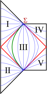
Figure 1: Penrose diagram for the Lorentzian continuation of the CDL instanton. Region I is an open ($k=-1$) FRW universe which is asymptotically flat. Region IV is asymptotically de Sitter. $\Sigma$ is the conformal 2-sphere defined by the intersection of the light-like infinity of region I and the space-like infinity of region IV. The curves indicate orbits of the $SO(3,1)$ symmetry, which acts on $\Sigma$ as the conformal group.

Our focus will be on region I, which can be thought of as the interior of the expanding bubble of true vacuum. The metric in region I takes the form of a standard infinite open FRW universe

$$ds^{2}=a(T)^{2}(-dT^{2}+dR^{2}+\sinh^{2}R\ d\Omega_{2}^{2}).$$ (1.1)

Under the continuation, the $SO(4)$ symmetry becomes the non-compact symmetry $SO(3,1)$ which acts as spatial isometries on the constant time slices. These time slices are uniform negatively curved hyperbolic geometries ${\cal H}_{3}$, isomorphic to 3-dimensional Euclidean Anti-de Sitter space.

The future boundary of the geometry consists of two portions. One is the space-like boundary of region IV, which is asymptotically de Sitter. The other is the light-like “hat.” We will be especially interested in the intersection of these two which we call $\Sigma$. $\Sigma$ is an asymptotic 2-sphere that really represents spatial infinity in the FRW patch.

The central point about $\Sigma$ is that the $SO(3,1)$ symmetry group acts on it as 2-dimensional conformal transformations. Each time slice is geometrically equivalent to a Euclidean AdS space, and has exactly the same symmetries. This suggests that $\Sigma$ may be the location of a holographic dual description.

The two-sphere $\Sigma$ is really spacelike infinity when viewed from the interior of the open FRW geometry of region I. From the Holographic Principle, it follows that there must exist a boundary description of this region, and it should have its degrees of freedom on $\Sigma$. We have seen that $SO(3,1)$ acts as conformal symmetry on $\Sigma$, and that naturally raises the question of whether field correlators extrapolated to $\Sigma$ might be holographically dual to a (Euclidean) conformal field theory (CFT) in a manner analogous to the familiar AdS/CFT duality. We might hope that such a CFT is the holographic description of the open FRW universe in region I.

If so, there would be a surprising twist. Instead of a $2+1$ dimensional hologram, $\Sigma$ would be a $2$ dimensional Euclidean hologram. Not only would the space-like “depth” direction have to emerge from the CFT, but time would also be emergent. Indeed we will find evidence for such a mechanism in the form of a Liouville field in the boundary theory.

As we will see in the rest of the paper, the fact that the Euclidean geometry of the CDL instanton (a deformed sphere) is compact has a profound consequence for holography. We review the geometry in the next section. Although the FRW region of the Lorentzian geometry has infinite volume, the compactness of the Euclidean space seems to forbid a quantization with a fixed boundary condition, in contrast to the case of AdS space where both the Euclidean and Lorentzian geometries are non-compact.

This will become clear when we study the correlation functions for massless fluctuations in section 3. The correlators in the FRW region which are obtained by analytic continuation from Euclidean space do not decay at large spatial separation. This implies that a non-normalizable mode, which is usually considered to be fixed by the boundary conditions and therefore non-dynamical, is now path-integrated.

Our computation of the graviton correlator is the main evidence that the dual theory is a local 2-dimensional CFT. We find a piece of the graviton correlator which is transverse, traceless, and dimension 2 in the boundary theory. This piece has the right properties to be dual to the energy-momentum tensor of the CFT.

The presence of a non-normalizable graviton mode means that the geometry of the boundary fluctuates. In the dual CFT, we expect that the fluctuations of the boundary geometry are described by a Liouville field, as we explain in section 4. Because of the fluctuating boundary, the bulk theory is similar in some ways to quantum gravity in a closed space. The general formalism to treat such a system is the Wheeler-DeWitt theory, which we review in section 5. Since the metric is a dynamical variable, we cannot treat time as a parameter. Instead, time must be defined in terms of clocks which are part of the dynamical system. A convenient choice of clock that is often used is the scale factor, which ordinarily is monotonically increasing for open FRW universes.

What emerges from our considerations is a new kind of hybrid–a holographic WDW theory–in which bulk information is holographically encoded in boundary degrees of freedom, but in which time emerges as a dynamical degree of freedom as in WDW theory. The Liouville field will play the role of time as does the scale factor in the bulk WDW theory. To allow such an interpretation, the Liouville field should have negative metric, which is well known to be the case in the 2-D gravity coupled to a large number of matter fields. The existence of negative metric fields in the CFT is suggested from the bulk correlator calculated in section 3; it implies that the CFT is not unitary. We will discuss properties of the holographic WDW theory in section 6.

In section 7 we point out that a true vacuum bubble inevitably collides with an infinite number of other bubbles [27]. If the de Sitter space can decay to more than one true vacuum, bubble collisions have a dramatic effect on the boundary $\Sigma$, creating regions which are in a different vacuum. We interpret these as instantons in the dual CFT. We see this as a suggestion that the matter sector of the CFT may contain the entire Landscape as its target space.

We describe a number of open questions in section 8. The details of our calculation of the correlation function are in Appendix A for the case of the scalar field and Appendix B for the graviton.

We work in four bulk dimensions throughout. This is not without consequences. Our preliminary calculations suggest that in any number of bulk dimensions the boundary geometry will fluctuate. But only in a 2-dimensional boundary theory can we describe fluctuations of the geometry in terms of a Liouville field; in higher dimensions the situation is unclear.

1.2 Related Work

The duality that we are proposing is different from the “dS/CFT correspondence,” proposed by Strominger [11]. In dS/CFT, the dual CFT is assumed to be at the 3-dimensional spatial surface at the future infinity of de Sitter space. Although de Sitter correlators have conformally invariant form, the late time behavior should be affected by the nucleation of infinitely many bubbles, and the basis for the duality is not entirely clear [12]. If it exists and makes sense, it describes a global view of cosmology that cuts across causally disconnected regions separated by event horizons. The theory in this paper is more local and describes a single pocket universe that emerges from the local decay of a metastable de Sitter vacuum.

Holographic duals containing gravity have been proposed in various contexts similar but different from ours. It has been noted that if the AdS space is cut off at finite volume, the dual theory should contain gravity, essentially because the gravity on the boundary becomes normalizable and fluctuates [14, 15]. Brane-world models where two cut-off AdS (or Schwarzschild AdS) spaces are patched at the cut-off boundary have been studied from the perspective of holographic duality. The holographic dual theory on the brane contains gravity. Fairly concrete analyses have been done in [15, 16].

In [17], an intersting proposal was made for an approximate holographic description for a causal patch of de Sitter space. On the basis of an observation that the limit of de Sitter geometry near an observer’s horizon approaches the limit of AdS geomerty far from the boundary, the authors proposed a CFT dual for de Sitter valid in the low energy limit. It is argued that the CFT contains gravity since the geometry where the CFT is expected to live can fluctuate as in the brane-world cases.

There have also been attempts to describe de Sitter space or cosmology using the AdS/CFT correspondence by embedding the spacetime in asymptotically AdS space. Ref. [18] pursues the possibility of extracting information on the bubble of de Sitter space embedded in an asymptotic AdS space from the boundary CFT. Ref [19] studies a model of big crunch in AdS/CFT correspondence.

Our proposed duality has similarities with the proposal of de Boer and Solodukhin [20] for a holographic theory of flat space. They considered the hyperbolic slicing of flat space (a part of it corresponding to our region I), and proposed that a dual theory should be a CFT living on the boundary of the hyperboloid; this is precisely what we do. However, we benefit from having a compact Euclidean geometry. In contrast to [20] where they consider a continuous infinite family of the CFT operators to reconstruct the flat space correlators, we will naturally find a discrete tower of operators in the CFT. In addition, our main focus is on the piece of the correlation function which is absent in flat space.

2 The CDL Instanton

In this section we review vacuum decay via Coleman-de Luccia tunneling, focusing on the simplest case. We imagine a potential which has a false vacuum with positive vacuum energy and a true vacuum with zero vacuum energy.

The scalar field that interpolates between the two vacua, and its potential, will be called $\Phi$ and $V(\Phi)$. The two minima are at field values $\Phi=\Phi_{F}$ and $\Phi=\Phi_{T}$:

$$V(\Phi_{F}) > 0$$ (2.1)

$$V(\Phi_{T}) = 0.$$ (2.2)

The Euclidean signature CDL instanton geometry has the topology of a 4-sphere. It is described by the metric

$$ds^{2}=dt^{2}+a(t)^{2}d\Omega_{3}^{2}$$ (2.3)

where $d\Omega_{3}^{2}$ is the metric of a unit 3-sphere. The Euclidean equations of motion are

$$\left({\dot{a}\over a}\right)^{2} = \ {1\over 2}\dot{\Phi}^{2}-V(\Phi)+{1\over a^{2}}$$ (2.4)

$$\ddot{\Phi} = -3{\dot{a}\over a}\dot{\Phi}+{\partial V\over{\partial\Phi}}.$$ (2.5)

The Euclidean time runs from $t=0$ to $t=t_{0}$ and the boundary conditions are

$$\dot{a} = 1,\ \ \ \ \ (t=0)$$ (2.6)

$$\dot{a} = -1,\ \ \ (t=t_{0})$$ (2.7)

$$\dot{\Phi} = 0,\ \ \ \ \ (t=0,\ \ t=t_{0}).$$ (2.8)

The most important features of the instanton geometry are its topology, $S^{4}$, and its symmetry, $SO(4)$. Note that in general the $SO(5)$ symmetry of $S^{4}$ is broken. The $SO(4)$ acts on the 3-sphere $\Omega_{3}$.

It will be convenient to change variables from $t$ to a “conformal” variable $X$ defined by

$$dX={dt\over a(t)}~{}.$$ (2.9)

In terms of $X$, the metric becomes

$$ds^{2}=a(X)^{2}(dX^{2}+d\Omega_{3}^{2})~{}.$$ (2.10)

The variable $X$ runs over the entire real axis and the equations of motion become

$$(a^{\prime})^{2} = {1\over 2}a^{2}(\Phi^{\prime})^{2}-a^{4}V(\Phi)+a^{2}$$ (2.11)

$$\Phi^{\prime\prime}+{2a^{\prime}\Phi^{\prime}\over a} = a^{2}{\partial V\over\partial\Phi},$$ (2.12)

where prime indicates derivative with respect to $X$.

As described in the introduction, the continuation to Minkowski signature defines the bounce geometry, which is relevant after the tunneling event. In order to continue the Euclidean CDL geometry to region I of the Minkowski geometry (see figure 1), we write the 3-sphere metric in the form

$$d\Omega_{3}^{2}=d\theta^{2}+\sin^{2}{\theta}d\Omega_{2}^{2}.$$ (2.13)

The continuation is defined by

$$X \to T+{\pi\over 2}i$$ (2.14)

$$\theta \to iR.$$ (2.15)

The metric in region I is an open FRW universe,

$$ds^{2}=a(T)^{2}(-dT^{2}+dR^{2}+\sinh^{2}R\ d\Omega_{2}^{2})=a(T)^{2}(-dT^{2}+d{\cal H}_{3}^{2})$$ (2.16)

The $SO(3,1)$ symmetry is realized on the hyperboloid ${\cal H}_{3}$. ${\cal H}_{3}$ is equivalently a 3-dimensional Euclidean AdS space. Defining $\Sigma$ to be the boundary of ${\cal H}_{3}$, it is clear that the symmetries act on $\Sigma$ as the conformal group, just as in the AdS/CFT correspondence.

3 Correlation Functions

The basis for our conjecture is the properties of correlation functions of ordinary bulk fields in the bounce geometry. The method of calculation is to begin with correlation functions defined on the original Euclidean CDL geometry. Analytically continuing the Euclidean correlation functions to Minkowski signature then allows us to extrapolate them to $\Sigma$. One can then ask if the correlation functions have the properties required of fields in a CFT. The method of calculation is explained in detail in Appendix A for scalars, and in Appendix B for gravitons. In this section we will discuss the general features. Since we compute the correlators by analytic continuation from Euclidean space, what we are doing is computing expectation values in the Hartle-Hawking state [13]. Because we are computing expectation values of Hermitian operators with arguments at space-like separated points, our answers are guaranteed to be real. This fits well with the dual CFT, which we expect to be a Euclidean theory. As we will see, the bulk correlators can be interpreted as correlators of CFT operators with real dimensions.

We examine the correlators in a particular limit. We believe that the CFT should be closely related to the late time asymptotics of the correlators, where particles become non-interacting; we think of the CFT as describing the “out” state. So we want to take the limit $T\to\infty$. Furthermore, as usual it is useful to think of the CFT as living on the boundary $R\to\infty$ of AdS space, in this case $\Sigma$, so we want to expand the correlators for large $R$. To be precise, we look at the correlators in the limit

$$T+R\to\infty$$ (3.1)

and in an expansion which is valid for large $R-T$.

3.1 Massless Scalar

We will begin with the simplest case of a minimally coupled massless bulk scalar field $\chi$, then move to the case of the graviton. We can make use of the symmetries to write the correlator as a function of a few variables. Recall that the metric in region I is

$$ds^{2}=a(T)^{2}(-dT^{2}+d{\cal H}_{3}^{2}).$$ (3.2)

The $SO(3,1)$ symmetry means that the correlator cannot depend arbitrarily on the location of the two points in the hyperboloid ${\cal H}_{3}$; it must be a function of only one parameter, which we take to be the geodesic distance $\ell$ on the unit hyperboloid. The correlator can depend on the two time coordinates in an arbitrary way because we have no time translation invariance.

We are primarily interested in the piece of the correlator which has non-trivial dependence on $\bar{T}=T_{1}+T_{2}$. This piece does not exists in the flat space; it essentially corresponds to the particle production due to the geometry.

Calculation of the Euclidean correlator boils down to a one-dimensional Schrödinger problem, and the $\bar{T}$ dependent piece is written in terms of the reflection coefficient ${\cal R}(k)$. In Appendix A we derive an expression for the Lorentzian correlator in the form of a contour integral,

$$\langle\chi(T_{1},0)\chi(T_{2},R)\rangle^{(\bar{T})}=e^{-\bar{T}}\oint_{C}{dk\over 2\pi}{\cal R}(k)e^{-ik\bar{T}}{\left(e^{-ikR}-e^{ikR-2\pi k}\right)\over 2\sinh R\sinh k\pi},$$ (3.3)

where we have placed one of the points at the origin of the hyperboloid, so that the geodesic distance is $\ell=R$. The last factor comes from the Green’s function on $S^{3}$, which we rotate to ${\cal H}_{3}$.

In the limit of interest, the two terms in the integrand are evaluated on different contours. The first term is closed in the lower half plane, as in Figure 2(b), while the second term is closed in the upper half plane, as in Figure 2(a). The reflection coefficient has a pole at $k=i$, as does $1/\sinh(k\pi)$, so there is a double pole at $k=i$. This double pole is ultimately due to the zero mode in Euclidean space. The factor $1/\sinh(k\pi)$ gives rise to single poles at integer multiple of $k=i$, and the correlator is written as a sum of an infinite number of terms.

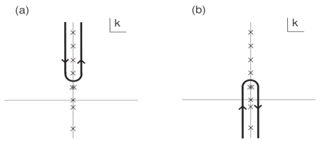
Figure 2: (a) Contour surrounding single poles at $k=2i,3i,\ldots$. (b) Coutour surrounding a double pole at $k=i$, single poles at $k=0,-2i,-3i,\ldots$, and a single pole at $k=-ia$ $(0<a<1)$ which is due to the pole of ${\cal R}(k)$; for the “half-sphere” example in Appendix A.2, $a=1/2$. There is no pole at $k=-i$ since ${\cal R}(k)$ has a zero there.

The correlator consists of two types of terms

$$\langle\chi\chi\rangle=G_{1}(T_{1},T_{2},\ell)+G_{2}(T_{1},T_{2},\ell),$$ (3.4)

as we explain in the following.

3.1.1 Terms with definite dimensions

The first term $G_{1}(T_{1},T_{2},\ell)$ arises from the contour shown in figure 2(a), together with one piece of the double pole contained in the contour shown in figure 2(b). It has the form

$$G_{1}=\sum_{\Delta=2}^{\infty}G_{\Delta}~{}e^{(\Delta-2)(T_{1}+T_{2})}~{}{e^{-(\Delta-1)\ell}\over\sinh\ell}$$ (3.5)

where the $G_{\Delta}$ are constants. The motivation for the unusual label $\Delta$ for the summation variable will become clear in a moment. This formula has an interesting interpretation. Each term in the sum is the product of a time-dependent piece and a piece which depends on the separation of the points on the hyperboloid ${\cal H}_{3}$. The latter,

$${e^{-(\Delta-1)\ell}\over\sinh\ell}~{},$$ (3.6)

is exactly the correlation function for a (fictitious) 3-dimensional AdS bulk field of mass

$$m^{2}=\Delta(\Delta-2)$$ (3.7)

in Euclidean AdS. So the correlator appears to consist of an infinite series of terms, each corresponding to a field with definite mass in Euclidean AdS.

As usual, the mass of a field in AdS translates into the conformal dimension in the dual CFT. To see the relationship, note that the geodesic distance $\ell$ can be expressed in terms of $R_{1},R_{2},\Omega_{1},\Omega_{2}$. In the limit that the $R$’s tend to infinity (the limit in which the points tend to $\Sigma$), $\ell$ has the form

$$\ell\to R_{1}+R_{2}+\log(1-\cos\alpha),$$ (3.8)

where $\alpha$ is the angle between the points on the 2-sphere. The correlator (3.5) can be rewritten in this limit

$$e^{(\Delta-2)(T_{1}+T_{2})}{e^{-(\Delta-1)\ell}\over\sinh\ell}\to e^{(\Delta-2)(T_{1}+T_{2})}e^{-\Delta R_{1}}e^{-\Delta R_{2}}(1-\cos{\alpha})^{-\Delta}.$$ (3.9)

Apart from the time dependent factors, these expressions are familiar from the AdS/CFT duality where they represent correlation functions of boundary conformal fields of dimension $\Delta$. The factors $e^{-\Delta R}$ are wave function renormalization factors and the angular dependence $(1-\cos{\alpha})^{-\Delta}$ is the renormalized two point function of a field of dimension $\Delta$. The obvious interpretation is that the boundary theory has an infinite number of conformal fields of dimension $\Delta=(2,3,4....)$. In particular the lowest dimension field has dimension $\Delta=2$. Note that the dimension of the Lagrangian of a 2-D CFT is 2.

Defining the light-cone variables

$$T^{+} = T+R$$ (3.10)

$$T^{-} = T-R,$$ (3.11)

and combining (3.5) and (3.9) we can write the correlator in the form

$$e^{-(T^{+}_{1}+T^{+}_{2})}\sum_{\Delta}G_{\Delta}e^{(\Delta-1)(T^{-}_{1}+T^{-}_{2})}(1-\cos{\alpha})^{-\Delta}.$$ (3.12)

The characteristic behavior of this term is simple: it has an overall factor $e^{-T^{+}}$ for each external “leg.” If we strip off that factor the remaining expression has a smooth limit as we approach the hat at $T^{+}=\infty$. The remaining factor is a sum of discrete contributions that can be identified with correlators of definite dimension $\Delta$.

Equation (3.12) suggests a strategy for connecting the CFT correlators to the correlators on the hat. These correlators are roughly analogous to S-matrix elements involving massless outgoing particles. Equation (3.12) suggests that each bulk scalar field be identified with an infinite sum of boundary conformal fields,

$$\lim_{T^{+}\to\infty}\ e^{T^{+}}\chi=\sum_{\Delta}e^{(\Delta-1)T^{-}}\chi_{\Delta}.$$ (3.13)

3.1.2 Logarithmic terms

The second term $G_{2}$ arises from the double pole at $k=i$. It is more difficult to interpret. It has the form

$$G_{2}={e^{\ell}\over\sinh\ell}(T_{1}+T_{2}+\ell),$$ (3.14)

which for large $R_{1},R_{2}$ behaves like

$$G_{2}\sim(T_{1}+T_{2}+R_{1}+R_{2}+\log(1-\cos\alpha)).$$ (3.15)

We will interpret this as follows. The minimally coupled massless scalar has a translation symmetry $\chi\to\chi+\chi_{0}$ where $\chi_{0}$ is a constant. Interpreting this as a gauge symmetry, the gauge invariant quantities are derivatives of $\chi$. Thus we are really interested in derivatives of the correlator of the form

$$\partial_{1}\partial_{2}G_{2}.$$ (3.16)

It is evident from (3.15) that only the last term contributes when we differentiate with respect to both arguments of $G$. Thus for gauge invariant purposes we may replace (3.15) by the simpler form

$$G_{2}=\log(1-\cos\alpha).$$ (3.17)

The expression in (3.17) has a familiar significance. $G_{2}$ is exactly the correlation function of a massless dimension-zero scalar field in the boundary theory.

However, from the bulk point of view, something unusual is happening. The behavior (3.15) indicates that the fluctuation of $\chi$ contains non-normalizable modes on the hyperbolic space ${\cal H}_{3}$. In AdS space such modes are associated with boundary conditions and not dynamical degrees of freedom. What we are finding is that the infrared behavior of the correlation function describes not only normalizable quantum fluctuations in the background FRW universe, but also fluctuations of the asymptotic boundary conditions. In other words the infrared behavior of the correlation contains information about a measure on the space of asymptotically different pocket universes.

From the form of (3.14) we see that there is a sub-leading term. Writing

$${e^{\ell}\over\sinh\ell}=2+{e^{-\ell}\over\sinh\ell},$$

we see that the sub-leading term in the limit $R\to\infty$ behaves like

$$\left[T_{1}+T_{2}+R_{1}+R_{2}+\log(1-\cos\alpha)\right]e^{-2\ell}$$ (3.18)

Apart from the factor $[(T_{1}+T_{2}+R_{1}+R_{2}+\log(1-\cos\alpha)]$ this is the correlator for a dimension 2 field. Evidently, this term is corrupting the dimension 2 piece of the correlator with a prefactor that tends to infinity. If we make the usual connection between the radial variable $R$ and scale-size in the boundary theory, then the prefactor would represent a logarithmic running of the correlation function.

3.2 Separating the Double Pole

In fact the logarithmic behavior associated with (3.14) is probably not present in the correlator of a realistic scalar field. It is associated with the infrared divergences of a massless minimally coupled (MMC) bulk field in the compact Euclidean CDL geometry–divergences due to the zero mode of the field. Now MMC scalars may exist in the final vacuum with zero cosmological constant. Indeed the only such vacua in string theory are on the supersymmetric moduli space and the moduli themselves are MMC scalars. But one expects that in a stable de Sitter vacuum the moduli will be fixed. Thus one should allow the scalar field to have a mass in the false vacuum. The effect of adding such a mass is to split the double pole at $k=i$ into a pair of single poles at $k=i$ and at $k=i(1-\epsilon)$. The result is the following (more details in Appendix A.4):

1) For small mass the logarithmic term (3.14) is replaced by a term with positive dimension equal to $\epsilon$. As the mass increases the dimension also increases until it approaches dimension $\epsilon=1$ at some threshold mass. Beyond that mass, the pole moves to the lower half plane and ceases to contribute to the correlator in our limit.

2) The corrupted dimension $2$ term splits into two contributions, each with definite dimension. One term coming from the pole at $k=i$ has dimension $2$. The other term moves to $\Delta=2+\epsilon$.

Our conclusion from this latter result is that there are two distinct terms with $\Delta=2$ and $\Delta=2+\epsilon$ which “accidentally” become degenerate as the mass term is switched off.

3.3 Gravitational Correlators

The description of bulk gravitational fluctuations $h_{\mu}^{~{}\nu}$ in the transverse traceless gauge is very similar to the case of the MMC scalar. Much of the analysis of that case carries over. In Appendix B we calculate the two point function $\langle h_{\mu}^{~{}\nu}h_{\mu^{\prime}}^{\ \nu^{\prime}}\rangle$. Since the symmetry of the problem acts on ${\cal H}_{3}$, we decompose the graviton in representations on ${\cal H}_{3}$; our interest is in modes which are transverse and traceless on ${\cal H}_{3}$. Here we quote the results from Appendix B.

As in the scalar case, the correlator contains two terms, one essentially identical to (3.5) except that the constants $G_{\Delta}$ are replaced by bi-tensors describing the index structure. As in the scalar case the leading dimension is 2. We find a dimension 2 piece which is transverse-traceless not only in the three-dimensional bulk space but also in the two dimensional boundary sense. In other words if we define the indices on the asymptotic 2-sphere $\Sigma$ to be $i,j$, then this dimension 2 piece satisfies

$$\nabla_{i}\langle h^{i}_{~{}j}h^{k}_{~{}l}\rangle_{(2)} = 0$$ (3.19)

$$\langle h^{i}_{~{}i}h^{k}_{~{}l}\rangle_{(2)} = 0.$$ (3.20)

Apart from a numerical factor of proportionality, this piece is a candidate for the energy-momentum tensor of the boundary theory. The equations (3.20) become conservation and tracelessness of the stress tensor.

As in the scalar case we find a term in the correlation function which is similar to (3.15). The correct expression is given in equations (B.20) and (B.21). Once again, to get a gauge invariant quantity, we need to take derivatives of the correlator. Let us consider the fluctuation of the curvature invariant of the asymptotic 2-sphere

$$C(\Omega_{2})=\partial_{i}\partial^{j}h_{j}^{i}.$$ (3.21)

Explicit calculation shows that the correlation function of the two dimensional curvature satisfies

$$\langle CC\rangle=(1-\cos{\alpha})^{-2}$$ (3.22)

so that the curvature is an operator of dimension 2.

The curvature fluctuations of the boundary sphere are of the same order of magnitude as the background curvature. The meaning of this is that the shape of the asymptotic 2-sphere–its oblateness for example–has finite fluctuations even as $R$ and $T$ go to infinity. Note that by contrast, in AdS space, the fluctuations of the shape of the boundary go to zero for all finite energy configurations. Another way to say the same thing is that in AdS the dynamical quantum fluctuations of the space are composed of normalizable modes while in the present case non-normalizable modes also fluctuate.

The fluctuations of the intrinsic geometry of the boundary $\Sigma$ require us to replace $d\Omega_{2}^{2}$ in (1.1), with

$$e^{L(\theta,\alpha)}d\Omega_{2}^{2}$$ (3.23)

where $L$ is a Liouville field [26] on $\Sigma$. The existence of a Liouville field in the boundary theory clears up a mystery. Ordinarily, holographic theories are $D-1$ dimensional with one of the dimensions being time. But in the present case we are proposing a $D-2$ dimensional Euclidean holographic dual. We have lost a dimension but gained a Liouville field.

Now let’s return to the dimension $2$ piece of the correlator. As in the scalar case there are logarithmic terms that corrupt the pure $\Delta=2$ term, once again from a double pole at $k=i$. If we split the double pole into single poles, then as in the scalar case, we find two operators. The one at $\Delta=2$ is transverse-traceless in the boundary directions but the shifted one at $\Delta=2+\epsilon$ is not. It is the former that we identify with the stress tensor of the boundary theory.

The logarithmic factor for the dimension 2 piece is a result of the degeneracy of the $\Delta=2$ piece and $\Delta=2+\epsilon$ piece which have opposite signs. The term with negative sign in the correlator implies the presence of a field with negative metric in the CFT. This is what we want. We expect the Liouville field to be a negative metric field since we want to interpret it as time; the Liouville field can have negative kinetic term when there are large number of matter fields. The existence of a field with negative kinetic term suggests that the CFT is non-unitary.

4 The Holographic Correspondence

In the usual AdS/CFT duality the extra bulk direction of space corresponds to scale size in the CFT [21, 22]. In Poincare coordinates the spatial metric is

$$ds^{2}=a^{2}{dz^{2}+dx^{i}dx^{i}\over z^{2}}$$ (4.1)

where $a$ is the overall radius of the AdS space, $x^{i}$ are the coordinates in the plane of the boundary, and $z$ is the emergent radial coordinate.

It is well known that the image of a point located at $z$ is a patch on the boundary of coordinate size

$$\Delta x=z.$$ (4.2)

Thus we see that scale size in the CFT is dual to the emergent coordinate $z$. Equivalently we can write

$$\Delta x=e^{-R}.$$ (4.3)

Thus the coordinate $R$ is logarithmically related to scale size in the boundary theory

$$R=-\log{\Delta x}$$ (4.4)

Now let us regulate the boundary sphere by locating it at finite $R$. More exactly, let the boundary be at a variable radial distance given by

$$R=R(\Omega_{2}).$$ (4.5)

This is not enough to define the regulated sphere because all the constant $T$ surfaces intersect on $\Sigma$.

Let us compare the situation with AdS/CFT. In that case the emergent direction of space would correspond to $R$, the spatial direction perpendicular to $\Sigma$. In fact $e^{-R}$ is identified with scale size in the CFT. The geometric arguments for that identification should go over into the present case. But now consider the fact that $\Sigma$ is really a place where all time slices intersect. Specifying a large sphere involves not only choosing a large value of $R$ but also a value of FRW time. In fact we can introduce a local time at each point of the sphere, $T(\Omega_{2})$, or $T(\theta,\alpha)$. From (1.1) and the fact that

$$a(T)\sim e^{T},$$ (4.6)

we see that the metric of the asymptotic 2-sphere is proportional to

$$e^{2T(\theta,\alpha)}d\Omega_{2}^{2}.$$ (4.7)

Comparing (3.23) and (4.7) we see that there is a natural identification of the Liouville field with local time,

$$L(\theta,\alpha)=2T(\theta,\alpha).$$ (4.8)

5 Wheeler-DeWitt Theory

As in the case of anti-de Sitter space, the spatial slices of open FRW are negatively curved hyperbolic planes with a boundary at spatial infinity. In the present case that boundary is the infinite 2-sphere $\Sigma$. It is entirely natural to expect that a holographic description of open FRW lives on this boundary. However there is one big difference between open FRW and AdS. It is not that the background is time dependent in the FRW case. Time dependence can easily be introduced into the AdS/CFT correspondence, for example by varying the value of the gauge coupling constant in a time dependent way. More important is that in the AdS case the boundary conditions at spatial infinity are frozen. To vary the boundary conditions requires exciting the non-normalizable modes which always costs infinite energy. By contrast, the boundary conditions in open FRW are not frozen.

The fact that spatial infinity is not frozen has implications for the way we think about time. Unlike AdS we cannot define a global time variable by introducing synchronized clocks at infinity. It follows that a precise notion of global energy such as ADM energy does not exist. Not even a time dependent global Hamiltonian makes sense. What option do we have to define a quantum mechanics of open FRW?

The answer in our opinion is to construct a new kind of hybrid of the Wheeler-DeWitt theory [23] and the Holographic Principle. Let us begin with a quick review of the Wheeler-DeWitt theory. One begins with the Einstein equations. Define

$$E^{\mu}_{~{}\nu}=R^{\mu}_{~{}\nu}-{1\over 2}\delta^{\mu}_{~{}\nu}R-\kappa T^{\mu}_{~{}\nu}.$$ (5.1)

Four of the equations are considered to be constraints that act on the Wheeler-DeWitt wave function

$$E_{~{}a}^{0}\Psi(g_{ab},f) = 0$$ (5.2)

$$E_{~{}0}^{0}\Psi(g_{ab},f) = 0.$$ (5.3)

The wave function $\Psi$ is a functional of the space-space components of the metric $g_{ab}$ and the matter fields which we summarize by $f$. The mixed space-time components are somewhat trivial and merely state that the wave function is invariant under spatial reparameterizations. The time-time equation is the interesting one that contains all the dynamics. It can be written as

$$H\Psi(g_{ab},f)=0$$ (5.4)

where $H$ is the Hamiltonian density derived from the gravitational and matter action.

Typically there are many solutions to the Wheeler-DeWitt equations corresponding to different boundary conditions but the interesting point is that the wave functions are independent of time. They depend only on spatial geometry and matter fields. Any sense of time and temporal evolution must be emergent.

There are many ways to extract time from the Wheeler-DeWitt wave function by identifying some dynamical variable as a clock. The most common is to use the FRW scale factor which in conventional cosmology is a monotonic function of time. The logic is nicely illustrated in the so called mini-superspace approximation in which all the fields are taken to be spatially homogeneous and the geometry is assumed isotropic. In that case the spatial geometry is characterized by a scale factor $a$.

To derive the Wheeler-DeWitt equation we begin with the Lagrangian

$${\cal{L}}=v\left\{[-a\dot{a}^{2}+ka]+[a^{3}{\dot{f}^{2}\over 2}-a^{3}V(f)]\right\}\ .$$ (5.5)

The constant $k$ is equal to $1$, $0$, or $-1$ for closed, flat, or open spatial geometries, and $v$ is the coordinate volume of space; we are setting all inessential constants equal to $1$, so $v$ is dimensionless. The two terms in square brackets represent the gravitational and matter field action. From this we deduce the Hamiltonian

$$H=-{p_{a}^{2}\over 4av}+{p_{f}^{2}\over 2a^{3}v}+va^{3}V(f)-vka$$ (5.6)

where $p_{a}$ and $p_{f}$ are the momenta conjugate to $a$ and $f$. If we make the identifications

$$p_{a} = -i\partial_{a}$$ (5.7)

$$p_{f} = -i\partial_{f},$$ (5.8)

then the Wheeler-DeWitt equation becomes

$$\left({\partial_{a}^{2}\over 4av}-{\partial_{f}^{2}\over 2a^{3}v}+va^{3}V(f)-vka\right)\Psi(a,f)=0.$$ (5.9)

When supplemented by various boundary conditions the Wheeler-DeWitt equation determines the time independent wave function $\Psi(a,f)$. But the full interpretation of the equation requires one additional ingredient that follows from the Lagrangian–namely

$$\dot{a}={p_{a}\over 2av}.$$ (5.10)

Equation (5.10) provides the connection between time and scale factor that allows us to think of the scale factor as a clock. The physics is illuminated by first solving (5.9) setting the matter energy to zero. We will first illustrate the method in the flat case $k=0$ (a torus geometry for example) and with the matter energy being replaced by a cosmological constant

$$\left({\partial_{a}^{2}\over 4av}+va^{3}\lambda\right)\Psi(a)=0.$$ (5.11)

There are two independent solutions corresponding to expanding ($\dot{a}>0$) and contracting ($\dot{a}<0$) universes. The expanding solution, for large $a$ is given by

$$\Psi=e^{ica^{3}v}.$$ (5.12)

where the constant $c$ is given by $c=2\lambda^{{1\over 2}}/3$.

Now if we reinstate the matter field and write

$$\Psi=e^{ica^{3}v}\psi(a,f)$$ (5.13)

we find that for large $a$ (5.9) reduces to the conventional Schrödinger equation

$$-i\partial_{t}\psi(a,f)=H_{matter}\psi.$$ (5.14)

with the role of time being played by $\log{a}$; in the semi-classical limit, the relation (5.10) implies $\dot{a}=3ca/2$, which is given by evaluating (5.10) on the state (5.12).

Beyond the mini-superspace context the single clock represented by the scale factor is replaced by local clocks. For example, the determinant of the space-space metric defines a local scale factor by

$$|g|\to a(x)^{6}.$$ (5.15)

The local scale factor provides a local clock at each point of space. We may also define a global clock by averaging the local clock over space.

Note that in (5.12), the exponent in $\Psi$ is proportional to the volume of space $a^{3}v$. We can obtain this wave function alternatively by dividing space into cells with volume $v_{\rm\scriptsize cell}$, and using the mini-superspace approximation for each cell. The leading term in the wave function at large $a$ will be the direct product of the wave functions for single cells

$$\Psi=\exp({\sum_{\rm\scriptsize cells}ica^{3}v_{\rm\scriptsize cell}})\ .$$ (5.16)

The exponent is now proportional to the sum of the volumes of each cell, so again it is proportional to the total volume of space.

In the open negatively curved FRW universe without cosmological constant, there is a qualitative difference. This time the WDW equation for large $a$ is

$$\left({\partial_{a}^{2}\over 4av}+va\right)\Psi(a)=0,$$ (5.17)

and the wave function for an expanding universe has the form

$$\Psi\sim e^{2ia^{2}v}.$$ (5.18)

Again, let us divide the space into cells to illustrate the point. For simplicity, let us assume that the cells have the coordinate size equal to the curvature radius of the hyperboloid. The leading behavior of the wave function would be the direct product

$$\Psi\sim\exp({\sum_{{\rm\scriptsize cells}}2ia^{2}})\ .$$ (5.19)

The sum appearing in the exponent of (5.19) is odd. Each term is the area of the particular cell (in Planck unit). Adding up areas over the volume of space is an unusual operation. Adding up volumes gives the total volume but adding up areas has no sensible meaning–except in hyperbolic space. To see the point, first regulate the space by giving it a boundary at some large radius $R$. The point about hyperbolic space is that almost all of the cells are near the boundary. The sum is dominated by cells within the radius of curvature of the boundary. Adding up their area simply gives the area of the regulated boundary. Thus the WDW wave function has a distinctly holographic flavor. For late time (large $a$) it has the form

$$\Psi\sim e^{i\alpha({\rm\scriptsize Area})}\ ,$$ (5.20)

where $\alpha$ is a number of order one and the area is measured in Planck units.

For further details on the Wheeler-DeWitt formulation and the emergence of time we refer the reader to [24] and especially [25].

6 Holographic Wheeler-DeWitt Theory

According to the Holographic Principle the degrees of freedom describing a region of space can be identified with the region’s boundary. In the familiar cases like AdS, the boundary is frozen in the sense that it takes an infinite energy to excite the non-normalizable modes that have support at the boundary. The conceptual importance of this fact is that one can always imagine adding distant physical clocks to the system without perturbing the interesting physics deep in the interior. These asymptotic clocks provide the definition of time that forms the basis for the ADM formalism in which the Hamiltonian is a surface integral. In AdS, it is the ADM Hamiltonian which becomes identified with the Hamiltonian of the dual holographic boundary theory.

The present case of open FRW is different. As we have seen the boundary geometry is not frozen. The only way to introduce asymptotic clocks is to build them out of the asymptotic degrees of freedom already present in the system. An obvious candidate for a local boundary clock is the local scale factor, i.e., the Liouville field. We therefore propose the following scheme.

Assume that the boundary $\Sigma$ is equipped with a set of fundamental holographic degrees of freedom whose precise nature is unknown. We would expect that these degrees of freedom would transform nontrivially under some type of gauge transformations and that only gauge invariant combinations would correspond to limits of bulk fields. Among the degrees of freedom, or perhaps composed out of them, is a Liouville field $L(\Omega_{2})$. For simplicity we label the fundamental holographic fields as ($L,f$).

We also assume that there is a local generator of time translations on $\Sigma$ that has the form of a Hamiltonian density $\hat{H}(\Omega_{2})$ and a Wheeler-DeWitt wave function $\hat{\Psi}(L,f)$ satisfying

$$\hat{H}\hat{\Psi}=0.$$ (6.1)

The quantity $\hat{\Psi}^{{\dagger}}\hat{\Psi}$ defines the measure for computing expectation values of functions of $L$ and $f$. With no loss of generality we can write

$$\hat{\Psi}^{{\dagger}}\hat{\Psi}=\exp\left\{-S(L,f)\right\}.$$ (6.2)

In other words the functional $S(L,f)$ defines an action for a 2-dimensional Euclidean CFT on $\Sigma$. However what we don’t know is whether $S$ has the form of a local action, i.e., an integral of a local density.

6.1 Locality?

Is there reason to hope that the holographic WDW wave function might be local in the above sense? It is difficult to prove or disprove, but the following argument might be suggestive.

Let us consider a regulated version of the theory with a boundary placed at a finite distance $R$. Let $\alpha$ be an angle on the sphere and let us measure time by the conformal time $T$.

From the form of the open FRW metric one sees that the coordinate speed of light on the boundary sphere tends to zero like $e^{-R}$. We see this as a suggestion that the spatial derivative terms in the boundary Hamiltonian $\hat{H}$ must also tend to zero. One could locally undo this slowing down by re-scaling the space coordinate on the sphere by a compensating factor.

Now (for finite $R$) we write the WDW wave function in the form (6.2). Cluster decomposition requires $S$ to have the form of an integral over $\Sigma$ of connected clusters (monomials) where the coefficient functions in the clusters tend to zero at large separation. But as $R$ tends to infinity the coordinate size of the clusters shrinks due to the re-scaling of the velocity of light. This suggests that the wave function may become local.

On the other hand, the final correlation functions that we would obtain from the wave function are not local. They have short distance singularities but they are not delta functions or derivatives of delta functions. There is no contradiction since a local action can lead to non-local correlations. However, the naive argument about the locality of $\hat{\Psi}$ can be criticized on the grounds that if applied directly to the correlation functions, it would say that they are local.

One interesting point is that the leading term in the bulk wave function is local. As we saw in the last section, the wave function has the leading behavior $\exp\{ic({\rm Area})\}$, and the area is the ultralocal integral over $\Sigma$

$${\rm Area}\ \ =\int_{\Sigma}e^{L}.$$ (6.3)

A strict test of locality would be the existence of a local boundary energy-momentum tensor. We have found a candidate whose 2-point function satisfies the crucial conditions of being traceless and transverse, and has the correct operator dimension. However this is far from sufficient. Calculating three-point functions could confirm that operator product expansions involving the boundary stress tensor satisfy the usual conditions.

In what follows we will assume the locality of $S$ without proof.

6.2 Properties of the CFT

The first question about a CFT is “What is its central charge?” This can be read off from the two point function of the energy-momentum tensor but to do so, we need the numerical factor connecting the energy-momentum tensor with the metric fluctuations.

Let us assume that the bulk metric fluctuation is canonically normalized. In that case it has the same units as a canonically normalized scalar. In four space-time dimensions the field has units of inverse length. Consider the value of the two point function on the Euclidean CDL instanton geometry. If we assume the critical bubble is of the same scale as the Hubble radius in the de Sitter space, then the only scale in the problem is the Hubble radius of the false vacuum. We suspect that even if the critical bubble is parametrically small compared to the Hubble radius, our results continue to hold. Let us call the Hubble radius $D$. Evidently the two point function must scale like

$$\langle hh\rangle\sim D^{-2}.$$ (6.4)

Now let us assume that the 2-dimensional $T_{~{}\mu}^{\nu}$ is proportional to the boundary value of $h$. Schematically

$$T=qh$$ (6.5)

with $q$ a numerical constant. It follows that the short distance singularity in $\langle TT\rangle$ will have strength

$$\langle TT\rangle\sim q^{2}/D^{2}.$$ (6.6)

Next consider the 3-point function $\langle hhh\rangle$. One thing we know about it is that it contains a gravitational coupling constant $\kappa$ with units of length. We also know that it has dimensions of inverse length cubed. Thus it must be of order

$$\langle hhh\rangle\sim\kappa/D^{4}$$ (6.7)

and

$$\langle TTT\rangle\sim q^{3}\kappa/D^{4}.$$ (6.8)

Finally, we use the fact that the ratio of the two and three point function is controlled by the classical algebra of diffeomorphisms. Schematically $[T,T]=T$. This implies that the ratio of the two and three point function is parametrically independent of $D$ and $\kappa$. Thus

$$q\sim D^{2}/\kappa$$ (6.9)

and the two point function is of order

$$\langle TT\rangle\sim D^{2}/\kappa^{2}=D^{2}/G$$ (6.10)

The implication is that the central charge is of order the entropy of the parent de Sitter space that gave birth to the open FRW by CDL tunneling.

In a Liouville theory the central charge is not a measure of the number of degrees of freedom of the system. One can see that in the semiclassical limit in which the total central charge can be written as a sum of a Liouville term $c_{L}$, and a matter term $c_{M}$. Typically (and we will assume it here) the matter central charge is positive and represents the number of matter degrees of freedom. But the Liouville central charge can be negative, especially when the Liouville field represents a time-like coordinate.

Assuming that the Liouville theory can be decomposed into a 2-D gravitational sector and a 2-D matter sector, one can ask if the matter sector is conformal. The coupling of Liouville to a conformal field theory has especially simple properties that make it easy to study. However any such theory has an extra Weyl invariance that can be interpreted as unbroken translation invariance of the Liouville field. That would imply time-translation ($T$ translation) invariance which is not something we expect in a cosmological theory.

One direct way to see that the matter sector is not conformal is from the curvature-curvature correlator (3.22). When Liouville is coupled to conformal matter, the two sectors decouple and the Liouville field satisfies a field equation that implies no fluctuation in the curvature. When coupled to non-conformal matter, the curvature (more precisely, the Euler density, $\sqrt{g}R$) becomes a fluctuating field with dimension $2$. Evidently (3.22) implies that the matter sector in not conformal.

It is clear that there is a kind of Infrared/Ultraviolet connection in the system. The Liouville degree of freedom can be identified with the logarithm of the ultraviolet regulator scale. Since the Liouville field is identified with time, it is evident that the late time behavior of the FRW universe is controlled by the UV behavior of the CFT.

What is the UV behavior of the matter theory? The Holographic Principle suggests an answer. The maximum entropy in a bulk region of fixed radius–say $R$– is proportional to the proper area of the boundary

$$S_{max}\sim e^{2R}e^{2T}.$$ (6.11)

On the boundary theory side the number of degrees of freedom can be estimated in a manner analogous to the method used in [21]  but with some modifications required by the Liouville field. As in [21], one first regulates the theory by introducing a coordinate length scale $\delta$ on the boundary sphere. The cutoff $\delta$ is not a proper-distance cutoff. It represents a uniform grid size on the background unit 2-sphere. If there were no Liouville field, the number of effective degrees of freedom in the cutoff area is of order $c_{m}$. In this counting, a single 2-dimensional Dirac fermion is a single degree of freedom.

However, the existence of a Liouville field modifies this formula so that the number of degrees of freedom is

$$N_{dof}\sim c_{m}\delta^{-2}e^{L}.$$ (6.12)

If the matter theory is not conformal, then $c_{m}$ should be thought of as a scale dependent quantity.

In [21] it was explained that an ultraviolet cutoff in the CFT is equivalent to an infrared cutoff on the radial coordinate $R$. The cutoffs are related by

$$\delta=e^{-R}.$$ (6.13)

Evidently, matching the number of degrees of freedom of the Liouville theory with the number expected from the Holographic principle, requires $c_{m}$ to tend to a constant in the ultraviolet. This means that the matter theory is governed by a fixed point in the UV.

At the moment that is all we know about the matter theory but we hope to come back to it.

7 Boundary Instantons and Bubble Collisions

We have assumed that the world can be described by a single CDL bubble. However, Guth and Weinberg long ago showed that the isolated pocket universes that are produced by eternal inflation are in fact infinite clusters of colliding bubbles [27]. In this section we will discuss the implications of such collisions for the holographic boundary description.

To understand why bubbles must occur in infinite clusters consider a time-like trajectory in pure de Sitter space that ends at the future boundary. Assume that there is a finite probability per unit proper time for a bubble to nucleate and engulf the trajectory. Then, since the trajectory is infinite, it is certain that a bubble will nucleate before the trajectory reaches the future boundary. This is shown in Figure 3 (top figure).

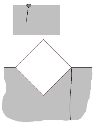
Figure 3: Top: Time-like trajectory that ends up in a bubble. Bottom: Time-like trajectory that meets a flat-space bubble at $\Sigma$. Since infinitely many bubbles, which are not drawn here, form in de Sitter space, this trajectory will inevitably be caught in another bubble like the one in the top figure.

Now consider the time-like trajectory that intersects the future boundary at $\Sigma$ (bottom of Figure 3). The proper time of such a trajectory is infinite so that it is certain that a bubble nucleates along it. Such a bubble will definitely collide with the original bubble. When bubbles collide they in effect form a single bubble but the intersection of the bubble boundary with the future boundary of de Sitter space (we still call that intersection $\Sigma$) will no longer be a geometric sphere. This is another indication that the geometry of $\Sigma$ fluctuates. These fluctuations are clearly non-perturbative since bubble nucleation is a tunneling process.

In order to understand the importance of such processes let us consider a Landscape that includes a key feature, namely a moduli space of vacua with vanishing vacuum energy. In string theory this would be the supersymmetric moduli space (SMS). In general it is possible to decay to different points on the moduli space. In fact we doubt that there are any obstructions to decaying to arbitrary points on the SMS. This means that a given de Sitter vacuum can decay to a variety of bubble-types.

Consider a decay to a point R on the moduli space. Let’s call it the Red point. At a later time (global de Sitter time) a bubble nucleates with the interior at the Blue point B. Assume the two points are connected by massless moduli. The boundary sphere (topologically spherical) $\Sigma$ consists of two regions, one red and one blue. The blue region will be very much smaller than the red if the blue decay is later than the red. On the other hand, in the bulk, the red and blue will bleed into one another and as time evolves the bulk space should evolve to some average color. But the boundary $\Sigma$ remains divided into red and blue.

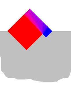
Figure 4: Collision of two flat-space bubbles of different types.

The blue patch in the red background has a natural interpretation in the boundary field theory. It is a localized non-vacuum region with an exponentially suppressed amplitude. In other words it is an instanton.

The statement that the blue vacuum nucleates later than the red is not invariant. There are symmetries of the background de Sitter space that interchange the order of events. This manifests itself in the boundary theory. A conformal transformation of the sphere $\Sigma$ can push the blue region out into the red region and shrink the red to a small patch. Turning an instanton “inside out” is always possible in a conformal field theory.

Another interesting point: a red bubble can nucleate and collide with the blue bubble. This will appear as a red instanton inside the blue instanton.

Figure 5: A red instanton inside a blue instanton.

The integration over instanton sizes is equivalent to the integration over the time at which the associated bubble nucleates. Since one expects the rate of nucleation to be constant, the integration must diverge. The divergence is for small instanton sizes from the CFT point of view. The implication is clear: the average number of instantons must be infinite and be dominated by instantons of arbitrarily small size.

So far we have considered instantons associated with decays onto the moduli space. Let us consider another situation in which the original bubble collides with a bubble of non-zero vacuum energy $\lambda_{2}$ as in Figure 6. The two bubbles, one with vanishing cosmological constant, and one with positive cosmological constant will be separated by a domain wall, and the surface $\Sigma$ will have two portions adjacent to $\lambda_{1}$ and $\lambda_{2}$.

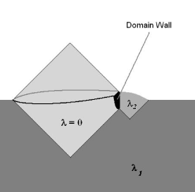
Figure 6: Collision of two bubbles with different cosmological constants.

It appears that instanton gas reflects the diversity of the Landscape. This suggests that the matter sector of the Liouville theory is rich enough to contain, as part of its target space, the entire Landscape including the supersymmetric moduli space as well as all the vacua of non-zero cosmological constant.

We began by considering a transition from a particular de Sitter vacuum to a point on the space of vacua with vanishing cosmological constant. The tentative result is a Liouville theory with central charge determined by the entropy of the false de Sitter vacuum. But then it seems that non-perturbative effects will drive us to a democratic view of the space of vacua; the Liouville theory is associated with the entire Landscape and not just two points. The simplified model of just two points may only be an approximation of a very small part of the theory.

If there is a master Liouville theory of the whole Landscape, then what is its total central charge? We suspect the answer may be zero. Perhaps it is determined by the configuration of maximum vacuum energy, i.e., the Planck energy. A de Sitter space with a Planckian cosmological constant would have vanishing entropy. But obviously this is taking us into very deep waters so we will quit here before we drown.

8 Open Questions

There are a number of questions about our proposal that we left unanswered.

First and foremost is whether the WDW wave function really defines a local conformal field theory. Equation (6.2) defines an action but we don’t know if it is local. An obvious test is to show that the candidate energy-momentum tensor satisfies the usual properties. Thus far we have calculated the two-point function and found it to be traceless, transverse, and of dimension $2$. That is as far as we can go without calculating three-point functions. With three point functions one can test various operator product expansions and also the Schwinger or Virasoro algebra required of a local field theory.

Another question that needs study is what is the effect of vacua with negative cosmological constant. Nucleation of such bubbles leads to singular crunches. What happens when a singular bubble collides with a bubble of zero cosmological constant? Does such a collision give rise to additional instantons?

In our more ambitious interpretation, the CFT would be dual to the entire string theory Landscape. The Landscape includes vacua which are not four-dimensional. What will happen when the four-dimensional universe meets a region with different dimensionality? Does the CFT contain instantons whose interior is effectively higher dimensional?

Finally, what are the degrees of freedom of the boundary theory? Do they derive from some kind of gauge theory? And how does it all fit together with string theory?

Acknowledgements

We would like to thank Raphael Bousso, Eric Gimon, Alan Guth, Simeon Hellerman, Juan Maldacena, Alex Maloney, John McGreevy, and especially Steve Shenker for discussions.

Appendix

Appendix A Scalar correlator in the CDL geometry

In this appendix, we calculate the two-point functions of a scalar field in a 4-dimensional open FRW universe generated by the Coleman-De Luccia (CDL) instanton. The cosmological constant in the true vacuum is assumed to be zero.

We study the correlator of a massless minimally coupled scalar in detail. The main reason for studying this is its similarity with the graviton correlator. Our method for calculating the correlator is to first obtain the correlator on the Euclidean CDL instanton background and then analytically continue the expression to the FRW region (region I of figure 1) of the Lorentzian geometry. This corresponds to taking the Hartle-Hawking vacuum in the bounce solution. Analysis of the scalar correlator in CDL geometry using this method has been done by Gratton and Turok  [28]. (See also refs. [29] for studies of the perturbations the CDL background.)

We will often use the thin-wall approximation. In the thin-wall limit, the Euclidean geometry is a flat disc patched to a portion of a sphere. In this limit, the FRW region of the Lorentzian geometry is exactly a piece of Minkowski space, but the non-trivial geometry in the other regions affects the correlation function. The thin-wall approximation is helpful since we can find the massless scalar correlator exactly. We will derive asymptotic behaviors of the correlators using the thin-wall approximation, but we will argue that the conclusion is true for general CDL geometries.

In section A.1, we explain our prescription for calculating massless scalar correlators. Then in A.2, we present an explicit calculation in a particular thin-wall geometry. We obtain an exact expression for the correlator in A.2.1, and its large distance behavior is studied in A.2.2. In A.2.3, we give an alternative way to derive the asymptotic behavior. In A.3, we discuss asymptotic behavior of the massless scalar correlator in the general CDL geometry. In A.4, we study the case of a scalar field which has finite mass in the false vacuum, as a simple model for realistic moduli fields.

A.1 Euclidean prescription for correlation function

We calculate the two-point function of a massless minimally coupled scalar field $\chi$ in the Euclidean CDL geometry

$$ds^{2}=a(X)^{2}(dX^{2}+d\theta^{2}+\sin^{2}\theta d\Omega_{2}^{2}).$$ (A.1)

The conformal coordinate $X$ varies over $-\infty<X<\infty$. The boundary conditions (2.8) tell us that the scale factor $a(X)$ approaches $c_{-}e^{X}$ as $X\to-\infty$, and $c_{+}e^{-X}$ as $X\to\infty$, with some constants $c_{\pm}$.

It is convenient to consider the rescaled correlator

$$\hat{G}(X_{1},X_{2};\theta)=a(X_{1})a(X_{2})\langle\chi(X_{1},0)\chi(X_{2},\theta)\rangle,$$ (A.2)

which is the correlator of a field $a\chi$ which has the canonical kinetic term. Using the rotational symmetry we have brought one of the two points to $\theta=0$, in which case the correlator depends only on $\theta$ but on no other angular coordinates. The correlator $\hat{G}(X_{1},X_{2};\theta)$ satisfies

$$\left[-\partial_{X_{1}}^{2}+U(X_{1})-\nabla^{2}\right]\hat{G}(X_{1},X_{2};\theta)=\delta(X_{1}-X_{2}){\delta(\theta)\over\sin^{2}\theta},$$ (A.3)

where $\nabla^{2}$ is the Laplacian on $S^{3}$ and $U(X)\equiv a^{\prime\prime}(X)/a(X)$. We have $U(X)\leq 1$ everywhere: It follows from (2.12) that

$${a^{\prime\prime}\over a}-1=-\left({1\over 2}(\Phi^{\prime})^{2}+2a^{2}V(\Phi)\right),$$ (A.4)

and the right hand side is negative since $V(\Phi)\geq 0$ for our case. The asymptotic value of the potential is $U(X)\to 1$ as $X\to\pm\infty$.

Let us obtain $\hat{G}(X_{1},X_{2};\theta)$ in an expansion in the eigenmodes of $[-\partial_{X}^{2}+U(X)]$. Normalizable modes consist of the continuum modes and the bound states. The continuum modes $u_{k}(X)$ satisfy

$$[-\partial_{X}^{2}+U(X)]u_{k}(X)=(k^{2}+1)u_{k}(X)$$ (A.5)

with real $k$. These approach the plane wave asymptotically. The set of orthonormal modes is given by the waves coming from the left and those coming from the right. The modes $u_{k}(X)$ with $k>0$ are defined to be the waves coming in from the left,

$$u_{k}(X)\to e^{ikX}+{\cal R}(k)e^{-ikX}\quad(X\to-\infty),\qquad u_{k}(X)\to{\cal T}(k)e^{ikX}\quad(X\to\infty).$$ (A.6)

where ${\cal R}(k)$ and ${\cal T}(k)$ are the reflection and transmission coefficients; they satisfy ${\cal R}(-k)={\cal R}^{*}(k)$, ${\cal R}(-k)={\cal T}^{*}(k)$, and ${\cal R}(k){\cal R}^{*}(k)+{\cal T}(k){\cal T}^{*}(k)=1$. The modes $u_{-k}$ $(k>0)$ are the ones coming in from the right,

$$u_{-k}(X)\to{\cal T}_{r}(k)e^{-ikX}\quad(X\to-\infty),\quad u_{-k}(X)\to e^{-ikX}+{\cal R}_{r}(k)e^{ikX}\quad(X\to\infty),$$ (A.7)

where ${\cal R}_{r}(k)$ and ${\cal T}_{r}(k)$ are the reflection and transmission coefficients for the incidence from the right. In fact, they are related to ${\cal R}(k)$ and ${\cal T}(k)$ by ${\cal T}(k)={\cal T}_{r}(k)$, ${\cal R}(k)/{\cal R}_{r}(k)^{*}=-{\cal T}(k)/{\cal T}(k)^{*}$. (See e.g. [30] for generalities about one-dimensional scattering.)

There is always a zero-energy bound state $u_{B}(X)\propto a(X)$ which satisfies

$$[-\partial_{X}^{2}+U(X)]u_{B}(X)=0.$$ (A.8)

In terms of the physical field $\chi$, this mode is simply

$$\chi=constant.$$ (A.9)

There is no other bound state, as we will show in section A.3 by using a technique of supersymmetric quantum mechanics. In the case of higher dimensional CDL geometry, the corresponding equation generically has additional bound states.

Using the completeness relation, we rewrite the delta function

$$\delta(X_{1}-X_{2})=\int_{-\infty}^{\infty}{dk\over 2\pi}u_{k}(X_{1})u_{k}^{*}(X_{2})+u_{B}(X_{1})u_{B}^{*}(X_{2}),$$ (A.10)

and we express the Green’s function function in the form

$$\hat{G}(X_{1},X_{2};\theta)=\int_{-\infty}^{\infty}{dk\over 2\pi}u_{k}(X_{1})u_{k}^{*}(X_{2})G_{k}(\theta)+u_{B}(X_{1})u_{B}^{*}(X_{2})G_{B}(\theta)$$ (A.11)

where $G_{k}(\theta)$, $G_{B}(\theta)$ are Green’s function on $S^{3}$ with appropriate masses; the Green’s function $G_{k}(\theta)$ satisfies

$$[-\nabla^{2}+(k^{2}+1)]G_{k}(\theta)={\delta(\theta)\over\sin^{2}\theta}~{}.$$ (A.12)

The solution is

$$G_{k}(\theta)={\sinh k(\pi-\theta)\over\sin\theta\sinh k\pi}.$$ (A.13)

We can easily confirm (A.13) by noting that it is a regular solution of the sourceless equation when $\theta\neq 0$, and that the singularity at $\theta=0$ is $G_{k}(\theta)\sim 1/\theta$ independently of $k$.

The Green’s function $G_{B}(\theta)$ corresponding to the bound state satisfies

$$-\nabla^{2}G_{B}(\theta)={\delta(\theta)\over\sin^{2}\theta}.$$ (A.14)

We cannot solve this equation, since a constant shift of $G_{B}(\theta)$ leaves the right hand side unchanged. In other words, we cannot have a source in compact space.

We define the massless Green’s function as a limit of the massive Green’s function. The massive Green’s function diverges when we take the massless limit $k\to i$. We subtract an infinite constant to get a finite Green’s function

$$G_{B}(\theta) = \lim_{k\to i}\left(G_{k}(\theta)-{2\over\pi}{1\over k^{2}+1}\right)+{1\over 2\pi}$$ (A.15)

$$= {\cos\theta\over\sin\theta}\left(1-{\theta\over\pi}\right).$$ (A.16)

This prescription for getting the massless Green’s function corresponds to introducing a constant background charge to make the total charge zero. Since the constant shift of a massless scalar field does not have physical meaning, we will have to take derivatives of the correlation function with respect to both points to get a physical quantity. The above procedure is equivalent to projecting out the zero mode of the field.

The continuum contribution to the Green’s function (A.11), which we call $\hat{G}_{c}(X_{1},X_{2};\theta)$, can be expressed in a simple form in the asymptotic limit. Taking the $X,X^{\prime}\to-\infty$ limit and using the relations ${\cal R}(k)^{*}={\cal R}(-k)$, ${\cal R}(k){\cal R}(k)^{*}+{\cal T}(k){\cal T}(k)^{*}=1$, we get

$$\hat{G}_{c}(X_{1},X_{2};\theta)=\int_{-\infty}^{\infty}{dk\over 2\pi}\left(e^{ik\delta{X}}+{\cal R}(k)e^{-ik\bar{X}}\right)G_{k}(\theta)$$ (A.17)

where $\delta{X}=X_{1}-X_{2}$ and $\bar{X}=X_{1}+X_{2}$.

We analytically continue the correlator thus obtained to the Lorentzian space by $X\to T+\pi i/2$, $\theta\to iR$. The first term in (A.17) gives a contribution which depends on $\delta T\equiv T_{1}-T_{2}$. This piece exists also in Minkowski space. The second term in (A.17), which is proportional to ${\cal R}(k)$, and the bound state contribution depend on $\bar{T}\equiv T_{1}+T_{2}$. These correspond to the particle production due to a non-trivial geometry. We will be mostly interested in these latter pieces.

A.2 Correlation function (a thin-wall example)

Let us compute the correlation function explicitly. As an example of the background, we consider a thin-wall limit where the Euclidean geometry is a flat space (on the $X\leq 0$ side) patched to a sphere cut in half (on the $X\geq 0$ side). The scale factor is

$$a(X)=e^{X}\ \ (X\leq 0),\quad a(X)={1\over\cosh X}\ \ (X\geq 0).$$ (A.18)

The geometry in the thin-wall limit is non-analytic at the domain wall, but the correlator in the FRW region can be obtained by analytic continuation from the negative $X$ side of the Euclidean geometry.

The potential $U=a^{\prime\prime}/a$ contains a delta function at the domain wall $X=0$

$$U(X)=1-{2\over\cosh^{2}X}\Theta(X)-\delta(X),$$ (A.19)

and the reflection coefficient is

$${\cal R}(k)={i(k+i)\over(2k+i)(k-i)}.$$ (A.20)

This ${\cal R}(k)$ can be obtained by matching the wave functions on both sides; we will give a simpler derivation in section A.3 using supersymmetric quantum mechanics.

A.2.1 Exact expression for the correlator

Let us calculate the part of the correlator which depends on $\bar{T}=T_{1}+T_{2}$. We first compute the second term of the continuum contribution (A.17), which depends on $\bar{X}$. We call this piece $\hat{G}^{(\bar{X})}_{c}(X_{1},X_{2};\theta)$. Note that the asymptotic expression (A.17) is exact in the $X<0$ region in the thin-wall case. We close the integration contour in the upper half plane and evaluate the integral as a sum of the residues from poles. The $1/\sinh k\pi$ factor has poles at integer multiple of $i$, and ${\cal R}(k)$ has a pole at $k=i$. Thus, in the upper half plane, we have single poles at $k=2i,3i,\ldots$ and a double pole at $k=i$.

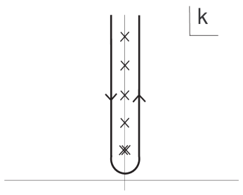
Figure 7: Contour for the integration in (A.21). It surrounds a double pole at $k=i$ and single poles at $k=2i,3i,\ldots$.

The result of the integration along the contour in Figure 7 is

$$\hat{G}_{c}^{(\bar{X})}(X_{1},X_{2};\theta)=\int_{-\infty}^{\infty}{dk\over 2\pi}{i(k+i)\over(2k+i)(k-i)}e^{-ik\bar{X}}{\sinh k(\pi-\theta)\over\sin\theta\sinh k\pi}$$

$$\qquad=\frac{1}{2\sin\theta}\frac{2\pi i}{2\pi}\sum_{n=2}^{\infty}e^{n\overline{X}}{n+1\over(2n+1)(n-1)}\frac{1}{\pi}\left(e^{-in\theta}-e^{in\theta}\right)$$

$$\qquad\quad+\frac{1}{2\sin\theta}\frac{2\pi i}{2\pi}{(-i)\over\pi}\partial_{k}\left\{{k+i\over 2k+i}e^{-ik\bar{X}}(e^{k\pi-k\theta}-e^{-k\pi+k\theta})\right\}\Big{|}_{k=i}$$ (A.21)

$$\qquad={1\over 12\pi\sin\theta}\Bigg{[}-ie^{(-\bar{X}+i\theta)/2}\log{1+e^{(\bar{X}-i\theta)/2}\over 1-e^{(\bar{X}-i\theta)/2}}+ie^{-(\bar{X}+i\theta)/2}\log{1+e^{(\bar{X}+i\theta)/2}\over 1-e^{(\bar{X}+i\theta)/2}}$$

$$\qquad\qquad\qquad-4ie^{\bar{X}-i\theta}\log(1-e^{\bar{X}-i\theta})+4ie^{\bar{X}+i\theta}\log(1-e^{\bar{X}+i\theta})+\frac{2}{3}ie^{\bar{X}-i\theta}-\frac{2}{3}ie^{\bar{X}+i\theta}\Bigg{]}$$

$$\qquad\quad+\frac{1}{2\pi\sin\theta}\left[-\frac{i}{9}e^{\bar{X}}(e^{-i\theta}-e^{i\theta})-\frac{2}{3}(-i\bar{X}+\pi-\theta)e^{\bar{X}-i\theta}+\frac{2}{3}(-i\bar{X}-\pi+\theta)e^{\bar{X}+i\theta}\right]$$

The bound state contribution to the correlator is

$$\hat{G}_{B}(X_{1},X_{2};\theta)=u_{B}(X_{1})u_{B}(X_{2})G_{B}(\theta)={2\over 3}e^{\bar{X}}{\cos\theta\over\sin\theta}\left(1-{\theta\over\pi}\right),$$ (A.22)

which also depends on $\bar{X}$. The coefficient 2/3 in (A.22) comes from the normalization of the bound state wave function $u_{B}(X)=\sqrt{2\over 3}a(X)$.

We add the continuum contribution (A.21) and the bound state contribution (A.22), and perform the analytic continuation (2.15) to the FRW region to get the $\bar{T}$ -dependent part of the rescaled Green’s function $\hat{G}^{(\bar{T})}(T_{1},T_{2};R)$. The $\bar{T}$ dependent part of the correlator $\langle\chi(T,0)\chi(T^{\prime},R)\rangle^{(\bar{T})}$ is related to the rescaled Green’s function we have calculated by

$$\langle\chi(T,0)\chi(T^{\prime},R)\rangle^{(\bar{T})}={\hat{G}^{(\bar{T})}(X_{1},X_{2};\theta)\over a(T_{1})a(T_{2})}$$

$$=-{2\over 3}i+{Re^{R}\over 3\pi\sinh R}+{e^{-\bar{T}}\over 12\pi\sinh R}\Bigg{[}ie^{-(\bar{T}+R)/2}\log{1+ie^{(\bar{T}+R)/2}\over 1-ie^{(\bar{T}+R)/2}}-ie^{-(\bar{T}-R)/2}\log{1+ie^{(\bar{T}-R)/2}\over 1-ie^{(\bar{T}-R)/2}}$$

$$\hskip 71.13188pt+4e^{(\bar{T}+R)}\log(1+e^{-(\bar{T}+R)})-4e^{(\bar{T}-R)}\log(1+e^{(\bar{T}-R)})+4\bar{T}e^{(\bar{T}-R)}\Bigg{]}$$ (A.23)

where the first two terms in the right hand side do not decay in the large $R$ limit, but rest of the terms do.

We shall make a technical comment here. The sum of the double pole contribution and the bound state contribution, whose Euclidean expressions are given by the last line of (A.21) and by (A.22), respectively, is

$$\langle\chi(T_{1},0)\chi(T_{2},R)\rangle^{(\bar{T})}_{\rm\scriptsize doublepole}+\langle\chi(T_{1},0)\chi(T_{2},R)\rangle^{(\bar{T})}_{B}=\frac{1}{\pi}(\frac{1}{9}-\frac{2}{3}\pi i-\frac{2}{3}\bar{T}),$$ (A.24)

and contains only constants and terms linear in $\bar{T}$. These terms vanish when we take derivatives of the correlator with respect to both points, so they do not affect physical quantities. We might call these terms “pure gauge.” Up to the pure gauge terms, we can say that the correlator is given solely by the contributions from the single poles (at $k=2i,3i,\ldots$). In fact, that is equivalent to solving for the correlator as an expansion in the spherical harmonics on $S^{3}$ (rather than in the eigenmodes of $[-\partial_{X}^{2}+U(X)]$), leaving out the zero-angular momentum mode on $S^{3}$.

The $\delta T=T_{1}-T_{2}$ dependent part $\langle\chi(T_{1},0)\chi(T_{2},R)\rangle^{(\delta T)}$, which might be called the “flat space piece,” is computed from the first term of (A.17). We get

$$\langle\chi(T_{1},0)\chi(T_{2},R)\rangle^{(\delta T)}=-{1\over 2\pi}{e^{-\bar{T}}\over\cosh\delta T-\cosh R},$$ (A.25)

for any CDL background. This is simply the usual flat-space correlator for a massless field, written in our coordinate system.

A.2.2 Large separation behavior

Let us study the large distance behavior of the correlator.

We have obtained the correlator as a function of $R$, taking one point to be at the origin of the hyperboloid $R=0$. When the two points are at general positions, the correlator is a function of the geodesic distance $\ell$, and is given by replacing $R$ with $\ell$ in the expressions that we have obtained. The geodesic distance $\ell$ between the two points on ${\cal H}_{3}$ located at $(R_{1},0)$ and $(R_{2},\alpha)$, where $\alpha$ is an angle in $S^{2}$, is given by

$$\cosh\ell=\cosh R_{1}\cosh R_{2}-\sinh R_{1}\sinh R_{2}\cos\alpha.$$ (A.26)

This relation can be obtained most easily by considering the inner product in the embedding space. In the limit of large separation, (A.26) reduces to

$$\ell\sim R_{1}+R_{2}+\log(1-\cos\alpha).$$ (A.27)

We take the late time limit as well as the large distance limit. Namely, we first take the $\bar{T}+\ell\to\infty$ limit and drop the terms with positive powers of $e^{-(\bar{T}+\ell)}$. The rest of the terms are given as an expansion in powers of $e^{\bar{T}-\ell}$.

Let us examine the large distance behavior of the correlator $\langle\chi\chi\rangle^{(\bar{T})}$, given in (A.23), in the large distance limit. We will write $\ell$ in place of $R$. We will ignore the pure gauge terms. As we mentioned, there is a piece in $\langle\chi\chi\rangle^{(\bar{T})}$ that does not decay at large distance. We shall call it $G_{2}$,

$$G_{2}={\ell e^{\ell}\over 3\pi\sinh\ell}.$$ (A.28)

This grows linearly with $\ell$, and in terms of the coordinates, its asymptotic form is

$$G_{2}\sim R_{1}+R_{2}+\log(1-\cos\alpha).$$ (A.29)

The the first two terms, $R_{1}$ and $R_{2}$, do not affect physical quantities because they disappear when we take derivatives with respect to the locations of both points. The last term, however, is physical. This piece represents a correlation which is independent of the radial position. Its interpretation is discussed further in the main text.

To find the subleading terms, we note that the flat space piece $\langle\chi\chi\rangle^{(\delta T)}$ in (A.25) yields $e^{-\bar{T}-R}/\pi$ when expanded in the large $R$ limit. This term is independent of $\delta T$, and precisely cancels the order $e^{-R}$ piece in $\langle\chi\chi\rangle^{(\bar{T})}$. We call $G_{1}$ the sum of the piece of $\langle\chi\chi\rangle^{(\bar{T})}$ apart from $G_{2}$ and $e^{-\bar{T}-R}/\pi$ from $\langle\chi\chi\rangle^{(\delta T)}$,

$$G_{1}=\frac{1}{12\pi}e^{-(\bar{T}+\ell)}\left\{-\frac{2}{3}e^{\bar{T}-\ell}+O(e^{2(\bar{T}-\ell)})-\pi e^{-(\bar{T}+\ell)/2}+O(e^{-2(\bar{T}+\ell)})\right\}.$$ (A.30)

This is an expansion in powers of $e^{\bar{T}-\ell}$ and of $e^{-(\bar{T}+\ell)}$. Higher orders of the expansions are indicated by $O(e^{2(\bar{T}-\ell)})$ and $O(e^{-2(\bar{T}+\ell)})$. In the limit of our interest, we ignore the last two terms of (A.30) which have positive powers of $e^{-(\bar{T}+R)}$. The leading term, which is the first term of (A.30), goes as $e^{-2\ell}$. We will call it the “dimension 2 piece.”

A.2.3 Asymptotic behavior and the poles of ${\cal R}(k)$

Each term in the series in (A.30) can be interpreted as arising from the poles of ${\cal R}(k)G_{k}(\theta)$. We shall give an alternative derivation of the asymptotic behavior (A.30).

The Euclidean expression for the correlation function ($\bar{X}$ dependent part) is

$$\langle\chi(X_{1},0)\chi(X_{2},\theta)\rangle^{(\bar{X})}=e^{-\bar{X}}\oint_{C}{dk\over 2\pi}{\cal R}(k)e^{-ik\bar{X}}{\sinh k(\pi-\theta)\over\sin\theta\sinh k\pi}$$ (A.31)

where the contour $C$ surrounds the single poles at $k=2i,3i,\ldots$. This contour is depicted in the main text, section 3, figure 2 (a). As we have mentioned, we can define the correlator either as the sum over contributions from poles at $k=i,2i,\ldots$ plus the bound state contribution, or as the contributions from the single poles alone. We take the latter definition here.

We perform analytic continuation at this stage,

$$\langle\chi(T_{1},0)\chi(T_{2},R)\rangle^{(\bar{T})}=e^{-\bar{T}}\oint_{C}{dk\over 2\pi}{\cal R}(k)e^{-ik\bar{T}}{\left(e^{-ikR}-e^{ikR-2\pi k}\right)\over 2\sinh R\sinh k\pi}.$$ (A.32)

If $+\bar{T}<0$ and $R-\bar{T}>0$, the integral along the contour $C$ converges. In the region of interest $R+\bar{T}>0$, $R-\bar{T}>0$, the second term containing $e^{ik(R-\bar{T})}$ converges along $C$, but the first term containing $e^{-ik(R+\bar{T})}$ does not. The correct analytic continuation of the $e^{-ik(R+\bar{T})}$ term is given by the integration along a contour closed in the opposite direction, which is depicted in Figure 2 (b). The summation over the contributions from the poles takes the form of an expansion valid in the large $R$ limit.

The integration for the $e^{ik(R-\bar{T})}$ terms picks up the residues of the single poles at $k=2i,3i,\ldots$, and gives rise to terms of the form $e^{-\bar{T}}e^{-n(\bar{T}-R)}/\sinh R$ with $n=2,3,\ldots$. These terms are subleading compared to the most interesting terms; as explained in the main text, each term takes the form of the correlator in Euclidean AdS₃ with a given $m^{2}$, and thus has a definite dimension in the CFT.

The integration for the $e^{-ik(\bar{T}+R)}$ terms along the contour in Figure 2 (b) first picks up the contribution from the double pole at $k=i$. It is of the form

$${ie^{-\bar{T}}\over 2\pi\sinh R}\partial_{k}\left\{(k-i){\cal R}(k)e^{-ik(\bar{T}+R)}\right\}\Big{|}_{k=i}.$$ (A.33)

This pole yields the terms of interest, the term that linearly grows with $R$ and the $e^{-2R}$ term, plus pure gauge terms.

There are single poles at $k=0,-2i,-3i,\ldots$, and also at $k=-i/2$ from the pole of ${\cal R}(k)$. There is no pole at $k=-i$, because ${\cal R}(k)$ generically has a zero at $k=-i$, as we show in section A.3.

From the pole at $k=0$, we get

$${-ie^{-\bar{T}}\over 2\pi\sinh R}{\cal R}(k=0).$$ (A.34)

Here ${\cal R}(k=0)=-1$ generally, except for the perfectly reflectionless potential for which ${\cal R}(k)=0$ identically. (See e.g. [30].) The piece (A.34) is canceled by the $k=0$ pole contribution from the flat space piece,

$$e^{-\bar{T}}\int{dk\over 2\pi}e^{ik\delta T}{\left(e^{-ikR+k\pi}-e^{ikR-k\pi}\right)\over 2\sinh R\sinh k\pi}.$$ (A.35)

Note that though the sum of the two terms in the integrand is regular at $k=0$, each term separately has a pole. We pick up this pole, since we are closing the contour in the different direction for each term.

The rest of the contributions from the integral of the $e^{-ik(\bar{T}+R)}$ term are of the form $e^{-\bar{T}}e^{n(\bar{T}+R)}/\sinh R$ with negative $n$. These terms can be neglected in our limit.

A.3 Asymptotic behavior in the general CDL geometry

We have studied the large distance limit of the correlator for a particular background, and found a piece which linearly grows with $\ell$ and a ‘dimension 2’ piece which goes like $e^{-2\ell}$. We now show that this behavior is true for general CDL backgrounds. As we have mentioned, the asymptotic behavior is determined by the poles of the reflection coefficient ${\cal R}(k)$. In this subsection, we obtain ${\cal R}(k)$ for general thin-wall geometries, and show that the above asymptotic behavior is general. Then we argue that our statement about the asymptotic behavior is true for thick-wall cases as well.

A.3.1 Reflection coefficient for general thin-wall

We consider general thin-wall geometries, where the size of the critical bubble (size of the bubble at the moment of nucleation) and the de Sitter radius are arbitrary. The Euclidean geometry is a flat disc patched to an arbitrary portion of a sphere. The scale factor is

$$a(X)={e^{X-X_{0}}\over\cosh X_{0}}\ \ (X\leq X_{0}),\qquad a(X)={1\over\cosh X}\ \ (X\geq X_{0}),$$ (A.36)

where we have set the de Sitter radius to unity. The $X_{0}\to-\infty$ limit corresponds to the small critical bubble, so that the Euclidean geometry includes almost all of the de Sitter sphere. The $X_{0}\to+\infty$ limit corresponds to the case where the Euclidean geometry includes only a tiny piece of the de Sitter sphere. The Green’s function can be calculated as in section A.1, A.2. The potential $U(X)=a^{\prime\prime}/a$, is given by

$$U(X)=1-{2\over\cosh^{2}X}\Theta(X-X_{0})-{e^{X_{0}}\over\cosh X_{0}}\delta(X-X_{0}).$$ (A.37)

To find the reflection coefficient, it is useful to note that the potential of the form $U(X)=a^{\prime\prime}/a$ can be embedded in supersymmetric quantum mechanics. (See [31] for a review on supersymmetric quantum mechanics.) The potential can be written as

$$U(X)=(W^{\prime})^{2}+W^{\prime\prime}$$ (A.38)

with $W=\log a$. We define the partner potential $\tilde{U}(X)$ by

$$\tilde{U}(X)=(W^{\prime})^{2}-W^{\prime\prime}.$$ (A.39)

The Schrödinger operator $(-\partial_{X}^{2}+U)$ for the original potential is written as $(\partial_{X}+W^{\prime})(-\partial_{X}+W^{\prime})$, and that for the partner potential is written as $(-\partial_{X}+W^{\prime})(\partial_{X}+W^{\prime})$. The wave function $u_{k}$ for $U(X)$ is related to the one $\tilde{u}_{k}$ for $\tilde{U}(X)$ with the same energy eigenvalue by the supersymmetry transformation $\tilde{u}_{k}=(-\partial_{X}+W^{\prime})u_{k}$. There is a one to one correspondence of the states except for the zero energy ground state $u_{B}=a(X)$ for $U(X)$, which is annihilated by the transformation $(-\partial_{X}+W^{\prime})u_{B}=0$.

The partner potential is flat either for the flat space potential $U(X)=1$, or for the sphere (de Sitter) potential $U(X)=1-2/\cosh^{2}X$. Thus, $\tilde{U}(X)$ for the thin-wall case is just a repulsive delta function at $X=X_{0}$:

$$\tilde{U}(X)=1+{e^{X_{0}}\over\cosh X_{0}}\delta(X-X_{0}).$$ (A.40)

The reflection coefficient $\tilde{{\cal R}}(k)$ for $\tilde{U}(X)$ is obtained by matching the plane waves on the two sides,

$$\tilde{{\cal R}}(k)={-ie^{2ikX_{0}}\over(e^{-2X_{0}}+1)k+i}.$$ (A.41)

Since the potential is repulsive, there is no bound state, and ${\cal R}(k)$ does not have a pole in the upper half $k$ plane.

Reflection and transmission coefficients for the original potential, ${\cal R}(k)$ and ${\cal T}(k)$, are defined in (A.6). Those for the partner potential $\tilde{{\cal R}}(k)$ and $\tilde{T}(k)$ are defined similarly from the asymptotic form of $\tilde{u}_{k}$. Applying the supersymmetry transformation to the asymptotic form of $u_{k}$, we get the relation

$$\tilde{{\cal R}}(k)={ik+W^{\prime}_{-}\over-ik+W^{\prime}_{-}}{\cal R}(k),\quad\tilde{T}(k)={-ik+W^{\prime}_{+}\over-ik+W^{\prime}_{-}}{\cal T}(k),$$ (A.42)

where $W^{\prime}_{\pm}=W^{\prime}(\pm\infty)$. Since the scale factor $a(X)$ behaves as $a(X)\propto e^{\pm X}$ for $X\to\mp\infty$, we always have $W^{\prime}_{\pm}=\mp 1$, and

$${\cal R}(k)=-{k+i\over k-i}\tilde{{\cal R}}(k),\quad{\cal T}(k)={k+i\over k-i}\tilde{T}(k).$$ (A.43)

From (A.41), we get

$${\cal R}(k)={i(k+i)e^{2ikX_{0}}\over(k-i)((e^{-2X_{0}}+1)k+i)}.$$ (A.44)

As we mentioned in section A.2, the bound state pole at $k=i$ is responsible for the leading terms in the large distance limit that we are interested in. We found here that there is no other poles than at $k=i$ in the upper half plane. In the lower half plane, there is a pole at $k=-(e^{-2X_{0}}+1)^{-1}i\equiv ai$ and a zero at $k=-i$. The pole is located between $k=0$ and $k=-i$ on the imaginary axis (in the half sphere example, at $k=-i/2$). This pole gives rise to the term $e^{-a({\bar{T}+R})}$, which can be neglected since we take the $\bar{T}+R\to\infty$ limit first.

The above discussion can be also applied to thick-wall cases. The potential is of the supersymmetric form. The partner potential is generally repulsive, since

$$\tilde{U}(X)=-{a^{\prime\prime}\over a}+2\left({a^{\prime}\over a}\right)^{2}={3\over 2}\left(\Phi^{\prime}\right)^{2}+1\geq 1$$ (A.45)

as we see from the Euclidean FRW equations (2.12). Thus, the partner potential will not have a bound state, and the reflection coefficient $\tilde{{\cal R}}(k)$ will not have a pole in the upper half plane. The reflection coefficient for the original potential ${\cal R}(k)$ is still related to $\tilde{{\cal R}}(k)$ by (A.43), since this relation was derived using only the asymptotic form of $a(X)$. This suggests that ${\cal R}(k)$ has only one pole in the upper half plane at $k=i$, and that the asymptotic behavior of the correlator that we found in section A.2 is true in general.

A.4 Scalar with mass in the false vacuum

So far, we have been considering a massless scalar, but we do not expect it to be present in the realistic situations. The “moduli field” $\Phi$ might be massless in the true vacuum, but it should be stabilized in the false vacuum.

To understand the behavior of scalars which have mass in the false vacuum, we shall study a simplified model. We consider a scalar which is massless in the flat space, and has infinite mass in the de Sitter space. Infinite mass makes the potential infinitely high. Wave function cannot penetrate into the de Sitter region, and the reflection coefficient is ${\cal R}(k)=-e^{2ikX_{0}}$, where the real number $X_{0}$ is the position of the domain wall as before. There is no bound state.

The correlation function is calculated from (A.17) and is given by

$$\langle\chi(T_{1},0)\chi(T_{2},R)\rangle=-e^{2X_{0}}\cosh^{2}X_{0}{e^{-\bar{T}}\over 2\pi}\left({1\over\cosh(\bar{T}-2X_{0})+\cosh R}+{1\over\cosh\delta T-\cosh R}\right),$$ (A.46)

where the factors outside the bracket are due to the rescaling by $a^{-1}(T_{1})a^{-1}(T_{2})$ to get the correlator of the physical field $\chi$. This correlator does not contain a piece which grows in the large distance. The leading term has dimension 2,

$$\langle\chi(T_{1},0)\chi(T_{2},R)\rangle\sim\cosh^{2}X_{0}{e^{-2R}\over\pi}.$$ (A.47)

When we have small but finite mass, there will be no linearly growing term, but still there will be non-normalizable correlations which scale like $e^{-\epsilon R}$. We expect this to happen as long as the bound state exists. Note that the effect of mass is to make the potential $U(X)$ shallow by adding a term $a(X)^{2}m^{2}$. Up to certain value of mass, there will be a bound state. The bound state energy should be in the range $0\leq(k^{2}+1)\leq 1$ (smaller than the asymptotic value of the potential); the bound state pole will be shifted from $k=i$ to $k=(1-\epsilon)i$, with $0\leq\epsilon\leq 1$.

The Euclidean correlator is expressed as an integral similar to the one for the massless case. Now the correlator is defined by an integral along the contour surrounding the poles at $k=i,2i,\ldots$, which goes between the poles at $k=i$ and $k=(1-\epsilon)i$. As in the massless case, the analytic continuation to Lorentzian is done by closing the contour for the term proportional to $e^{-ik(\bar{T}-R)}/\sinh R$ in the upper half plane, and the contour for the term proportional to $e^{-ik(\bar{T}+R)}/\sinh R$ in the lower half plane. The former integration picks up a contribution from the $k=i$ pole, which is now a single pole. It gives a dimension 2 piece. The latter integration has a contribution from the $k=(1-\epsilon)i$ pole. It gives a non-normalizable dimension $\epsilon$ piece, along with a subleading dimension $2+\epsilon$ piece.

It is instructive to consider the massless ($\epsilon\to 0$) limit. The sum of the $k=i$ and the $k=(1-\epsilon)i$ pole contributions is of the form

$${1\over\epsilon}\left({e^{-R}\over\sinh R}-{e^{(1-\epsilon)R}\over\sinh R}\right).$$ (A.48)

The $1/\epsilon$ factor reflects the fact that the residue at these poles are large because of the presence of the nearby pole. This factor has a relative minus sign for the two poles. In the $\epsilon\to 0$ limit, we recover the massless correlator, up to a divergent constant: The linearly growing term appears by taking the limit of $e^{\epsilon R}/\epsilon$. We also see that the $Re^{-2R}$ term in the massless correlator is a result of the coalescence of the dimension 2 piece and the dimension $(2+\epsilon)$ piece which have opposite signs.

Appendix B Graviton correlator in the CDL geometry

In this appendix we calculate graviton correlators in the CDL geometry. As in the scalar case, we get the correlator in the Euclidean CDL geometry and then analytically continue it to Lorentzian signature.

Our method explained in section B.1 and B.2 closely follows the one of Hawking, Hertog and Turok. See [32, 33] for more details. (See also [29, 34].) However, in section B.3, we reach a conclusion on the non-normalizable mode different from theirs.

B.1 General prescription

We consider the transverse traceless (TT) mode of graviton in the Euclidean CDL geometry. We define $h_{ab}$ to be the fluctuation of the metric around the CDL background $g_{ab}\to g_{ab}^{(CDL)}+h_{ab}$ which is TT on the $S^{3}$: $h^{a}_{a}=\nabla_{a}h^{a}_{b}=0$. We will use $a,b$ to denote the indices on $S^{3}$, or on ${\cal H}_{3}$ after analytic continuation.

The linearized equation of motion for the TT graviton (rescaled by $a(X)$) is

$$[-\partial^{2}_{X}+U(X)+2-\nabla^{2}](a(X)h_{ab}(X,\theta))=0,$$ (B.1)

where $U(X)=a^{\prime\prime}(X)/a(X)$. The eigenvalue of the Laplacian on $S^{3}$ for the TT tensor is $\nabla^{2}h_{ab}=[-l(l+2)+2]h_{ab}$ with $l=2,3,\ldots$. The equation of motion (B.1) is the same as the massless minimally coupled scalar equation, except that the angular momentum $l$ starts from 2 rather than 0.

We want to find the correlator $\hat{G}^{ab}{}_{a^{\prime}b^{\prime}}(X_{1},X_{2};\theta)=a(X_{1})a(X_{2})\langle h^{ab}(X_{1},\theta)h_{a^{\prime}b^{\prime}}(X_{2},0)\rangle$, which satisfies

$$[-\partial^{2}_{X_{1}}+U(X_{1})+2-\nabla^{2}]\hat{G}^{ab}{}_{a^{\prime}b^{\prime}}(X_{1},X_{2};\theta)=\delta(X_{1}-X_{2}){\delta(\theta)\over\sin^{2}\theta}\delta^{ab}{}_{a^{\prime}b^{\prime}}$$ (B.2)

where $\delta^{ab}{}_{a^{\prime}b^{\prime}}=\delta^{a}_{a^{\prime}}\delta^{b}_{b^{\prime}}+\delta^{a}_{b^{\prime}}\delta^{b}_{a^{\prime}}-{2\over 3}g^{ab}g_{a^{\prime}b^{\prime}}$.

The correlator can be expanded into harmonics on $S^{3}$,

$$\hat{G}^{ab}{}_{a^{\prime}b^{\prime}}(X_{1},X_{2};\theta)=\sum_{k=3i}^{+i\infty}\tilde{G}_{k}(X_{1},X_{2})W^{ab}_{(k)a^{\prime}b^{\prime}}(\theta)$$ (B.3)

where the sum is over $k=i(l+1)$ with $l=2,3,\ldots$. The bitensor (tensor with indices defined at two separate points) $W^{ab}_{(k)a^{\prime}b^{\prime}}(\theta)$ is an eigenfunction of the Laplacian

$$\nabla^{2}W^{ab}_{(k)a^{\prime}b^{\prime}}(\theta)=(k^{2}+3)W^{ab}_{(k)a^{\prime}b^{\prime}}(\theta),$$ (B.4)

and is regular over $S^{3}$ when $k$ takes the above values. It is a sum of products of tensor harmonics $q^{(k)}_{{\cal P}nm}{}^{ab}$ at two points ($\theta$ and 0); we fix $k$ and sum over other the quantum numbers ${\cal P}$, $m$, $n$ (parity and $S^{2}$ angular momenta),

$$W^{ab}_{(k)a^{\prime}b^{\prime}}(\theta)=\sum_{{\cal P}nm}q^{(k)}_{{\cal P}nm}{}^{ab}(\theta)q^{(k)}_{{\cal P}nm,}{}_{ab}(0)^{*},$$ (B.5)

where the tensor harmonics satisfy the eigenvalue equation $\nabla^{2}q^{(k)}_{{\cal P}nm}{}^{ab}=(k^{2}+3)q^{(k)}_{{\cal P}nm}{}^{ab}$, and the normalization $\int d\Omega q^{(k)}_{{\cal P}nm}{}^{ab}q^{(k^{\prime})*}_{{\cal P}^{\prime}n^{\prime}m^{\prime},}{}_{ab}=\delta^{kk^{\prime}}\delta_{{\cal P}{\cal P}^{\prime}}\delta_{nn^{\prime}}\delta_{mm^{\prime}}$. There is a completeness relation

$$\sum_{k=3i}^{+i\infty}W^{ab}_{(k)a^{\prime}b^{\prime}}(\theta)={\delta(\theta)\over\sin^{2}\theta}\delta^{ab}{}_{a^{\prime}b^{\prime}}.$$ (B.6)

The bitensor $W^{ab}_{(k)a^{\prime}b^{\prime}}(\theta)$ is invariant under the $SO(4)$ isometry, and is called the “maximally symmetric bitensor” [35, 36]. As in the scalar case, we will regard $k$ as a general complex number and obtain the correlator in an integral representation.

The function $\tilde{G}_{k}(X_{1},X_{2})$ satisfies

$$\left[-\partial_{X_{1}}^{2}+U(X_{1})-(k^{2}+1)\right]\tilde{G}_{k}(X_{1},X_{2})=\delta(X_{1}-X_{2}).$$ (B.7)

The solution can be written in terms of solutions of the homogeneous equation,

$$\tilde{G}_{k}(X_{1},X_{2})=\frac{1}{\Delta_{k}}\left[u_{k}^{R}(X_{1})u_{k}^{L}(X_{2})\Theta(X_{1}-X_{2})+u_{k}^{L}(X_{1})u_{k}^{R}(X_{2})\Theta(X_{2}-X_{1})\right]$$ (B.8)

where $u_{k}^{R}(X)$ and $u_{k}^{L}(X)$ are the solution of (B.7) without the delta function on the right hand side; $u_{k}^{R}(X)$ approaches $e^{ikX}$ as $X\to+\infty$, and $u_{k}^{L}(X)$ approaches $e^{-ikX}$ as $X\to-\infty$. $\Delta_{k}=-2ik$ is the Wronskian of $u_{k}^{L}$ and $u_{k}^{R}$. Since ${\rm Im}k>0$ here, (B.8) is regular away from the coincident point. When $X_{1},X_{2}\to-\infty$ and $X_{2}<X_{1}$, (B.8) becomes

$$\tilde{G}_{k}(X_{1},X_{2})={i\over 2k}\left(e^{ik\delta X}+{\cal R}(k)e^{-ik\bar{X}}\right),$$ (B.9)

where $\delta X=X_{1}-X_{2}$ and $\bar{X}=X_{1}+X_{2}$.

The graviton correlator in the Lorentzian CDL geometry is given by analytically continuing (B.3). We rewrite the sum (B.3) as an integral over $k$ before analytic continuation, and study the large distance behavior of the Lorentzian correlator using the contour deformation argument explained in A.2.3. The sum (B.3) can be written as

$$\hat{G}^{ab}{}_{a^{\prime}b^{\prime}}(X_{1},X_{2};\theta)=\oint_{\cal C}{dk\over 2i}\coth k\pi\,\tilde{G}_{k}(X_{1},X_{2})W^{ab}_{(k)a^{\prime}b^{\prime}}(\theta).$$ (B.10)

The factor $\coth k\pi$ gives rise to poles at integer multiple of $i$. The contour ${\cal C}$ is the one shown in Figure 2 (a) which surrounds $k=2i,3i,4i,\ldots$. In fact, for the tensor case, we do not have a pole at $k=2i$ since the bitensor is zero there, $W^{ab}_{(k=2i)a^{\prime}b^{\prime}}(\theta)=0$ [35, 33].

We perform analytic continuation to Lorentzian signature by $X\to T+{\pi\over 2}i$ and $\theta\to i\ell$, where $\ell$ is the geodesic distance on the hyperboloid.

$$\hat{G}^{ab}{}_{a^{\prime}b^{\prime}}(T_{1},T_{2};\ell)=\int{dk\over k\sinh k\pi}\,\left(e^{ik\delta T}+{\cal R}(k)e^{-ik\bar{T}}\right)W^{ab}_{(k)a^{\prime}b^{\prime}}(\ell).$$ (B.11)

As in the scalar case in A.2.3, for some terms, this integral along the coutour ${\cal C}$ does not converge in the region of interest $\ell+\bar{T}\to\infty$, $\ell-\bar{T}\to\infty$. The correct analytic continuation for these terms is given by closing the coutour in the other direction. Let us first find the explicit form the Lorentzian bitensor $W^{ab}_{(k)a^{\prime}b^{\prime}}(\ell)$ in the next subsection.

B.2 The Lorentzian bitensor

We first present the general expression in terms of the geodesic distance obtained in [35]. Then we evaluate it on the geodesic which connects two points near the boundary.

B.2.1 General form

The maximally symmetric bitensor $W^{ab}_{(k)a^{\prime}b^{\prime}}(\ell)$ has the following tensor structure,

$$W_{(k)}{}^{ab}{}_{a^{\prime}b^{\prime}}(\ell)=w_{k}^{(1)}(\ell)t^{(1)}{}^{ab}{}_{a^{\prime}b^{\prime}}+w_{k}^{(2)}(\ell)t^{(2)}{}^{ab}{}_{a^{\prime}b^{\prime}}+w_{k}^{(3)}(\ell)t^{(3)}{}^{ab}{}_{a^{\prime}b^{\prime}}$$ (B.12)

where the tensors $t^{(I)}{}^{ab}{}_{a^{\prime}b^{\prime}}$ ($I=1,2,3$) are independent of $k$, and are given by

$$t^{(1)}{}^{ab}{}_{a^{\prime}b^{\prime}} = (g^{ab}-3n^{a}n^{b})(g_{a^{\prime}b^{\prime}}-3n_{a^{\prime}}n_{b^{\prime}}),$$

$$t^{(2)}{}^{ab}{}_{a^{\prime}b^{\prime}} = C^{b}{}_{b^{\prime}}n^{a}n_{a^{\prime}}+C^{a}{}_{b^{\prime}}n^{b}n_{a^{\prime}}+C^{b}{}_{a^{\prime}}n^{a}n_{b^{\prime}}+C^{a}{}_{a^{\prime}}n^{b}n_{b^{\prime}}+4n^{a}n^{b}n_{a^{\prime}}n_{b^{\prime}},$$

$$t^{(3)}{}^{ab}{}_{a^{\prime}b^{\prime}} = C^{a}{}_{a^{\prime}}C^{b}{}_{b^{\prime}}+C^{b}{}_{a^{\prime}}C^{a}{}_{b^{\prime}}-2n^{a}g^{a^{\prime}b^{\prime}}n^{b}-2n_{a^{\prime}}g^{ab}n_{b^{\prime}}+6n^{a}n^{b}n_{a^{\prime}}n_{b^{\prime}}.$$ (B.13)

This is the general form which is traceless. It is known that the bitensor depends only on the following quantities [35, 36]: geodesic distance $\ell$, unit vectors $n_{a}$, $n_{a^{\prime}}$, which are tangent to the geodesic at the point $x$ and $x^{\prime}$ (vectors or tensors with unprimed (primed) indices are the ones defined at the point $x$ ($x^{\prime}$); $n_{a}$ and $n_{a^{\prime}}$ are defined to be pointing away from the other point), metrics at each point, and an operator $C_{ab^{\prime}}$ which parallel transports a vector from one point to the other along the geodesic.

The coefficient functions $w^{(I)}_{k}$ depend only on the geodesic distance. They are determined by the transversality condition and the eigenvalue equation for the Laplacian on the hyperboloid $\nabla^{2}_{H}W^{ab}_{(k)a^{\prime}b^{\prime}}=-(k^{2}+3)W^{ab}_{(k)a^{\prime}b^{\prime}}$:

$$w_{k}^{(1)}(\ell) = \frac{\sinh^{-5}\ell}{4\pi^{2}(k^{2}+1)}\Bigg{\{}\frac{\sin k\ell}{k}\left(3+(k^{2}+4)\sinh^{2}\ell-k^{2}(k^{2}+1)\sinh^{4}\ell\right)$$

$$~{}~{}~{}~{}-\cos k\ell\left(3/2+(k^{2}+1)\sinh^{2}\ell\right)\sinh 2\ell\Bigg{\}}$$

$$w_{k}^{(2)}(\ell) = \frac{\sinh^{-5}\ell}{4\pi^{2}(k^{2}+1)}\Bigg{\{}\frac{\sin k\ell}{k}\left(3+12\cosh\ell-3k^{2}(1+2\cosh\ell)\sinh^{2}\ell+k^{2}(k^{2}+1)\sinh^{4}\ell\right)$$

$$~{}~{}~{}~{}+\cos k\ell\left(-12-3\cosh\ell+2(k^{2}-2)\sinh^{2}\ell+2(k^{2}+1)\cosh\ell\sinh^{2}\ell\right)\sinh\ell\Bigg{\}}$$

$$w_{k}^{(3)}(\ell) = \frac{\sinh^{-5}\ell}{4\pi^{2}(k^{2}+1)}\Bigg{\{}\frac{\sin k\ell}{k}\left(3-3k^{2}\sinh^{2}\ell+k^{2}(k^{2}+1)\sinh^{4}\ell\right)$$ (B.14)

$$~{}~{}~{}~{}+\cos k\ell\left(-3/2+(k^{2}+1)\sinh^{2}\ell\right)\sinh 2\ell\Bigg{\}}$$

B.2.2 Behavior near the boundary

Let us write the bitensor explicitly when the two points are near the boundary (spatial infinity). We will use the Poincaré coordinate on the hyperboloid

$$ds^{2}={1\over z^{2}}(dz^{2}+dx^{2}+dy^{2}),$$ (B.15)

where the boundary is at $z=0$, and is parametrized by $x$ and $y$. We consider two points at $(x,y,z)$ and $(-x,-y,z)$; we will take the $z\to 0$ limit eventually.

We can obtain the geometric quantities that appear in the bitensor by recalling that the geodesic which connects two points on the boundary is a half circle in the Poincare coordinate. The unit tangent vector $n_{a}$ at $(x,y,z)$ is

$$\pmatrix{n_{z}\cr n_{x}\cr n_{y}}={\sqrt{x^{2}+y^{2}}\over z\sqrt{x^{2}+y^{2}+z^{2}}}\pmatrix{-1\cr{x\over x^{2}+y^{2}}z\cr{y\over x^{2}+y^{2}}z},$$ (B.16)

and $n_{a^{\prime}}$ at $(-x,-y,z)$ is given by replacing $x$ and $y$ with $-x$ and $-y$ in the above equation.

The parallel transport operator $C_{ab^{\prime}}$ transforms the tangent vector at one point to the one at the other point, $n_{a}=-C_{a}{}^{b^{\prime}}n_{b^{\prime}}$, and it preserves the norm of a vector. In fact, in the present case where the $z$ coordinate of the two points are equal, $C_{ab^{\prime}}$ is a rotation matrix, and we find

$$\pmatrix{C_{z}{}^{z}&C_{z}{}^{x}&C_{z}{}^{y}\cr C_{x}{}^{z}&C_{x}{}^{x}&C_{x}{}^{y}\cr C_{y}{}^{z}&C_{y}{}^{x}&C_{y}{}^{y}\cr}={1\over x^{2}+y^{2}+z^{2}}\pmatrix{-x^{2}-y^{2}+z^{2}&-2zx&-2zy\cr 2zx&-x^{2}+y^{2}+z^{2}&-2xy\cr 2zy&-2xy&x^{2}-y^{2}+z^{2}}$$ (B.17)

Geodesic distance between $(x,y,z)$ and $(-x,-y,z)$ is

$$\ell=\int ds\sqrt{g_{ab}{dx^{a}\over ds}{dx^{b}\over ds}}=2\log{\sqrt{x^{2}+y^{2}+z^{2}}+\sqrt{x^{2}+y^{2}}\over z}.$$ (B.18)

We substitute these expressions into the bitensor and obtain the correlator (B.11) in an expansion in $z$.

B.3 Large distance behavior of the correlator

We study the large distance, late time behavior of the correlator (B.11) in exactly the same way as we did for the scalar in section A.2.3. We will concentrate on the piece which depend on $\bar{T}$ (the second term of (B.11)).

First, note that the bitensor (B.14) consists of pieces proportional to $e^{-ik\ell}$ and those proportional to $e^{ik\ell}$; the coefficient functions $w^{(I)}_{k}$ are of the form $w^{(I)}_{k}=\hat{w}_{k}^{(I)}e^{-ik\ell}+\tilde{w}_{k}^{(I)}e^{ik\ell}$, and $\hat{w}^{(I)}_{k}$ and $\tilde{w}_{k}^{(I)}$ goes like $e^{-\ell}$ in the large $\ell$ limit. Also note that the tensor structures $t^{(I)}{}^{ab}{}_{a^{\prime}b^{\prime}}$ starts from order 1 terms.

As in the scalar case, the integration for the terms involving $e^{-ik(\bar{T}-\ell)}$ is performed along the contour in the Figure 2 (a) which surrounds the single poles at $k=3i,4i,\ldots$. (No pole at $k=2i$ for graviton case.) For the terms involving $e^{ik(\bar{T}+\ell)}$, the integration is done along the contour in Figure 2 (b); it surrounds the double pole at $k=i$, and single poles at $k=0$ and in the lower half plane. The contribution from the $k=i$ double pole in the latter integral yields the terms that we are interested in. The rest of the terms are subleading for the reason we explained in section A.2.3.

The contribution from the $k=i$ double pole takes the form

$$\langle h^{ab}h_{a^{\prime}b^{\prime}}\rangle_{(k=i)}=ce^{-\bar{T}}\sum_{I=1}^{3}\partial_{k}\left((k-i){\cal R}(k){e^{-ik\bar{T}}\over k}\hat{w}^{(I)}_{k}(\ell)e^{-ik\ell}\right)\bigg{|}_{k=i}t^{(I)}{}^{ab}{}_{a^{\prime}b^{\prime}}$$ (B.19)

where $c$ is a constant, and the $e^{-\bar{T}}$ factor is due to the rescaling to get the physical correlator.

B.3.1 Dimension 0 piece

The leading term of the correlator grows linearly with the geodesic distance $\ell$. This term arises when the $k$-derivative in (B.19) hits $e^{-ik\ell}$.

The tensor structure of this piece is given by the leading term of $\sum_{I}\hat{w}_{(k=i)}^{(I)}t^{(I)ab}{}_{a^{\prime}b^{\prime}}$. Substituting (B.14) into $\hat{w}_{(k=i)}^{(I)}$, and (B.13), (B.16), (B.17) into $t^{(I)ab}{}_{a^{\prime}b^{\prime}}$, we find that the tensor structure of the dimension 0 piece is as follows. If the correlator has at least one $z$ index, it is of order $O(z^{2})$; in other words, the order 1 correlator has all its indices along the boundary directions,

$$\langle h^{ij}h_{i^{\prime}j^{\prime}}\rangle_{(0)}=c_{0}\ell\,t{}^{ij}{}_{i^{\prime}j^{\prime}}$$ (B.20)

where $c_{0}$ is a constant, and $i,j=1,2$ denotes the indices along the 2 dimensional plane along the boundary. The tensor $t{}^{ij}{}_{i^{\prime}j^{\prime}}$ is traceless in the 2-D sense, $t{}^{i}{}_{ii^{\prime}j^{\prime}}=0$, since the correlator is traceless on the hyperboloid by construction, and the radial component is zero to this order. Explicit form when the two points are at $(x,y,z)$ and $(-x,-y,z)$ is

$$t_{x}{}^{x}{}_{x}{}^{x}=-t_{x}{}^{x}{}_{y}{}^{y}=-t_{x}{}^{y}{}_{x}{}^{y}=-{(x^{4}-6x^{2}y^{2}+y^{4})\over(x^{2}+y^{2})^{2}},\quad t_{x}{}^{x}{}_{x}{}^{y}=-t_{y}{}^{y}{}_{x}{}^{y}=-{4(x^{2}-y^{2})xy\over(x^{2}+y^{2})^{2}}.$$ (B.21)

The geodesic distance is given by $\ell=2\log{2\sqrt{x^{2}+y^{2}}\over z}$ to the leading order.

Let us calculate a gauge invariant quantity associated with this correlator. We find that the 2-D scalar curvature of the graviton fluctuation has finite ($z$-independent) correlation when the two points approach the boundary. The scalar curvature is given by $C=h_{i}{}^{i}{}_{;j}{}^{;j}-h_{i}{}^{j}{}_{;j}{}^{;i}-R_{i}{}^{k}h_{j}{}^{i}$, where the semi-colon denotes the covariant derivative in the background 2-D space, and $R_{i}{}^{j}$ is the 2-D Ricci tensor of the background. The first and the third terms are zero, since the fluctuation is traceless and the background is flat. From (B.20), we get

$$\langle C(x_{1})C(x_{2})\rangle=\partial^{i}\partial_{j}\partial^{i^{\prime}}\partial_{j^{\prime}}\langle h_{i}{}^{j}(x_{1})h_{i^{\prime}}{}^{j^{\prime}}(x_{2})\rangle_{(0)}={2c_{0}\over\left\{(x^{i}_{1}-x^{i}_{2})(x^{i}_{1}-x^{i}_{2})\right\}^{2}}.$$ (B.22)

The 2-D curvature behaves as a dimension 2 field.

B.3.2 Transverse-traceless (TT) dimension 2 piece

Let us now study the subleading terms. Let us first look for the terms which do not contain the linear factor in $\ell$.

We ignore the pure gauge piece which does not contribute to the physical quantities, as we have ignored the constant term in the scalar case. Note that the bitensor $W_{(k=i)}^{ab}{}_{a^{\prime}b^{\prime}}$ evaluated at $k=i$ is a pure gauge. It is known that the tensor harmonics on ${\cal H}_{3}$ at $k=i$, which satisfy $\nabla^{2}_{H}q_{ab}=-2q_{ab}$, can be written in the form of a gauge transformation $q_{ab}=\nabla_{a}v_{b}+\nabla_{b}v_{a}$ with a gauge parameter $v_{a}$ satisfying $\nabla^{2}_{H}v_{a}=2v_{a}$ [34, 33]. Thus, we can add a term proportional (by an $\ell$-independent factor) $W_{(k=i)}^{ab}{}_{a^{\prime}b^{\prime}}=\sum_{I}(\hat{w}^{(I)}_{k=i}e^{\ell}+\tilde{w}^{(I)}_{k=i}e^{-\ell})t^{(I)}{}^{ab}{}_{a^{\prime}b^{\prime}}$ to the correlator without affecting the physical properties.

In the literature [34, 33], it is stated that the “supercurvature mode” (non-normalizable mode) is absent for tensor perturbations. It seems that the whole contribution from the $k=i$ pole is neglected assuming it is pure gauge, contrary to our discussion here. If we start from the Euclidean prescription, we find no reason to neglect the $k=i$ pole contributions except for the pure gauge term mentioned above. We are finding important physical pieces from this pole.

In the double pole contribution (B.19), there is a term where the $k$-derivative hits $(k-i){\cal R}(k)/k$. This term is proportional to $\sum_{I}\hat{w}^{(I)}_{k=i}e^{\ell}t^{(I)}{}^{ab}{}_{a^{\prime}b^{\prime}}$ and is of order 1. Up to pure gauge, this term can be written in the form $\sum_{I}\tilde{w}^{(I)}_{k=i}e^{-\ell}t^{(I)}{}^{ab}{}_{a^{\prime}b^{\prime}}$, which is of order $z^{4}$ (which corresponds to dimension 2),

$$\langle h^{ij}h_{i^{\prime}j^{\prime}}\rangle_{(2)}={c_{2}z^{4}\over(x^{2}+y^{2})^{2}}t{}^{ij}{}_{i^{\prime}j^{\prime}},$$ (B.23)

where $c_{2}$ is a constant and the tensor $t^{ij}{}_{i^{\prime}j^{\prime}}$ is given by (B.21). The correlator $\langle h^{ij}h_{i^{\prime}j^{\prime}}\rangle_{(2)}$ is traceless in 2-D, and is also transverse in the 2-D space,

$$\partial_{i}\langle h^{ij}h_{i^{\prime}j^{\prime}}\rangle_{(2)}=0,$$ (B.24)

as we can check explicitly. Or more simply, we can write the correlator in the complex coordinate $u=x+iy$, and check that it is holomorphic $\langle h^{uu}h^{uu}\rangle\sim 1/u^{4}$, $\langle h^{uu}h^{\bar{u}\bar{u}}\rangle=0$.

B.3.3 Non-TT dimension 2 piece

In the $k=i$ contribution (B.19), there is one more piece, which arises when the $k$-derivative hits the coefficient function $\hat{w}^{(I)}_{k}$. By subtracting the pure gauge, we can show that the leading term from this piece is of order $z^{4}$ (dimension 2). However, this dimension 2 piece has a tensor structure different from the above one, and is neither transverse nor traceless in the 2-D sense.

Also, as in the scalar case, the dimension 0 (logarithmic) term has subleading corrections and gives rise to the dimension 2 piece with the logarithmic prefactor. This piece is also non-TT in 2-D.

To interpret these terms, let us temporarily assume that the pole of ${\cal R}(k)$ is at a slightly shifted position $k=(1-\epsilon)i$. As we have discussed in section A.4 for the scalar case, we will have separate contributions from the single poles at $k=i$ and $k=(1-\epsilon)i$. The former is proportional to $\tilde{w}_{k}e^{ik\ell}t^{(I)}{}^{ab}{}_{a^{\prime}b^{\prime}}|_{k=i}$. This always has dimension 2 (after subtracting the pure gauge term), and is TT in 2-D. In the text, we identify this piece as a candidate for the energy-momentum tensor of the CFT. The contribution from the $k=(1-\epsilon)i$ pole is proportional to $\hat{w}_{k}e^{-ik\ell}t^{(I)}{}^{ab}{}_{a^{\prime}b^{\prime}}|_{k=i}$. This term yields pieces with dimension $\epsilon$ and $2+\epsilon$, which are non-TT in 2-D.

The non-TT dimension 2 piece in the massless graviton correlator that we found above is a consequence of merging of the poles. As in the scalar case, the dimension 2 piece and dimension $2+\epsilon$ piece have opposite signs, and in the massless limit $\epsilon\to 0$, they give rise to terms which involve the derivative of the bitensors with respect to $k$.

References

- [1] G. ’t Hooft, “Dimensional Reduction in Quantum Gravity” [arXiv:gr-qc/9310026]; L. Susskind, “The World as a Hologram,” J. Math. Phys. 36 (1995) 6377 [arXiv:hep-th/9409089];
- [2] R. Bousso, “The holographic principle,” Rev. Mod. Phys. 74 (2002) 825 [arXiv:hep-th/0203101].
- [3] J. M. Maldacena, “The Large N limit of superconformal field theories and supergravity,” Adv. Theor. Math. Phys. 2 (1998) 231, Int. J. Theor. Phys. 38 (1999) 1113 [arXiv:hep-th/9711200].
- [4] O. Aharony, S. S. Gubser, J. M. Maldacena, H. Ooguri and Y. Oz, “ Large N field theories, string theory and gravity,” Phys. Rept. 323 (2000) 183 [arXiv:hep-th/9905111].
- [5] R. Bousso and J. Polchinski, “Quantization of four-form fluxes and dynamical neutralization of the cosmological constant,” JHEP 0006 (2000) 006 [arXiv:hep-th/0004134]; L. Susskind, “The Anthropic Landscape of String Theory” [arXiv:hep-th/0302219].
- [6] S. Kachru, R. Kallosh, A. Linde and S. P. Trivedi, “De Sitter vacua in string theory,” Phys. Rev. D 68 (2003) 046005 [arXiv:hep-th/0301240]; M. R. Douglas, “The Statistics of string / M theory vacua,” JHEP 0305 (2003) 046 [arXiv:hep-th/0303194]; F. Denef and M. R. Douglas, “Distributions of flux vacua,” JHEP 0405 (2004) 072 [arXiv:hep-th/0404116].
- [7] A. Vilenkin, “Birth of inflationary universes,” Phys. Rev. D 27 (1983) 2848; P. J. Steinhardt, “Natural Inflation,” in The Very Early Universe, eds. G.W. Gibbons, S.W. Hawking, and S.T.C. Siklos, Cambridge University Press, 1983, p. 251. A. D. Linde, “Eternal Chaotic Inflation,” Mod. Phys. Lett. A 1 (1986) 81.
- [8] A. H. Guth, “Inflation and eternal inflation,” Phys. Rept. 333 (2000) 555 [arXiv:astro-ph/0002156].
- [9] S. R. Coleman and F. De Luccia, “Gravitational Effects On And Of Vacuum Decay,” Phys. Rev. D 21 (1980) 3305; B. Freivogel and L. Susskind, Phys. Rev. D 70 (2004) 126007 [arXiv:hep-th/0408133].
- [10] R. Bousso and B. Freivogel, Phys. Rev. D 73 (2006) 083507 [arXiv:hep-th/0511084].
- [11] A. Strominger, “The dS/CFT correspondence,” JHEP 0110 (2001) 034 [arXiv:hep-th/0106113].
- [12] L. Dyson, J. Lindesay and L. Susskind, “Is there really a de Sitter/CFT duality?” JHEP 0208 (2002) 045 [arXiv:hep-th/0202163].
- [13] J. B. Hartle and S. W. Hawking, “Wave Function of the Universe,” Phys. Rev. D 28 (1983) 2960.
- [14] H. L. Verlinde “Holography and compactification,” Nucl. Phys. B 580 (2000) 264 [arXiv:hep-th/9906182].
- [15] S. S. Gubser, “AdS/CFT and gravity,” Phys. Rev. D 63 (2001) 084017 [arXiv:hep-th/9912001];
- [16] S. Hawking, J. M. Maldacena and A. Strominger, “de Sitter entropy, quantum entanglement and AdS / CFT,” JHEP 0105 (2001) 001 [arXiv:hep-th/0002145].
- [17] M. Alishahiha, A. Karch, E. Silverstein and D. Tong, “The dS/dS correspondence,” AIP Conf. Proc. 743 (2005) 393 [arXiv:hep-th/0407125]; M. Alishahiha, A. Karch and E. Silverstein, “Hologravity,” JHEP 0506 (2005) 028 [arXiv:hep-th/0504056].
- [18] B. Freivogel, V. E. Hubeny, A. Maloney, R. Myers, M. Rangamani and S. Shenker, “Inflation in AdS/CFT,” JHEP 0603 (2006) 007 [arXiv:hep-th/0510046].
- [19] T. Hertog and G. T. Horowitz, “Towards a big crunch dual,” JHEP 0407 (2004) 073 [arXiv:hep-th/0406134]; T. Hertog and G. T. Horowitz, “Holographic description of AdS cosmologies,” JHEP 0504 (2005) 005 [arXiv:hep-th/0503071].
- [20] J. de Boer and S. N. Solodukhin, “A holographic reduction of Minkowski space-time,” Nucl. Phys. B 665 (2003) 545 [arXiv:hep-th/0303006].
- [21] L. Susskind and E. Witten, “The Holographic bound in anti-de Sitter space” [arXiv:hep-th/9805114].
- [22] A. W. Peet and J. Polchinski, “UV / IR relations in AdS dynamics,” Phys. Rev. D 59 (1999) 065011 [arXiv:hep-th/9809022].
- [23] B. S. DeWitt, “Quantum Theory of Gravity. I. The Canonical Theory,” Phys. Rev. 160 (1967) 1113; J. A. Wheeler, “Superspace and the Nature of Quantum Geometrodynamics,” in Battelle Rencontres: 1967, Lectures in Mathematical Physics, eds. C. M. DeWitt and J. A. Wheeler, W.A. Benjamin, 1968.
- [24] T. Banks, W. Fischler and L. Susskind, “Quantum Cosmology In (2+1)-Dimensions And (3+1)-Dimensions,” Nucl. Phys. B 262 (1985) 159.
- [25] T. Banks, “T C P, quantum gravity, the cosmological and all that…,” Nucl. Phys. B 249 (1985) 332.
- [26] A. M. Polyakov, “Quantum Geometry Of Bosonic Strings,” Phys. Lett. B 103 (1981) 207; A. Zamolodchikov and A. Zamolodchikov, “Conformal bootstrap in Liouville field theory,” in Cargese 1995, Low-dimensional applications of quantum field theory.
- [27] A. H. Guth and E. J. Weinberg, “Could the Universe have Recovered from a Slow First Order Phase Transition?” Nucl. Phys. B 212 (1983) 321.
- [28] S. Gratton and N. Turok, “Cosmological Perturbations from the No Boundary Euclidean Path Integral,” Phys. Rev. D 60 (1999) 123507 [arXiv:astro-ph/9902265].
- [29] M. Bucher, A. S. Goldhaber and N. Turok, “An open universe from inflation,” Phys. Rev. D 52 (1995) 3314 [arXiv:hep-ph/9411206]; M. Bucher and J. D. Cohn, “Primordial gravitational waves from open inflation,” Phys. Rev. D 55 (1997) 7461 [arXiv:astro-ph/9701117]; J. Garriga, X. Montes, M. Sasaki and T. Tanaka, “Spectrum of cosmological perturbations in the one bubble open universe,” Nucl. Phys. B 551 (1999) 317 [arXiv:astro-ph/9811257]; A. Linde, M. Sasaki and T. Tanaka, “CMB in Open Inflation,” Phys. Rev. D 59 (1999) 123522 [arXiv:astro-ph/9901135].
- [30] G. Barton, “Levinson’s theorem in one dimension: heuristics,” J. Phys. A 18 (1985) 479.
- [31] F. Cooper, A. Khare and U. Sukhatme, “Supersymmetry and Quantum Mechanics,” Phys. Rept. 251 (1995) 267 [arXiv:hep-th/9405029].
- [32] T. Hertog and N. Turok, “Gravity waves from instantons,” Phys. Rev. D 62 (2000) 083514 [arXiv:astro-ph/9903075].
- [33] S. W. Hawking, T. Hertog and N. Turok, “Gravitational waves in open de Sitter space,” Phys. Rev. D 62 (2000) 063502 [arXiv:hep-th/0003016].
- [34] T. Tanaka and M. Sasaki, “The spectrum of gravitational wave perturbations in the one bubble open inflationary universe,” Prog. Theor. Phys. 97 (1997) 243 [arXiv:astro-ph/9701053].
- [35] B. Allen, “Maximally symmetric spin two bitensors on and ,” Phys. Rev. D 51 (1995) 5491 [arXiv:gr-qc/9411023].
- [36] B. Allen and T. Jacobson, “Vector Two Point Functions In Maximally Symmetric Spaces,” Commun. Math. Phys. 106 (1986) 201.