hep–th/0606190

Supergravity and the jet quenching parameterin the presence of R-charge densities

Spyros D. Avramis^1,2 x andx Konstadinos Sfetsos²

${}^{1}\!$ Department of Physics, National Technical University of Athens,

15773, Athens, Greece

${}^{2}\!$ Department of Engineering Sciences, University of Patras,

26110 Patras, Greece

avramis@mail.cern.ch,   sfetsos@upatras.gr

Abstract

Following a recent proposal, we employ the AdS/CFT correspondence to compute the jet quenching parameter for ${\cal N}=4$ Yang–Mills theory at nonzero R-charge densities. Using as dual supergravity backgrounds non-extremal rotating branes, we find that the presence of the R-charges generically enhances the jet quenching phenomenon. However, at fixed temperature, this enhancement might or might not be a monotonically increasing function of the R-charge density and depends on the number of independent angular momenta describing the solution. We perform our analysis for the canonical as well as for the grand canonical ensemble which give qualitatively similar results.

1 Introduction and summary

There exists strong evidence from RHIC data that the hot, dense QCD plasma produced at the temperature range $T_{\rm c}<T<4T_{\rm c}$, where $T_{\rm c}$ is the crossover temperature, remains strongly coupled ($g^{2}N\simeq 10$) despite the partial deconfinement of color charges (see e.g. [2] for a review). As such, its behavior is similar to that of a nearly perfect fluid and its macroscopic properties admit an effective description in terms of hydrodynamics [3]. However, the hydrodynamic parameters characterizing the fluid are notoriously hard to compute using conventional approaches and, being of dynamical nature, they are not amenable to lattice calculations.

On the other hand, the fact that the theory is strongly coupled in the above temperature range suggests the use of nonperturbative gauge/gravity dualities for such computations. Unfortunately, such dualities do not apply to real QCD but rather to its supersymmetric generalizations, the prototype example being the AdS/CFT correspondence [4] relating Type IIB string theory on $AdS_{5}\times S^{5}$ to ${\cal N}=4$ SYM. Nevertheless, there is some hope that, in a strongly-coupled yet non-confining regime, some basic aspects of QCD dynamics may be captured by a supersymmetric theory possessing a gravity dual. This line of approach was employed in a series of works [5] for the calculation of transport coefficients which yielded the remarkable result that the ratio of shear viscosity to entropy density attains a universal value, close to the observed one, in any theory with a gravity dual [6] (see also [7]). Such encouraging results provide enough motivation for trying to apply, with the proper caution, gauge/gravity dualities in the study of phenomena related to the QCD plasma.

An interesting phenomenon in the above class is jet quenching, the energy loss of high–$p_{T}$ partons produced in heavy-ion collisions as they interact with the plasma before they fragment into hadrons [8, 9]. The “transport coefficient” characterizing the phenomenon is the jet quenching parameter $\hat{q}$, usually defined perturbatively as the average loss in four-momentum squared per mean free path. By analogy to high-energy scattering studied in the framework of eikonal approximations (see e.g. [9]), the problem of jet quenching can be formulated [10] in terms of Wilson loops in the adjoint representation. In such a context, $\hat{q}$ can be calculated according to the relation

$$\langle W^{A}(C)\rangle\ =\exp\left(-{1\over 4}\hat{q}L^{-}L^{2}\right)\ ,$$ (1.1)

where $W^{A}(C)$ is an adjoint Wilson loop on a rectangular contour $C$ with one lightlike and one spacelike side of lengths $L^{-}$ and $L$ respectively, with $L\ll L^{-}$.

The fact that Wilson loops of this type lend themselves to strong-coupling calculations via gauge/gravity dualities [12, 13, 14] motivated Liu, Rajagopal and Wiedemann [15] to postulate that the above relation may be taken as a nonperturbative operational definition of $\hat{q}$, and to calculate its value in ${\cal N}=4$ SYM according to AdS/CFT. At large $N$, one may take $\langle W^{A}(C)\rangle\simeq\langle W^{F}(C)\rangle^{2}$, where $W^{F}(C)$ is a fundamental Wilson loop, and use the AdS/CFT relation $\langle W^{F}(C)\rangle=\exp\left({\rm i}S[C]\right)$, where $S[C]$ is the Nambu-Goto action for a string propagating in the dual gravity background and whose endpoints trace the contour $C$. Noting that the exponent in (1.1) is real, the action $S[C]$ must be imaginary, i.e. the string configuration of interest must be spacelike. Writing $S[C]={\rm i}\tilde{S}[C]$, where $\tilde{S}[C]$ is real, we find that $\hat{q}$ is determined by

$$\frac{1}{8}\hat{q}L^{-}L^{2}=\tilde{S}[C]\ ,$$ (1.2)

in the limit of small $L$. The meaning of the above relation is that one should seek a solution of the string equations of motion with the string endpoints lying on the lightlike loop $C$ and, provided that the leading term in the small-$L$ expansion of its action is proportional to $L^{2}$, read off the coefficient $\hat{q}$ from (1.2).

Two other observables related to the phenomenon of energy loss in plasmas is the drag force exerted on a heavy quark as it travels through the plasma and the heavy-quark diffusion coefficient; in the context of AdS/CFT, these have been calculated in [16, 17] and [18] respectively while the first approach was further explored in [19, 20, 21].

The validity of the approach described above for the computation of $\hat{q}$ and its relation to the “drag force” approach to the study of parton energy loss has been a subject of much debate in the recent literature [22, 23, 24]. To begin, the two approaches are conceptually completely different as the proposal of [15] corresponds to a limiting case of a quark-antiquark string solution [25] whose action is required to be imaginary, while that of [16, 17] refers to a single-quark string solution with the whole computation based on the requirement that the action be real. In this respect, it is now quite clear [16, 23] that the two types of approach describe different physics, with the approach of [15] presumably best suited to light quarks and that of [16, 17] best suited to heavy quarks. Nevertheless, it is still argued [24] that the implicit limiting procedure employed in [15] is not valid and that the spacelike string used there does not dominate the path integral. Although such points will not be further discussed here, we must stress that the computations presented in this paper are valid provided that the proposal of [15] is on solid grounds.

Be that as it may, the value of $\hat{q}$ computed in [15] is of the correct order of magnitude, and the obvious question is how it is modified in more generalized settings, as done for example in [26] for certain non-conformal cases. In this paper we compute the jet quenching parameter, by means of the method outlined above, for the case of ${\cal N}=4$ SYM in the presence of nonzero R-charges. In section 2, we review the dual supergravity backgrounds, corresponding to non-extremal rotating D3-branes, and we concentrate on two cases with one or two equal nonzero angular momenta, for which we state the criteria for thermodynamic stability and the relations between the gauge-theory and supergravity parameters. In section 3, we compute exactly the jet quenching parameter $\hat{q}$ as a function of the thermodynamic parameters of the gauge theory, in both the canonical and grand canonical ensembles. Our main conclusion is that turning on nonzero R-charges generically enhances the jet quenching phenomenon, in a manner dependent on the number of non-vanishing equal angular momenta.

2 Non-extremal rotating branes

According to the AdS/CFT correspondence, ${\cal N}=4$ super Yang-Mills theory with $SU(N)$ gauge group is dual to a stack of $N$ extremal D3-branes. Introducing finite temperature corresponds to replacing the extremal branes by non-extremal ones [27], while introducing nonzero R-charges corresponds to generalizing the branes to rotating ones. This class of metrics has been found in full generality in [28] using previous results from [29]. They are characterized by the non-extremality parameter $\mu$ plus the rotation parameters $a_{i}$, $i=1,2,3$, which correspond to the three generators of the Cartan subalgebra of $SO(6)$ and are related to three chemical potentials (or R-charges) in the gauge theory. The most general non-extremal rotating D3-brane solution in the field-theory limit is given by [30]

$$ds^{2}=H^{-1/2}\left[-\left(1-{\mu^{4}\over r^{4}\Delta}\right)dt^{2}+dx^{2}+dy^{2}+dz^{2}\right]+H^{1/2}{r^{6}\Delta\over f}\ dr^{2}$$

$$\,+\>\>H^{1/2}\Bigg{[}r^{2}\Delta_{1}d\theta^{2}+r^{2}\Delta_{2}\cos^{2}\theta d\psi^{2}+2(a_{2}^{2}-a_{3}^{2})\cos\theta\sin\theta\cos\psi\sin\psi d\theta d\psi$$ (2.1)

$$\,+\>\>(r^{2}+a_{1}^{2})\sin^{2}\theta d\phi_{1}^{2}+(r^{2}+a_{2}^{2})\cos^{2}\theta\sin^{2}\psi d\phi_{2}^{2}+(r^{2}+a_{3}^{2})\cos^{2}\theta\cos^{2}\psi d\phi_{3}^{2}$$

$$-\ 2{\mu^{2}\over R^{2}}\ dt\ (a_{1}\sin^{2}\theta\ d\phi_{1}+a_{2}\cos^{2}\theta\sin^{2}\psi\ d\phi_{2}+a_{3}\cos^{2}\theta\cos^{2}\psi\ d\phi_{3})\Bigg{]}\ ,$$

where the diverse functions are defined as

$$H = {R^{4}\over r^{4}\Delta}\ ,$$

$$f = (r^{2}+a_{1}^{2})(r^{2}+a_{2}^{2})(r^{2}+a_{3}^{2})-\mu^{4}r^{2}\ ,$$

$$\Delta = 1+{a_{1}^{2}\over r^{2}}\cos^{2}\theta+{a_{2}^{2}\over r^{2}}(\sin^{2}\theta\sin^{2}\psi+\cos^{2}\psi)+{a_{3}^{2}\over r^{2}}(\sin^{2}\theta\cos^{2}\psi+\sin^{2}\psi)$$ (2.2)

$$+ {a_{2}^{2}a_{3}^{2}\over r^{4}}\sin^{2}\theta+{a_{1}^{2}a_{3}^{2}\over r^{4}}\cos^{2}\theta\sin^{2}\psi+{a_{1}^{2}a_{2}^{2}\over r^{4}}\cos^{2}\theta\cos^{2}\psi\ ,$$

$$\Delta_{1} = 1+{a_{1}^{2}\over r^{2}}\cos^{2}\theta+{a_{2}^{2}\over r^{2}}\sin^{2}\theta\sin^{2}\psi+{a_{3}^{2}\over r^{2}}\sin^{2}\theta\cos^{2}\psi\ ,$$

$$\Delta_{2} = 1+{a_{2}^{2}\over r^{2}}\cos^{2}\psi+{a_{3}^{2}\over r^{2}}\sin^{2}\psi\ .$$

This metric is supported by a self-dual 5-form $F_{5}=dC_{4}+\star dC_{4}$ with potential

$$\!\!\!\!\!\!\!\!C_{4}=C_{1}\wedge dx\wedge dy\wedge dz\ ,$$

$$\!\!\!\!\!\!\!\!C_{1}=-H^{-1}dt+{\mu^{2}\over R^{2}}\ (a_{1}\sin^{2}\theta\ d\phi_{1}+a_{2}\cos^{2}\theta\sin^{2}\psi\ d\phi_{2}+a_{3}\cos^{2}\theta\cos^{2}\psi\ d\phi_{3})\ .$$ (2.3)

The location $r_{H}$ of the horizon is defined as the largest root of the cubic, in $r^{2}$, equation

$$f=(r^{2}+a_{1}^{2})(r^{2}+a_{2}^{2})(r^{2}+a_{3}^{2})-\mu^{4}r^{2}=0\ .$$ (2.4)

The thermodynamic properties of this metric were worked out in [31]-[33], [30]. The Hawking temperature, entropy, energy above extremality, angular velocities and angular momenta read

$$T={r_{H}\over 2\pi\mu^{2}R^{2}}\left(2r_{H}^{2}+a_{1}^{2}+a_{2}^{2}+a_{3}^{2}-{a_{1}^{2}a_{2}^{2}a_{3}^{2}\over r_{H}^{4}}\right)\ ,$$

$$S={N^{2}\mu^{2}r_{H}\over 2\pi R^{6}}\ ,\qquad E={3N^{2}\mu^{4}\over 8\pi^{2}R^{8}}\ ,$$ (2.5)

$$\Omega_{i}={a_{i}\over a_{i}^{2}+r_{H}^{2}}{\mu^{2}\over R^{2}}\ ,\qquad J_{i}={N^{2}\mu^{2}a_{i}\over 4\pi^{2}R^{6}}\ ,\qquad i=1,2,3\ ,$$

where the various extensive quantities are understood as the respective densities. We must here stress that, in extracting information about the gauge theory, one must trade the supergravity parameters ($\mu$,$a_{i}$) for the parameters ($T$,$J_{i}$) or ($T$,$\Omega_{i}$) which have a direct gauge-theory interpretation with $J_{i}$ and $\Omega_{i}$ playing the role of R-charge densities and chemical potentials respectively; choosing ($T$,$J_{i}$) corresponds to the Canonical Ensemble (CE) while choosing ($T$,$\Omega_{i}$) corresponds to the Grand Canonical Ensemble (GCE). The gauge-theory and supergravity parameters are generally not in one-to-one correspondence and their physical range is determined by thermodynamic stability.

In the rest of this paper, we will consider in detail two cases, parametrized by the non-extremality parameter $\mu$ and one or two angular momentum parameters which are set to a common value $r_{0}$. For these spinning branes, the corresponding angular momenta and velocities are equal and the criteria for thermodynamic stability are easily stated, translating into the following upper bound for the common angular momentum [31]-[33]

$$J\leqslant\sqrt{x^{(m)}_{c}}{S\over 2\pi}\ ,$$ (2.6)

where the coefficients $x^{(m)}_{c}$ depend on the number $m$ of equal angular momenta, as well as on whether we utilize the CE or GCE. In particular we recall from table 4.1 of [33] that

$${\rm CE}: \qquad x^{(1)}_{c}={5+\sqrt{33}\over 12}\ ,\qquad x_{c}^{(2)}=\infty\ ,$$

$${\rm GCE}: \qquad x^{(1)}_{c}=2\ ,\qquad x_{c}^{(2)}=1\ .$$ (2.7)

We note that increasing the number of equal angular momenta stabilizes the D3-branes, as indicated here by the disappearance of the bound for the case of two equal angular momenta in the CE. In addition, from the same reference we recall that the parametric space spanned by $(\mu,r_{0})$ is such that

$${\rm CE} :\qquad j={64J^{2}\over\pi^{6}N^{4}T^{6}}\leqslant j^{(m)}_{c}\ ;\qquad j^{(1)}_{c}\simeq 14.12\ ,\quad j^{(2)}_{c}=\infty\ ,$$

$${\rm GCE} :\qquad{\Omega\over T}\leqslant\pi a^{(m)}_{c}\ ;\qquad a^{(1)}_{c}={1\over\sqrt{2}}\ ,\quad a^{(2)}_{c}=1\ .$$ (2.8)

2.1 Two equal nonzero angular momenta

We first examine the case of two equal nonzero rotation parameters, which we can take as $a_{2}=a_{3}=r_{0}$ with $a_{1}=0$. The metric (2.2) simplifies to

$$ds^{2}=H^{-1/2}\left[-\left(1-{\mu^{4}H\over R^{4}}\right)dt^{2}+dx^{2}+dy^{2}+dz^{2}\right]+H^{1/2}{r^{4}(r^{2}-r_{0}^{2}\cos^{2}\theta)\over(r^{4}-\mu^{4})(r^{2}-r_{0}^{2})}\ dr^{2}$$

$$+H^{1/2}\Big{[}(r^{2}-r_{0}^{2}\cos^{2}\theta)d\theta^{2}+r^{2}\cos^{2}\theta d\Omega_{3}^{2}+(r^{2}-r_{0}^{2})\sin^{2}\theta d\phi_{1}^{2}$$ (2.9)

$$-\ 2{\mu^{2}r_{0}\over R^{2}}\ dt\cos^{2}\theta(\sin^{2}\psi d\phi_{2}+\cos^{2}\psi d\phi_{3})\Big{]}\ ,$$

where

$$H={R^{4}\over r^{2}(r^{2}-r_{0}^{2}\cos^{2}\theta)}\$$ (2.10)

and the line element of the three-sphere is

$$d\Omega^{2}_{3}=d\psi^{2}+\sin^{2}\psi\ d\phi_{2}^{2}+\cos^{2}\psi\ d\phi_{3}^{2}\ .$$ (2.11)

We have also shifted the radial coordinate as $r^{2}\to r^{2}-r_{0}^{2}$. Taking this into account, we compute from (2.4) the location of the horizon at

$$r_{H}=\mu\ ,$$ (2.12)

while the various thermodynamic quantities read

$$T={\sqrt{\mu^{2}-r_{0}^{2}}\over\pi R^{2}}\ ,\qquad S={N^{2}\mu^{2}\sqrt{\mu^{2}-r_{0}^{2}}\over 2\pi R^{6}}\ ,$$

$$\Omega={r_{0}\over R^{2}}\ ,\qquad J={r_{0}\mu^{2}N^{2}\over 4\pi^{2}R^{6}}\ .$$ (2.13)

The reality condition $\mu\geqslant r_{0}$ should be imposed. In what follows we will need to solve Eqs. (2.13) for $\mu$ and $r_{0}$ in terms of the pairs $(T,J)$ or ($T,\Omega)$, relevant for the gauge theory, in the CE and GCE, respectively. Luckily, in this case these equations can be solved exactly for both ensembles.

$\bullet$ For the CE case the result is most conveniently expressed in terms of the dimensionless parameter

$$\xi = {6\sqrt{3}\over\pi N^{2}}{J\over T^{3}}\ ,$$ (2.14)

$$= {3\sqrt{3}\over 2}{\lambda\over(1-\lambda^{2})^{3/2}}\ ,\qquad\lambda={r_{0}\over\mu}\$$

and a function $F$ introduced so that the parameters $\mu$ and $r_{0}$ are given by

$$\mu^{2}={\pi^{2}R^{4}T^{2}}\left(1+F^{2}\right)\ ,\qquad r_{0}=\pi R^{2}TF\ .$$ (2.15)

Then the equation for $T$ in (2.13) is identically satisfied while a substitution into the equation for $J$ yields the algebraic equation

$$F(F^{2}+1)={2\over 3\sqrt{3}}\ \xi\ .$$ (2.16)

Its real solution is given by

$$F(\xi)={(\xi+\sqrt{1+\xi^{2}})^{1/3}-(\xi+\sqrt{1+\xi^{2}})^{-1/3}\over\sqrt{3}}\ .$$ (2.17)

Note that, since $0\leqslant\lambda\leqslant 1$, the parameter $0\leqslant\xi<\infty$ monotonically. Also, for small $\xi$, it admits the expansion

$$F(\xi)={1\over\sqrt{3}}\left({2\over 3}\xi-{8\over 81}\xi^{3}+{32\over 729}\xi^{5}\right)+{\cal O}(\xi^{7})\ ,$$ (2.18)

while for large $\xi$ it behaves as $F(\xi)\simeq 2^{1/3}3^{-1/2}\xi^{1/3}$. In this case, as we see from the stability conditions (2.6)-(2.8), no restrictions are placed on the various parameters except the obvious one $\mu\geqslant r_{0}$, mentioned above.

$\bullet$ For the case of the GCE, it is convenient to employ the dimensionless parameter

$$\hat{\xi}={\Omega\over\pi T}={\lambda\over\sqrt{1-\lambda^{2}}}\ ,\qquad\lambda={r_{0}\over\mu}\ .$$ (2.19)

Introducing the function $F$ as in (2.15), we simply find $F(\hat{\xi})=\hat{\xi}$. In this case the stability conditions (2.6)-(2.8) require that

$$\hat{\xi}\leqslant\hat{\xi}_{\rm max}=1\quad{\rm and}\quad\lambda\leqslant{1\over\sqrt{2}}\ ,$$ (2.20)

which are in fact equivalent. Note that, were it not for the thermodynamic stability considerations, there would not be any a priori reason for restricting the range of $\hat{\xi}$ as above.

For $\mu=0$ the background metric (2.9) corresponds to a uniform distribution of D3-branes on a three-dimensional spherical shell with radius $r_{0}$ on $\mathbb{R}^{4}$ and supersymmetry is restored. In the limit $\mu\to 0$, the thermodynamic description becomes meaningless as the temperature and entropy attain imaginary values.

2.2 One nonzero angular momentum

We next examine the case of only one nonzero rotation parameter, which we can take as $a_{1}=r_{0}$ with $a_{2}=a_{3}=0$. The metric (2.2) simplifies to

$$ds^{2}=H^{-1/2}\left[-\left(1-{\mu^{4}H\over R^{4}}\right)dt^{2}+dx^{2}+dy^{2}+dz^{2}\right]+H^{1/2}{r^{2}(r^{2}+r_{0}^{2}\cos^{2}\theta)\over r^{4}+r_{0}^{2}r^{2}-\mu^{4}}\ dr^{2}$$

$$+H^{1/2}\Big{[}(r^{2}+r_{0}^{2}\cos^{2}\theta)d\theta^{2}+r^{2}\cos^{2}\theta d\Omega_{3}^{2}+(r^{2}+r_{0}^{2})\sin^{2}\theta d\phi_{1}^{2}$$ (2.21)

$$-\ 2{\mu^{2}r_{0}\over R^{2}}\sin^{2}\theta dtd\phi_{1}\Big{]}\ ,$$

where

$$H={R^{4}\over r^{2}(r^{2}+r_{0}^{2}\cos^{2}\theta)}\$$ (2.22)

and the line element of the three-sphere is as in (2.11) above. Now the horizon is located at $r=r_{H}$ with

$$r_{H}^{2}={1\over 2}\left(-r_{0}^{2}+\sqrt{r_{0}^{4}+4\mu^{4}}\right)\ ,$$ (2.23)

while the various thermodynamic quantities read

$$T={r_{H}\sqrt{r_{0}^{4}+4\mu^{4}}\over 2\pi R^{2}\mu^{2}}\ ,\qquad S={N^{2}\mu^{2}r_{H}\over 2\pi R^{6}}\ ,$$

$$\Omega={r_{0}r_{H}^{2}\over R^{2}\mu^{2}}\ ,\qquad J={r_{0}\mu^{2}N^{2}\over 4\pi^{2}R^{6}}\ .$$ (2.24)

Again, we need to solve Eqs. (2.24) for $\mu$ and $r_{0}$ in terms of $(T,J)$ or ($T,\Omega)$.

$\bullet$ For the case of the CE we cannot explicitly solve for the parameters $\mu$ and $r_{0}$ in terms of $T$ and $J$. Nevertheless this can be done perturbatively as follows. Introducing a dimensionless parameter $\xi$ given by

$$\xi = {2\sqrt{2}\over\pi N^{2}}{J\over T^{3}}\ ,$$ (2.25)

$$= {16\lambda\over(\lambda^{4}+4)^{3/2}(\sqrt{\lambda^{4}+4}-\lambda^{2})^{3/2}}\ ,\qquad\lambda={r_{0}\over\mu}\ .$$

and a function $F$ such that

$$\mu^{4}=\pi^{4}R^{8}T^{4}F^{3}(2-F)\ ,\qquad r_{0}^{2}=2\pi^{2}R^{4}T^{2}F(F-1)\ ,$$ (2.26)

the equation for $T$ in (2.24) is identically satisfied. Substitution into the equation for $J$ gives the algebraic equation

$$F^{4}(F-1)(F-2)+\xi^{2}=0\ .$$ (2.27)

Examining (2.25) we note that the parameter $\xi$, regarded as a function of $\lambda$, goes to zero for small and large values of $\lambda$. In between them it reaches a maximum with

$$\xi_{\rm max}=\left({2879+561\sqrt{33}\over 3456}\right)^{1/2}\simeq 1.33\ ,\qquad{\rm at}\quad\lambda_{0}=\left(19+3\sqrt{33}\over 8\right)^{1/4}\simeq 1.46\ .$$ (2.28)

This is consistent with the fact that (2.27) has no solutions for large enough $\xi$. This maximum value is found by requiring that, besides (2.27), its first derivative w.r.t. $F$ vanishes as well. These conditions give $F={15+\sqrt{33}\over 12}\simeq 1.73$ at $\xi=\xi_{\rm max}$ as above, which is the maximum value for which (2.27) has a solution. For $0\leqslant\xi<\xi_{\rm max}$ the algebraic equation (2.27) has two solutions that can be approximated for small values of $\xi$ by the perturbative expansions

$${\rm near}\ F(\xi)=1 :\qquad F(\xi)=1+\xi^{2}-3\xi^{4}+16\xi^{6}+{\cal O}(\xi^{8})\ ,$$

$${\rm near}\ F(\xi)=2 :\qquad F(\xi)=2-{1\over 16}\xi^{2}-{3\over 256}\xi^{4}-{29\over 8192}\xi^{6}+{\cal O}(\xi^{8})\ .$$ (2.29)

Note next that the stability condition (2.6) requires that $\lambda\leqslant\lambda_{0}$ which implies that the second solutions corresponding to the expansion near $F=2$ should be rejected. Also note that the parameter in (2.8) is $j=8\xi^{2}$ and its maximum value evaluated using $\xi_{\rm max}$ is well approximated by the result quoted in (2.8).

$\bullet$ For the GCE case it is possible to explicitly solve for the parameters $\mu$ and $r_{0}$ in terms of $T$ and $\Omega$. Introducing the dimensionless parameter

$$\hat{\xi} = {\Omega\over\sqrt{2}\pi T}$$ (2.30)

$$= \lambda{(\sqrt{\lambda^{4}+4}-\lambda^{2})^{1/2}\over\sqrt{\lambda^{4}+4}}\ ,\qquad\lambda={r_{0}\over\mu}\ ,$$

and the function $F$ defined as in (2.26), we find upon substitution into the expression for $\Omega$ the quadratic equation

$$(F-1)(F-2)+\hat{\xi}^{2}=0\ ,$$ (2.31)

with solutions

$$F=F_{\pm}(\hat{\xi})={3\over 2}\pm\sqrt{{1\over 4}-\hat{\xi}^{2}}\ .$$ (2.32)

In this case the stability condition (2.6) requires that

$$\lambda\leqslant\left(4\over 3\right)^{1/4}\simeq 1.075\ ,$$ (2.33)

which is in fact the value in which the maximum value of $\hat{\xi}$ in (2.30) is acquired and is also in agreement with (2.8). Then it follows that

$$0\leqslant\hat{\xi}\leqslant\hat{\xi}_{\rm max}={1\over 2}\ ,$$ (2.34)

and that the solution $F_{+}$ is not stable.

For $\mu=0$ the background metric (2.21) corresponds to a uniform distribution of D3-branes on a disc with radius $r_{0}$ and supersymmetry is restored. In the limit $\mu\to 0$ the thermodynamic quantities in (2.24) are finite, but, on the other hand, this limit lies beyond the stability bounds.

3 Computation of the jet quenching parameter

In what follows, we will generalize the calculation of [15] for the case of rotating non-extremal branes and we will calculate the jet quenching parameter for the cases considered in Section 2. This calculation corresponds to a special limiting case of the Wilson loop calculation for a quark-antiquark pair moving with velocity $v$ and located on a probe brane at $u=\Lambda$, in which one takes the lightlike limit $v\to 1$ before sending the probe brane to infinity by taking $\Lambda\to\infty$ [25]. For details on the various salient points of the calculation, the reader is referred to [23, 24].

In order to cover general situations we will consider a general class of ten-dimensional metrics of the form

$$ds^{2}=G_{tt}dt^{2}+G_{xx}dx^{2}+G_{yy}dy^{2}+G_{rr}dr^{2}+G_{\theta\theta}d\theta^{2}+\cdots\ ,$$ (3.1)

where the ellipses denote other possible terms involving the remaining five variables as well as mixed terms. We pass to the light-cone coordinates $x^{\pm}={1\over\sqrt{2}}(t\pm x)$ and consider a Wilson loop on a rectangular contour $C$ of sides $L^{-}$ and $L$ along $x^{-}$ and $y$ respectively; in the approximation where (1.2) is valid, we must have $L\ll L^{-}$. In the supergravity approach, the expectation of the Wilson loop is given by the extremum of the Nambu-Goto action for a string extending in the internal space whose endpoints trace the contour $C$. To fix reparametrization invariance, we can take $(\tau,\sigma)=(x^{-},y)$. Since $L^{-}\gg L$, we may assume translational invariance along $x^{-}$, i.e. $x^{\mu}=x^{\mu}(y)$. The embedding of the string in the background is described by the functions $u=u(y)$ and $\theta=\theta(y)$ with all other coordinates set to constants. We assume that this is consistent with the equations of motion and indeed this is the case for our metrics. In summary, the surface we are interested in is parametrized by the embedding

$$u=u(y)\ ,\qquad\theta=\theta(y)\ ,\qquad x^{+}\ ,\dots={\rm const.}\ ,$$ (3.2)

subject to the boundary condition $u(\pm L/2)\!\to\!\infty$. The Nambu-Goto action for this configuration is then given by $S_{1}={\rm i}\tilde{S}_{1}$ with

$$\tilde{S}_{1}={L^{-}\over 2\pi}\int dy\sqrt{{f(u)}+g(u)u^{\prime 2}+h(u)\theta^{\prime 2}}\ ,$$ (3.3)

where the prime denotes a derivative with respect to $y$ and

$$f(u)={1\over 2}(G_{xx}+G_{tt})G_{yy}\ ,\quad g(u)={1\over 2}(G_{xx}+G_{tt})G_{rr}\ ,\quad h(u)={1\over 2}(G_{xx}+G_{tt})G_{\theta\theta}\ .$$ (3.4)

Some comments are in order here. First, although in all our examples the metric components depend explicitly on $\theta$, in the functions $f$, $g$ and $h$ defined in (3.4) all $\theta$-dependence drops out. This fact, which does not hold in static Wilson-loop calculations (see [14] for static Wilson loops using rotating branes and their supersymmetric limits), is the main reason that makes the rest of the calculation possible (and straightforward) in the rotating-brane case. Second, in all of our examples $f(u)$ attains a constant value which we will henceforth denote by $f_{0}$.

The action (3.3) is obviously independent of $y$ and $\theta$. This implies that the associated “Hamiltonian” and “angular momentum” are conserved, leading to the equations

$$gu^{\prime 2}+h\theta^{\prime 2}=f_{0}{\gamma^{2}}\ ,\qquad h\theta^{\prime}=\delta\ ,$$ (3.5)

where $\gamma^{2}$ and $\delta$ are integration constants, the former chosen to be positive semidefinite since $g(u)$ is positive for large enough $u$. Since it will turn out that in our cases $h(u)\sim 1/u^{2}$, we will take the constant $\delta=0$ since otherwise we cannot reach the boundary at $u=\infty$ and simultaneously preserve the reality of the solution to the differential equation. Then this equation has a solution where $u$ starts from $u(-L/2)=\infty$, decreases until it reaches a turning point, and then increases until it returns back to $u(L/2)=\infty$. The turning point corresponds to the largest zero of $g^{-1}(u)$, denoted by $u_{\min}$, and, by symmetry, must occur at $y=0$. Then, Eq. (3.5) can be integrated with the result

$$L={2\over\sqrt{f_{0}}\ \gamma}\int_{u_{\min}}^{\infty}du\sqrt{g(u)}={2\over\sqrt{f_{0}}\ \gamma}I[g]\ .$$ (3.6)

where $I[g]$ denotes the explicit expression of the integral as a functional of $g(u)$ that depends on the metric components as in (3.4). Meanwhile, given Eq. (3.5), Eq. (3.3) gives for the action

$$\tilde{S}_{1}={\sqrt{f_{0}}L^{-}L\over 2\pi}\sqrt{1+\gamma^{2}}\ ,$$ (3.7)

which is obviously real, implying that the solutions are spacelike as mentioned in the introduction. From (3.7), we must subtract the “self-energy” contribution arising from the disconnected worldsheets of two strings dangling from $u=\infty$ down to $u=u_{\min}$ at constant $y=\pm L/2$. This contribution is evaluated by choosing the parametrization $(\tau,\sigma)=(x^{-},u)$, noting that $\partial_{u}y=0$. The result is

$$\tilde{S}_{0}={\sqrt{f_{0}}L^{-}L\over 2\pi}\gamma\ ,$$ (3.8)

and, unlike the cases considered in [12, 13, 14] for the heavy quark-antiquark potential, it is finite. The “regularized” action is then $S={\rm i}\tilde{S}$ with

$$\tilde{S} = \tilde{S}_{1}-\tilde{S}_{0}={\sqrt{f_{0}}L^{-}L\over 2\pi}\left(\sqrt{1+\gamma^{2}}-\gamma\right)$$ (3.9)

$$= {\sqrt{f_{0}}L^{\!-}L\over 4\pi}\gamma^{-1}+{\cal O}(\gamma^{-3})={f_{0}L^{\!-}L^{2}\over 8\pi I[g]}+\dots\ ,$$

where in the last step we have used (3.6) and expanded for small separation distances $L$ or, equivalently, for large $\gamma$. Then, the jet quenching parameter can be read off from Eq. (1.2) to be

$$\hat{q}={f_{0}\over\pi I[g]}\ .$$ (3.10)

3.1 The case of zero R-charge density

In this case $r_{0}=0$ and the various functions appearing in our general expressions become

$$f_{0}={\mu^{4}\over 2R^{4}}\ ,\qquad g={\mu^{4}\over 2}{1\over u^{4}-\mu^{4}}\ ,$$ (3.11)

whereas $h={\mu^{4}\over 2u^{2}}$ mentioned above as being a general feature of our metrics. Hence,

$$I[g]={\mu^{2}\over\sqrt{2}}\int_{\mu}^{\infty}{du\over\sqrt{u^{4}-\mu^{4}}}={\mu\over 2}{\bf K}(1/\sqrt{2})\ .$$ (3.12)

For vanishing $r_{0}$ we have that $\mu=\pi R^{2}T$ and therefore

$$\hat{q}_{0}={\pi^{2}R^{2}T^{3}\over{\bf K}(1/\sqrt{2})}={\pi^{3/2}\Gamma(3/4)\over\sqrt{2}\Gamma(5/4)}R^{2}T^{3}\ .$$ (3.13)

This is the same as the result derived in [15].

3.2 Two equal nonzero angular momenta

For the case of two equal nonzero angular momenta, the various functions appearing in our general expressions are

$$f_{0}={\mu^{4}\over 2R^{4}}\ ,\qquad g={\mu^{4}\over 2}{u^{2}\over(u^{4}-\mu^{4})(u^{2}-r_{0}^{2})}\ ,$$ (3.14)

whereas $h={\mu^{4}\over 2u^{2}}$ as above. Hence,

$$I[g]={\mu^{2}\over\sqrt{2}}\int_{\mu}^{\infty}{du\ u\over\sqrt{(u^{4}-\mu^{4})(u^{2}-r_{0}^{2})}}={\mu\over 2}{\bf K}(k)\ ,$$ (3.15)

with the modulus $k$ of the elliptic integral being given by

$$k^{2}={1\over 2}\left(1+{r_{0}^{2}\over\mu^{2}}\right)={1\over 2}{1+2F^{2}\over 1+F^{2}}\ ,$$ (3.16)

where we have used (2.15) to pass from the supergravity to the gauge-theory parameters and $F$ is understood as $F(\xi)$ in the CE and as $F(\hat{\xi})$ in the GCE. Therefore, the jet quenching parameter is given by

$$\hat{q}={\mu^{3}\over\pi R^{4}{\bf K}(k)}={\pi^{2}R^{2}T^{3}\over{\bf K}(k)}\left(1+F\right)^{3/2}={\pi^{2}R^{2}T^{3}\over{\bf K}(k)}{1\over(2k^{\prime 2})^{3/2}}\ ,$$ (3.17)

where all three different expressions are equivalent and $k^{\prime}=\sqrt{1-k^{2}}$ is the complementary modulus.

Figure 1: The $\hat{q}/\hat{q}_{0}$ ratio for the case of two equal nonzero angular parameters plotted as a function of the dimensionless parameter $0\leqslant\xi<\infty$ in (2.14) appropriate for the CE. Some indicative values are: $(\xi,{\hat{q}\over\hat{q}_{0}})=({1\over 2},1.04),(1,1.15)$ and $(3,1.76)$. The corresponding plot for the GCE in terms of the parameter $0\leqslant\hat{\xi}\leqslant 1$ in (2.19) is similar in shape with indicative values $(\hat{\xi},{\hat{q}\over\hat{q}_{0}})=({1\over 2},1.33)$ and $(1,2.43)$.

We would like to compare this result with (3.13) in the absence of R-charges. The comparison should be performed at the same temperature and then viewed as a function of the parameters $\xi$ and $\hat{\xi}$ for the cases of the CE and the GCE, respectively. Keeping this in mind, the ratio with that in the non-rotating case is

$${\hat{q}\over\hat{q}_{0}}={{\bf K}(1/\sqrt{2})\over{\bf K}(k)}\left(1+F\right)^{3/2}={{\bf K}(1/\sqrt{2})\over{\bf K}(k)}{1\over(2k^{\prime 2})^{3/2}}\ .$$ (3.18)

This is a monotonically increasing function of $\xi$ or $\hat{\xi}$, as is also demonstrated in Figure 1. For small deviations from unity we have the expansions

$${\rm CE}:\qquad{\hat{q}\over\hat{q}_{0}} = 1+0.188\ \xi^{2}-0.052\ \xi^{4}+0.026\ \xi^{6}+{\cal O}(\xi^{8})\ ,$$

$${\rm GCE}:\qquad{\hat{q}\over\hat{q}_{0}} = 1+1.27\ \hat{\xi}^{2}+0.188\ \hat{\xi}^{4}-0.038\ \hat{\xi}^{6}+{\cal O}(\hat{\xi}^{8})\ .$$ (3.19)

3.3 One nonzero angular momentum

For the case of one nonzero angular momentum, we have

$$f_{0}={\mu^{4}\over 2R^{4}}\ ,\qquad g={\mu^{4}\over 2}{1\over u^{4}+r_{0}^{2}u^{2}-\mu^{4}}={\mu^{4}\over 2}{1\over(u^{2}-u_{H}^{2})(u^{2}+u_{+}^{2})}\ ,$$ (3.20)

where

$$u_{+}^{2}={1\over 2}\left(r_{0}^{2}+\sqrt{r_{0}^{4}+4\mu^{4}}\right)\ ,$$ (3.21)

while $h={\mu^{4}\over 2u^{2}}$ as before. Then

$$I[g]={\mu^{2}\over\sqrt{2}}\int_{u_{H}}^{\infty}{du\over\sqrt{(u^{2}-u_{H}^{2})(u^{2}+u_{+}^{2})}}={\mu^{2}\over\sqrt{2}}{{\bf K}(k)\over(r_{0}^{4}+4\mu^{4})^{1/4}}\ ,$$ (3.22)

with the modulus $k$ being

$$k^{2}={1\over 2}\left(1+{r_{0}^{2}\over\sqrt{r_{0}^{4}+4\mu^{4}}}\right)={F\over 2}\ ,$$ (3.23)

where we have used (2.15). Therefore, the jet quenching parameter is given by

$$\hat{q}={\mu^{2}(r_{0}^{4}+4\mu^{4})^{1/4}\over\sqrt{2}\pi R^{4}{\bf K}(k)}={\pi^{2}R^{2}T^{3}\over{\bf K}(k)}F^{2}(2-F)^{1/2}={\pi^{2}R^{2}T^{3}\over{\bf K}(k)}(2k^{2})^{2}(2k^{\prime 2})^{1/2}\ .$$ (3.24)

Again we compare this to the zero R-charge result (3.13) at fixed common temperature. We find that the ratio is

$${\hat{q}\over\hat{q}_{0}}={{\bf K}(1/\sqrt{2})\over{\bf K}(k)}F^{2}(2-F)^{1/2}={{\bf K}(1/\sqrt{2})\over{\bf K}(k)}(2k^{2})^{2}(2k^{\prime 2})^{1/2}\ .$$ (3.25)

As a function of the dimensionless parameter $0\leqslant\xi\leqslant\xi_{\rm max}$ it is initially increasing from unity, then it reaches a maximum at some $\xi_{0}$, after which it decreases to reach the final value at $\xi=\xi_{\rm max}$. A similar shape is obtained also for the plot as a function of $\hat{\xi}$. These are depicted in Figure 2. For small deviations from unity, we have the expansions

$${\rm CE:}\qquad{\hat{q}\over\hat{q}_{0}} = 1+1.27\ \xi^{2}-4.36\ \xi^{4}+22.65\ \xi^{6}+{\cal O}(\xi^{8})\ ,$$

$${\rm GCE:}\qquad{\hat{q}\over\hat{q}_{0}} = 1+1.27\ \hat{\xi}^{2}+0.731\ \hat{\xi}^{4}+0.528\ \hat{\xi}^{6}+{\cal O}(\hat{\xi}^{8})\ .$$ (3.26)

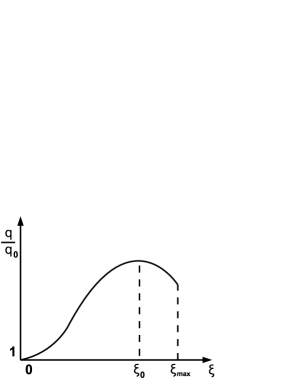
Figure 2: The $\hat{q}/\hat{q}_{0}$ ratio for the case of one nonzero angular parameter and the CE plotted as a function of the dimensionless parameter $0\leqslant\xi\leqslant\xi_{\rm max}$ in (2.25). The maximum and final values occurring at $\xi_{0}=1.09$ and $\xi_{\rm max}=1.33$ are ${\hat{q}\over\hat{q}_{0}}=1.37$ and $1.19$, respectively. The corresponding plot for the GCE in terms of the parameter $0\leqslant\hat{\xi}\leqslant{1\over 2}$ in (2.30) is similar in shape. The maximum and final values occurring at $\hat{\xi}_{0}=0.499$ and $\hat{\xi}_{\rm max}={1\over 2}$, are ${\hat{q}\over\hat{q}_{0}}=1.369$ and $1.368$, respectively. Note the closeness of the maximum and final values in the GCE case.

As mentioned in the introduction, an alternative, but not apparently equivalent, description of the problem of energy loss in the plasma is provided by the drag force felt by a particle passing through the medium. In this latter context, the authors of [21], utilizing the same metric (2.21), showed that the drag force is an increasing function of the R-charge for small values of a parameter similar to $\xi$. In this perturbative regime, this is in qualitative agreement with our results. On the other hand, we have shown that the ratio $\hat{q}/\hat{q}_{0}$ reaches a maximum at a finite value of $\xi$ (or $\hat{\xi}$) lower than its maximal value. In [20], a computation of the drag force was performed using a five-dimensional black hole solution [34] arising from the dimensionally reduced spinning D3-brane solutions that we have been using. Indeed, in that case the drag force exhibits a behavior (see fig. 2 of [20]) sensitive to the number of equal nonzero angular momenta, which is qualitatively in agreement with expectations based on our computation of the jet quenching parameter.

Note added. While this paper was being typewritten, we received [35] and [36] whose results partially overlap with those of section 3.3.

Acknowledgments

We would like to thank D. Zoakos for helpful discussions. K. S. acknowledges support provided through the European Community’s program “Constituents, Fundamental Forces and Symmetries of the Universe” with contract MRTN-CT-2004-005104, the INTAS contract 03-51-6346 “Strings, branes and higher-spin gauge fields”, the Greek Ministry of Education programs $\rm\Pi Y\Theta A\Gamma OPA\Sigma$ with contract 89194 and the program $\rm E\Pi AN$ with code-number B.545.

References

• [1]
• [2] E. Shuryak, Prog. Part. Nucl. Phys.  53 (2004) 273, hep-ph/0312227 and Nucl. Phys. A750 (2005) 64, hep-ph/0405066. M.J. Tannenbaum, Recent results in relativistic heavy ion collisions: from “a new state of matter” to “a perfect fluid”, nucl-ex/0603003.
• [3] D. Teaney, J. Lauret and E. Shuryak, A hydrodynamic description of heavy ion collisions at the SPS and RHIC, nucl-th/0110037. P.F. Kolb and U.W. Heinz, Hydrodynamic description of ultrarelativistic heavy-ion collisions, nucl-th/0305084.
• [4] J.M. Maldacena, Adv. Theor. Math. Phys.  2 (1998) 231, Int. J. Theor. Phys.  38 (1999) 1113, hep-th/9711200. S.S. Gubser, I.R. Klebanov and A.M. Polyakov, Phys. Lett. B428 (1998) 105, hep-th/9802109. E. Witten, Adv. Theor. Math. Phys. 2 (1998) 253, hep-th/9802150.
• [5] G. Policastro, D.T. Son and A.O. Starinets, Phys. Rev. Lett.  87 (2001) 081601, hep-th/0104066, JHEP 0209 (2002) 043, hep-th/0205052 and JHEP 0212 (2002) 054, hep-th/0210220. A. Buchel, J.T. Liu and A.O. Starinets, Nucl. Phys. B707 (2005) 56, hep-th/0406264. D.T. Son and A.O. Starinets, JHEP 0603 (2006) 052, hep-th/0601157.
• [6] P. Kovtun, D.T. Son and A.O. Starinets, JHEP 0310 (2003) 064, hep-th/0309213, and Phys. Rev. Lett.  94 (2005) 111601, hep-th/0405231. A. Buchel and J.T. Liu, Phys. Rev. Lett.  93 (2004) 090602, hep-th/0311175. A. Buchel, Phys. Lett. B609 (2005) 392, hep-th/0408095.
• [7] J. Mas, JHEP 0603 (2006) 016, hep-th/0601144. K. Maeda, M. Natsuume and T. Okamura, Phys. Rev.  D73 (2006) 066013, hep-th/0602010.
• [8] J.D. Bjorken, Energy Loss Of Energetic Partons In Quark - Gluon Plasma: Possible Extinction Of High P(T) Jets In Hadron - Hadron Collisions, FERMILAB-PUB-82-059-THY. M. Gyulassy and M. Plümer, Phys. Lett. B243 (1990) 432. M.H. Thoma and M. Gyulassy, Nucl. Phys. B351 (1991) 491. R. Baier, D. Schiff and B.G. Zakharov, Ann. Rev. Nucl. Part. Sci.  50 (2000) 37, hep-ph/0002198. B. Müller, Phys. Rev. C67 (2003) 061901, nucl-th/0208038. M. Gyulassy, I. Vitev, X.N. Wang and B.W. Zhang, Jet quenching and radiative energy loss in dense nuclear matter, nucl-th/0302077.
• [9] A. Kovner and U.A. Wiedemann, Phys. Rev. D64 (2001) 114002, hep-ph/0106240.
• [10] U.A. Wiedemann, Nucl. Phys. B588 (2000) 303, hep-ph/0005129. A. Kovner and U.A. Wiedemann, Gluon radiation and parton energy loss, hep-ph/0304151.
• [11] R. Baier, Y.L. Dokshitzer, A.H. Mueller, S. Peigné and D. Schiff, Nucl. Phys. B484 (1997) 265, hep-ph/9608322.
• [12] J.M. Maldacena, Phys. Rev. Lett. 80 (1998) 4859, hep-th/9803002. S.J. Rey and J.T. Yee, Eur. Phys. J. C22 (2001) 379, hep-th/9803001.
• [13] S.J. Rey, S. Theisen and J.T. Yee, Nucl. Phys. B527 (1998) 171, hep-th/9803135. A. Brandhuber, N. Itzhaki, J. Sonnenschein and S. Yankielowicz, Phys. Lett. B434 (1998) 36, hep-th/9803137.
• [14] A. Brandhuber and K. Sfetsos, Adv. Theor. Math. Phys. 3 (1999) 851, hep-th/9906201.
• [15] H. Liu, K. Rajagopal and U. A. Wiedemann, Phys. Rev. Lett.  97 (2006) 182301, hep-ph/0605178.
• [16] C.P. Herzog, A. Karch, P. Kovtun, C. Kozcaz and L.G. Yaffe, JHEP 0607 (2006) 013, hep-th/0605158.
• [17] S.S. Gubser, Drag force in AdS/CFT, hep-th/0605182.
• [18] J. Casalderrey-Solana and D. Teaney, Phys. Rev. D74 (2006) 085012, hep-ph/0605199.
• [19] J.J. Friess, S.S. Gubser and G. Michalogiorgakis, JHEP 0609 (2006) 072, hep-th/0605292.
• [20] C.P. Herzog, JHEP 0609 (2006) 032, hep-th/0605191.
• [21] E. Cáceres and A. Guijosa, JHEP 0611 (2006) 077, hep-th/0605235.
• [22] M. Chernicoff, J.A. Garcia and A. Guijosa, JHEP 0609 (2006) 068, hep-th/0607089.
• [23] H. Liu, K. Rajagopal and U.A. Wiedemann, Wilson loops in heavy ion collisions and their calculation in AdS/CFT, hep-ph/0612168.
• [24] P.C. Argyres, M. Edalati and J.F. Vázquez-Poritz, Spacelike strings and jet quenching from a Wilson loop, hep-th/0612157.
• [25] H. Liu, K. Rajagopal and U.A. Wiedemann, An AdS/CFT calculation of screening in a hot wind, hep-ph/0607062.
• [26] A. Buchel, Phys. Rev. D74 (2006) 046006, hep-th/0605178.
• [27] E. Witten, Adv. Theor. Math. Phys.  2 (1998) 505, hep-th/9803131.
• [28] P. Kraus, F. Larsen and S.P. Trivedi, JHEP 9903 (1999) 003, hep-th/9811120.
• [29] M. Cvetic and D. Youm, Nucl. Phys. B477 (1996) 449, hep-th/9605051
• [30] J.G. Russo and K. Sfetsos, Adv. Theor. Math. Phys.  3 (1999) 131, hep-th/9901056.
• [31] S.S. Gubser, Nucl. Phys. B551 (1999) 667, hep-th/9810225. R.G. Cai and K.S. Soh, Mod. Phys. Lett. A14 (1999) 1895, hep-th/9812121.
• [32] M. Cvetic and S.S. Gubser, JHEP 9907 (1999) 010, hep-th/9903132.
• [33] T. Harmark and N.A. Obers, JHEP 0001 (2000) 008, hep-th/9910036.
• [34] K. Behrndt, M. Cvetic and W.A. Sabra, Nucl. Phys. B553 (1999) 317, hep-th/9810227.
• [35] E. Cáceres and A. Guijosa, On Drag Forces and Jet Quenching in Strongly Coupled Plasmas, hep-th/0606134.
• [36] F.L. Lin and T. Matsuo, Phys. Lett. B641 (2006) 45, hep-th/0606136.