DESY 06-059 June 2006 Supersymmetric Standard Model
from the Heterotic String (II)

Abstract

We describe in detail a $\mathbbm{Z}_{6}$ orbifold compactification of the heterotic $\mathrm{E}_{8}\times\mathrm{E}_{8}$ string which leads to the (supersymmetric) standard model gauge group and matter content. The quarks and leptons appear as three ${\bf 16}$-plets of $\mathrm{SO}(10)$, two of which are localized at fixed points with local $\mathrm{SO}(10)$ symmetry. The model has supersymmetric vacua without exotics at low energies and is consistent with gauge coupling unification. Supersymmetry can be broken via gaugino condensation in the hidden sector. The model has large vacuum degeneracy. Certain vacua with approximate $B\!-\!L$ symmetry have attractive phenomenological features. The top quark Yukawa coupling arises from gauge interactions and is of the order of the gauge couplings. The other Yukawa couplings are suppressed by powers of standard model singlet fields, similarly to the Froggatt-Nielsen mechanism.

1 Introduction and Summary

The standard model is a remarkably successful theory of the structure of matter. It is a chiral gauge theory with the gauge group $G_{\mathrm{SM}}=\mathrm{SU}(3)_{c}\times\mathrm{SU}(2)_{\mathrm{L}}\times\mathrm{U}(1)_{Y}$ and three generations of quarks and leptons. All masses are generated by the Higgs mechanism which involves an $\mathrm{SU}(2)$ doublet of scalar fields. Its unequivocal prediction is the existence of the Higgs boson which still remains to be discovered. From a theoretical perspective, the minimal supersymmetric extension of the standard model, the MSSM, is particularly attractive. Apart from stabilizing the hierarchy between the electroweak and Planck scales and providing a natural explanation of the observed dark matter, it predicts unification of the gauge couplings at the unification scale $M_{\mathrm{GUT}}\simeq 2\cdot 10^{16}\,\mathrm{GeV}$.

Even more than the unification of gauge couplings, the symmetries and the particle content of the standard model point towards grand unified theories (GUTs) [1, 2]. Remarkably, one generation of matter, including the right-handed neutrino, forms a single spinor representation of $\mathrm{SO}(10)$ [3, 4]. It therefore appears natural to assume an underlying $\mathrm{SO}(10)$ structure of the theory. The route of unification, continuing via exceptional groups, terminates at $\mathrm{E}_{8}$, which is beautifully realized in the heterotic string [5, 6].

An obstacle on the path towards unification are the Higgs fields, which are $\mathrm{SU}(2)_{\mathrm{L}}$ doublets, while the smallest $\mathrm{SO}(10)$ representation containing the Higgs doublets, the $\boldsymbol{10}$–plet, predicts additional $\mathrm{SU}(3)_{c}$ triplets. The fact that Higgs fields form incomplete ‘split’ GUT representations is particularly puzzling in supersymmetric theories where both matter and Higgs fields are chiral multiplets. The triplets cannot have masses below $M_{\mathrm{GUT}}$ since otherwise proton decay would be too rapid. This then raises the question why $\mathrm{SU}(2)_{\mathrm{L}}$ doublets are so much lighter than $\mathrm{SU}(3)_{c}$ triplets. This is the notorious doublet-triplet splitting problem of ordinary 4D GUTs.

Higher-dimensional theories offer new possibilities for gauge symmetry breaking connected with compactification to four dimensions. A simple and elegant scheme, leading to chiral fermions in four dimensions, is the compactification on orbifolds, first considered for the heterotic string [7, 8, 9, 10, 11, 12, 13], and more recently applied to GUT field theories [14, 15, 16, 17, 18, 19]. Such orbifold GUTs appear as intermediate effective field theories in compactifications of the heterotic string when some of the compact dimensions are of order $1/M_{\mathrm{GUT}}$ and therefore large compared to the string length [20, 21, 22, 23].

In orbifold compactifications, gauge symmetry of the 4D effective theory is an intersection of larger symmetries at orbifold fixed points. Massless modes located at these fixed points all appear in the 4D theory and form representations of the larger local symmetry groups. Zero modes of bulk fields, on the contrary, are only representations of the smaller 4D gauge symmetry and form in general ‘split multiplets’. When the local symmetry at some orbifold fixed points is a GUT symmetry, one obtains the picture of ‘local grand unification’. The SM gauge group can be thought of as an intersection of different local GUT groups. Matter fields appear as complete GUT representations localized at the fixed points, whereas the Higgs doublets are associated with bulk fields, and therefore split multiplets. In this way the structure of the standard model is naturally reproduced [23, 24, 25].

Recently, we have obtained the gauge group and matter content of the supersymmetric standard model from the heterotic string by using the picture of local grand unification as the guiding principle [26]. Quarks and leptons appear as three $\boldsymbol{16}$–plets of $\mathrm{SO}(10)$, two of which are localized at orbifold fixed points with local $\mathrm{SO}(10)$ symmetry. For generic vacua, no exotic states appear at low energies and the model is consistent with gauge coupling unification. In this paper we describe our construction in detail.

It is well-known that the number of possible string vacua is huge. Early estimates of the total number of different vacua of the heterotic string gave numbers like $10^{1500}$ [27], which came as a complete surprise. More recent studies, based on flux compactifications, give similarly large numbers [28]. Searches for standard model–like vacua have been based on orbifold compactifications [29, 30], the free fermionic formulation [31, 32, 33], intersecting D–brane models [34] and Gepner orientifolds [35]. Despite the huge number of vacua, it turned out to be extremely difficult to construct a consistent ultraviolet completion of the (supersymmetric) standard model, and only recently several examples have been obtained [26, 36, 37]. This suggests that not all field theories can be embedded into string theory and that a consistent ultraviolet completion of the standard model may eventually lead to some testable low energy predictions.

In this paper, the model presented in [26] is described in detail. We hope that this will be useful for further phenomenological studies of the model and also for the search for other embeddings of the standard model into the heterotic string. In order to keep the paper self-contained, we recall the basics of strings on orbifolds in Secs. 2–4. In Sec. 2, the boundary conditions for untwisted and twisted strings, the mode expansion and the massless spectrum are discussed; furthermore, a simple derivation of the projection conditions for physical states is given. Our orbifold model is based on the 6D torus defined by the $\mathrm{G}_{2}\times\mathrm{SU}(3)\times\mathrm{SO}(4)$ root lattice, which has a $\mathbbm{Z}_{6-\mathrm{II}}=\mathbbm{Z}_{3}\times\mathbbm{Z}_{2}$ discrete symmetry. The geometry is described in Sec. 3 with emphasis on the localization of twisted states. In Sec. 4, the string selection rules for superpotential couplings of the $\mathbbm{Z}_{6-\mathrm{II}}$ orbifold are reviewed and somewhat extended.

The main results of this paper are contained in Secs. 5–8 and in the appendices A–D. After describing our search strategy for compactifications with local $\mathrm{SO}(10)$ symmetry, we study the unbroken gauge group $G$ and the massless spectrum of the model in Sec. 5. We also list the GUT representations at various fixed points and the 6D orbifold GUTs which one obtains for two compact dimensions of size $1/M_{\mathrm{GUT}}$. The Fayet-Iliopoulos (FI) $D$-term of an anomalous $\mathrm{U}(1)$ triggers further symmetry breaking [39]. In particular,

$$G~{}\longrightarrow~{}\mathrm{SU}(3)_{c}\times\mathrm{SU}(2)_{\mathrm{L}}\times\mathrm{U}(1)_{Y}\times G_{\mathrm{hidden}}\;,$$ (1.1)

with $G_{\mathrm{hidden}}=\mathrm{SU}(4)\times\mathrm{SU}(2)^{\prime}$ is possible, in which case the model has a truly hidden sector admitting spontaneous SUSY breaking. We further show that, for generic vacua, unwanted exotic states attain large masses and decouple. This is one of the central results of our paper.

The decoupling of exotic states can be achieved without breaking supersymmetry. In Sec. 6, we discuss $D$- and $F$-flat directions in the field space as well as general supersymmetric field configurations, neglecting supergravity corrections. The model naturally accommodates spontaneous supersymmetry breaking via hidden sector gaugino condensation, which is described in Sec. 7.

In generic $F$– and $D$–flat configurations, our model yields the MSSM spectrum, however the analysis of proton decay and flavour becomes intractable. In Sec. 8, we therefore identify a simple and phenomenologically attractive $D$–flat field configuration, without proving $F$–flatness, which preserves

$$G_{\mathrm{SM}}\times\mathrm{U}(1)_{B\!-\!L}\times[\mathrm{SU}(4)]\;.$$ (1.2)

Here we keep the hidden sector $\mathrm{SU}(4)$ unbroken which is needed for gaugino condensation. We show that unwanted exotics can be decoupled in this case as well. Further, we identify two Higgs doublets and discuss the pattern of Yukawa couplings. The top quark Yukawa coupling arises from gauge interactions and is of the order of the gauge couplings. Other Yukawa couplings are suppressed by powers of standard model singlet fields, similarly to the Froggatt–Nielsen mechanism [40].

Finally, in Sec. 9, we conclude with a brief outlook on open questions and further challenges for realistic compactifications of the heterotic string.

2 Strings on orbifolds

In the following subsections we collect the basic notions and formulae which are needed to describe propagation of the $\mathrm{E}_{8}\times\mathrm{E}_{8}$ heterotic string on orbifolds $\mathbbm{T}^{6}/\mathbbm{Z}_{N}$ [7, 8]. We follow the definitions of Katsuki et al. [41].

2.1 Lattices and twists

The torus is obtained as the quotient $\mathbbm{T}^{6}=\mathbbm{R}^{6}/2\pi\Lambda$, where $\Lambda$ is the lattice of a semi–simple Lie algebra of rank 6 with a $\mathbbm{Z}_{N}$ discrete symmetry. The 6 compact coordinates of the torus $x^{i}$, $i=4\ldots 9$, are conveniently combined into 3 complex coordinates $z^{i}={1\over\sqrt{2}}\left(x^{2i+2}+\mathrm{i}x^{2i+3}\right)$, $i=1\ldots 3$. Points in $\mathbbm{R}^{6}$ differing by a lattice vector,

$$z~{}\sim~{}z+2\pi\ell\;,$$ (2.1)

with $\ell=m_{a}e_{a}$, $m_{a}\in\mathbbm{Z}$ ($a=1\ldots 6$), are identified. Here $e_{a}$ denote the basis vectors in the three planes of the lattice.

The lattice has a $\mathbbm{Z}_{N}$ discrete symmetry which acts crystallographically, i.e., it maps the lattice onto itself,

$$z~{}\rightarrow~{}\theta z\;,\quad\theta^{i}_{j}~{}=~{}e^{2\pi\mathrm{i}v_{N}^{i}}\delta^{i}_{j}\;,\quad i,j=1\ldots 3\;,$$ (2.2)

with

$$\theta^{N}~{}=~{}1\;,\quad Nv_{N}^{i}=0\mod 1\;.$$ (2.3)

Here we assume the factorization $\mathbbm{T}^{6}=\mathbbm{T}^{2}\otimes\mathbbm{T}^{2}\otimes\mathbbm{T}^{2}$. $N=1$ supersymmetry in 4D requires that the $\mathbbm{Z}_{N}$ twist be contained in the $\mathrm{SU}(3)$ subgroup of $\mathrm{SO}(6)$, i.e.,

$$\sum_{i}v_{N}^{i}=0\mod 1\;.$$ (2.4)

Lattice translations and twists $\theta^{k}$ ($k=0,\dots,N-1$) form the space group $\mathbbm{S}$ whose elements are denoted by $(\theta^{k},\ell)$. The orbifold $\mathbbm{T}^{6}/\mathbbm{Z}_{N}$ can also be defined as the quotient $\mathbbm{R}^{6}/\mathbbm{S}$, where

$$z~{}\sim~{}(\theta^{k},\ell)\,z~{}\equiv~{}\theta^{k}\,z+2\pi\,\ell\;.$$ (2.5)

The multiplication rule in the space group is given by

$$(\theta^{k_{1}},\ell_{1})(\theta^{k_{2}},\ell_{2})~{}=~{}(\theta^{k_{1}}\theta^{k_{2}},\theta^{k_{1}}\ell_{2}+\ell_{1})\;.$$ (2.6)

An orbifold has fixed points $f$, which are invariant under the action of a space group element $(\theta^{k},\ell)$,

$$f~{}=~{}(\theta^{k},\ell)\,f~{}=~{}\theta^{k}\,f+2\pi\,\ell\;,\quad\ell~{}=~{}m_{a}\,e_{a}\;,\quad m_{a}\in\mathbbm{Z}\;.$$ (2.7)

Here $k$ and $\ell$ depend on the fixed point $f$. Since the position of the fixed point is defined only up to a lattice vector, $\ell$ is defined up to a translation in the sublattice

$$\Lambda_{k}~{}\equiv~{}(\mathbbm{1}-\theta^{k})\,\Lambda~{}=~{}\left\{\lambda\in\Lambda|\ \lambda=(\mathbbm{1}-\theta^{k})\,\mu,\;\mu\in\Lambda\right\}\;.$$ (2.8)

Each fixed point $(\theta^{k},\ell)$ is associated with a sublattice $\Lambda=\ell+\Lambda_{k}$, and there are as many sublattices as fixed points. The dimension of a sublattice $\Lambda_{k}$ can be smaller than $\dim\Lambda=6$ if $(\mathbbm{1}-\theta^{k})$ has eigenvectors with eigenvalue $0$. In this case the element $(\theta^{k},\ell)$ describes fixed planes.

2.2 Untwisted and twisted strings

In the light-cone gauge the heterotic string can be described by the following world-sheet fields [42]: 8 string coordinates and 8 right-moving Neveu-Schwarz-Ramond fermions ($\sigma_{\pm}=\tau\pm\sigma$),

$$X^{i}(\tau,\sigma)~{}=~{}X^{i}_{\mathrm{L}}(\sigma_{+})+X^{i}_{\mathrm{R}}(\sigma_{-})\;,\quad\psi^{i}(\sigma_{-})\;,\quad i=2\ldots 9\;,$$ (2.9)

and 32 left-moving fermions $\lambda^{I}$,

$$\lambda^{I}(\sigma_{+})\;,\quad I=1\ldots 32\;.$$ (2.10)

Here $i$ is the space–time index, while index $I$ is associated with $\mathrm{E}_{8}\times\mathrm{E}_{8}$ gauge degrees of freedom. It is convenient to combine the string coordinates in the compact dimensions into 3 complex variables $Z^{i}$ and, similarly, the right moving fermions into 3 complex NSR fermions $\widetilde{\psi}^{i}$,

$$Z^{i}~{}=~{}{1\over\sqrt{2}}\left(X^{2i+2}+\mathrm{i}X^{2i+3}\right)\;,\quad\widetilde{\psi}^{i}~{}=~{}{1\over\sqrt{2}}\left(\psi^{2i+2}+\mathrm{i}\psi^{2i+3}\right)\;,$$ (2.11)

where $i=1\ldots 3\;$. The $\mathbbm{Z}_{N}$ twist acts on these fields as

$$Z~{}\rightarrow~{}\theta\,Z\;,\quad\widetilde{\psi}~{}\rightarrow~{}\theta\,\widetilde{\psi}\;.$$ (2.12)

Closed strings on $\mathbbm{Z}_{N}$ orbifolds can be untwisted or twisted. In the former case the string is closed already on the torus and has the boundary conditions,

$$Z(\sigma+2\pi) = Z(\sigma)+2\pi m_{a}e_{a}\;,\quad m_{a}\in\mathbbm{Z}\;,$$ (2.13)

$$\widetilde{\psi}(\sigma+2\pi) = \pm\ \widetilde{\psi}(\sigma)\;,$$ (2.14)

whereas in the latter case the string is closed on the orbifold but not on the torus and has the boundary conditions ($k=1\ldots N-1$),

$$Z(\sigma+2\pi) = \theta^{k}\,Z(\sigma)+2\pi\,m_{a}\,e_{a}\;,$$ (2.15)

$$\widetilde{\psi}(\sigma+2\pi) = \pm\,\theta^{k}\,\widetilde{\psi}(\sigma)\;,$$ (2.16)

where $k$ and $m_{a}$ depend on the fixed point $f$. The lattice translation in Eq. (2.15) enters the space group element associated with the fixed point, Eq. (2.7). The plus and minus signs in Eqs. (2.14) and (2.16) correspond to the Ramond and the Neveu-Schwarz sectors, respectively. Twisted strings are localized at the orbifold fixed points, whereas untwisted strings can propagate freely on the orbifold (Fig. 1).

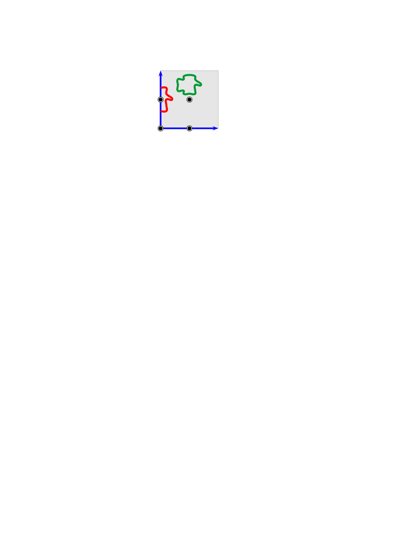
Figure 1: Twisted and untwisted strings. The dots denote orbifold fixed points.

Modular invariance usually requires that the $\mathbbm{Z}_{N}\subset\mathrm{SO}(6)$ twist of the space–time degrees of freedom be accompanied by a $\mathbbm{Z}_{N}\subset\mathrm{E}_{8}\times\mathrm{E}_{8}$ twist of the fermions $\lambda^{I}$, representing the internal symmetry group. On the complex fermions

$$\widetilde{\lambda}^{I}~{}=~{}{1\over\sqrt{2}}\left(\lambda^{2I-1}+\mathrm{i}\lambda^{2I}\right)\;,\quad I=1\ldots 16\;,$$ (2.17)

the $\mathbbm{Z}_{N}$ twist acts as

$$\widetilde{\lambda}~{}\rightarrow~{}\Theta\,\widetilde{\lambda}\;,\quad\Theta^{I}_{J}~{}=~{}e^{2\pi\mathrm{i}\,V^{I}_{N}}\,\delta^{I}_{J}\;,$$ (2.18)

where

$$\Theta^{N}=1\;,\quad N\sum_{I=1}^{8}V_{N}^{I}=N\sum_{I=9}^{16}V_{N}^{I}=0\mod 2\;,$$ (2.19)

with integer $NV_{N}^{I}$. The fermions $\widetilde{\lambda}^{I}$ can have untwisted ($k=0$) or twisted ($k=1\ldots N-1$) boundary conditions,

$$\widetilde{\lambda}(\sigma+2\pi)~{}=~{}\pm\Theta^{k}\,\widetilde{\lambda}(\sigma)\;.$$ (2.20)

This makes the parallel between $\theta$ and $\Theta$ transparent. Extending $v_{N}$ by a zero entry acting on the uncompactified dimensions, $v_{N}\rightarrow(v_{N}^{1},v_{N}^{2},v_{N}^{3};0)$, we note that vectors $Nv_{N}$ and $NV_{N}$ lie on the root lattices $\Lambda_{\mathrm{SO}(8)}$ and $\Lambda_{\mathrm{SO}(16)\times\mathrm{SO}(16)}$, respectively. In an orthonormal basis, $\Lambda_{\mathrm{SO}(2N)}$ is defined by vectors $(n_{1},\dots,n_{N})$ with integer $n_{i}$ and $\sum_{i=1}^{N}n_{i}=0\mod 2$. One can show that the gauge symmetry of this theory is $\mathrm{E}_{8}\times\mathrm{E}_{8}$ which contains $\mathrm{SO}(16)\times\mathrm{SO}(16)$ as a subgroup [6].

A convenient formulation of the heterotic string is obtained by representing fermionic degrees of freedom in terms of bosons. In this case one replaces the 8 right–moving and 32 left–moving fermions with 4 right–moving and 16 left–moving bosons,

$$\widetilde{\psi}^{i}(\sigma_{-}) = e^{-2\mathrm{i}\,H^{i}(\sigma_{-})}\;,\quad i=1\ldots 4\;,$$ (2.21)

$$\widetilde{\lambda}^{I}(\sigma_{+}) = e^{2\mathrm{i}\,X^{I}(\sigma_{+})}\;,\quad I=1\ldots 16\;.$$ (2.22)

The fields $X^{I}$ are compactified on a 16–dimensional torus represented by the $\mathrm{E}_{8}\times\mathrm{E}_{8}$ root lattice,

$$\Lambda_{\mathrm{E}_{8}}:\quad p=(n_{1},...,n_{8})\;\;{\rm or}\;\;\left(n_{1}+{1\over 2},...,n_{8}+{1\over 2}\right)\;,$$ (2.23)

where $n_{i}$ integer with $\sum_{i=1}^{8}n_{i}=0\mod 2$, and similarly for the second $\mathrm{E}_{8}$. This gives rise to gauge multiplets of the $\mathrm{E}_{8}\times\mathrm{E}_{8}$ group in 10 dimensions, coupled to supergravity.

Compactifying the extra 6 dimensions on an orbifold amounts to modding the string coordinates by the space group and its gauge counterpart. The latter is obtained by embedding the twists and lattice shifts into gauge degrees of freedom $X^{I}$ as

$$(\theta^{k},m_{a}e_{a})~{}\longrightarrow~{}(\mathbbm{1},k\,V_{N}^{I}+m_{a}\,W_{na}^{I})\;,$$ (2.24)

where $W_{na}^{I}$ denotes a Wilson line of order $n$. Here $NV_{N}$ and $nW_{n}$ ($n\leq N$) are required to lie on the $\mathrm{E}_{8}\times\mathrm{E}_{8}$ root lattice. Thus, a twist of the space–time degrees of freedom is accompanied by a shift $kV_{N}$ of the gauge coordinates, while a torus lattice translation is accompanied by a gauge coordinate shift $m_{a}W_{na}$. This corresponds to generalizing the boundary condition (2.20) for the left–moving fermions to

$$\widetilde{\lambda}^{I}(\sigma+2\pi)~{}=~{}\pm e^{2\pi\mathrm{i}\,(kV^{I}_{N}+m_{a}W^{I}_{na})}\,\widetilde{\lambda}^{I}(\sigma)\;.$$ (2.25)

The bosonic field boundary conditions then read ($k=0\ldots N-1$)

$$H^{i}(\sigma+2\pi) = H^{i}(\sigma)-\pi\,k\,v_{N}^{i}\mod\pi\,\Lambda_{\mathrm{SO}(8)}^{*}\;,$$ (2.26a)

$$X^{I}(\sigma+2\pi) = X^{I}(\sigma)+\pi\,\left(k\,V_{N}^{I}+m_{a}\,W_{na}^{I}\right)\mod\pi\,\Lambda_{\mathrm{E}_{8}\times\mathrm{E}_{8}}\;.$$ (2.26b)

Here $\Lambda_{\mathrm{SO}(8)}^{*}$ denotes the weight lattice of $\mathrm{SO}(8)$ given in the orthonormal basis by

$$\Lambda_{\mathrm{SO}(8)}^{*}:\quad q=(n_{1},n_{2},n_{3},n_{4})\;,$$ (2.27)

where $n_{i}$ integer with $\sum_{i}n_{i}$ odd or $n_{i}$ half-integer with $\sum_{i}n_{i}$ even.

To summarize, the heterotic string can be described by the left moving bosonic fields $Z^{i}_{\mathrm{L}}(\sigma_{+})$, $Z^{i*}_{\mathrm{L}}(\sigma_{+})$, $X^{I}(\sigma_{+})$ and the right moving bosonic fields $Z^{i}_{\mathrm{R}}(\sigma_{-})$, $Z^{i*}_{\mathrm{R}}(\sigma_{-})$, $H^{i}(\sigma_{-})$. They fall into untwisted or twisted categories depending on whether they represent strings closed on a torus or on an orbifold only.

2.3 Modular invariance and local twists

The gauge shift $V_{N}$ and the Wilson lines $W_{n}$ are subject to consistency conditions. First of all, $NV_{N}$ and $nW_{n}$ are vectors of the $\mathrm{E}_{8}\times\mathrm{E}_{8}$ root lattice,

$$N\,V_{N}~{}\in~{}\Lambda_{\mathrm{E}_{8}\times\mathrm{E}_{8}}\;,\quad n\,W_{n}~{}\in~{}\Lambda_{\mathrm{E}_{8}\times\mathrm{E}_{8}}\;.$$ (2.28)

Second, modular invariance of the theory requires that they satisfy additional constraints (see e.g., [21]):

$$N\;\left(V_{N}^{2}-v_{N}^{2}\right) = 0\mod 2\;,$$ (2.29a)

$$N\;V_{N}\cdot W_{n} = 0\mod 1\;,$$ (2.29b)

$$N\;W_{n}\cdot W_{m} = 0\mod 1\;,\quad(W_{n}\neq W_{m})$$ (2.29c)

$$N\;W_{n}^{2} = 0\mod 2\;.$$ (2.29d)

By adding $\mathrm{E}_{8}\times\mathrm{E}_{8}$ root lattice vectors to $V_{N}$ and $W_{n}$ satisfying these conditions, one can bring $V_{N}$,$W_{n}$ to the form which obeys a stronger constraint,

$$\frac{1}{2}\,\left(V_{N}^{2}-v_{N}^{2}\right) = 0\mod 1\;,$$ (2.30a)

$$V_{N}\cdot W_{n} = 0\mod 1\;,$$ (2.30b)

$$W_{n}\cdot W_{m} = 0\mod 1\;,\quad(W_{n}\neq W_{m})$$ (2.30c)

$$\frac{1}{2}\,W_{n}^{2} = 0\mod 1\;.$$ (2.30d)

This form has the advantage that the analysis of physical states of the theory simplifies significantly. These equations can also be written as

$$\frac{1}{2}\left[\left(rV_{N}+m_{a}\,W_{na}\right)^{2}-r^{2}v_{N}^{2}\right]~{}=~{}0\mod 1\;,\quad r=0,1\;,$$ (2.31)

where $0\leq m_{a}\leq n-1$ for a Wilson line $W_{n}$ of order $n$.

The twist can be thought of as a local quantity, that is, depending on the fixed point and the twisted sector. Indeed, Eqs. (2.25) and (2.26b) show that what matters at a particular fixed point $f$ is the combination

$$V_{f}^{I}~{}=~{}k\,V^{I}_{N}+m_{a}\,W^{I}_{na}\;,$$ (2.32)

which plays the role of the “local” gauge twist, as well as its right–moving counterpart $k\,v_{N}$. Each local twist $V_{f}$ can be expressed as the sum of the twist $k\,V_{N}$ for vanishing Wilson lines and a linear combination of Wilson lines determined by the location of the fixed point $f$. The local twists satisfy modular invariance conditions (2.31) and can be treated on the same footing as $V_{N}$. This observation will be important for the concept of local GUTs.

2.4 Mode expansion and massless spectrum

The boundary conditions discussed in Sec. 2.2 lead to the following mode expansion for the untwisted string ($i=1\ldots 3$),

$$Z^{i}(\tau,\sigma) = z^{i}+{1\over 2}p^{i}\tau+m_{a}e^{i}_{a}\sigma$$ (2.33a)

$${}+{\mathrm{i}\over 2}\sum_{n}{1\over n}\alpha^{i}_{n}e^{-\mathrm{i}n\sigma_{-}}+{\mathrm{i}\over 2}\sum_{n}{1\over n}\widetilde{\alpha}^{i}_{n}e^{-\mathrm{i}n\sigma_{+}}\;,$$

$$Z^{*i}(\tau,\sigma) = z^{*i}+{1\over 2}p^{*i}\tau+m_{a}\,e^{*i}_{a}\sigma$$ (2.33b)

$$+{\mathrm{i}\over 2}\sum_{n}{1\over n}\alpha^{*i}_{n}e^{-\mathrm{i}n\sigma_{-}}+{\mathrm{i}\over 2}\sum_{n}{1\over n}\widetilde{\alpha}^{*i}_{n}e^{-\mathrm{i}n\sigma_{+}}\;.$$

Twisted strings have the expansion (cf. Eq. (2.15))

$$Z^{i}(\tau,\sigma) = f^{i}+{\mathrm{i}\over 2}\sum_{n\in\mathbbm{Z}+kv_{N}^{i}}{1\over n}\alpha^{i}_{fn}e^{-\mathrm{i}n\sigma_{-}}+{\mathrm{i}\over 2}\sum_{n\in\mathbbm{Z}-kv_{N}^{i}}{1\over n}\widetilde{\alpha}^{i}_{fn}e^{-\mathrm{i}n\sigma_{+}}\;,$$ (2.34)

$$Z^{*i}(\tau,\sigma) = f^{*i}+{\mathrm{i}\over 2}\sum_{n\in\mathbbm{Z}-kv_{N}^{i}}{1\over n}\alpha^{*i}_{fn}e^{-\mathrm{i}n\sigma_{-}}+{\mathrm{i}\over 2}\sum_{n\in\mathbbm{Z}+kv_{N}^{i}}{1\over n}\widetilde{\alpha}^{*i}_{fn}e^{-\mathrm{i}n\sigma_{+}}\;.$$ (2.35)

In this case, there is no center–of–mass string motion, i.e., $p^{i}=m_{a}=0$. If there is a fixed plane, the boundary conditions for strings in the fixed plane are untwisted and the expansion is given by Eqs. (2.33).

The bosonized NSR fermions have the expansion ($i=1\ldots 4$)

$$H^{i}(\tau,\sigma)~{}=~{}h^{i}+{1\over 2}\left(q^{i}+kv_{N}^{i}\right)\sigma_{-}+{\mathrm{i}\over 2}\sum_{n\neq 0}{1\over n}\widetilde{\beta}^{i}_{n}e^{-\mathrm{i}n\sigma_{-}}\;,$$ (2.36)

while the gauge coordinates are given by ($I=1\ldots 16$)

$$X^{I}(\tau,\sigma)~{}=~{}x^{I}+{1\over 2}\left(p^{I}+\left(kV_{N}^{I}+m_{a}W^{I}_{na}\right)\right)\sigma_{+}+{\mathrm{i}\over 2}\sum_{n\neq 0}{1\over n}\widetilde{\alpha}^{I}_{fn}e^{-\mathrm{i}n\sigma_{+}}\;.$$ (2.37)

The momentum vectors $q^{i}$ and $p^{I}$ specify the Lorentz and gauge quantum numbers of the string states. Note that the creation and annihilation operators of the twisted string (2.34), (2.35) and the left-moving string (2.37) depend on the fixed point $f$.

States of the heterotic string are given by a direct product of the right–moving and left–moving parts. A basis in the Hilbert space of the quantised string is obtained by acting with the creation operators $\alpha^{i}_{fn}$, $\widetilde{\alpha}^{i}_{fn}$, $\widetilde{\beta}^{i}_{fn}$, $\widetilde{\alpha}^{I}_{fn}$ ($n<0$) on the ground states of the untwisted sector $U$ ($k=0$) and the twisted sectors $T_{k}$ ($k=1\ldots N-1$). Massless states in the untwisted sector as well as twisted states living on fixed planes have $p^{i}=m_{a}=0$. The ground states of the different sectors depend on the momentum vectors $q^{i}$, $p^{I}$ and, for the twisted sectors, also on the fixed point $f$ (cf. (2.32)),

$$|q,p\rangle~{}\equiv~{}|q\rangle\otimes|p\rangle\;,\quad|f;q,p\rangle~{}\equiv~{}|q+kv_{N}\rangle\otimes|p+V_{f}\rangle\;.$$ (2.38)

It turns out that for the model discussed below only oscillator modes of the left-moving strings $Z^{i}_{\mathrm{L}}(\sigma_{+})$, $Z^{*i}_{\mathrm{L}}(\sigma_{+})$ and $X^{I}(\sigma_{+})$ are relevant. The corresponding twisted sector states are ($n_{i},m_{i}<0$)

$$\widetilde{\alpha}^{i_{1}}_{fn_{1}}\widetilde{\alpha}^{i_{2}}_{fn_{2}}\ldots\widetilde{\alpha}^{*{j_{1}}}_{fm_{1}}\widetilde{\alpha}^{*{j_{2}}}_{fm_{2}}\ldots\widetilde{\alpha}^{*{I_{1}}}_{fl_{1}}\widetilde{\alpha}^{*{I_{2}}}_{fl_{2}}\ldots|f;q,p\rangle\;.$$ (2.39)

Massless states of the untwisted sector satisfy the following mass equations:

$$\frac{1}{8}m_{\mathrm{R}}^{2} = \frac{1}{2}q^{2}-\frac{1}{2}+N+N^{*}=0\;,$$ (2.40a)

$$\frac{1}{8}m_{\mathrm{L}}^{2} = \frac{1}{2}p^{2}-1+\widetilde{N}+\widetilde{N}^{*}=0\;,$$ (2.40b)

where $N,N^{*},\widetilde{N},\widetilde{N}^{*}$ are the integer oscillator numbers. Twisted massless states obey

$$\frac{1}{8}m_{\mathrm{R}}^{2} = \frac{1}{2}(q+k\,v_{N})^{2}-\frac{1}{2}+\delta c^{(k)}+\omega_{i}^{(k)}\,N_{fi}+\bar{\omega}_{i}^{(k)}\,N_{fi}^{*}=0\;,$$ (2.41a)

$$\frac{1}{8}m_{\mathrm{L}}^{2} = \frac{1}{2}(p+V_{f})^{2}-1+\delta c^{(k)}+\omega_{i}^{(k)}\,\widetilde{N}_{fi}+\bar{\omega}_{i}^{(k)}\,\widetilde{N}_{fi}^{*}=0\;,$$ (2.41b)

where

$$\delta c^{(k)}~{}=~{}\frac{1}{2}\sum_{i}\omega^{(k)}_{i}\,(1-\omega^{(k)}_{i})\;,$$ (2.42)

with $\omega^{(k)}_{i}\,=\,(k\,v_{N})_{i}\mod 1$, so that $0<\omega^{(k)}_{i}\leq 1$, and $\bar{\omega}^{(k)}_{i}\,=\,(-k\,v_{N})_{i}\mod 1$ so that $0<\bar{\omega}^{(k)}_{i}\leq 1$. This implies that $\omega^{(k)}_{i}=\bar{\omega}^{(k)}_{i}=1$ for $(k\,v_{N})_{i}$ integer. In Eq. (2.41), $N_{fi}$, $N_{fi}^{*}$, $\widetilde{N}_{fi}$ and $\widetilde{N}_{fi}^{*}$ $\in\mathbb{N}$ represent the oscillator numbers of the right- and left-movers in $z_{i}$ and $\bar{z}_{i}$ directions, respectively. Note that $N_{fi}$ and $N_{fi}^{*}$, as well as $\widetilde{N}_{fi}$ and $\widetilde{N}_{fi}^{*}$, denote independent quantities. They are the eigenvalues of the corresponding number operators $\hat{N}_{fi}$,

$$\hat{N}_{fi}~{}=~{}{1\over\omega^{(k)}_{i}}~{}\sum_{n>0}\alpha^{i}_{f-n}\alpha^{i}_{fn}\;,$$ (2.43)

and analogously for $N_{fi}^{*}$, $\widetilde{N}_{fi}$, $\widetilde{N}_{fi}^{*}$. The sum $\sum_{i}(\omega^{(k)}_{ki}\,\widetilde{N}_{fi}+\bar{\omega}^{(k)}_{ki}\,\widetilde{N}_{fi}^{*})$ is often referred to as $\widetilde{N}$ in the literature.

2.5 Projection conditions for physical states

As discussed in Sec. 2.2, an orbifold is obtained by identifying points in flat space which transform into each other under the action of the space group,

$$x~{}\sim~{}gx\;,\quad x\in\mathbbm{R}^{6}\;,\quad g\in\mathbbm{S}\;.$$ (2.44)

Quantized strings whose boundary conditions are related by a symmetry transformation must lead to the same Hilbert space of physical states. In particular, strings with the boundary conditions

$$\phi(\sigma+2\pi)~{}\sim~{}g\phi(\sigma)\quad{\rm and}\quad\phi(\sigma+2\pi)~{}\sim~{}hgh^{-1}\phi(\sigma)$$ (2.45)

produce the same Hilbert space for any $h\in\mathbbm{S}$ [8]. Here $\phi$ stands for $Z^{i}$, $Z^{*i}$, $H^{i}$ and $X^{I}$. For each conjugacy class consisting of elements $h\,g\,h^{-1}$ one therefore has a separate Hilbert space.

Space group elements $\bar{h}$ which commute with $g$, i.e. $\bar{h}\,g\,\bar{h}^{-1}=g$, leave the string boundary conditions invariant. Hence, their representation in the Hilbert space must act as the identity on physical states,

$$\bar{h}\,|\mathrm{phys}\rangle~{}=~{}|\mathrm{phys}\rangle\;.$$ (2.46)

This is the invariance or ‘projection’ condition for physical states.

A space group element $\bar{h}=(\theta^{\bar{k}},\bar{\ell})$ acts as a translation on the center–of–mass coordinates of the bosonic fields $H^{i}$ and $X^{I}$ (cf. (2.26)),

$$h^{i}~{}\rightarrow~{}h^{i}-\pi\,\bar{k}\,v_{N}^{i}\;,\quad x^{I}~{}\rightarrow~{}x^{I}+\pi\,\left(\bar{k}\,V_{N}^{I}+\bar{m}_{a}\,W^{I}_{na}\right)\;.$$ (2.47)

Hence, the momentum eigenstates in twisted sectors transform as

$$|f;q,p\rangle \rightarrow e^{2\pi\mathrm{i}\,(-\bar{k}\,v_{N}\cdot(q+kv_{N})+(\bar{k}\,V_{N}+\bar{m}_{a}\,W_{na})\cdot(p+V_{f}))}\,|f;q,p\rangle\;,$$ (2.48)

and similarly for untwisted states. From Eqs. (2.34) and (2.35) one reads off the transformation properties of the creation operators,

$$\widetilde{\alpha}^{i}_{fn}~{}\rightarrow~{}e^{2\pi\mathrm{i}\,\bar{k}\,v_{N}^{i}}\,\widetilde{\alpha}^{i}_{fn}\;,\quad\widetilde{\alpha}^{*i}_{fn}~{}\rightarrow~{}e^{-2\pi\mathrm{i}\,\bar{k}\,v_{N}^{i}}\,\widetilde{\alpha}^{*i}_{fn}\;.$$ (2.49)

A state with non–vanishing oscillator numbers then transforms as

$$\widetilde{\alpha}^{i}_{fn}\ldots\widetilde{\alpha}^{*i}_{fm}\ldots|f;q,p\rangle\rightarrow$$

$${}e^{2\pi\mathrm{i}\,\left(\bar{k}\,v_{N}\cdot\left(\widetilde{N}-\widetilde{N}^{*}\right)-\bar{k}\,v_{N}\cdot(q+kv_{N})+(\bar{k}\,V_{N}+\bar{m}_{a}\,W_{na})\cdot(p+V_{f})\right)}\,\widetilde{\alpha}^{i}_{fn}\ldots\widetilde{\alpha}^{*i}_{fm}\ldots|f;q,p\rangle\;.$$

Physical states have to satisfy Eq. (2.46), which yields the projection conditions

$$\bar{k}v_{N}\cdot\left(\widetilde{N}_{f}-\widetilde{N}_{f}^{*}\right)-\bar{k}v_{N}\cdot(q+kv_{N})$$ (2.51)

$$\hskip 85.35826pt{}+(\bar{k}V_{N}+\bar{m}_{a}\,W_{na})\cdot(p+V_{f})~{}=~{}0\mod 1\;,$$

for values of $\bar{k}$ and $\bar{m}^{a}$ which depend on the conjugacy class. As we will discuss in Sec. 2.5.2, in non–prime orbifolds Eq. (2.51) gets modified for higher twisted sector states. Below we analyze in detail the projection conditions for the untwisted and twisted sectors.

2.5.1 Untwisted sector

The untwisted sector ($k=0$) is associated with the space group element $g=(\mathbbm{1},0)$, and Eq. (2.51) has to be satisfied for the full space group, i.e., for all values $\bar{k}$ and $\bar{m}_{a}$. This yields the projection conditions

$$v_{N}\cdot q-V_{N}\cdot p~{}=~{}0~{}{\rm mod}~{}1\;,\quad W_{n}\cdot p~{}=~{}0~{}{\rm mod}~{}1\;,$$ (2.52)

where $p$ is the $\mathrm{E}_{8}\times\mathrm{E}_{8}$ root lattice momentum ($p^{2}=2$) and $q$ is the $\mathrm{SO}(8)$ weight lattice momentum ($q^{2}=1$). The $\mathrm{E}_{8}$ momenta lie on the same lattice as the $\mathrm{E}_{8}$ coordinates because of self-duality.

The untwisted sector contains gauge and matter supermultiplets of the 4D effective theory. For the former $v_{N}\cdot q=0$ mod 1 yielding gauge bosons with $q=(0^{3};\pm 1)$ and gauginos with $q=\pm\left(\tfrac{1}{2},\tfrac{1}{2},\tfrac{1}{2};\tfrac{1}{2}\right)$. For the matter multiplets, $v_{N}\cdot q=n/N$ mod 1 with $n=1,..,N-1$ leading to the bosonic $\mathrm{SO}(8)$ momenta $({\underline{\pm 1,0,0}};0)$ where the underline denotes permutations, and their fermionic partners.

Since gauge multiplets satisfy $v_{N}\cdot q=0$ mod 1, the conditions

$$V_{N}\cdot p~{}=~{}0~{}{\rm mod}~{}1\;,\quad W_{n}\cdot p~{}=~{}0~{}{\rm mod}~{}1\;,$$ (2.53)

determine the roots $p$ of the unbroken 4D gauge group. It is instructive to rewrite this set of equations as

$$V_{f}\cdot p~{}=~{}0~{}{\rm mod}~{}1\;,\quad\text{for all fixed points}\>f\;,$$ (2.54)

where $V_{f}$ is the local shift (2.32) associated with the fixed point. At each fixed point the gauge group is broken locally to a subgroup of $\mathrm{E}_{8}\times\mathrm{E}_{8}$. The states surviving all local projection conditions, i.e., those corresponding to the intersection of all local gauge groups, yield the gauge fields of the low-energy gauge group.

Matter multiplets ($v_{N}\cdot q\not=0$ mod 1) originate from the 10D gauge fields polarized in the compact directions and their fermionic partners. They form chiral superfields transforming as the coset of $\mathrm{E}_{8}\times\mathrm{E}_{8}$ and the unbroken 4D gauge group. All untwisted states are bulk fields in the compactified dimensions.

2.5.2 Twisted sectors

For the twisted sectors $T_{k}$ ($k=1\ldots N-1$), the projection conditions depend on $k$. Consider $k=1$ and a fixed point $f$ with the space group element $g=(\theta,\ell)$. The space group elements commuting with $g$ are $\bar{h}=(\theta^{\bar{k}},\bar{\ell})=(\theta,\ell)^{n}$, $n\in\mathbbm{N}$. The resulting projection condition is

$$v_{N}\cdot\left(\widetilde{N}_{f}-\widetilde{N}_{f}^{*}\right)-v_{N}\cdot(q+v_{N})+V_{f}\cdot(p+V_{f})~{}=~{}0\mod 1\;,$$ (2.55)

where $V_{f}=V_{N}+m_{a}W_{na}$. Using ‘strong’ modular invariance (2.30), one can show that all massless states (cf. (2.41)) satisfy this condition. Therefore all massless modes in the first twisted sector correspond to physical states. In the case of prime orbifolds, Eq. (2.55) also holds for higher twisted sectors with $V_{f}=k\,V_{N}+m_{a}\,W_{na}$.

For non–prime orbifolds the situation is more complicated. Some of the higher twisted sectors $T_{k}$, $k>1$, are related to lower order twists $\mathbb{Z}_{N/k}$ which leave one of the $\mathbb{T}^{2}$ tori invariant. This results in additional projection conditions. Furthermore, fixed points of the lower order twists are not necessarily fixed points of the original twist $\mathbb{Z}_{N}$. The $\mathbb{Z}_{N}$ twist transforms these fixed points into each other such that they are mapped into the same singular point in the fundamental domain of the orbifold. Physical states correspond to linear combinations of the states appearing at the fixed points of the $\mathbb{Z}_{N/k}$ twist.

The conjugacy classes of higher twisted sectors $T_{k}$ are given by $h\,g\,h^{-1}$ where both $g$ and $h$ have the form $(\theta^{k},\ell)$. The number of the conjugacy classes is the number of the fixed points of the lower order twist $\mathbb{Z}_{N/k}$. In general, twists of other orders $\mathbb{Z}_{N/k^{\prime}}$ transform these classes into each other. In particular, the $\mathbb{Z}_{N}$ twist acts on the $\mathbb{Z}_{N/k}$ conjugacy classes $g_{i}$ as

$$\bar{h}\,g_{1}\,\bar{h}^{-1}~{}=~{}g_{2}\;,\quad\bar{h}\,g_{2}\,\bar{h}^{-1}~{}=~{}g_{3}\;,\quad\dots\quad\bar{h}\,g_{n}\,\bar{h}^{-1}~{}=~{}g_{1}\;,$$ (2.56)

with $\bar{h}$ of the form $(\theta,\ell)$ and $n\geq 1$. In this case, the higher twisted states transform as

$$\bar{h}\,|1\rangle~{}=~{}|2\rangle\;,\quad\bar{h}\,|2\rangle~{}=~{}|3\rangle\;,\quad\dots\quad\bar{h}\,|n\rangle~{}=~{}|1\rangle\;.$$ (2.57)

From linear combinations of these localized states one obtains a basis of physical states which are $\mathbb{Z}_{N}$ twist and $\bar{h}$–eigenstates [8, 43, 44],

$$|\mathrm{phys},q_{\gamma}\rangle~{}=~{}\frac{1}{\sqrt{n}}\sum\limits_{s=1}^{n}e^{-2\pi\mathrm{i}\,s\,q_{\gamma}}|s\rangle\;,$$ (2.58)

where $q_{\gamma}=0,1/n,2/n,\dots,1$. As a consequence,

$$\bar{h}\,|\mathrm{phys},q_{\gamma}\rangle = e^{2\pi\mathrm{i}\,q_{\gamma}}\,e^{2\pi\mathrm{i}\left(\bar{k}v_{N}\cdot\left(\widetilde{N}_{f}-\widetilde{N}_{f}^{*}\right)-\bar{k}v_{N}\cdot(q+kv_{N})+(\bar{k}V_{N}+\bar{m}_{a}W_{a})\cdot(p+V_{f})\right)}\,$$ (2.59)

$$\times |\mathrm{phys},q_{\gamma}\rangle\;,$$

where we have used Eq. (LABEL:transf) and $\bar{h}=(\theta^{\bar{k}},\bar{m}_{a}\,e_{a})$ is assumed to mix the conjugacy classes of $T_{k}$ as above. This leads to the modified projection conditions for the superpositions (2.58):

$$\bar{k}v_{N}\cdot\left(\widetilde{N}_{f}-\widetilde{N}_{f}^{*}\right)-\bar{k}v_{N}\cdot(q+kv_{N})$$ (2.60)

$$\hskip 56.9055pt{}+(\bar{k}V_{N}+\bar{m}_{a}\,W_{na})\cdot(p+V_{f})+q_{\gamma}~{}=~{}0\mod 1\;.$$

In this paper we are especially interested in a $\mathbbm{Z}_{6-\mathrm{II}}$ orbifold which has $\mathbbm{Z}_{3}$ and $\mathbbm{Z}_{2}$ subtwists with invariant tori. The corresponding twist vector is $v_{6}=(-1/6,-1/3,1/2)$. As we shall discuss in detail in Sec. 3, two different fixed points in the $T_{2,4}$ twisted sectors are related by Eq. (2.56) with $\bar{h}=(\theta^{3},0)$. The eigenstates of $(\theta^{3},0)$ are

$$|\mathrm{phys},\pm\rangle~{}=~{}{1\over\sqrt{2}}\left(|1\rangle\pm|2\rangle\right)\;,$$ (2.61)

where the states $|1\rangle,|2\rangle$ correspond to the two fixed points of $\theta^{2}$ away from the origin. The projection condition (2.60) becomes

$$3v_{6}\cdot\left(\widetilde{N}_{f}-\widetilde{N}_{f}^{*}\right)-3v_{6}\cdot(q+k\,v_{6})+3V_{6}\cdot(p+V_{f})+q_{\gamma}~{}=~{}0\mod 1\;,$$ (2.62)

with $q_{\gamma}=1/2,1$ for $k=2,4$. Here $V_{f}=k\,V_{6}+m_{3}W_{3}$ is the local $\mathbbm{Z}_{3}$ gauge shift. Physical states of $T_{2,4}$ must also satisfy additional projection conditions which stem from invariance of the third $\mathbb{T}^{2}$ torus (‘the $\mathrm{SO}(4)$ torus’) under $\theta^{2}$. Clearly, translations $\ell_{3}$ in this torus commute with $\theta^{2}$. Thus invariance under space group transformations $(\mathbbm{1},\ell_{3})$ requires

$$W_{2}\cdot(p+V_{f}) = 0\mod 1\;,$$ (2.63a)

$$W^{\prime}_{2}\cdot(p+V_{f}) = 0\mod 1\;,$$ (2.63b)

where $W_{2}$ and $W_{2}^{\prime}$ are two discrete Wilson lines in the $\mathrm{SO}(4)$ torus.

The $\mathbbm{Z}_{6-\mathrm{II}}$ orbifold also has a $\mathbbm{Z}_{2}$ subtwist. The fixed points of the $T_{3}$ twisted sector are mapped into each other by the space group element $\bar{h}=(\theta^{2},0)$. Invariance under $\theta^{2}$ leads to the projection condition

$$2v_{6}\cdot\left(\widetilde{N}_{f}-\widetilde{N}_{f}^{*}\right)-2v_{6}\cdot(q+3v_{6})+2V_{6}\cdot(p+V_{f})+q_{\gamma}~{}=~{}0\mod 1\;,$$ (2.64)

with $q_{\gamma}=1/3,2/3,1$ and the local $\mathbbm{Z}_{2}$ gauge shift $V_{f}=3V_{6}+n_{2}W_{2}+n_{2}^{\prime}W_{2}^{\prime}$. The $\mathbbm{Z}_{2}$ twist leaves the second torus (‘the $\mathrm{SU}(3)$ torus’) invariant. Invariance of the $T_{3}$ states under translations in this torus requires

$$W_{3}\cdot(p+V_{f})~{}=~{}0\mod 1\;.$$ (2.65)

Here $W_{3}$ is a discrete Wilson line in the $\mathrm{SU}(3)$ torus.

$T_{5}$ twisted sector contains anti–particles of the $T_{1}$ sector, and will not be treated separately in the following.

The above projection conditions are relevant to our model. A sample calculation of the physical spectrum is given in App. A.

2.6 Local GUTs

Consider a fixed point $f$ which is associated with the local gauge shift $V_{f}^{I}=k\,V^{I}_{N}+m_{a}\,W^{I}_{na}$. A local GUT can be defined by the $\mathrm{E}_{8}\times\mathrm{E}_{8}$ roots $p$ ($p^{2}=2$) satisfying

$$p\cdot V_{f}~{}=~{}0\mod 1\;.$$ (2.66)

These roots represent a local gauge symmetry supported at the fixed point. Twisted matter appears in a representation of the local GUT. Each representation is characterized by the square of the shifted momentum, $(\widetilde{p}+V_{f})^{2}$, which is the same for members of the same multiplet.

The concept of local GUTs is important for construction of realistic models. In particular, all massless states of the $T_{1}$ sector survive the $\mathbbm{Z}_{N}$ projection and represent physical states. They form complete multiplets of the corresponding local GUT, although this GUT does not appear in 4D. As discussed in Sec. 1, this may naturally explain why the SM gauge (and Higgs) bosons do not form complete GUT multiplets, while the matter fields do.

Let us illustrate how a local SO(10) structure arises. Consider a $\mathbbm{Z}_{6-\mathrm{II}}$ heterotic orbifold based on the Lie lattice $\mathrm{G}_{2}\times\mathrm{SU}(3)\times\mathrm{SO}(4)$ with $v_{6}=(-1/6,-1/3,1/2;0)$, the gauge shift

$$V_{6}~{}=~{}\left(\frac{1}{2},\frac{1}{2},\frac{1}{3},0,0,0,0,0\right)\,\left(\frac{1}{3},0,0,0,0,0,0,0\right)\;,$$ (2.67)

and arbitrary Wilson lines.

The local gauge shift at the origin in the $T_{1}$ sector is $V_{f}=V_{6}$. The local GUT roots are found from

$$p\cdot V_{6}~{}=~{}0\mod 1\;.$$ (2.68)

This corresponds to $\mathrm{SO}(10)\times\mathrm{SU}(2)^{2}$ symmetry in the observable sector. The $\mathrm{SO}(10)$ roots are given by

$$p~{}=~{}(0,0,0,\underline{\pm 1,\pm 1,0,0,0})\;,$$ (2.69)

where the underline denotes all possible permutations of the corresponding entries.

Relevant twisted matter fields of the $T_{1}$ sector satisfy the masslessness condition

$$(p+V_{6})^{2}_{\mathrm{obs}}~{}=~{}{23\over 18}$$ (2.70)

for the $p+V_{6}$ components in the first $\mathrm{E}_{8}$. The solution is

$$(p+V_{6})_{\mathrm{obs}}~{}=~{}\left(0,0,-\tfrac{1}{6},\text{odd}\>(\pm\tfrac{1}{2})^{5}\right)\;,$$ (2.71)

where “odd $(\pm 1/2)^{5}$” denotes all combinations containing an odd number of minus signs. This is a $\boldsymbol{16}$–plet of $\mathrm{SO}(10)$. The $\mathbbm{Z}_{6}$ invariant states have the right–mover shifted momentum $q+v_{6}=(-1/6,-1/3,-1/2;0)$ for space–time bosons and analogously for space–time fermions. All of these states appear in the physical spectrum of the model.

The Wilson lines can be chosen such that the gauge group in 4D is that of the standard model (times extra factors). This does not affect the above considerations and the local $\mathrm{SO}(10)$ GUT structure remains intact.

3 Geometry of the $\boldsymbol{\mathbbm{Z}_{6-\mathrm{II}}}$ orbifold

In this section we describe geometrical features of the $\mathbbm{Z}_{6-\mathrm{II}}=\mathbbm{Z}_{3}\times\mathbbm{Z}_{2}$ orbifold based on the $\mathrm{G}_{2}\times\mathrm{SU}(3)\times\mathrm{SO}(4)$ Lie algebra lattice, which is required for construction of our model.

3.1 Fixed points and fundamental region

The $\mathbbm{Z}_{6-\mathrm{II}}$ orbifold with the $\mathrm{G}_{2}\times\mathrm{SU}(3)\times\mathrm{SO}(4)$ lattice is based on the twist vector

$$v_{6}~{}=~{}\frac{1}{6}(-1,-2,3;0)\;.$$ (3.1)

This orbifold allows for one discrete Wilson line of degree 3 in the $\mathrm{SU}(3)$ plane and two Wilson lines of degree 2 in the $\mathrm{SO}(4)$ plane. The $\mathbbm{Z}_{6}$ action on the torus coordinates $z^{i}$,

$$z^{i}\rightarrow e^{2\pi\mathrm{i}{v_{6}}^{i}}z^{i}\;,$$ (3.2)

is illustrated in Fig. 2. This orbifold has $\mathbbm{Z}_{6}$, $\mathbbm{Z}_{3}$ and $\mathbbm{Z}_{2}$ fixed points defined by

$$f^{i}-e^{2\pi\mathrm{i}\frac{6}{\kappa}{v_{6}}^{i}}f^{i}\in\Lambda_{\mathrm{G}_{2}\times\mathrm{SU}(3)\times\mathrm{SO}(4)}\;,\quad\kappa=6,3,2\;,$$ (3.3)

where $\Lambda_{\mathrm{G}_{2}\times\mathrm{SU}(3)\times\mathrm{SO}(4)}$ is the torus lattice. The 12 $\mathbbm{Z}_{6}$ fixed points are shown in Fig. 2, the 9 $\mathbbm{Z}_{3}$ fixed points – in Fig. 3 and the 16 $\mathbbm{Z}_{2}$ fixed points – in Fig. 4. It is a characteristic feature of non-prime orbifolds that the $\mathbbm{Z}_{3}$ and $\mathbbm{Z}_{2}$ fixed points are generally different from the $\mathbbm{Z}_{6}$ fixed points. The $\mathbbm{Z}_{3}$ subtwist leaves the $\mathrm{SO}(4)$ plane invariant, whereas under the $\mathbbm{Z}_{2}$ subtwist the $\mathrm{SU}(3)$ plane is fixed.

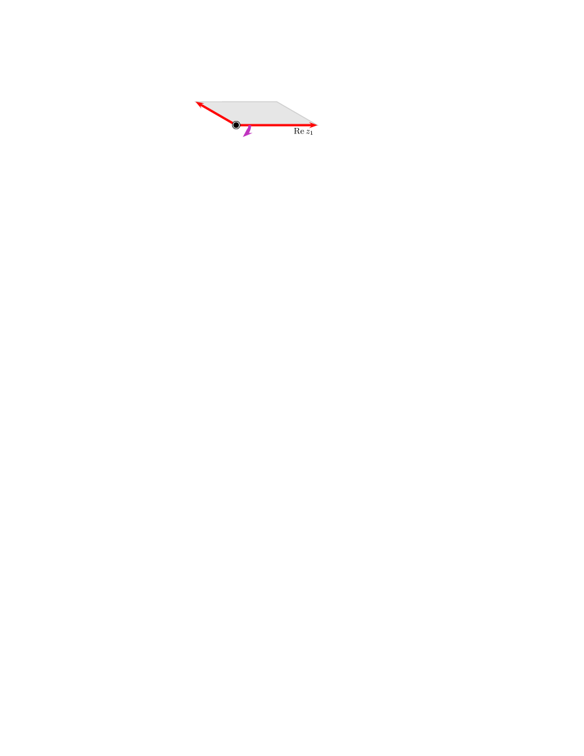
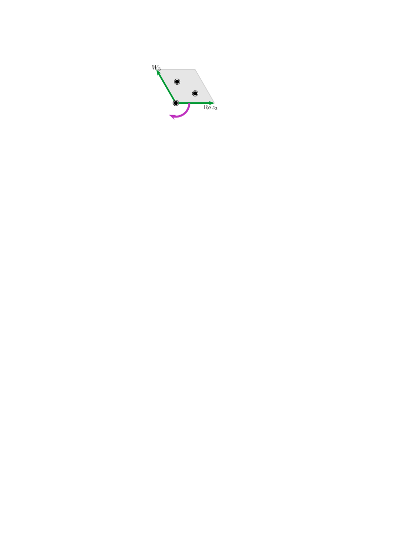
$\times$ $\times$

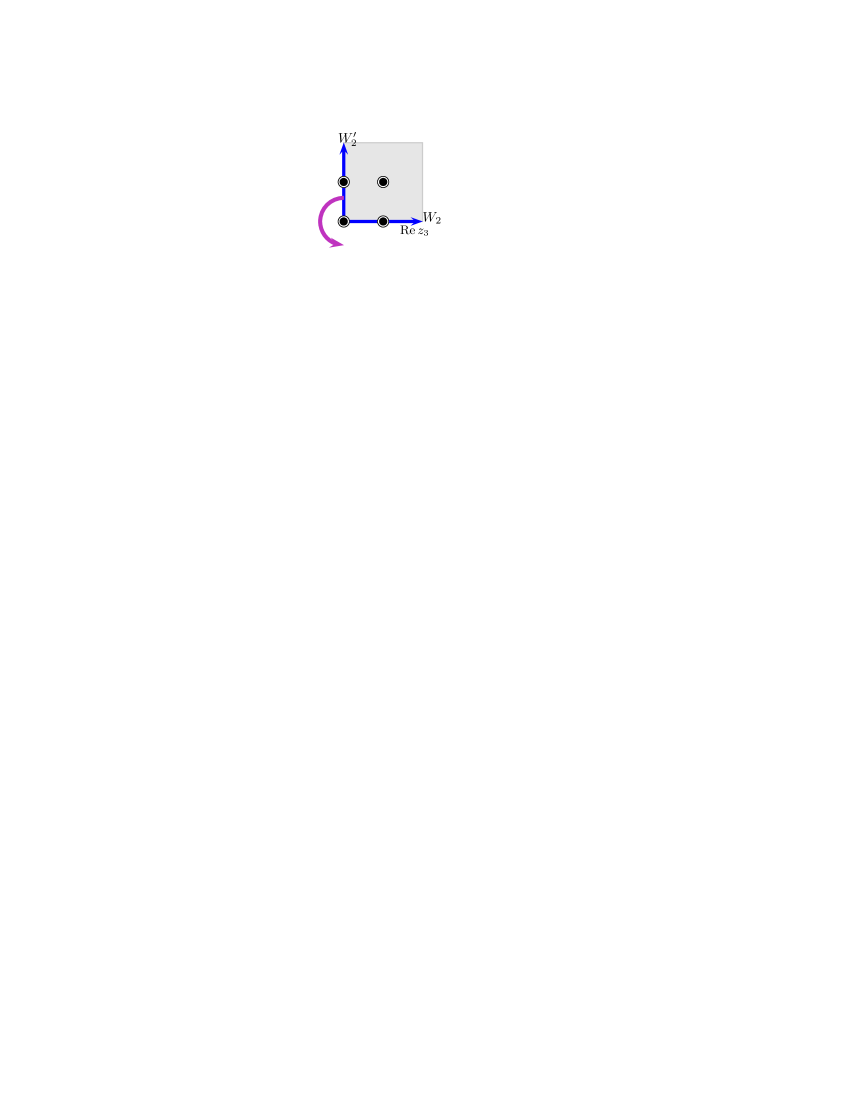
Figure 2: $\mathrm{G}_{2}\times\mathrm{SU}(3)\times\mathrm{SO}(4)$ torus lattice of the $\mathbbm{Z}_{6-\mathrm{II}}$ orbifold. Possible Wilson lines are denoted by $W_{3}$, $W_{2}$ and $W_{2}^{\prime}$.

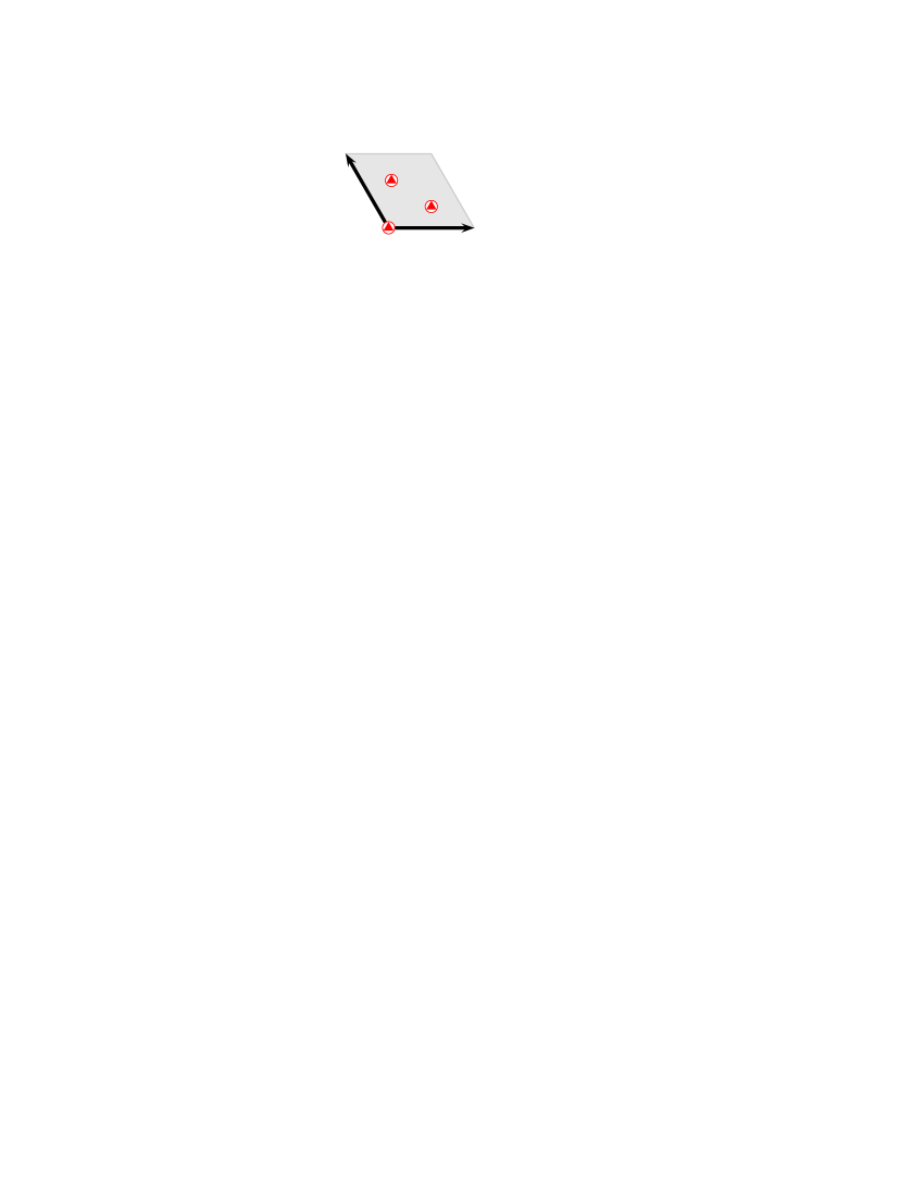
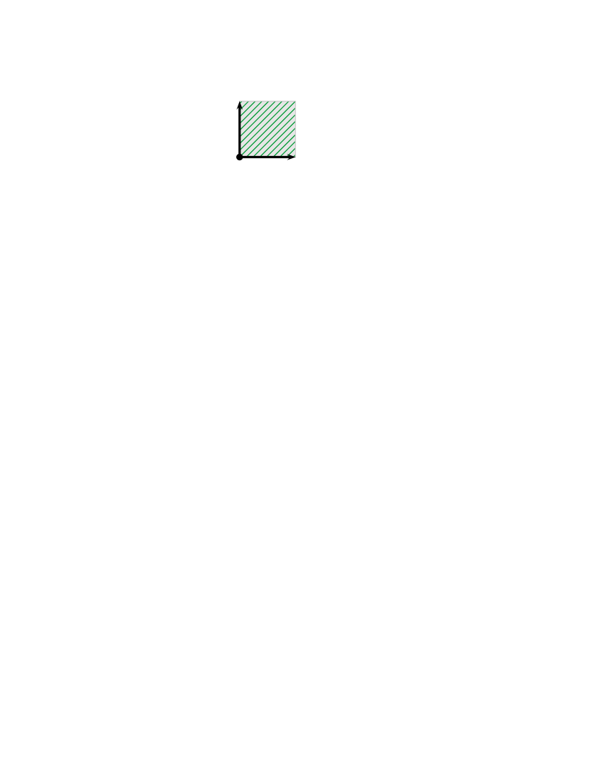
Figure 3: $\mathbbm{Z}_{3}$ fixed points.

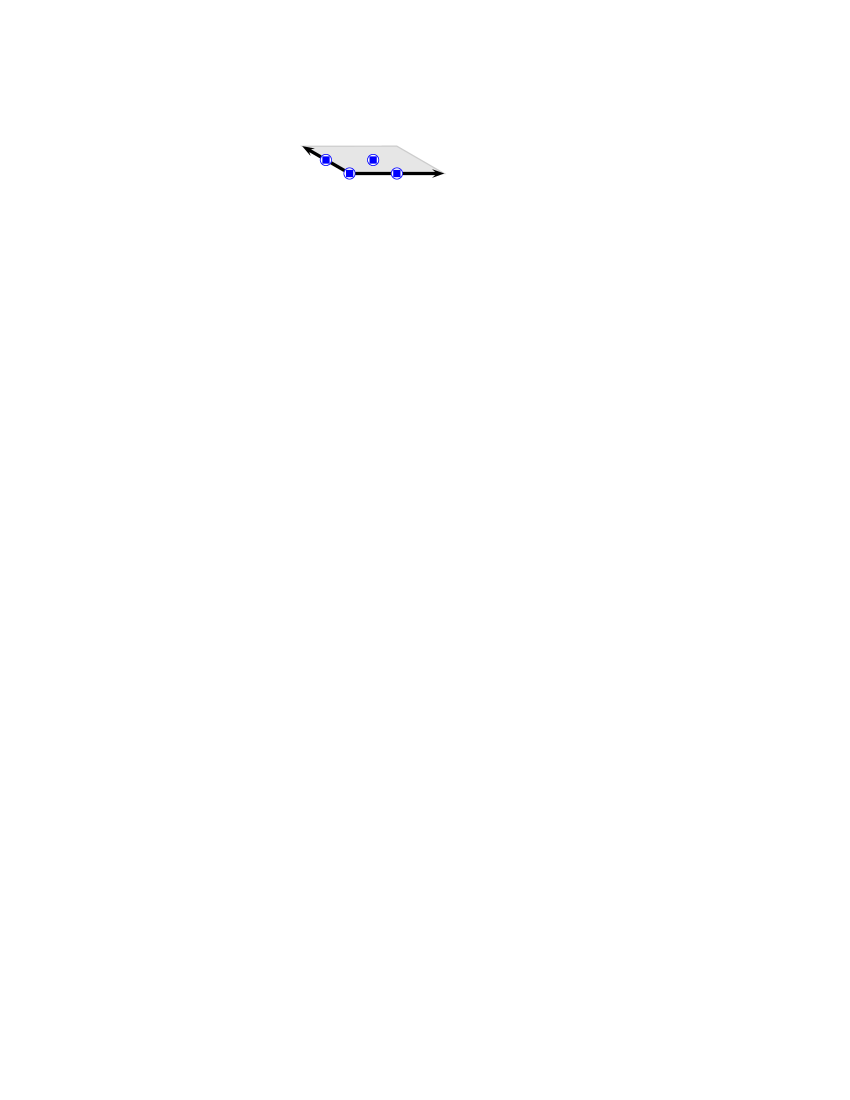
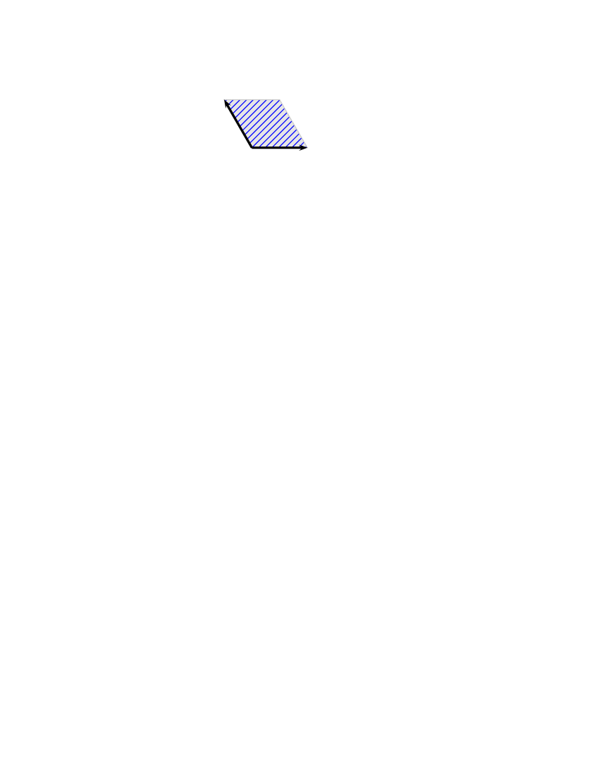
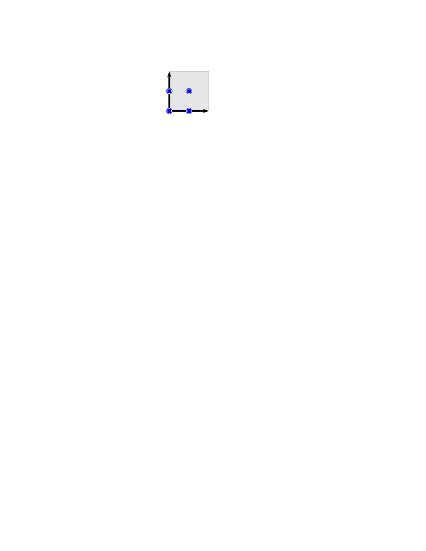
Figure 4: $\mathbbm{Z}_{2}$ fixed points.

The orbifold is flat apart from the singular points (‘conical singularities’) corresponding to the $\mathbbm{Z}_{6}$, $\mathbbm{Z}_{3}$ and $\mathbbm{Z}_{2}$ fixed points. Twisted states are localized at these singularities. In what follows, we detail their localization properties in each $\mathbbm{T}^{2}$ torus.

3.2 Twisted states location

3.2.1 $\boldsymbol{\mathrm{G}_{2}}$ plane

In the $\mathrm{G}_{2}$ plane, there is one point fixed under $\mathbbm{Z}_{6}$ located at the origin, 3 points x,y,z fixed under $\mathbbm{Z}_{3}$, and 4 points a,b,c,d fixed under $\mathbbm{Z}_{2}$ (Fig. 5). Some of them transform into each other under $\mathbbm{Z}_{6}$ twisting and correspond to the same points in the fundamental domain of the orbifold.

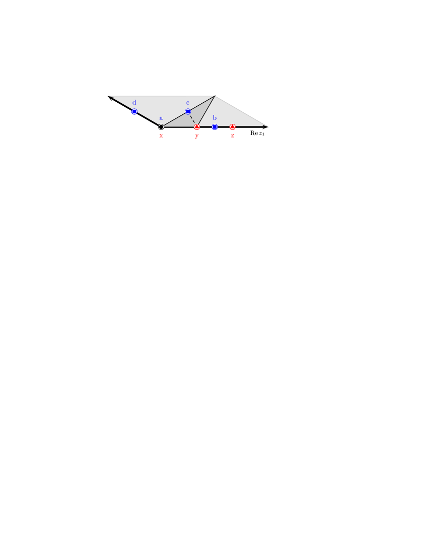
(a) Modding out to the $\mathbbm{Z}_{6}$ ‘pillow’.

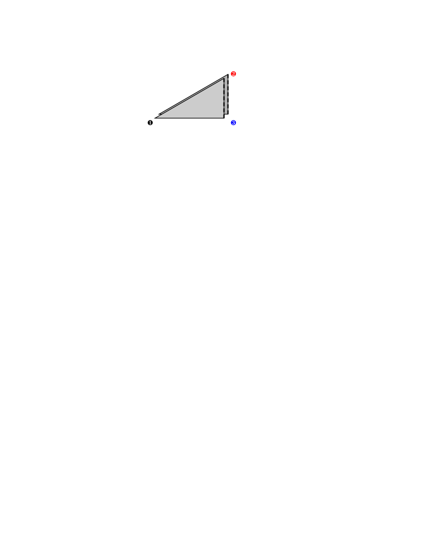
(b) $\mathbbm{Z}_{6}$ ‘pillow’.

Figure 5: The $\mathrm{G}_{2}$ plane. The two simple roots of $\mathrm{G}_{2}$ are given by the arrows in (a) with the shaded area spanned by them being the fundamental region of the torus. The fundamental region of the orbifold is one sixth of this region (darker area) and can be represented by the ‘pillow’ in (b). The latter corresponds to folding the fundamental region along the dashed edge and gluing the other edges together (cf. [45, 46]).

For the three $\mathbbm{Z}_{3}$ fixed points

$$\text{\color[rgb]{1,0,0}x}\equiv\text{\char 182}\;,\quad\text{\color[rgb]{1,0,0}y}\equiv\text{\color[rgb]{1,0,0}\char 183}\;,\quad\text{\color[rgb]{1,0,0}z}\;,$$ (3.4)

one has

$$\text{\color[rgb]{1,0,0}x}\to\text{\color[rgb]{1,0,0}x}\;,\quad\text{\color[rgb]{1,0,0}y}\to\text{\color[rgb]{1,0,0}z}\;,\quad\text{\color[rgb]{1,0,0}z}\to\text{\color[rgb]{1,0,0}y}\;,$$ (3.5)

under the $\mathbbm{Z}_{2}$ twist $\theta^{3}$, and the four $\mathbbm{Z}_{2}$ fixed points

$$\text{\color[rgb]{0,0,1}a}\equiv\text{\char 182}\;,\quad\text{\color[rgb]{0,0,1}b}\;,\quad\text{\color[rgb]{0,0,1}c}\equiv\text{\color[rgb]{0,0,1}\char 184}\;,\quad\text{\color[rgb]{0,0,1}d}\;,$$ (3.6)

transform under the $\mathbbm{Z}_{3}$ twist $\theta^{2}$ as

$$\text{\color[rgb]{0,0,1}a}\to\text{\color[rgb]{0,0,1}a}\;,\quad\text{\color[rgb]{0,0,1}b}\to\text{\color[rgb]{0,0,1}c}\;,\quad\text{\color[rgb]{0,0,1}c}\to\text{\color[rgb]{0,0,1}d}\;,\quad\text{\color[rgb]{0,0,1}d}\to\text{\color[rgb]{0,0,1}b}\;.$$ (3.7)

Thus we have the following mapping from the fundamental domain of the torus to the fundamental domain of the orbifold:

$$\left.\begin{array}[]{c}\text{\color[rgb]{1,0,0}x}\\ {\color[rgb]{0,0,1}\text{a}}\end{array}\right\}\to\text{\char 182}\;,\quad\left.\begin{array}[]{c}\text{\color[rgb]{1,0,0}y}\\ \text{\color[rgb]{1,0,0}z}\end{array}\right\}\to\text{\color[rgb]{1,0,0}\char 183}\;,\quad\left.\begin{array}[]{c}{\color[rgb]{0,0,1}\text{b}}\\ {\color[rgb]{0,0,1}\text{c}}\\ {\color[rgb]{0,0,1}\text{d}}\end{array}\right\}\to\text{\color[rgb]{0,0,1}\char 184}\;.$$ (3.8)

Consequently, $T_{2,4}$ twisted matter lives at ❶ or ❷ points of the orbifold ‘pillow’, whereas $T_{3}$ twisted matter lives at ❶ or ❸.

As explained in Sec. 2.5.2, the fact that the $\mathbbm{Z}_{3}$ and $\mathbbm{Z}_{2}$ fixed points are not fixed under $\mathbbm{Z}_{6}$ introduces a new quantum number for physical states, a phase $\gamma=e^{2\pi\mathrm{i}q_{\gamma}}$ with fractional $q_{\gamma}$. Consider the $T_{2,4}$ twisted sectors. Among the states localized at ❷, there are two linear combinations

$$|\text{\color[rgb]{1,0,0}\char 183};+1\rangle~{}=~{}{1\over\sqrt{2}}\left(|{\color[rgb]{1,0,0}\text{y}}\rangle+|{\color[rgb]{1,0,0}\text{z}}\rangle\right)\;,\quad|\text{\color[rgb]{1,0,0}\char 183};-1\rangle~{}=~{}{1\over\sqrt{2}}\left(|{\color[rgb]{1,0,0}\text{y}}\rangle-|{\color[rgb]{1,0,0}\text{z}}\rangle\right)\;,$$ (3.9)

which are $\mathbbm{Z}_{2}$ (and $\mathbbm{Z}_{6}$) eigenstates with eigenvalues $\gamma=\pm 1$,

$$\theta^{3}\,|\text{\color[rgb]{1,0,0}\char 183};+1\rangle~{}=~{}|\text{\color[rgb]{1,0,0}\char 183};+1\rangle\;,\quad\theta^{3}\,|\text{\color[rgb]{1,0,0}\char 183};-1\rangle~{}=~{}-|\text{\color[rgb]{1,0,0}\char 183};-1\rangle\;.$$ (3.10)

These eigenstates can be labelled by the order of the twist $k=2,4$ and the parameter $q_{\gamma}$,

$$|\text{\color[rgb]{1,0,0}\char 183};+1\rangle~{}=~{}|k=2,4;q_{\gamma}=1\rangle\;,\quad|\text{\color[rgb]{1,0,0}\char 183};-1\rangle~{}=~{}|k=2,4;q_{\gamma}=1/2\rangle\;.$$ (3.11)

The state at the origin has $\gamma=1$ and can be labelled as

$$|\text{\color[rgb]{1,0,0}x}\rangle~{}=~{}|\text{\char 182};+1\rangle~{}=~{}|k=2,4;q_{\gamma}=0\rangle\;.$$ (3.12)

To distinguish $\gamma=1$ states at ❶ from those at ❷, we assign $q_{\gamma}=0$ to the former and $q_{\gamma}=1$ to the latter.

The $T_{3}$ states are treated analogously. There are three linear combinations of states located at ❸, with $\mathbbm{Z}_{3}$ eigenvalues $1$, $\omega\equiv e^{2\pi\mathrm{i}/3}$, and $\omega^{-1}$,

$$|\text{\color[rgb]{0,0,1}\char 184};1\rangle = {1\over\sqrt{3}}\left(|{\color[rgb]{0,0,1}\text{b}}\rangle+|{\color[rgb]{0,0,1}\text{c}}\rangle+|{\color[rgb]{0,0,1}\text{d}}\rangle\right)\;,$$ (3.13a)

$$|\text{\color[rgb]{0,0,1}\char 184};\omega\rangle = {1\over\sqrt{3}}\left(|{\color[rgb]{0,0,1}\text{b}}\rangle+\omega^{-1}|{\color[rgb]{0,0,1}\text{c}}\rangle+\omega^{-2}|{\color[rgb]{0,0,1}\text{d}}\rangle\right)\;,$$ (3.13b)

$$|\text{\color[rgb]{0,0,1}\char 184};\omega^{-1}\rangle = {1\over\sqrt{3}}\left(|{\color[rgb]{0,0,1}\text{b}}\rangle+\omega\,|{\color[rgb]{0,0,1}\text{c}}\rangle+\omega^{2}\,|{\color[rgb]{0,0,1}\text{d}}\rangle\right)\;.$$ (3.13c)

The $\mathbbm{Z}_{3}$ (and $\mathbbm{Z}_{6}$) eigenstates can again be characterized by the order of the twist and $q_{\gamma}$,

$$|\text{\color[rgb]{0,0,1}\char 184};1\rangle~{}=~{}|k=3;q_{\gamma}=1\rangle\;,\quad|\text{\color[rgb]{0,0,1}\char 184};\omega^{\pm 1}\rangle~{}=~{}|k=3;q_{\gamma}=\pm 1/3\rangle\;.$$ (3.14)

The state at the origin is now labelled as

$$|\text{\color[rgb]{0,0,1}a}\rangle~{}=~{}|\text{\char 182};1\rangle~{}=~{}|k=3;q_{\gamma}=0\rangle\;.$$ (3.15)

The $T_{1,5}$ twisted sector states are localized at the origin, which corresponds to a $\mathbbm{Z}_{6}$ eigenstate with eigenvalue $\gamma=1$, i.e.,

$$|\text{\char 182};1\rangle~{}=~{}|k=1,5;q_{\gamma}=0\rangle\;.$$ (3.16)

The location of all $T_{k}$ twisted states is illustrated in Fig. 6.

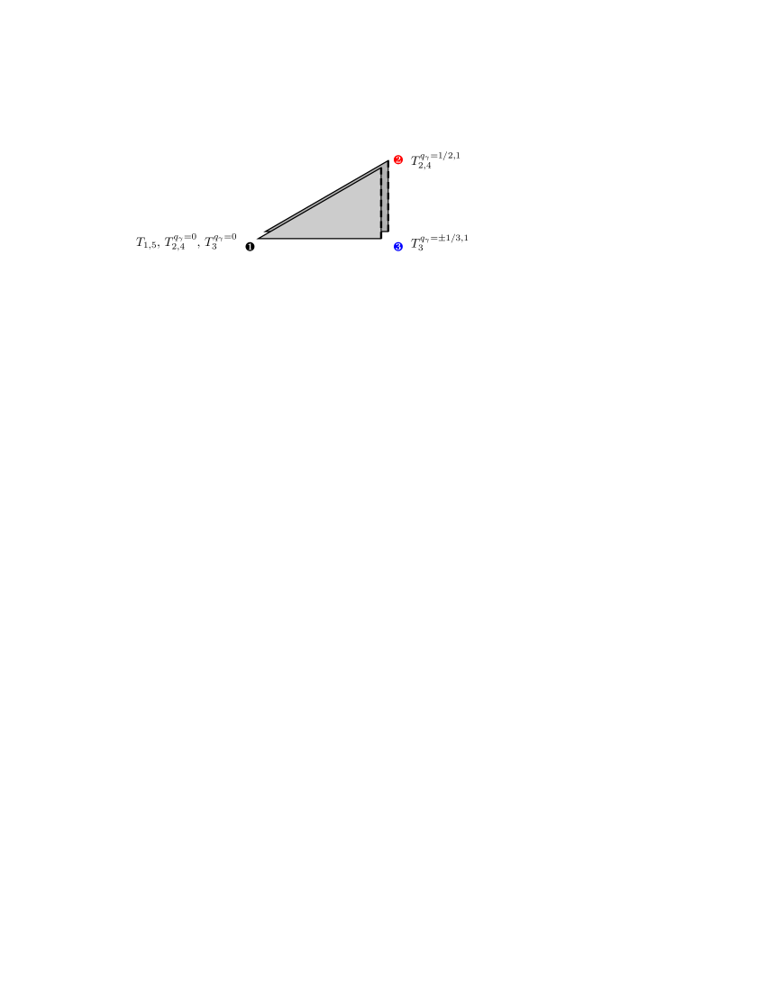
Figure 6: Location of the twisted states in the $\mathrm{G}_{2}$ plane.

The effect of the quantum number $q_{\gamma}$ on the projection conditions for physical states has been discussed in Sec. 2.

3.2.2 $\boldsymbol{\mathrm{SU}(3)}$ plane

States twisted by $\theta^{k}$ with $k=1,2,4,5$ are localized at the three fixed points in the $\mathrm{SU}(3)$ plane, whereas $T_{3}$ and untwisted states live in the bulk. The localization is specified by the quantum number $n_{3}$ (cf. Fig. 7(a)). Tab. 3.1 lists the coordinates of the fixed points in the $\mathrm{SU}(3)$ torus as well as the corresponding space group elements. The coordinates are defined up to translations in the sublattice $2\pi[n\,e_{3}+(-n-3m)\,e_{4}]$ with $n,m\in\mathbbm{Z}$.

$\begin{array}[]{|c|c|cc|cc|cc|}\hline\cr&\text{location}&\vrule\lx@intercol\hfil\text{space group element}\hfil\lx@intercol\vrule\lx@intercol\\ \cline{3-8}\cr n_{3}&\text{(in $2\pi$ units)}&k=1&m_{3}&k=2&m_{3}&k=4&m_{3}\\ \hline\cr 0&0&(\theta,0)&0&(\theta^{2},0)&0&(\theta^{4},0)&0\\ 1&\frac{1}{3}e_{3}+\frac{2}{3}e_{4}&(\theta,e_{3})&1&(\theta^{2},-e_{3})&2&(\theta^{4},e_{3})&1\\ 2&\frac{2}{3}e_{3}+\frac{1}{3}e_{4}&(\theta,-e_{3})&2&(\theta^{2},e_{3})&1&(\theta^{4},-e_{3})&2\\ \hline\cr\end{array}$

Table 3.1: Localization quantum numbers and space group elements.

As discussed in Sec. 2, a fixed point or plane with the space group element $(\theta^{k},a\,e_{3}+b\,e_{4})$ corresponds to the local gauge shift

$$V_{f}~{}=~{}k\,V_{6}+m_{3}\,W_{3}\;,\quad m_{3}~{}=~{}a+b~{}{\rm mod}~{}3\;,$$ (3.17)

up to terms involving $W_{2}$ and $W_{2}^{\prime}$. Note that $m_{3}$ depends not only on the location ($n_{3}$) but also on the order of the twist $k$ (Tab. 3.1). The above local shift is equivalent to

$$V_{f}~{}=~{}k(V_{6}+n_{3}\,W_{3})\;.$$ (3.18)

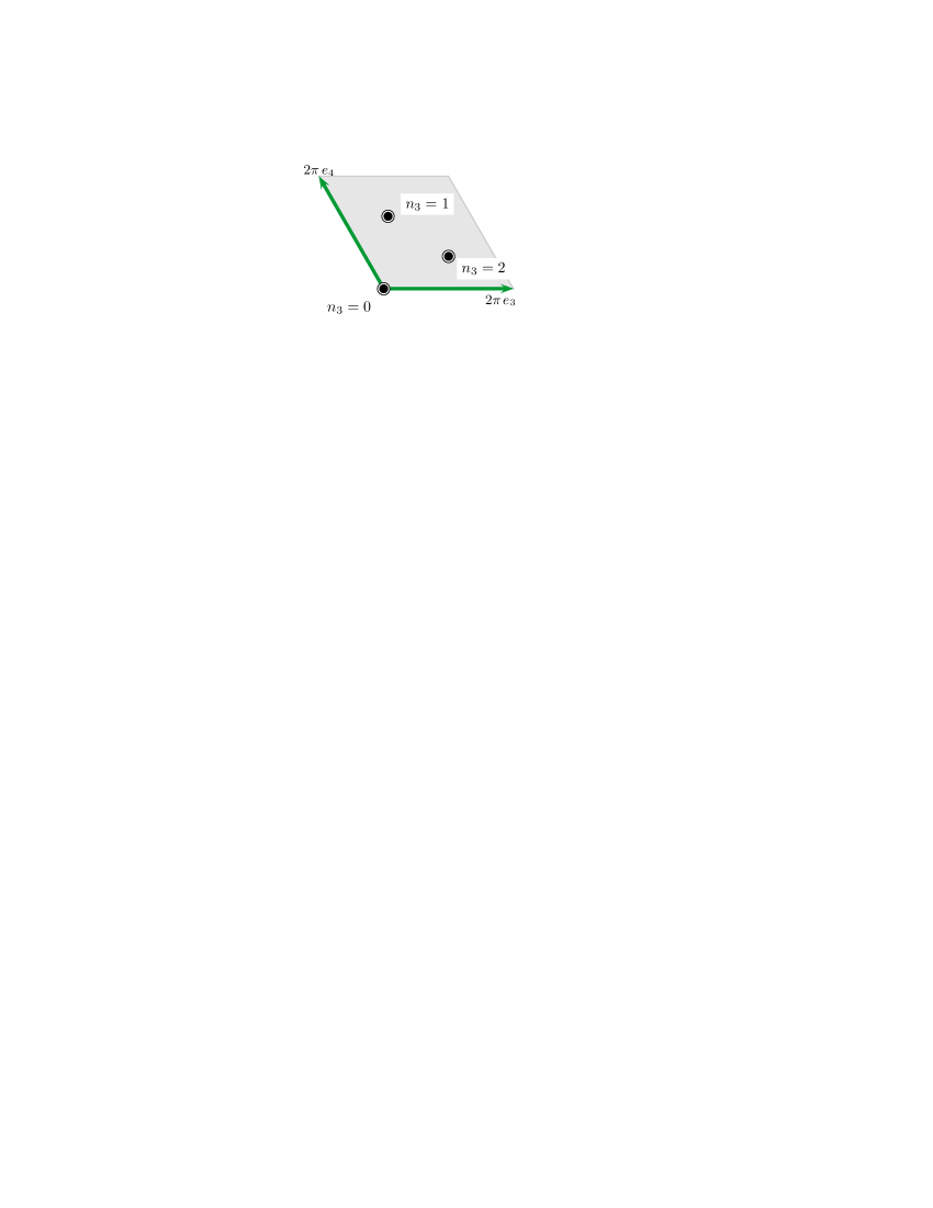
(a) $\mathrm{SU}(3)$ plane.

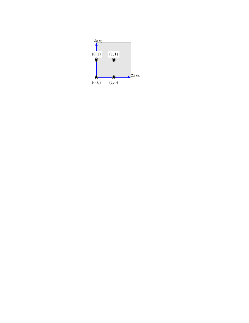
(b) $\mathrm{SO}(4)$ plane.

Figure 7: Localization quantum numbers $n_{3}$, $n_{2}$ and $n_{2}^{\prime}$.

3.2.3 $\boldsymbol{\mathrm{SO}(4)}$ plane

Twisted states from $T_{1,5}$ and $T_{3}$ are localized at the four fixed points in the $\mathrm{SO}(4)$ plane whereas $T_{2}$, $T_{4}$ and untwisted states correspond to bulk fields. The fixed points are labelled by $n_{2}$ and $n_{2}^{\prime}$ (Fig. 7(b)). Tab. 3.2 lists the coordinates of the fixed points and the corresponding space group elements. The coordinates are defined up to translations in the sublattice $2\pi[2n\,e_{5}+2m\,e_{6}]$ where $n,m\in\mathbbm{Z}$. The local shift for the $\theta^{k}$ sectors ($k=1,3,5$) reads

$$V_{f}~{}=~{}k\,(V_{6}+n_{2}\,W_{2}+n_{2}^{\prime}\,W_{2}^{\prime})$$ (3.19)

up to terms involving $W_{3}$.

$\begin{array}[]{|c|c|c|c|}\hline\cr&\text{location}&\vrule\lx@intercol\hfil\text{space group element}\hfil\lx@intercol\vrule\lx@intercol\\ \cline{3-4}\cr(n_{2},n_{2}^{\prime})&\text{(in $2\pi$ units)}&k=1&k=3\\ \hline\cr(0,0)&0&(\theta,0)&(\theta^{3},0)\\ (0,1)&\frac{1}{2}e_{6}&(\theta,e_{6})&(\theta^{3},e_{6})\\ (1,0)&\frac{1}{2}e_{5}&(\theta,e_{5})&(\theta^{3},e_{5})\\ (1,1)&\frac{1}{2}(e_{5}+e_{6})&(\theta,e_{5}+e_{6})&(\theta^{3},e_{5}+e_{6})\\ \hline\cr\end{array}$

Table 3.2: Localization quantum numbers and space group elements.

4 Superpotential

In this section, we discuss the superpotential couplings in heterotic orbifolds. Interactions on orbifolds are calculated using superconformal field theories [47, 43]. This leads to a set of selection rules dictating which couplings are allowed. For our purposes, it suffices to identify the allowed couplings without knowing their precise strength. The following discussion is closely related to the analysis of Kobayashi et al. [22], with some extensions.

4.1 Vertex operators and correlation functions

In orbifold conformal field theory, couplings are obtained from correlation functions of vertex operators for the corresponding physical states. The vertex operators for bosons in the ($-1$)–ghost picture read (cf. [22]):

$$\boldsymbol{V}^{(f)}_{\!\!-1}~{}=~{}e^{-\phi}\,e^{2\mathrm{i}(q+kv_{N})\cdot H}\,e^{2\mathrm{i}(p+V_{f})\cdot X}\prod_{i=1}^{3}\left(\overline{\partial}Z^{i}\right)^{\widetilde{N}_{fi}}\left(\overline{\partial}Z^{*\,i}\right)^{\widetilde{N}^{*}_{fi}}\sigma_{f}\;.$$ (4.1)

Here $q$, $k$, $p$, $f$ and $\widetilde{N}_{fi}$, $\widetilde{N}_{fi}^{*}$ are the quantum numbers described in Sec. 2, and $\sigma_{f}$ is the twist field which creates the vacuum of the twisted sector at the fixed point $f$ from the untwisted vacuum (cf. [47, 43, 49, 50, 51]); $\phi$ is the bosonized superconformal ghost (cf. [52]). Vertex operators for untwisted states correspond to $k=V_{f}=0$, $\sigma_{f}=1$.

In the 0–ghost picture, (4.1) is replaced with

$$\boldsymbol{V}^{(f)}_{\!\!0} = e^{2\mathrm{i}(q+kv_{N})\cdot H}\,e^{2\mathrm{i}(p+V_{f})\cdot X}\,\prod_{i=1}^{3}\left(\overline{\partial}Z^{i}\right)^{\widetilde{N}_{fi}}\left(\overline{\partial}Z^{*\,i}\right)^{\widetilde{N}^{*}_{fi}}$$ (4.2)

$$\hskip 85.35826pt\times\sum_{j=1}^{3}\left(e^{2\mathrm{i}H^{j}}\partial Z^{j}+e^{-2\mathrm{i}H^{j}}\partial Z^{*\,j}\right)\sigma_{f}\;.$$

The vertex operator for fermions is given by

$$\boldsymbol{V}^{(f)}_{\!\!-1/2}~{}=~{}e^{-{\phi\over 2}}\,e^{2\mathrm{i}(q+kv_{N})\cdot H}\,e^{2\mathrm{i}(p+V_{f})\cdot X}\,\prod_{i=1}^{3}\left(\overline{\partial}Z^{i}\right)^{\widetilde{N}_{fi}}\left(\overline{\partial}Z^{*\,i}\right)^{\widetilde{N}^{*}_{fi}}\sigma_{f}\;.$$ (4.3)

In what follows, we will mainly be interested in the superpotential couplings. These are extracted from couplings between 2 fermions and $n-2$ bosons given by the correlation functions

$$\left\langle\boldsymbol{V}^{(f_{1})}_{\!\!-1/2}\,\boldsymbol{V}^{(f_{2})}_{\!\!-1/2}\,\boldsymbol{V}^{(f_{3})}_{\!\!-1}\,\boldsymbol{V}^{(f_{4})}_{\!\!0}\ldots\boldsymbol{V}^{(f_{n})}_{\!\!0}\right\rangle\;.$$ (4.4)

The correlation function (4.4) factorizes into correlators involving separately the fields $\phi$, $H$, $X^{I}$, $Z^{i}$ and the twist fields [47, 43, 49, 50, 51]. $\mathbbm{Z}_{6}$ invariance of each correlator leads to various selection rules which we discuss in the following.

4.2 Selection rules

4.2.1 Gauge invariance

Consider a coupling of $n$ massless physical states labelled by index $r$. As expected, the coupling has to obey gauge invariance. The gauge quantum numbers are specified by the shifted momenta $p+V_{f}$ which play the role of the weight vectors w.r.t. the unbroken subgroup of $\mathrm{E}_{8}\times\mathrm{E}_{8}$. For the correlation function to be non–zero, the states have to form a gauge singlet,

$$\sum_{r=1}^{n}(p+V_{f})_{(r)}~{}=~{}0\;.$$ (4.5)

It is instructive to interpret a coupling among twisted fields in terms of local gauge groups. Suppose that the twisted states form representations $\boldsymbol{R}$, $\boldsymbol{R^{\prime}}$, etc. under the local non–Abelian gauge groups $G_{\mathrm{local}}$, $G_{\mathrm{local}}^{\prime}$, etc. Then the coupling among these states is invariant under the intersection of these groups,

$$G_{\mathrm{intersection}}~{}=~{}G_{\mathrm{local}}\cap G_{\mathrm{local}}^{\prime}\cap G_{\mathrm{local}}^{\prime\prime}\cap\dots~{}\subset~{}\mathrm{E}_{8}\times\mathrm{E}_{8}\;,$$ (4.6)

which is given by the $\mathrm{E}_{8}\times\mathrm{E}_{8}$ roots common to all of the local groups. The remaining gauge invariance conditions concern $\mathrm{U}(1)$ charges. $\boldsymbol{R}$, $\boldsymbol{R^{\prime}}$, etc. can be decomposed into representations of $G_{\mathrm{intersection}}$ such that the invariant couplings involve the latter. This implies, for instance, that a coupling between localized $\boldsymbol{16}$–plets of $\mathrm{SO}(10)$ and other twisted states need not be invariant under the full $\mathrm{SO}(10)$. As a result, a mass term for the SM singlet in the $\boldsymbol{16}$–plet can be written without invoking large $\mathrm{SO}(10)$ representations such as $\boldsymbol{126}$–plets, which are necessary in 4D GUTs.

4.2.2 $\boldsymbol{H}$–momentum rules

Twist invariance of the compact 6D space requires that the superpotential be a scalar with respect to discrete rotations in the compact space. In other words, the $H$–momenta must add up to zero (up to a discrete ambiguity). The $H$–momenta invariant under the ghost picture changing are defined by [22]

$$R^{i}_{(r)}~{}=~{}(q^{i}+kv^{i}_{6})_{(r)}-(\widetilde{N}_{fi}-\widetilde{N}^{*}_{fi})_{(r)}$$ (4.7)

and can be thought of as discrete $R$–charges [49, 53]. They lie on the $\mathrm{SO}(8)$ weight lattice.

For an allowed coupling between 2 fermions and $n-2$ bosons, the sum of the $H$–momenta must vanish. This rule can be reformulated in terms of bosonic $H$–momenta only. Specifically,

$$\sum_{r=1}^{n}R^{1}_{(r)} = -1\mod 6\;,$$ (4.8a)

$$\sum_{r=1}^{n}R^{2}_{(r)} = -1\mod 3\;,$$ (4.8b)

$$\sum_{r=1}^{n}R^{3}_{(r)} = -1\mod 2\;,$$ (4.8c)

where $R^{i}_{(r)}$ are the $H$–momenta of the bosonic components of chiral superfields. For the $\mathbbm{Z}_{6-\mathrm{II}}$ orbifold these are listed in Tab. 4.1.

$k$ $H$–momentum 1 $\frac{1}{6}(-1,-2,-3)$ 2 $\frac{1}{3}(-1,-2,0)$ 3 $\frac{1}{2}(-3,0,-3)$ 4 $\frac{1}{3}(-2,-1,0)$ 5 $\frac{1}{6}\left(-5,-4,-3\right)$

Table 4.1: $\mathbbm{Z}_{6-\mathrm{II}}$ orbifold: $H$–momenta for bosons containing no oscillators.

We note that gauge invariance requires strict vanishing of the sum of $\mathrm{E}_{8}\times\mathrm{E}_{8}$ momenta, whereas the sum of $H$–momenta must vanish up to a discrete shift as given above. The difference between the two rules stems from the fact that the gauge 16D torus possesses continuous symmetries, while in the case of the 6D orbifold they are only discrete.

4.2.3 Space group selection rules

The space group selection rule [47, 43] states that the string boundary conditions have to match in order for the coupling to be allowed. Consider twisted states living at the fixed points $f_{1}$, $f_{2}$,…$f_{n}$ corresponding to the space group elements $(\theta^{k_{(1)}},\ell_{(1)})$, $(\theta^{k_{(2)}},\ell_{(2)})$, …, $(\theta^{k_{(n)}},\ell_{(n)})$. A coupling of these states is allowed if (cf. [49])

$$(\theta^{k_{(1)}},\ell_{(1)})\,(\theta^{k_{(2)}},\ell_{(2)})\dots(\theta^{k_{(n)}},\ell_{(n)})~{}=~{}(\mathbbm{1},0)$$ (4.9)

up to a torus lattice vector $\sum_{r=1}^{n}\Lambda_{k_{(r)}}$, where $\Lambda_{k_{(r)}}=(\mathbbm{1}-\theta^{k_{(r)}})\Lambda$. The untwisted sector corresponds to the space group element $(\mathbbm{1},0)$. The above condition is equivalent to (cf. App. B)

$$\sum\limits_{r=1}^{n}k_{(r)} = 0\mod 6\;,$$ (4.10a)

$$\sum\limits_{r=1}^{n}\ell_{(r)} = 0\mod{\sum_{r=1}^{n}\Lambda_{k_{(r)}}}\;.$$ (4.10b)

The first equation restricts the twisted sectors that can couple and states that the total twist of the coupling must be $0\mod 6$. The second condition puts a restriction on the fixed points. In terms of the localization quantum numbers, it reads

$$\mathrm{SU}(3) : \sum\limits_{r=1}^{n}k_{(r)}\,n_{3(r)}~{}=~{}0\mod 3\;,$$ plane (4.11a)

$$\mathrm{SO}(4) : \sum\limits_{r=1}^{n}n_{2(r)}~{}=~{}0\mod 2\;,$$ plane (4.11c)

$$\sum\limits_{r=1}^{n}n^{\prime}_{2(r)}~{}=~{}0\mod 2\;,$$

plus an additional condition to be discussed below. The quantum numbers $n_{3(r)}$, $n_{2(r)}$ and $n^{\prime}_{2(r)}$ have been defined in Sec. 3. The space group selection rule for the $\mathrm{SU}(3)$ plane is illustrated in Fig. 8.

(a) Allowed.

(b) Allowed.

(c) Forbidden.

Figure 8: Allowed (a,b) and forbidden (c) 3–point couplings between localized states $|A\rangle,|B\rangle,|C\rangle$ in the $\mathrm{SU}(3)$ plane.

For the $\mathrm{G}_{2}$ plane, there is a non–trivial selection rule if only $T_{2}$ and $T_{4}$, or only $T_{3}$ states are involved in the coupling. As we show in App. B, the coupling must satisfy

$$\{q_{\gamma(1)},\dots q_{\gamma(n)}\}~{}\not\in~{}\text{permutations}\{x,0,\dots 0\}\;$$ (4.12)

for $x\not=0$.

To summarize, we have presented the string selection rules which determine whether a given superpotential coupling is allowed. Apart from gauge invariance, such couplings enjoy certain discrete symmetries related to the localization properties of the states involved.

5 The MSSM from the heterotic string

In this section, we present an orbifold compactification of the $\mathrm{E}_{8}\times\mathrm{E}_{8}$ heterotic string which yields the MSSM spectrum and gauge group at low energies. Apart from the MSSM sector, the model contains a hidden sector which can account for low–energy supersymmetry breakdown. In this section we present basic features of the model, whereas other important aspects such as vacuum configurations, SUSY breaking, and phenomenology will be discussed in Secs. 6–8.

5.1 Search Strategy

It is well known that with an appropriate choice of the gauge shift $V$ and Wilson lines, it is not difficult to get the standard model gauge group times extra group factors. The real challenge however is to get three generations of the SM matter.

We base our search on the concept of local GUTs. Since one complete matter generation (plus a right–handed neutrino) is a $\boldsymbol{16}$–plet of $\mathrm{SO}(10)$, we use the gauge shifts which admit local $\mathrm{SO}(10)$ symmetry and $\boldsymbol{16}$–plets at the fixed points. There are only two such shifts in a $\mathbbm{Z}_{6-\mathrm{II}}$ orbifold [54, 55],

$$V_{6} = \left(\frac{1}{2},\frac{1}{2},\frac{1}{3},0,0,0,0,0\right)\,\left(\frac{1}{3},0,0,0,0,0,0,0\right)\;,$$

$$V_{6}^{\prime} = \left(\frac{1}{3},\frac{1}{3},\frac{1}{3},0,0,0,0,0\right)\,\left(\frac{1}{6},\frac{1}{6},0,0,0,0,0,0\right)\;.$$ (5.1)

Each of them ensures that there are $\boldsymbol{16}$–plets in the $T_{1}$ sector, which remain in the massless spectrum regardless of the Wilson lines. Further, one adjusts the Wilson lines such that the gauge group in 4D is that of the standard model times additional factors.

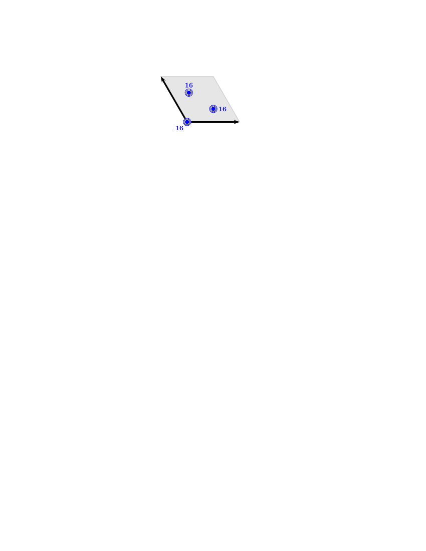
(a)

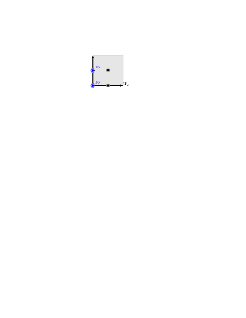
(b)

Figure 9: 3 vs. $2$ equivalent families.

To obtain three matter generations, the simplest option is to use three equivalent fixed points with local $\mathrm{SO}(10)$ symmetry [23], Fig. 9(a). This would provide an intuitive explanation for triplication of fermion families. However, our scan over such models shows that in this case there are always chiral exotic states in the spectrum (cf. App. C). Such states get masses due to electroweak symmetry breaking and generally are inconsistent with experiment. A similar statement applies to other $\mathbbm{Z}_{n}$ orbifolds with $n\leq 6$.

This result implies that the three families of $\boldsymbol{16}$–plets are not all equivalent, at least in the context of $\mathbbm{Z}_{\leq 6}$ orbifold models. We are thus led to consider the next–to–simplest possibility: 2 equivalent families and one different family, Fig. 9(b). The equivalent $\boldsymbol{16}$–plets can appear due to 2 equivalent fixed points in the SO(4) plane with one Wilson line $W_{2}$. The remaining family then has to come from other sectors of the model. We find that this procedure is successful and, in many cases, the exotic matter is vector–like with respect to the standard model. Furthermore, we find that the vector–like matter can be consistently decoupled at least in one case.

5.2 The model

Our model is a $\mathbbm{Z}_{6-\mathrm{II}}$ heterotic orbifold based on the Lie lattice $\mathrm{G}_{2}\times\mathrm{SU}(3)\times\mathrm{SO}(4)$. It involves two Wilson lines: one of order 2, $W_{2}$, and another of order 3, $W_{3}$, and has the gauge shift $V_{6}$ consistent with the local SO(10) structure. Specifically, the gauge shift and the Wilson lines are given by [26]

$$V_{6} = \left(\frac{1}{2},\frac{1}{2},\frac{1}{3},0,0,0,0,0\right)\,\left(\frac{1}{3},0,0,0,0,0,0,0\right)\;,$$

$$W_{2} = \left(\frac{1}{2},0,\frac{1}{2},\frac{1}{2},\frac{1}{2},0,0,0\right)\,\left(-\frac{3}{4},\frac{1}{4},\frac{1}{4},-\frac{1}{4},\frac{1}{4},\frac{1}{4},\frac{1}{4},-\frac{1}{4}\right)\;,$$

$$W_{3} = \left(\frac{1}{3},0,0,\frac{1}{3},\frac{1}{3},\frac{1}{3},\frac{1}{3},\frac{1}{3}\right)\,\left(1,\frac{1}{3},\frac{1}{3},\frac{1}{3},0,0,0,0\right)\;.$$ (5.2)

By adding elements of the root lattice $\Lambda_{\mathrm{E}_{8}\times\mathrm{E}_{8}}$ to the shift and Wilson lines, one can transform this set to

$$V_{6}^{\prime} = \left(-\frac{1}{2},-\frac{1}{2},\frac{1}{3},0,0,0,0,0\right)\,\left(\frac{17}{6},-\frac{5}{2},-\frac{5}{2},-\frac{5}{2},-\frac{5}{2},-\frac{5}{2},-\frac{5}{2},\frac{5}{2}\right)\;,$$

$$W_{2}^{\prime} = \left(-\frac{1}{2},0,-\frac{1}{2},\frac{1}{2},\frac{1}{2},0,0,0\right)\,\left(\frac{23}{4},-\frac{25}{4},-\frac{21}{4},-\frac{19}{4},-\frac{25}{4},-\frac{21}{4},-\frac{17}{4},\frac{17}{4}\right)\;,$$

$$W_{3}^{\prime} = \left(-\frac{1}{6},\frac{1}{2},\frac{1}{2},-\frac{1}{6},-\frac{1}{6},-\frac{1}{6},-\frac{1}{6},-\frac{1}{6}\right)\,\left(0,-\frac{2}{3},\frac{1}{3},\frac{4}{3},-1,0,0,0\right)\;,$$ (5.3)

which fulfills the ‘strong’ modular invariance conditions (2.30).

The gauge group after compactification is

$$G~{}=~{}\mathrm{SU}(3)\times\mathrm{SU}(2)\times[\mathrm{SU}(4)\times\mathrm{SU}(2)^{\prime}]\times\mathrm{U}(1)^{9}\;.$$ (5.4)

Here the brackets $[\dots]$ indicate a subgroup of the second $\mathrm{E}_{8}$ factor. The generators of the $\mathrm{U}(1)$ factors can be chosen as

$$\mathsf{t}_{1} = \mathsf{t}_{Y}~{}=~{}\left(0,0,0,\frac{1}{2},\frac{1}{2},-\frac{1}{3},-\frac{1}{3},-\frac{1}{3}\right)\,(0,0,0,0,0,0,0,0)\;,$$

$$\mathsf{t}_{2} = (1,0,0,0,0,0,0,0)\,(0,0,0,0,0,0,0,0)\;,$$

$$\mathsf{t}_{3} = (0,1,0,0,0,0,0,0)\,(0,0,0,0,0,0,0,0)\;,$$

$$\mathsf{t}_{4} = (0,0,1,0,0,0,0,0)\,(0,0,0,0,0,0,0,0)\;,$$

$$\mathsf{t}_{5} = (0,0,0,1,1,1,1,1)\,(0,0,0,0,0,0,0,0)\;,$$

$$\mathsf{t}_{6} = (0,0,0,0,0,0,0,0)\,(1,0,0,0,0,0,0,0)\;,$$

$$\mathsf{t}_{7} = (0,0,0,0,0,0,0,0)\,(0,1,1,0,0,0,0,0)\;,$$

$$\mathsf{t}_{8} = (0,0,0,0,0,0,0,0)\,(0,0,0,1,0,0,0,0)\;,$$

$$\mathsf{t}_{9} = (0,0,0,0,0,0,0,0)\,(0,0,0,0,-1,-1,-1,1)\;.$$ (5.5)

One of the $\mathrm{U}(1)$ factors is ‘anomalous’. It is generated by

$$\mathsf{t}_{\mathrm{anom}}~{}=~{}\sum\limits_{i=1}^{8}c_{i}\,\mathsf{t}_{i}\quad\text{with}\quad c_{i}=\left(0,\frac{11}{6},\frac{1}{2},-\frac{3}{2},-\frac{1}{6},1,\frac{1}{3},\frac{1}{3},0\right)\;.$$ (5.6)

The sum of the anomalous $\mathrm{U}(1)$ charges is

$$\operatorname{tr}\mathsf{t}_{\mathrm{anom}}~{}=~{}88\;,$$ (5.7)

which is relevant to the calculation of the Fayet–Iliopoulos term.

The factors $\mathrm{SU}(3)$ and $\mathrm{SU}(2)$ in $G$ are identified with the color $\mathrm{SU}(3)_{c}$ and the weak $\mathrm{SU}(2)_{\mathrm{L}}$ of the standard model. The hypercharge generator is given by $\mathsf{t}_{Y}$. It is embedded in SO(10) just like in usual 4D GUTs,

$$\mathrm{SU}(3)_{c}\times\mathrm{SU}(2)_{\mathrm{L}}\times\mathrm{U}(1)_{Y}~{}\subset~{}\mathrm{SO}(10)\;.$$ (5.8)

Thus it automatically has the correct normalization and is consistent with gauge coupling unification. It is also important that this hypercharge is non–anomalous, $\mathsf{t}_{Y}\cdot\mathsf{t}_{\mathrm{anom}}=0$.

The massless matter states are listed in Tab. 5.1. They appear in both the untwisted and twisted sectors, apart from $T_{5}$ which has no left–chiral superfields. The spectrum can be summarized as follows:

$$\text{matter:}~{}~{}~{}~{}3\times\boldsymbol{16}~{}~{}+~{}~{}\text{vector-like}\;.$$ (5.9)

Two generations are localized in the compactified space and come from the first twisted sector $T_{1}$, whereas the third generation is partially twisted and partially untwisted:

$$2\times\boldsymbol{16}\in T_{1}~{}~{},~{}~{}\boldsymbol{16}\in U,T_{2},T_{4}\;.$$ (5.10)

In particular, the up–quark and the quark doublet of the third generation are untwisted, which results in a large Yukawa coupling, whereas the down–quark is twisted and its Yukawa coupling is suppressed. The $\boldsymbol{16}$–plet quantum numbers of the third generation are not enforced by local GUTs, but are related to the standard model anomaly cancellation.

Apart from the 3 matter families, the model contains extra states which are vector–like with respect to the standard model gauge group. These include a pair of Higgs doublets and additional exotic matter which, as we show in the subsequent sections, can be consistently decoupled. A complete list of quantum numbers of the massless states is given in Tabs. LABEL:tab:LongTableNonSingletsSaturdayAfternoonModel and LABEL:tab:LongTableSingletsSaturdayAfternoonModel.

name	irrep	count		name	irrep	count
$q_{i}$	$(\boldsymbol{3},\boldsymbol{2};\boldsymbol{1},\boldsymbol{1})_{1/6}$	3		$\bar{u}_{i}$	$(\overline{\boldsymbol{3}},\boldsymbol{1};\boldsymbol{1},\boldsymbol{1})_{-2/3}$	3
$\bar{d}_{i}$	$(\overline{\boldsymbol{3}},\boldsymbol{1};\boldsymbol{1},\boldsymbol{1})_{1/3}$	7		$d_{i}$	$(\boldsymbol{3},\boldsymbol{1};\boldsymbol{1},\boldsymbol{1})_{-1/3}$	4
$\bar{\ell}_{i}$	$(\boldsymbol{1},\boldsymbol{2};\boldsymbol{1},\boldsymbol{1})_{1/2}$	5		$\ell_{i}$	$(\boldsymbol{1},\boldsymbol{2};\boldsymbol{1},\boldsymbol{1})_{-1/2}$	8
$m_{i}$	$(\boldsymbol{1},\boldsymbol{2};\boldsymbol{1},\boldsymbol{1})_{0}$	8		$\bar{e}_{i}$	$(\boldsymbol{1},\boldsymbol{1};\boldsymbol{1},\boldsymbol{1})_{1}$	3
$s^{-}_{i}$	$(\boldsymbol{1},\boldsymbol{1};\boldsymbol{1},\boldsymbol{1})_{-1/2}$	16		$s^{+}_{i}$	$(\boldsymbol{1},\boldsymbol{1};\boldsymbol{1},\boldsymbol{1})_{1/2}$	16
${s}_{i}$	$(\boldsymbol{1},\boldsymbol{1};\boldsymbol{1},\boldsymbol{1})_{0}$	69		$h_{i}$	$(\boldsymbol{1},\boldsymbol{1};\boldsymbol{1},\boldsymbol{2})_{0}$	14
$f_{i}$	$(\boldsymbol{1},\boldsymbol{1};\boldsymbol{4},\boldsymbol{1})_{0}$	4		$\bar{f}_{i}$	$(\boldsymbol{1},\boldsymbol{1};\overline{\boldsymbol{4}},\boldsymbol{1})_{0}$	4
$w_{i}$	$(\boldsymbol{1},\boldsymbol{1};\boldsymbol{6},\boldsymbol{1})_{0}$	5

Table 5.1: Quantum numbers of the massless states w.r.t. $G_{\mathrm{SM}}\times[\mathrm{SU}(4)\times\mathrm{SU}(2)]$ and a field naming convention.

5.3 Local GUT representations

The matter states of the model can be viewed as originating from representations of local GUTs supported at certain fixed points or planes. States from the first twisted sector correspond to ‘brane’ fields living at the orbifold fixed points. As discussed in Sec. 2, such states are invariant under the orbifold action. Thus they all survive in 4D and furnish complete representations of the local GUTs. On the other hand, states from higher twisted (as well as untwisted) sectors are not automatically invariant under the orbifold action. Part of the GUT multiplet is projected out such that the surviving states produce incomplete (‘split’) multiplets in 4D. In particular, the gauge multiplets of $\mathrm{E}_{8}$ reduce to those of the standard model (and extra group factors). The latter can be viewed as an intersection of local GUTs at various orbifold fixed points (see e.g. [25]). We survey the local GUTs and their representations in Tab. LABEL:tab:LocalGUTs.

5.4 Spontaneous gauge symmetry breaking

The effective low energy theory of our orbifold model has, in general, smaller gauge symmetry and fewer massless states than those in Eq. (5.4) and Tab. 5.1. One of the reasons is that there is an anomalous $\mathrm{U}(1)$ which induces a FI $D$–term,

$$D_{\mathrm{anom}}~{}=~{}\sum q_{\mathrm{anom}}^{(i)}\,|\phi_{i}|^{2}+\frac{g\,M_{\mathrm{P}}^{2}}{192\pi^{2}}~{}{\operatorname{tr}\mathsf{t}_{\mathrm{anom}}}\;,$$ (5.11)

where the sum runs over all scalars $\phi_{i}$ with anomalous charges $q_{\mathrm{anom}}^{(i)}$. This $D$–term must be zero in a supersymmetric vacuum, so at least some of the scalars are forced to attain large vacuum expectation values, typically not far below the string scale. As a result, the anomalous $\mathrm{U}(1)$ gets broken. Generically, this also triggers breakdown of other gauge symmetries, under which the above mentioned scalars are charged. The resulting gauge group and matter fields at low energies are therefore a subset of those in Eq. (5.4) and Tab. 5.1.

More generally, some of the scalars can attain VEVs as long as it is consistent with supersymmetry, $F_{i}=D_{a}=0$. In the simplest case, such scalars are associated with flat directions in the field space. In general, supersymmetric configurations are described by non–trivial solutions of $F_{i}=D_{a}=0$, which correspond to points or low–dimensional manifolds in the field space. In either case, this breaks part of the gauge symmetry,

$$G~{}\xrightarrow{\mathrm{VEVs}}~{}G_{\mathrm{low-energy}}\;.$$ (5.12)

Furthermore, such VEVs provide mass terms for some of the matter states. In particular, if the superpotential coupling

$$\Delta W=x_{i}\,\bar{x}_{j}\times\langle s_{\alpha_{1}}...s_{\alpha_{n}}\rangle$$ (5.13)

exists, with $x_{i}$ and $\bar{x}_{j}$ being vector-like states w.r.t. $G_{\mathrm{low-energy}}$ and $s_{\alpha_{k}}$ being the scalars attaining VEVs, then $x_{i}$ and $\bar{x}_{j}$ become massive and decouple from the low energy theory.

It is common that orbifold models contain states which are charged under both $G_{\mathrm{SM}}$ and other gauge factors originating from the second $\mathrm{E}_{8}$. As long as such gauge factors are unbroken, there is no hidden sector in the model, which is usually required for spontaneous SUSY breaking. The separation between the “visible” and the “hidden” comes about when some of the scalars attain VEVs thereby breaking the unwanted gauge factors. In our model, this occurs, in particular, when some of the 69 $s_{i}$ states break $\mathrm{U}(1)^{8}$.

An interesting property of the model is that none of the oscillator states is charged under $G_{\mathrm{SM}}$ (cf. Tabs. LABEL:tab:LongTableNonSingletsSaturdayAfternoonModel, LABEL:tab:LongTableSingletsSaturdayAfternoonModel). If all the oscillators develop VEVs, the unbroken gauge group is $G_{\mathrm{SM}}\times[\mathrm{SU}(4)\times\mathrm{U}(1)]$, while the SM matter is neutral under the additional $\mathrm{U}(1)$. This might be important as it has been argued that giving VEVs to oscillator modes corresponds to resolving the conical singularities associated with the fixed points [49]. This means that the phenomenologically relevant gauge group survives the naive ‘blowing–up’ procedure.

Orbifold models with the same gauge shifts and Wilson lines but different scalar VEVs lead to distinct low–energy theories. For example, in some of them, the standard model gauge group is broken. To obtain realistic models, one has to make sure that, first of all,

• $G_{\mathrm{SM}}$ is unbroken,

• exotic matter is heavy.

There are also further phenomenological constraints which we discuss in the subsequent sections.

5.5 Decoupling the exotic states

A necessary condition for the decoupling of vector–like exotic states, without breaking the standard model gauge group, is the existence of the superpotential couplings

$$x_{i}\,\bar{x}_{j}\,\times(\text{SM singlets})\;.$$ (5.14)

Furthermore, the rank of the $x_{i},\;\bar{x}_{j}$ mass matrix must be maximal such that no massless vector–like states survive. We find that in our model the required mass terms are allowed and the exotic states can be decoupled.

The exotic states charged under $G_{\mathrm{SM}}$ are pairs of $d_{i}$ and $\bar{d}_{i}$, $\ell_{i}$ and $\bar{\ell}_{i}$, $s_{i}^{-}$ and $s_{i}^{+}$, and $m_{i}$. The mass terms for these states have the form

$$W_{\mathrm{mass}}~{}=~{}d_{i}\,\mathcal{M}_{d}^{ij}(s)\,\bar{d}_{j}+\bar{\ell}_{i}\,\mathcal{M}_{\ell}^{ij}(s)\,\ell_{j}+m_{i}\,\mathcal{M}_{m}^{ij}(s)\,m_{j}+s^{+}_{i}\,\mathcal{M}_{s}^{ij}(s)\,s^{-}_{j}\;,$$ (5.15)

where $s$ denotes some SM singlets. Taking $s=\{s_{i}\}$, we find

$$\mathcal{M}_{d}^{ij}(s) = \left(\begin{array}[]{ccccccc}s^{5}&s^{5}&s^{5}&s^{5}&s^{5}&s^{3}&s^{3}\\ s^{1}&s^{1}&s^{3}&s^{3}&s^{3}&s^{3}&s^{3}\\ s^{1}&s^{1}&s^{3}&s^{3}&s^{3}&s^{3}&s^{3}\\ s^{6}&s^{6}&s^{6}&s^{3}&s^{3}&s^{6}&s^{6}\end{array}\right)\;,$$ (5.20)

$$\mathcal{M}_{\ell}^{ij}(s) = \left(\begin{array}[]{cccccccc}s^{3}&s^{4}&s^{4}&s^{1}&s^{1}&s^{1}&s^{1}&s^{1}\\ s^{1}&s^{2}&s^{2}&s^{5}&s^{5}&s^{3}&s^{3}&s^{3}\\ s^{1}&s^{2}&s^{2}&s^{5}&s^{5}&s^{3}&s^{3}&s^{3}\\ s^{1}&s^{2}&s^{2}&s^{5}&s^{5}&s^{6}&s^{3}&s^{3}\\ s^{1}&s^{6}&s^{6}&s^{3}&s^{3}&s^{6}&s^{3}&s^{3}\end{array}\right)\;.$$ (5.26)

$\mathcal{M}_{m}^{ij}(s)$ and $\mathcal{M}_{s}^{ij}(s)$ are given in Eqs. (D.9) and (LABEL:eq:Ms(s)) in App. D, respectively. Here, an entry $s^{N}$ indicates the existence of a coupling which involves $N$ singlets. For instance, the $(1,1)$ entry of the $d$-$\bar{d}$ mass term includes

$$W_{d_{1}\bar{d}_{1}}~{}=~{}d_{1}\bar{d}_{1}(s_{3}s_{20}s_{39}s_{44}s_{65}+s_{7}s_{34}s_{35}s_{40}s_{41}+\cdots)\;,$$ (5.27)

where the coefficients are omitted. Different entries generally involve different combinations of the singlets as well as different couplings, such that the rank of each mass matrix is maximal. We note that higher $N$ does not necessarily imply significant suppression of the coupling [56]: $s$ can be close to the string scale and, furthermore, the coefficient in front of the coupling grows with $N$. We find that all mass matrices have maximal rank at order 8. A zero in the mass matrices (D.9)–(D.32) of App. D.4 indicates that up to order 8 no coupling appears.

This result implies that all of the exotic states can be decoupled below the GUT scale or so. In particular, the rank of $\mathcal{M}_{d}$ is 4 such that only 3 down–type quarks survive. $\mathcal{M}_{\ell}$ has, in general, rank 5 resulting in 3 massless doublets of hypercharge $-1/2$. In order to get an extra pair of (“Higgs”) doublets with hypercharge $-1/2$ and $1/2$, one has to adjust the singlet VEVs such that the rank reduces to 4. This large finetuning constitutes the well known supersymmetric $\mu$–problem and will be discussed in subsequent sections. A further constraint on the above texture comes from the top Yukawa coupling: it is order one if the up–type Higgs doublet has a significant component of $\bar{\ell}_{1}$.

In the above mass matrices, $s$ are chosen to be singlets under $\mathrm{SU}(4)\times\mathrm{SU}(2)^{\prime}$ such that their VEVs break

$$G~{}\longrightarrow~{}\mathrm{SU}(3)_{c}\times\mathrm{SU}(2)_{\mathrm{L}}\times\mathrm{U}(1)_{Y}\times G_{\mathrm{hidden}}\;,$$ (5.28)

with $G_{\mathrm{hidden}}=\mathrm{SU}(4)\times\mathrm{SU}(2)^{\prime}$. Now the model has a truly hidden sector which can be responsible for spontaneous SUSY breaking.

In the next section we show that the required configurations of the singlet VEVs are in general consistent with supersymmetry, e.g. $F_{i}=D_{a}=0$. The $D$–flatness is ensured by constructing gauge invariant monomials out of the singlets [57, 58] involved in the mass terms for the exotic states. We further show that generally there exist non–trivial solutions to $F_{i}=D_{a}=0$ in the form of low–dimensional manifolds in the field space.

Not all vacuum configurations consistent with supersymmetry and the decoupling are phenomenologically viable. Further important constraints are due to

• absence of rapid proton decay,

• realistic flavour structures,

• small $\mu$–term.

This strongly restricts allowed VEVs for the singlets. As we show in Sec. 8, these constraints motivate certain patterns of the VEVs, in particular those which preserve $B\!-\!L$ symmetry at the GUT scale.

Finally, let us remark on gauge invariance of the couplings in the framework of local GUTs. As stated in Eq. (4.6), a coupling among twisted states is invariant under the intersection of local gauge groups supported at the corresponding fixed points, but not necessarily under each of the groups. To give an example, consider an allowed coupling $s_{4}\,s_{26}\,s_{57}$. Each of these singlets originates from a larger representation of the local group. The above coupling arises from the coupling of states contained in $(\boldsymbol{16},\boldsymbol{1},\boldsymbol{1};\boldsymbol{1})$ of $\mathrm{SO}(10)\times\mathrm{SU}(2)\times\mathrm{SU}(2)\times\mathrm{SO}(14)$, $(\boldsymbol{1};\boldsymbol{1},\overline{\boldsymbol{4}})$ of $\mathrm{SU}(7)\times\left[\mathrm{SO}(8)\times\mathrm{SU}(4)\right]$, and $(\boldsymbol{14};\boldsymbol{1})$ of $\mathrm{SO}(14)\times[\mathrm{SO}(14)]$. Clearly, it is not $\mathrm{SO}(10)$ invariant. This is a special feature of local GUTs.

To summarize, we have shown that our model reproduces the exact MSSM spectrum and the gauge group at low energies. The matter multiplets appear as 3 $\boldsymbol{16}$–plets of $\mathrm{SO}(10)$. Since $\mathcal{M}_{d}$ is a $4\times 7$ matrix and $\mathcal{M}_{\ell}$ is a $5\times 8$ matrix, there exists one pair of $\mathrm{SU}(2)$ ‘Higgs’ doublets which do not form complete GUT representations. The model also has a hidden sector.

5.6 Orbifold GUT limits

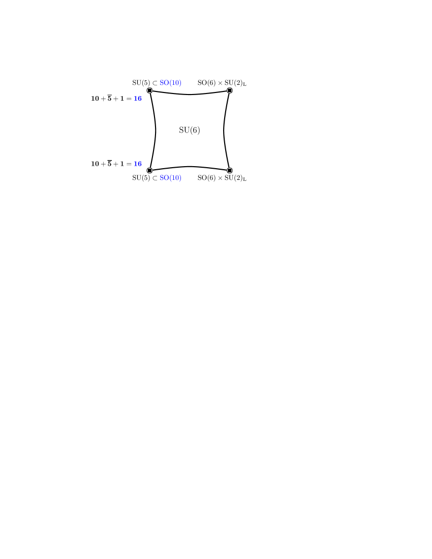
(a) $\mathrm{SO}(4)$ plane.

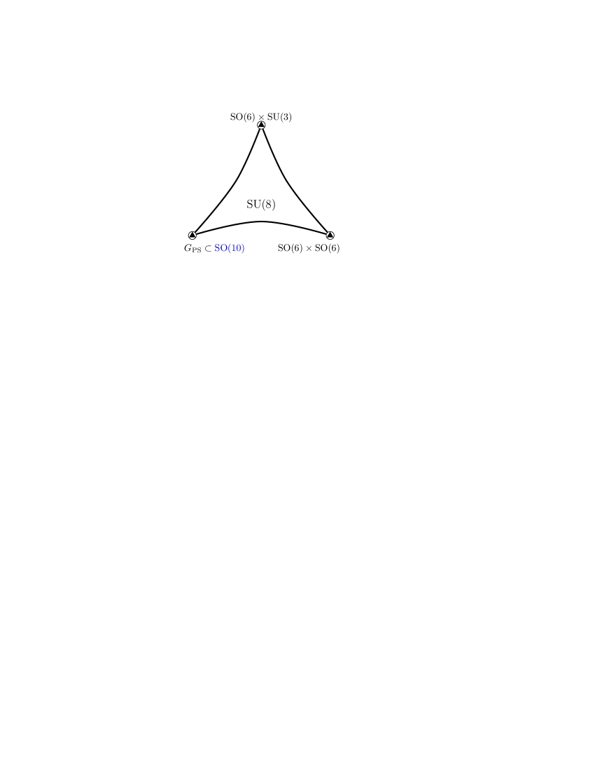
(b) $\mathrm{SU}(3)$ plane.

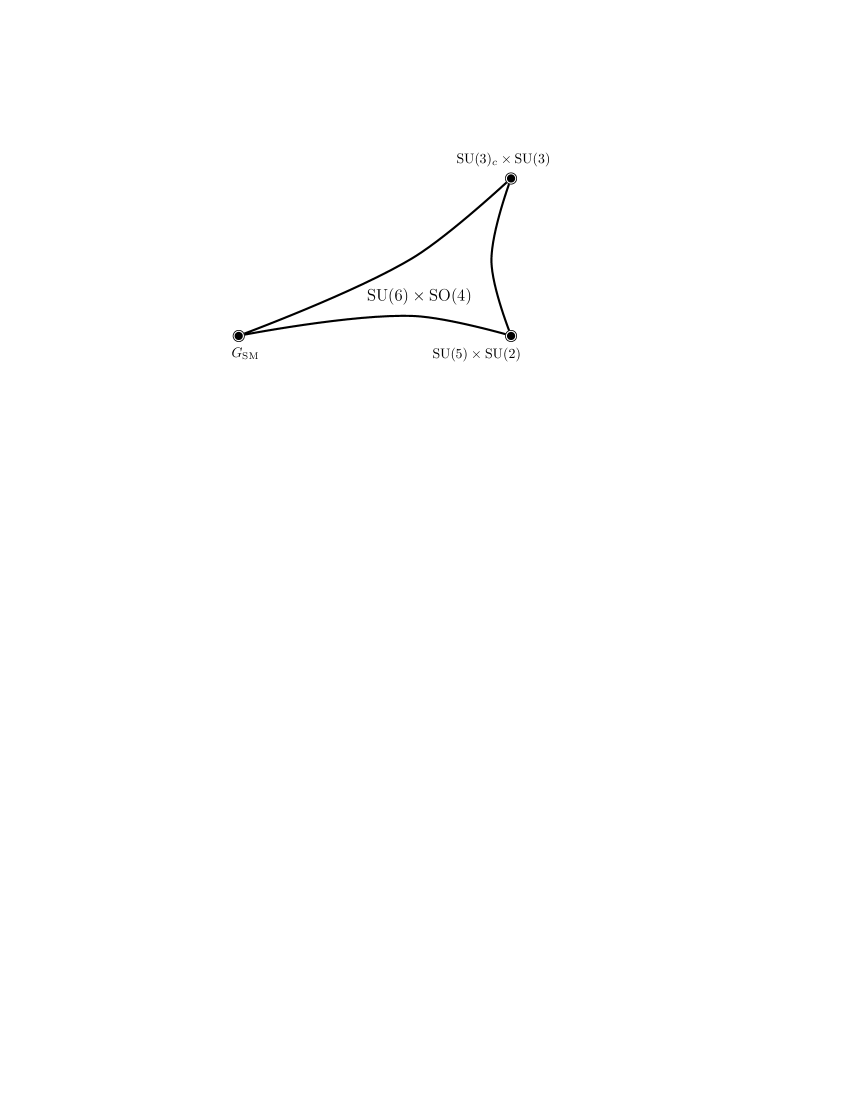
(c) $\mathrm{G}_{2}$ plane.

Figure 10: Orbifold GUT limits. In each case, a plane with a large compactification radius is displayed. Only subgroups of the first $\mathrm{E}_{8}$ are shown and $\mathrm{U}(1)$ factors are omitted.

One of the motivations for revisiting orbifold compactifications of the heterotic string is the phenomenological success of orbifold GUTs [14, 15, 16, 17, 18, 19]. In our model, the hypercharge is correctly normalized and the spectrum is that of the MSSM, which leads to gauge coupling unification at about $2\times 10^{16}$ GeV. It is therefore interesting to study orbifold GUT limits of the model, which correspond to anisotropic compactifications where some radii are significantly larger than the others. Such anisotropy may mitigate the discrepancy between the GUT and the string scales and can be consistent with perturbativity for one or two large radii of order $(2\times 10^{16}~{}{\rm GeV})^{-1}$ [59, 60]. In the energy range between the compactification scale and the string scale one obtains an effective higher-dimensional field theory.

In $\mathbbm{Z}_{6-\mathrm{II}}$ orbifolds, there are four independent radii: two are associated with the $\mathrm{G}_{2}$ and $\mathrm{SU}(3)$ planes, respectively, and the other two are associated with the two independent directions in the $\mathrm{SO}(4)$-plane. Any of these radii can in principle be large leading to a distinct GUT model.

The bulk gauge group and the amount of supersymmetry are found via a subset of the invariance conditions (2.53) with $N<6$. Consider a subspace ${\cal S}$ of the 6D compact space with large compactification radii. This subspace is left invariant under the action of some elements of the orbifold space group, i.e. a subset of twists and translations ${\cal G}$. The bulk gauge multiplet in ${\cal S}$ is part of the $N=4$ $\mathrm{E}_{8}\times\mathrm{E}_{8}$ gauge multiplet which is invariant under the action of ${\cal G}$, i.e. a subset of conditions (2.46) restricted to ${\cal G}$ [25].

In our model, the intermediate orbifold picture can have any dimensionality between 5 and 10. For example, the 6D orbifold GUT limits are (up to $\mathrm{U}(1)$ factors):

$$\mathrm{SO}(4)~{}\text{plane} : ~{}\text{bulk GUT}=\mathrm{SU}(6)~{},~{}N=2\;,$$

$$\mathrm{SU}(3)~{}\text{plane} : ~{}\text{bulk GUT}=\mathrm{SU}(8)~{},~{}N=2\;,$$

$$\mathrm{G}_{2}~{}\text{plane} : ~{}\text{bulk GUT}=\mathrm{SU}(6)\times\mathrm{SO}(4)~{},~{}N=4\;,$$

where the plane with a “large” compactification radius is indicated and $N$ denotes the amount of supersymmetry. In all of these cases, the bulk $\beta$–functions of the SM gauge couplings coincide. This is because either $G_{\mathrm{SM}}$ is contained in a simple gauge group or there is $N=4$ supersymmetry. It is remarkable that regardless of which radii are large, unification in the bulk occurs. This observation may indeed be relevant to the discrepancy between the GUT and the string scales. However, to check whether this is really the case, logarithmic corrections from localized fields, contributions from vector–like heavy fields and string thresholds have to be taken into account.

The 6D orbifold GUT limits of the model are displayed in Fig. 10. We note that the standard model gauge group is obtained as an intersection of the local gauge groups at the orbifold fixed points. For completeness, in Tab. D.13 we survey all possible orbifold GUT limits. For $D\geq 6$, we find that they are all consistent with gauge coupling unification in the bulk. The different geometries differ, however, in the values of the gauge couplings at the unification scale as well as the Yukawa couplings.

6 Supersymmetric vacuum configurations

In this section we discuss supersymmetric vacuum configurations of our model. In globally supersymmetric theories, these require vanishing of the $D$- and $F$–terms. We start with the discussion of the $D$–terms.

6.1 $\boldsymbol{D}$–flatness

In a supersymmetric gauge theory with an anomalous $\mathrm{U}(1)$, vanishing of the $D$–terms requires

$$D_{a} = \sum_{i}\phi_{i}^{*}T_{a}\phi_{i}=0\;,$$

$$D_{\mathrm{anom}} = \sum_{i}q_{\mathrm{anom}}^{(i)}\,|\phi_{i}|^{2}+\frac{g\,M_{\mathrm{P}}^{2}}{192\pi^{2}}~{}{\operatorname{tr}\mathsf{t}_{\mathrm{anom}}}=0\;,$$ (6.1)

where $T_{a}$ are generators of the gauge group and $\mathsf{t}_{\mathrm{anom}}$ is the generator of an anomalous $\mathrm{U}(1)$. In particular, to have a vanishing FI $D$–term, there must exist at least one field whose anomalous charge is opposite in sign to that of ${\operatorname{tr}\mathsf{t}_{\mathrm{anom}}}$.

In theories without an anomalous $\mathrm{U}(1)$, these conditions are satisfied if there exists a gauge invariant monomial $I(\phi_{i})$ [57]. The $D$–flat field configurations are found from

$$\left\langle{\partial I\over\partial\phi_{i}}\right\rangle~{}=~{}c\,\langle\phi_{i}^{*}\rangle\;,$$ (6.2)

where $c$ is a constant and $\langle x\rangle$ denotes the VEV of $x$. On solutions of this equation, gauge invariance of $I$ simply means $D_{a}=0$ [57]. If an anomalous $\mathrm{U}(1)$ is present, $D$–flatness requires the existence of $I(\phi_{i})$ which is gauge invariant with respect to all symmetries apart from $\mathrm{U}(1)_{\mathrm{anom}}$ and which carries a net anomalous charge whose sign is opposite to that of ${\operatorname{tr}\mathsf{t}_{\mathrm{anom}}}$ (see, e.g., [12, 61, 62]).

Therefore, searching for a $D$–flat configuration amounts to finding gauge invariant monomials with the above properties. Clearly, such monomials can be multiplied together while preserving the required properties. We are particularly interested in the $\mathrm{U}(1)^{N}$ gauge theory which is relevant when the non–Abelian singlets $s_{i}$ get VEVs. In this case, the gauge invariant monomial

$$(s_{1})^{n_{1}}\,(s_{2})^{n_{2}}\dots(s_{k})^{n_{k}}\;,\quad n_{i}\in\mathbbm{N}\;,$$ (6.3)

represents the $D$–flat direction

$$|s_{1}|/\sqrt{n_{1}}=|s_{2}|/\sqrt{n_{2}}~{}=~{}\dots~{}=~{}|s_{k}|/\sqrt{n_{k}}$$ (6.4)

in the field space. The overall scale of these VEVs is fixed by the FI $D$–term.

Starting with the anomalous $\mathrm{U}(1)$ $D$–term, an example of a gauge invariant monomial with a negative anomalous charge is given by

$$I_{1}~{}=~{}(s_{12})^{2}\,s_{39}\,s_{55}\,s_{56}\;.$$ (6.5)

Clearly, it is not unique (cf. Tab. LABEL:tab:GaugeInvariantMonomialsGen). In particular, it can be multiplied by a monomial with zero anomalous charge. We find that every $s_{i}$ that enters the mass matrices for the exotic states also enters a gauge invariant monomial (see Tab. LABEL:tab:GaugeInvariantMonomials). This shows that $s_{i}$ can be given large VEVs while having vanishing $D$–terms.

There is also another algorithm to check the $D$–flatness for the required singlet configuration. Mass terms for vector–like exotic matter $x_{i}$ are generated by

$$W~{}=~{}\sum_{ij}x_{i}\bar{x}_{j}\mathcal{M}_{ij}(s)$$ (6.6)

with

$$\mathcal{M}_{ij}(s)~{}=~{}\sum_{n}\sum_{k_{1},\dots,k_{n}}c_{ij}({k_{1}},\dots,{k_{n}})~{}s_{k_{1}}\dots s_{k_{n}}\;,$$ (6.7)

where $s_{k_{a}}$ are the singlets and $c_{ij}({k_{1}},\dots,{k_{n}})$ are some coefficients. Any monomial of fields in the superpotential is gauge invariant and represents a $D$–flat direction. Thus multiplying all of the monomials together, we again get a flat direction. However, we do not want to give VEVs to the exotic matter fields $x_{i}$ since this would break the standard model gauge group. So, one needs to replace those with some SM–singlets which have the same total $\mathrm{U}(1)$–charges:

$$\mathrm{U}(1)\text{-charges}\left(\prod_{M_{ij}\not=0}x_{i}\bar{x}_{j}\right)~{}=~{}\mathrm{U}(1)\text{-charges}\;\bigl{(}s_{l_{1}}\dots s_{l_{n}}\bigr{)}\;.$$ (6.8)

This is just one equation. In our case, there are many singlet monomials satisfying this equation and one of them is

$$s_{7}(s_{19})^{4}s_{26}s_{36}s_{39}(s_{40})^{5}(s_{48})^{18}s_{55}(s_{56})^{3}(s_{57})^{7}(s_{64})^{2}(s_{68})^{42}(s_{69})^{27}\;.$$ (6.9)

To cancel the FI term, one has to multiply it with the monomial $I_{1}$ which has a negative anomalous charge. This shows that one can give VEVs to all singlets involved in the decoupling of extra matter consistently with the $D$–flatness.

6.2 Some of the $\boldsymbol{F}$–flat directions

The requirement $F_{i}=0$ for a singlet $s_{i}$ is most easily satisfied if $s_{i}$ is an $F$–flat direction, i.e.,

$${\partial W\over\partial s_{i}}~{}=~{}0$$ (6.10)

for arbitrary values of $s_{i}$. (When $s_{i}$ is not a flat direction, $F_{i}=0$ is satisfied only at special values of $s_{i}$.) The existence of such flat directions usually requires that the VEVs of some other singlets appearing in the superpotential be zero.

Many exactly $F$–flat directions can be obtained from the selection rule (4.8c) for the superpotential couplings,

$$\sum R^{3}~{}=~{}-1\mod 2\;.$$ (6.11)

As seen from Tabs. LABEL:tab:LongTableNonSingletsSaturdayAfternoonModel and LABEL:tab:LongTableSingletsSaturdayAfternoonModel, all of the non–Abelian singlets in $U$, $T_{2}$, $T_{4}$ sectors have $R^{3}=0$. Thus they cannot couple among themselves consistently with the rule (6.11). Furthermore, they cannot couple to a single state in $T_{1,3}$ since the latter have $R^{3}=-1/2$ and at least two of such states are needed to have an allowed coupling. That means that the $F$–terms are proportional to a VEV of some state in $T_{1,3}$:

$$F_{i}~{}\sim~{}{\partial W\over\partial s_{i}}~{}\sim~{}\langle\text{singlet from}~{}T_{1,3}\rangle~{}=~{}0\;,$$ (6.12)

as long as all singlets in $T_{1,3}$ have zero VEVs. Thus one immediately gets 39 exactly $F$–flat directions associated with $s_{i}$ from the

$$U,~{}T_{2},~{}T_{4}$$ (6.13)

sectors. By this we mean that the 39 fields are allowed to attain non–zero VEVs simultaneously, without referring to the number of real variables parametrizing such VEVs.

One can also show that these directions are $D$–flat. In particular, each non–Abelian singlet from $U,T_{2},T_{4}$ enters a gauge invariant monomial which involves only $U,T_{2},T_{4}$ singlet states. Furthermore, it is possible to construct a monomial with a negative net anomalous charge. An example is (see also Tab. LABEL:tab:GaugeInvariantMonomialsFflat)

$$I~{}=~{}s_{34}\,s_{35}\,s_{40}\,s_{39}\,s_{67}\;.$$ (6.14)

That means one can give non–zero VEVs to the $U,T_{2},T_{4}$ singlets while preserving supersymmetry. Some of such states presumably correspond to the “blowing–up” modes of the orbifold which allow one to interpolate between a smooth Calabi–Yau manifold and an orbifold.

These flat directions allow us to decouple many exotic states but not all. One can perhaps increase the dimensionality of the $F$– and $D$–flat space by including non–Abelian flat directions or by other considerations. We also note that, for practical purposes, flatness is only required up to a certain order in superpotential couplings and one may exploit approximately flat directions.

In any case, flat directions are not necessary for the decoupling. As we discuss below, supersymmetric field configurations are in general more complicated and allow for the decoupling of the exotic states.

6.3 General supersymmetric field configurations

Given a set of 69 states $s_{i}$, supersymmetric field configurations are given by the sets of VEVs $\langle s_{i}\rangle$ which satisfy $F_{i}=D_{a}=0$. Naively, it appears that the number of constraints, that is 69 plus the number of the gauge group generators, is larger than the number of variables, 69. The system seems to be overconstrained. However, this is not the case. As well known, complexified gauge transformations allow us to eliminate the $D$–term constraints ([63],[64, Chapter VIII]), such that the number of variables equals the number of equations. In what follows, we demonstrate this for Abelian and non–Abelian cases.

6.3.1 Abelian case

Consider a supersymmetric $\mathrm{U}(1)^{N}$ gauge theory with $n$ charged fields $z_{i}$. The superpotential can be written as

$$W~{}=~{}\sum_{(a)}I^{(a)}(z_{1},\dots,z_{n})\;.$$ (6.15)

Here $I^{(a)}$ are gauge invariant monomials (some of which may be reducible, i.e. a product of lower order monomials),

$$I(z_{1},\dots,z_{n})~{}=~{}c\;z_{1}^{k_{1}}\dots z_{n}^{k_{n}}$$ (6.16)

with $c$ being a constant and

$$k_{1}\boldsymbol{Q_{1}}+\dots+k_{n}\boldsymbol{Q_{n}}~{}=~{}0\;,$$ (6.17)

where $\boldsymbol{Q_{i}}=(q^{1}_{i},\dots,q_{i}^{N})$ is an $N$–vector of $\mathrm{U}(1)$ charges of the fields $z_{i}$.

Supersymmetry is preserved in the vacuum if

$$F_{i}~{}=~{}0~{}~{},~{}~{}D_{a}~{}=~{}0\;,\quad i=1,\dots,n~{};~{}a=1,\dots,N\;.$$ (6.18)

Start with the $F$–terms. $F_{i}=0$ can be written as

$$F_{i}(z)~{}\equiv~{}{\partial W\over\partial z_{i}}~{}=~{}0$$ (6.19)

for all $i$. Since there are $n$ such equations and $n$ variables, there are solutions. In general, there are solutions with $z_{i}\not=0$ (for example, when $W$ is a non–trivial polynomial).

Consider a solution with $z_{i}\not=0$. Note that $F_{i}(z)$ is not gauge invariant, but transforms as $z_{i}^{-1}$. As a consequence, if $\{z_{k}^{0}\}$ is a solution to $F_{i}(z)=0$, then the transformation

$$z_{k}^{0}~{}\rightarrow~{}z_{k}^{\prime}~{}=~{}z_{k}^{0}~{}(\alpha_{1})^{q_{k}^{1}}(\alpha_{2})^{q_{k}^{2}}\cdots(\alpha_{N})^{q_{k}^{N}}\;,$$ (6.20)

leaves the $F$–terms vanishing,

$$F_{i}(z^{0})~{}\rightarrow~{}F_{i}(z^{\prime})~{}=~{}F_{i}(z^{0})~{}(\alpha_{1})^{-q_{i}^{1}}(\alpha_{2})^{-q_{i}^{2}}\cdots(\alpha_{N})^{-q_{i}^{N}}~{}=~{}0\;,$$ (6.21)

where $\alpha_{i}$ are arbitrary complex numbers and ${q_{i}^{a}}$ is the $a$-th $\mathrm{U}(1)$ charge of $z_{i}$. Therefore, given a solution $z_{i}^{0}$ to the $F$–term equations, it can be rescaled as above to give a family of solutions. In fact, it can be rescaled in such a way that all the $D$–terms vanish:

$$D_{a}(z^{\prime})~{}=~{}\sum_{i}q_{i}^{a}|z^{\prime}_{i}|^{2}~{}=~{}\sum_{i}q_{i}^{a}|z^{0}_{i}|^{2}|\alpha_{1}|^{2q_{i}^{1}}|\alpha_{2}|^{2q_{i}^{2}}\dots|\alpha_{N}|^{2q_{i}^{N}}~{}=~{}0$$ (6.22)

for $a=1,\dots,N$. The $N$ rescaling parameters $|\alpha_{i}|$ are found from the above $N$ equations. In terms of the rescaled variables $z^{\prime}_{i}$, these solutions are encoded in the gauge invariant monomials $z_{1}^{\prime\,k_{1}}\dots z_{n}^{\prime\,k_{n}}$ such that

$$|z_{1}^{\prime}|/\sqrt{k_{1}}~{}=~{}|z_{2}^{\prime}|/\sqrt{k_{2}}~{}=~{}\dots~{}=~{}|z_{3}^{\prime}|/\sqrt{k_{n}}$$ (6.23)

is a $D$–flat direction. This latter equation allows to find $\alpha_{i}$ most easily and also shows that sensible solutions to Eq. (6.22) exist, i.e. $|\alpha_{i}|^{2}>0$.

Let us now turn to the $D$–term of an anomalous $\mathrm{U}(1)$. The complexified gauge transformation which leaves $F_{i}=0$ intact is

$$z_{i}^{0}~{}\to~{}z^{\prime}_{i} = \alpha^{q_{\mathrm{anom}}^{(i)}}z_{i}^{0}\;,$$

$$D_{\mathrm{anom}}(z^{\prime}) = \sum_{i}q_{\mathrm{anom}}^{(i)}\,|z_{i}^{0}|^{2}|\alpha|^{2q_{\mathrm{anom}}^{(i)}}+\frac{g\,M_{\mathrm{P}}^{2}}{192\pi^{2}}~{}{\operatorname{tr}\mathsf{t}_{\mathrm{anom}}}\;.$$ (6.24)

As long as there is a field whose anomalous charge is opposite in sign to that of ${\operatorname{tr}\mathsf{t}_{\mathrm{anom}}}$, the $D$-term can be cancelled. Suppose ${\operatorname{tr}\mathsf{t}_{\mathrm{anom}}}<0$, then $D_{\mathrm{anom}}<0$ for $\alpha^{q_{\mathrm{anom}}^{(i)}}\rightarrow 0$ and $D_{\mathrm{anom}}>0$ for $\alpha^{q_{\mathrm{anom}}^{(i)}}\rightarrow\infty$. Therefore, there is a solution to $D_{\mathrm{anom}}=0$ for finite $\alpha^{q_{\mathrm{anom}}^{(i)}}$.

It is now clear that the $D$–term constraints can be satisfied by an appropriate choice of complexified gauge transformations. This means that the number of SUSY conditions $F_{i}=0$ equals the number of variables $z_{i}$, such that (non–trivial) solutions generally exist. Such solutions can be points (up to gauge transformations) or low dimensional manifolds in the field space.

6.3.2 Non–Abelian case

Let us now consider the case of a non–Abelian gauge theory following Ref. [64, Chapter VIII]. This situation arises in our construction when one assigns VEVs to the doublets of the hidden sector $\mathrm{SU}(2)$. As in the Abelian case, if $\{z_{k}^{0}\}$ is a solution to the $F$–term equations $F_{i}(z)=0$, then

$$z^{\prime}~{}=~{}\exp\left(\mathrm{i}\sum_{a}\lambda_{a}T_{a}\right)z^{0}$$ (6.25)

is also a solution, where $T_{a}$ are the group generators and $\lambda_{a}$ are complex parameters. This is because $F_{i}$ transforms as $z_{i}^{-1}$, i.e., $F(z^{\prime})=\exp(-\mathrm{i}\sum\lambda_{a}T_{a})F(z^{0})$.

The $D$–terms, $D_{a}(z)=\sum_{i}z_{i}^{\dagger}T_{a}z_{i}$, transform in the adjoint representation under this transformation. There is always a group element which transforms vector $D_{a}$ into $(x,0,..,0)$ corresponding to the direction of one of the Cartan generators $T_{\hat{a}}$, i.e. $D_{a}\rightarrow D_{\hat{a}}=\sum_{i}z_{i}^{\dagger}T_{\hat{a}}z_{i}$. Writing $(T_{\hat{a}})_{ij}=\mu_{i}\delta_{ij}$ with real $\mu_{i}$, the only non–vanishing $D$–term is

$$D_{\hat{a}}(z^{\prime})~{}=~{}\sum_{i}\mu_{i}|z^{\prime}_{i}|^{2}\;.$$ (6.26)

The complexified gauge transformation along this direction,

$$z^{\prime}_{i}~{}\to~{}z^{\eta}_{i}~{}=~{}\exp(\mu_{i}\eta)\,z^{\prime}_{i}\;,$$ (6.27)

with real $\eta$, leaves $F_{i}(z^{\eta})=0$ and transforms the $D$–term into

$$D_{\hat{a}}(z^{\eta})~{}=~{}\sum_{i}\mu_{i}e^{2\mu_{i}\eta}|z^{\prime}_{i}|^{2}\;.$$ (6.28)

In the non–degenerate case, $D_{\hat{a}}(z^{\eta})\to\pm\infty$ for $\eta\to\pm\infty$. Therefore, there is a solution to $D_{a}=0$ for finite $\eta$ and hence finite $z_{i}^{\eta}$.

6.3.3 Summary and applications

Employing complexified gauge symmetry, we have shown that the system of equations $F_{i}=D_{a}=0$ in globally supersymmetric models is not overconstraining. In particular, solutions to $F_{i}=0$ exist since the number of equations equals the number of complex variables and in general some of these solutions are non-trivial. Once a non–trivial solution to $F_{i}=0$ is found, it can be transformed using complexified gauge symmetry to satisfy $D_{a}=0$. This conclusion is based on the observation that the $F$–term equations constrain gauge invariant monomials, while such monomials are also associated with $D$–flat directions.

Consequently, supersymmetric field configurations in orbifold models form low dimensional manifolds or points (up to gauge transformations). In such configurations, SM singlets generally attain non–zero VEVs, typically not far below the string scale. As a result, when such VEVs play a role of the mass terms for vector–like exotic states, the decoupling of the latter can be made consistently with supersymmetry.

The above considerations apply to globally supersymmetric models at the perturbative level. In practice, we expect supergravity as well as non–perturbative effects to play a role in selecting vacua. However, it would be very difficult to quantify such effects at this stage. We note that, in existing literature, it is rather common to amend the global SUSY conditions $F_{i}=D_{a}=0$ by $\langle W\rangle=0$ (see e.g. [50]), which implies a vanishing cosmological constant in supergravity. Such a condition should however be imposed on the $total$ superpotential which includes, in particular, non–perturbative potentials for moduli. Thus, requiring $\langle W\rangle=0$ does not set any immediate constraint on the charged matter VEVs. At this stage, we include only the most important supergravity effect, that is gaugino condensation in the hidden sector, which we discuss in the next section.

7 Spontaneous supersymmetry breaking

7.1 Hidden sector gaugino condensation

As supersymmetry is broken in nature, realistic models should admit spontaneous supersymmetry breakdown. An attractive scheme for that is hidden sector gaugino condensation [65, 66, 67, 68]. In this case, a hierarchically small supersymmetry breaking scale, which is favoured by phenomenology, is explained by dimensional transmutation.

The basic idea is that one or more gauge groups in the hidden sector become strongly coupled at an intermediate scale. This leads to confinement and gaugino condensation. Under certain circumstances, that is if the dilaton is stabilized, gaugino condensation translates into supersymmetry breaking. In particular,

$$\langle\lambda\lambda\rangle^{1/3}~{}\sim~{}10^{13}\,\mathrm{GeV}\;,$$ (7.1)

leads to the gravitino mass in the TeV range, $m_{3/2}\sim\langle\lambda\lambda\rangle/M_{\mathrm{P}}^{2}$. The condensation scale $\Lambda\sim\langle\lambda\lambda\rangle^{1/3}$ is given by the Landau pole of the condensing gauge group,

$$\Lambda~{}=~{}M_{\mathrm{GUT}}\,\exp\left(-\frac{1}{2\beta}\frac{1}{g^{2}(M_{\mathrm{GUT}})}\right)\;.$$ (7.2)

For certain gauge groups and matter content, $\Lambda$ can be in the right range.

Gaugino condensation leads to supersymmetry breaking only if the dilaton is stabilized at a realistic value. Models with a single gaugino condensate and a classical Kähler potential suffer from the notorious dilaton run–away problem. That is, gaugino condensation creates a non–perturbative superpotential for the dilaton $W\sim\exp(-a\,S)\sim\langle\lambda\lambda\rangle$ (where $a=3/2\beta$) which leads to $S\rightarrow\infty$ at the minimum of the scalar potential. There are two common options to avoid this problem: employ multiple gaugino condensates or use non–perturbative corrections to the Kähler potential. The first option is not available in our model as the hidden sector $\mathrm{SU}(2)$ either does not condense or its condensation scale is too low, and we are left with a single $\mathrm{SU}(4)$. Thus, we use the second option. In this case, the classical Kähler potential for the dilaton is amended by non–perturbative corrections,

$$K~{}=~{}-\ln(S+\overline{S})+\Delta K_{\mathrm{np}}\;.$$ (7.3)

The functional form of $\Delta K_{\mathrm{np}}$ has been studied in the literature [69, 70, 71, 72, 73, 74]. For a favourable choice of the parameters, this correction allows one to stabilize the dilaton at a realistic value, $\operatorname{Re}S\simeq 2$, while breaking supersymmetry [71, 73, 74, 75, 76]. Supersymmetry is broken spontaneously by the dilaton $F$–term,

$$F_{S}~{}\sim~{}{\langle\lambda\lambda\rangle\over M_{\mathrm{P}}}~{},~{}F_{T}\sim 0~{},$$ (7.4)

where $T$ is the heterotic $T$–modulus. In what follows, we will estimate the gaugino condensation scale in our model without going into details of the dilaton stabilization mechanism.

The condensing gauge group in our case is $\mathrm{SU}(4)$. The condensation scale depends on the matter content. If all the singlets have zero VEVs, there are 5 $\boldsymbol{6}$–plets and 4 pairs of $\boldsymbol{4}+\overline{\boldsymbol{4}}$. The corresponding beta function is

$$\beta_{\mathrm{SU}(4)}~{}=~{}\frac{1}{16\pi^{2}}\left\{12-\#(\boldsymbol{6})-\#(\boldsymbol{4}+\overline{\boldsymbol{4}})\right\}\;,$$ (7.5)

where $\#(\boldsymbol{R})$ counts the number of representations $\boldsymbol{R}$. With the above matter content, $\mathrm{SU}(4)$ is asymptotically free but the condensation scale is too low. In a general field configuration, the $\boldsymbol{6}$–plets and the pairs $\boldsymbol{4}+\overline{\boldsymbol{4}}$ receive large masses (see Eqs. (D.32) and (D.38)) and are all decoupled. In this case, the beta function becomes

$$\beta_{\mathrm{SU}(4)}~{}=~{}\frac{3}{4\pi^{2}}\;.$$ (7.6)

The condensation scale is then $10^{10}-10^{11}$ GeV. There are many factors that can affect it. In particular, there are string threshold corrections [77, 78, 79, 80, 81] which lead to different gauge couplings in the visible and hidden $\mathrm{E}_{8}$. The corresponding gauge kinetic functions are given by [77, 80, 81]

$$f_{\mathrm{vis}/\mathrm{hid}}~{}=~{}S\pm\epsilon\,T\;,$$ (7.7)

where $\epsilon$ is a small parameter and, for simplicity, we have taken a large $T$ limit. The gauge couplings are found from

$$\operatorname{Re}f~{}=~{}g^{-2}\;.$$ (7.8)

In the visible sector, the apparent gauge coupling unification requires $g^{-2}_{\mathrm{GUT}}\simeq 2$, whereas the hidden sector gauge coupling is

$$g^{-2}_{\mathrm{hid}}(M_{\mathrm{GUT}})~{}=~{}\operatorname{Re}f_{\mathrm{hid}}~{}\simeq~{}2\,(1-\Delta)\;,$$ (7.9)

where $\Delta$ parametrizes string threshold corrections. The corresponding condensation scale is

$$\Lambda~{}\simeq~{}M_{\mathrm{GUT}}\,\exp\left[-\frac{1}{\beta}(1-\Delta)\right]\;.$$ (7.10)

For $\Delta$ between 0 and 0.3, the condensation scale ranges between $5\times 10^{10}$ and $10^{13}\,\mathrm{GeV}$ (cf. Fig. 11). Thus a TeV scale gravitino mass can in principle be obtained.

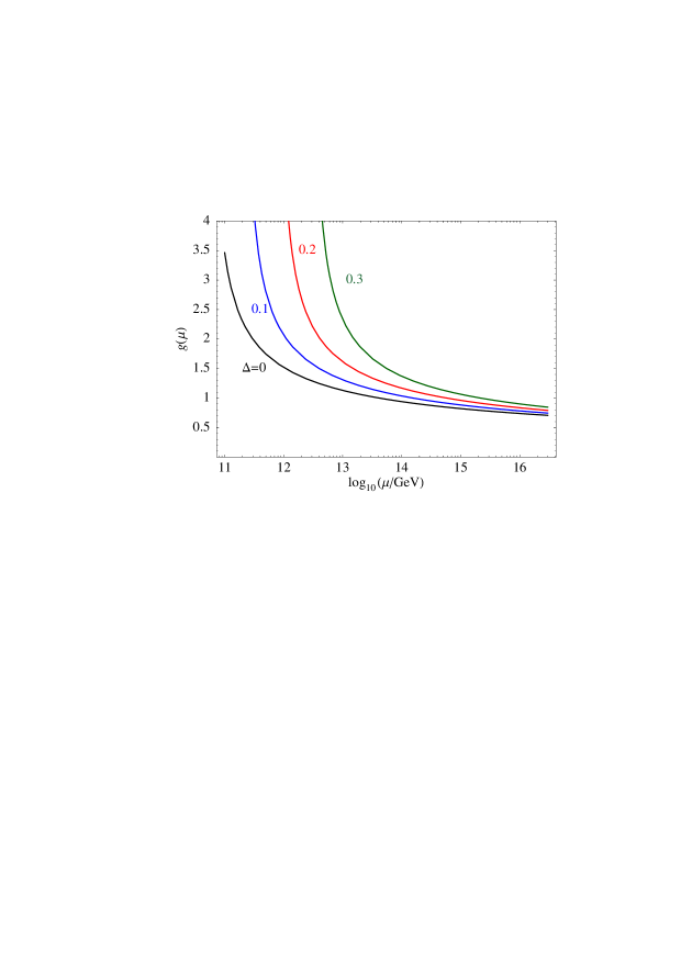
Figure 11: Scale dependence of the hidden sector $\mathrm{SU}(4)$ gauge coupling for different threshold corrections $\Delta$.

There are of course other factors that can affect the above estimate. For example, the SUSY breaking scale depends on coefficients entering a particular dilaton stabilization mechanism. Also the identification of the Landau pole with $\langle\lambda\lambda\rangle^{1/3}$ is not precise. The main point, however, is that the model contains the necessary ingredients for gaugino condensation and SUSY breaking in the phenomenologically interesting range.

7.2 Soft SUSY breaking terms

The Kähler stabilization mechanism leads to a specific pattern of the soft terms, the so called “dilaton dominated scenario” [82]. The resulting soft terms are universal and given by

$$\mathscr{L}_{\rm soft} = {1\over 2}(M\lambda^{a}\lambda^{a}+\text{h.c.})-m^{2}\phi^{*\alpha}\phi^{\alpha}-\left({1\over 6}A\;Y_{\alpha\beta\gamma}\phi^{\alpha}\phi^{\beta}\phi^{\gamma}+{\rm h.c.}\right)\;,$$ (7.11)

where $\lambda^{a}$ are the gauginos, $\phi^{\alpha}$ are the scalars and $Y_{\alpha\beta\gamma}$ are the Yukawa couplings. Dilaton dominated SUSY breaking implies the following relations among the soft breaking parameters (see e.g. [83]):

$$M~{}=~{}\pm\sqrt{3}m_{3/2}\;,\quad m~{}=~{}m_{3/2}\;,\quad A~{}=~{}-M\;.$$ (7.12)

This is a restricted version of mSUGRA with the only independent parameter being the gravitino mass $m_{3/2}$. Here we do not discuss the $\mu$ and $B\mu$ terms which depend on further details of the model.

The dilaton dominated scenario has a number of phenomenologically attractive features. In particular, due to flavour universality in the soft breaking sector, it avoids the SUSY FCNC problem. Also, most of the physical CP phases, e.g. $\arg(A^{*}M)$, vanish which ameliorates the SUSY CP problem. Other phenomenological aspects have been discussed in Ref. [84].

The above considerations are based on the assumption that the dilaton is stabilized via non–perturbative corrections to the Kähler potential. Dilaton and other moduli stabilization is a difficult issue and there may exist other possibilities which could lead to other patterns of the soft terms.

8 $\boldsymbol{B\!-\!L}$ symmetry and phenomenology

Realistic string vacua must satisfy a number of phenomenological constraints, in addition to those imposed by the spectrum and the gauge group of the MSSM. In particular, the proton should be sufficiently stable as well as flavour structures should be realistic. This constrains vacuum configurations for the SM singlets. In generic vacua, there are baryon number violating operators already at the renormalizable level, so in order to avoid rapid proton decay one must be able to tune the VEVs and suppress such operators. This appears rather artificial and one may ask whether there is a deeper reason behind it.

In this section, we explore vacua preserving the $B\!-\!L$ symmetry at the high energy (GUT) scale, which appear phenomenology attractive. In this case, the renormalizable $R$–parity violating couplings

$$W_{\cancel{R}}~{}=~{}\mu_{i}\,\ell_{i}\,\phi_{u}+\lambda_{ijk}\ell_{i}\,\ell_{j}\,\overline{e}_{k}+\lambda^{\prime}_{ijk}\ell_{i}\,q_{j}\,\overline{d}_{k}+\lambda^{\prime\prime}_{ijk}\overline{u}_{i}\,\overline{d}_{j}\,\overline{d}_{k}$$ (8.1)

are prohibited, leading to suppression of proton decay. The $B\!-\!L$ symmetry fits naturally into the concept of local GUTs: it is related to the $\mathrm{SO}(10)$ $B\!-\!L$ generator, although there are differences. Finally, $B\!-\!L$ can be broken at an intermediate scale which might induce small $R$–parity violating couplings and could be related to the smallness of the neutrino masses.

Having suppressed $B\!-\!L$ violation, we further study whether the required singlet VEV configurations allow for the decoupling of the exotic matter, realistic flavour structures and a small $\mu$–term.

In this section, we study a particular singlet VEV configuration for which we are able to prove the $D$–flatness, but not the $F$–flatness. Since the phenomenological analysis is intractable for the general case, we hope that the considerations below will provide some guidance to the further search for realistic vacua.

8.1 Vacuum configurations with unbroken $\boldsymbol{B\!-\!L}$

The first step is to obtain singlet VEV configurations which preserve

$$G_{\mathrm{SM}}\times\mathrm{U}(1)_{B\!-\!L}\times[\mathrm{SU}(4)]\;.$$

Here we keep the hidden sector $\mathrm{SU}(4)$ unbroken which is needed for gaugino condensation.

Let us now identify a $B\!-\!L$ generator. An obvious option would be to use the $B\!-\!L$ of SO(10). This however leads to anomalous $B\!-\!L$ symmetry, $\mathsf{t}_{B\!-\!L}^{\mathrm{SO}(10)}\cdot\mathsf{t}_{\mathrm{anom}}\neq 0$. It is possible to modify this generator such that the resulting $B\!-\!L$ is non–anomalous and the $B\!-\!L$ charges for the members of the $\boldsymbol{16}$–plets are the standard ones. Requiring further that the hidden sector $\mathrm{SU}(2)$ doublets $h_{i}$ be neutral under $\mathrm{U}(1)_{B\!-\!L}$, fixes

$$\mathsf{t}_{B\!-\!L}~{}=~{}\left(0,1,1,0,0,-\frac{2}{3},-\frac{2}{3},-\frac{2}{3}\right)\,\left(\frac{1}{2},\frac{1}{2},\frac{1}{2},-\frac{1}{2},0,0,0,0\right)\;.$$ (8.2)

The $B\!-\!L$ charges of matter fields are shown in Tabs. 8.1, D.3-D.3. The $q_{i}$ and $\overline{u}_{i}$ states have the standard charges, while only four out of seven $\overline{d}_{i}$ have the right charge ($-1/3$) to be identified with the down type anti–quarks. The $\overline{d}_{i}$ states with exotic $B\!-\!L$ charges as well as one linear combination of the $\overline{d}_{i}$’s with charge $-1/3$ pair up with four $d_{i}$’s and decouple from the low energy spectrum. Similar considerations apply to the lepton sector. The lepton doublets carry charge $-1$, while the Higgs doublets are neutral. One pair of $\ell_{i}$ and $\overline{\ell}_{i}$ with $q_{B\!-\!L}=0$ must remain in the massless spectrum and is identified with the physical Higgs bosons.

Among the 69 SM singlets $s_{i}$, 30 are neutral under $B\!-\!L$ , 21 have charge $+1$ and 18 have charge $-1$ (cf. Tab. D.3). This excess of positively charged $s_{i}$ leads to a net number of three ‘right–handed’ neutrinos.

field $B\!-\!L$ charges $q_{i}$ $\left\{\frac{1}{3},\frac{1}{3},\frac{1}{3}\right\}$ $\bar{u}_{i}$ $\left\{-\frac{1}{3},-\frac{1}{3},-\frac{1}{3}\right\}$ $\bar{d}_{i}$ $\left\{-\frac{1}{3},-\frac{1}{3},\frac{2}{3},-\frac{1}{3},-\frac{1}{3},\frac{2}{3},\frac{2}{3}\right\}$ $d_{i}$ $\left\{-\frac{2}{3},-\frac{2}{3},-\frac{2}{3},\frac{1}{3}\right\}$ $\ell_{i}$ $\{0,-1,-1,0,0,0,-1,-1\}$ $\bar{\ell}_{i}$ $\{0,0,0,1,0\}$ $\bar{e}_{i}$ $\{1,1,1\}$

Table 8.1: $B\!-\!L$ charges of the relevant matter fields.

Let us now consider configurations in which only states neutral under $G_{\mathrm{SM}}\times\mathrm{U}(1)_{B\!-\!L}\times[\mathrm{SU}(4)]$ are allowed to develop VEVs. Such states include $s_{i}$ with zero $q_{B\!-\!L}$ and the $\mathrm{SU}(2)^{\prime}$ doublets $h_{i}$. For our purposes, it suffices to restrict ourselves to a certain subset of these fields. In particular, we assume that

$$\langle s_{2},s_{5},s_{7},s_{9},s_{20},s_{23},s_{34},s_{41},s_{48},s_{58},s_{59},s_{62},s_{65},s_{66},\;$$

$$h_{1},h_{3},h_{6},h_{8},h_{9},h_{10},h_{11},h_{12},h_{13}\rangle = 0\;,$$ (8.3)

while

$$\{\widetilde{s}_{i}\} = \left\{s_{1},s_{3},s_{12},s_{14},s_{16},s_{18},s_{19},s_{22},s_{24},s_{39},s_{40},s_{53},s_{54},s_{57},s_{60},s_{61},\right.$$ (8.4)

$$\left.{}{\hphantom{\left\{\right.}}h_{2},h_{4},h_{5},h_{7},h_{14}\right\}$$

develop non–zero VEVs. We find that such a configuration is $D$–flat since every field from $\{\widetilde{s}_{i}\}$ enters a gauge invariant monomial consisting exclusively of $\{\widetilde{s}_{i}\}$ states (Tab. LABEL:tab:GaugeInvariantMonomials2). Also, it is possible to construct a monomial out of these states which has a negative net anomalous charge (Tab. LABEL:tab:GaugeInvariantMonomialsNC). The set $\{\widetilde{s}_{i}\}$ does not represent an $F$-flat direction. To preserve supersymmetry, we assume that there exist non–trivial field configurations in $\{\widetilde{s}_{i}\}$ with vanishing $F$–terms. Then, as described in Sec. 6, complexified gauge transformations allow us to satisfy $D_{a}=0$ at the same time. The set $\{\widetilde{s}_{i}\}$ breaks all extra $\mathrm{U}(1)$’s but $\mathrm{U}(1)_{B\!-\!L}$.

8.2 Decoupling the exotic states

The first question is whether it is possible to decouple all of the exotic states by giving VEVs to the set $\{\widetilde{s}_{i}\}$ only. To answer this question, we recalculate the mass matrices for the exotic matter. The relevant superpotential couplings are of the form

$$W~{}=~{}x_{i}\,\bar{x}_{j}\,\mathcal{M}_{x}^{ij}(\widetilde{s})\quad\text{with}\quad\mathcal{M}_{x}^{ij}(\widetilde{s})~{}=~{}\sum\widetilde{s}_{i_{1}}\cdots\widetilde{s}_{i_{n}}\;,$$ (8.5)

and $x_{i},\bar{x}_{j}$ being the vector–like pairs. Including the couplings up to order 10, the resulting mass matrices are

$$\mathcal{M}_{d}^{ij}(\widetilde{s}) = \left(\begin{array}[]{ccccccc}0&0&\widetilde{s}^{6}&0&0&\widetilde{s}^{6}&\widetilde{s}^{6}\\ 0&0&\widetilde{s}^{6}&0&0&\widetilde{s}^{7}&\widetilde{s}^{7}\\ 0&0&\widetilde{s}^{6}&0&0&\widetilde{s}^{7}&\widetilde{s}^{7}\\ \widetilde{s}^{8}&0&0&\widetilde{s}^{6}&\widetilde{s}^{6}&0&0\end{array}\right)\;,$$ (8.10)

$$\mathcal{M}_{\ell}^{ij}(\widetilde{s}) = \left(\begin{array}[]{cccccccc}\widetilde{s}^{3}&0&0&0&0&\widetilde{s}^{8}&0&0\\ \widetilde{s}&0&0&0&0&\widetilde{s}^{6}&0&0\\ \widetilde{s}&0&0&0&0&\widetilde{s}^{6}&0&0\\ 0&\widetilde{s}^{8}&\widetilde{s}^{8}&0&0&0&\widetilde{s}^{6}&\widetilde{s}^{6}\\ \widetilde{s}&0&0&\widetilde{s}^{6}&\widetilde{s}^{6}&0&0&0\end{array}\right)\;.$$ (8.16)

Here the columns in $\mathcal{M}_{d}^{ij}$ correspond to $\bar{d}_{j}$ and the rows to $d_{i}$; in $\mathcal{M}_{\ell}^{ij}$, the columns correspond to $\ell_{j}$ and the rows to $\bar{\ell}_{i}$. $\mathcal{M}_{m}^{ij}(\widetilde{s})$, $\mathcal{M}_{s}^{ij}(\widetilde{s})$, $\mathcal{M}_{f}^{ij}(\widetilde{s})$, and $\mathcal{M}_{w}^{ij}(\widetilde{s})$ are given by Eqs. (D.47)–(D.76) in App. D.4. As before, an entry $\widetilde{s}^{N}$ implies that there is an allowed coupling involving $N$ states $\widetilde{s}_{i}$. For instance, the $d_{1},\bar{d}_{3}$ mass term includes

$$W_{d_{1}\bar{d}_{3}}~{}=~{}d_{1}\bar{d}_{3}(s_{16}\,s_{40}\,h_{4}\,h_{14}\,h_{5}\,h_{14}+\cdots)\;.$$ (8.17)

Although the form of the mass matrices is quite restricted, all of them have the maximal rank, apart from the $\bar{\ell}_{i},\ell_{j}$ matrix whose rank is 4. This means that all of the exotic states are decoupled and one Higgs pair $\bar{\ell},\ell$ is massless, as required.

Clearly, some of the zeros of the mass matrices are dictated by the $B\!-\!L$ symmetry (see Tabs. 8.1, D.3, D.3). The massless down type anti–quarks are 3 linear combinations of the 4 $\bar{d}_{i}$ states with $q_{B\!-\!L}=-1/3$, namely $\bar{d}_{1}$, $\bar{d}_{2}$, $\bar{d}_{4}$ and $\bar{d}_{5}$. The remaining linear combination couples to $d_{4}$ and becomes heavy. Likewise, the physical lepton doublets are the 3 linear combinations of $\ell_{2}$, $\ell_{3}$, $\ell_{7}$ and $\ell_{8}$ which do not couple to $\bar{\ell}_{4}$. Interestingly, this type of structure has recently been explored in the context of orbifold GUTs [24]. It was shown that a mixing between chiral and vector–like states can lead to realistic flavour patterns.

Not all texture zeros can be understood from the $B\!-\!L$ symmetry. For instance, $B\!-\!L$ does not forbid the $\bar{\ell}_{1},\ell_{j>1}$ couplings such that additional input is needed. As we shall see, these zeros are crucial for identification of the Higgs doublets.

8.3 Higgs doublets and flavour structure

In our model, the only renormalizable $B\!-\!L$ conserving Yukawa coupling which involves SM matter is

$$W=g~{}q_{1}\,\bar{u}_{1}\,\bar{\ell}_{1}\;.$$ (8.18)

This is a superpotential of the type

$$U_{1}\,U_{2}\,U_{3}$$ (8.19)

with the untwisted superfields $U_{i}$ formed out of the compactified components of the $\mathrm{E}_{8}$ gauge multiplets in 10D. For example, for the scalar components we have $\tilde{U}_{1}\propto A_{4}+\mathrm{i}A_{5}$, etc., where $A_{i}$ are the gauge field components in the compact directions. This can be understood by recalling that the gauge supermultiplet in 10D decomposes into 1 vector and 3 chiral $N=1$ multiplets in 4D. The above superpotential results from the kinetic term of the gauge supermultiplet in 10D with the corresponding Yukawa coupling being the gauge coupling at the string scale.

As long as $\bar{\ell}_{1}$ has a significant component in the physical up–type Higgs doublet, the superpotential (8.18) naturally leads to a heavy top quark. The top Yukawa coupling is then of the order of the gauge coupling at the string scale,

$$Y_{t}~{}\sim~{}g\;.$$ (8.20)

This remarkable top Yukawa–gauge unification (Fig. 12) stems from the fact that the top quark is a gaugino in 10D. The other quark Yukawa couplings vanish at the renormalizable level. We note that a large top Yukawa coupling has also been obtained in earlier analyses of the fermion masses [85] - [87], [22].

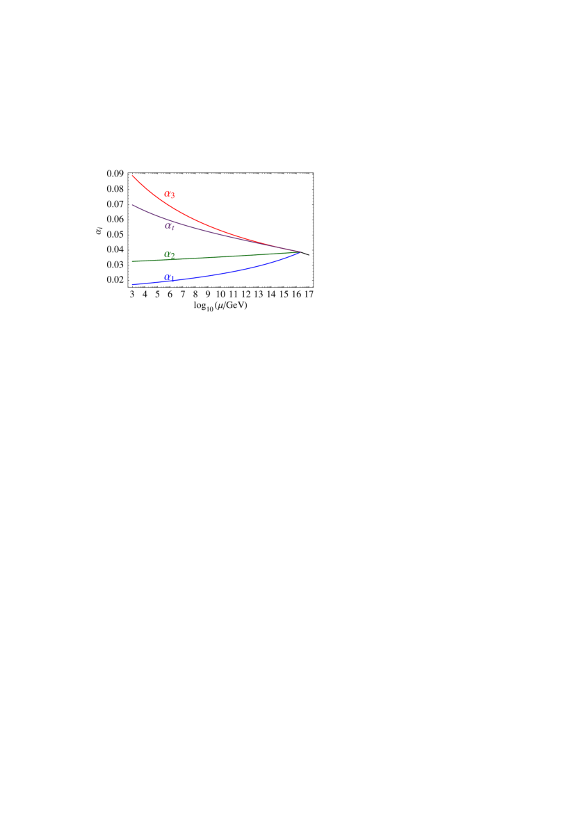
Figure 12: An idealized picture of gauge–top Yukawa unification. Here $\alpha_{i}=g_{i}^{2}/(4\pi)$, $\alpha_{t}=Y_{t}^{2}/(4\pi)$ and we have assumed that $Y_{t}=g_{i}$ at the GUT scale.

This attractive mechanism is at work when $\bar{\ell}_{1}\simeq\phi_{u}$. Inspection of the $\ell_{i}\bar{\ell}_{j}$ mass matrix (8.16) shows that the first 3 rows are linearly dependent and the $\bar{\ell}_{1}\,\ell_{1}$ coupling appears only at order 5 while the $\bar{\ell}_{i}\,\ell_{1}$ couplings with $i=2,3$ occur already at order 3. Thus, if the relevant $\tilde{s}_{i}$ VEVs are below the string scale, one expects at least mild suppression of the $(1,1)$ entry. Then, the massless up-type Higgs is dominated by $\bar{\ell}_{1}$,

$$\phi_{u}~{}\simeq~{}\bar{\ell}_{1}+\sum\limits_{i=2,3}\varepsilon_{i}\bar{\ell}_{i}\;,\quad|\varepsilon_{i}|\ll 1\;,$$ (8.21)

whereas the down-type Higgs is a linear combination of $\ell_{4}$ and $\ell_{5}$,

$$\phi_{d}~{}=~{}\ell_{4}\,a+\ell_{5}\,b\;,\quad$$ (8.22)

with $|a|,\,|b|$ of order one. Our choice of the vacuum configuration $\widetilde{s}_{i}$ (Eq. (8.4)) was in part motivated by these considerations.

At this stage, the Higgs doublets $\phi_{u,d}$ are massless. In contrast to the conventional 4D GUTs, no finetuning is required to keep the doublets light while decoupling the color triplets. If the $B\!-\!L$ symmetry gets broken at an intermediate scale, a small $\mu$-term will be generated.

Having identified the Higgs doublets and the top quark, we turn to the discussion of the remaining Yukawa couplings. The relevant superpotential is

$$W_{\mathrm{Yukawa}}~{}=~{}Y_{u}^{ij}(\widetilde{s})\,\phi_{u}\,q_{i}\,\bar{u}_{j}+Y_{d}^{ia}(\widetilde{s})\,\phi_{d}\,q_{i}\,\bar{d}_{a}+Y_{e}^{ib}(\widetilde{s})\,\phi_{d}\,\bar{e}_{i}\,\ell_{b}\;,$$ (8.23)

where $a\in\{1,2,4,5\}$ and $b\in\{2,3,7,8\}$. The Yukawa matrices at order 10 are

$$Y_{u}^{ij}(\widetilde{s}) = \left(\begin{array}[]{ccc}g&\widetilde{s}^{6}&\widetilde{s}^{4}\\ \widetilde{s}^{3}&0&\widetilde{s}^{7}\\ \widetilde{s}^{7}&\widetilde{s}^{7}&0\end{array}\right)\;,$$ (8.27)

$$Y_{d}^{ia}(\widetilde{s}) = \left(\begin{array}[]{cccc}0&\widetilde{s}^{6}&\widetilde{s}^{2}&\widetilde{s}^{2}\\ \widetilde{s}^{5}&0&\widetilde{s}^{5}&\widetilde{s}^{5}\\ 0&\widetilde{s}^{5}&\widetilde{s}&\widetilde{s}\end{array}\right)\;,$$ (8.31)

$$Y_{e}^{ib}(\widetilde{s}) = \left(\begin{array}[]{cccc}0&\widetilde{s}^{6}&0&0\\ \widetilde{s}^{5}&0&0&0\\ 0&\widetilde{s}^{5}&0&0\end{array}\right)\;.$$ (8.35)

The low-energy $3\times 3$ $Y_{d}$ and $Y_{e}$ Yukawa matrices are obtained by integrating out one linear combination of $\bar{d}_{a}$ ($a=1,2,4,5$) which pairs up with $d_{4}$ and one linear combination of $\ell_{b}$ ($b=2,3,7,8$) which pairs up with $\bar{\ell}_{4}$. Their precise form depends on various coefficients, so let us only discuss their main features.

The quark Yukawa matrices have the full rank such that, in general, there are no massless eigenstates. The lepton Yukawa matrix has rank 2 implying that the electron is massless to order 8 in the superpotential. Also, there appears one massless pair of $f$–plets in the hidden sector, which somewhat lowers the gaugino condensation scale.

Assuming that the relevant $\widetilde{s}_{i}$ have VEVs below the string scale, the Yukawa couplings are hierarchical and resemble the Froggatt–Nielsen structure [40]. However, the hierarchy appears due to the string selection rules rather than the $\mathrm{U}(1)$ charge assignment only as in the original Froggatt–Nielsen mechanism.

It is remarkable that the up–type quarks tend to be heavier than the down–type quarks, which in turn are heavier than the leptons. We also note that the Yukawa matrices generally contain non–trivial CP phases due to complex $\tilde{s}_{i}$ VEVs.

8.4 Proton stability and $\boldsymbol{B\!-\!L}$ breakdown

The $B\!-\!L$ symmetry enforces absence of renormalizable operators leading to proton decay. However, non–renormalizable $B\!-\!L$ conserving operators such as

$$W~{}=~{}\kappa_{ijkl}^{(1)}~{}q_{i}\,q_{j}\,q_{k}\,\ell_{l}+\kappa_{ijkl}^{(2)}~{}\bar{u}_{i}\,\bar{u}_{j}\,\bar{d}_{k}\,\bar{e}_{l}$$ (8.36)

also induce proton decay. The resulting constraint on $\kappa_{ijkl}^{(1)}$ and $\kappa_{ijkl}^{(2)}$ involving the first two generations is very tight [88, 89],

$$\kappa_{ijkl}^{(1,2)}~{}\lesssim~{}\frac{10^{-8}}{M_{\mathrm{P}}}\;.$$ (8.37)

The operators (8.36) are induced both directly and by integrating out the vector–like matter. For example, integrating out a heavy pair $d_{2}\bar{d}_{6}$ from the superpotential $W=q_{2}q_{2}d_{2}+q_{3}\ell_{3}\bar{d}_{6}$ yields $W\sim q_{2}q_{2}q_{3}\ell_{3}$. These operators can be suppressed either by tuning the $\tilde{s}_{i}$ VEVs or by an additional, perhaps discrete, symmetry [90, 91]. This issue will be discussed elsewhere.

Breaking $B\!-\!L$ is a difficult issue. It has to occur at an energy scale $M_{B\!-\!L}$ well below $M_{\mathrm{string}}$. In the following, we assume that the scale $M_{B\!-\!L}$ is generated dynamically, without breaking SUSY.

$B\!-\!L$ breaking VEVs fill in the zeros of the mass matrices, in particular, (8.16). This generates the $\mu$–term, $W=\mu~{}\phi_{u}\phi_{d}$. Assuming that apart from $\tilde{s}_{i}$, only states charged under $B\!-\!L$ get non–zero VEVs, its magnitude is ($n\geq 1$)

$$\mu~{}\sim~{}\frac{M_{B\!-\!L}^{n+1}}{M_{\mathrm{string}}^{n}}\;.$$ (8.38)

For an intermediate scale $M_{B\!-\!L}$, this can give a phenomenologically viable $\mu$–term.

$B\!-\!L$ breakdown generates masses for the right–handed neutrinos. Our construction has the necessary ingredients for the seesaw, i.e., neutrino Yukawa couplings and large Majorana neutrino masses. A detailed analysis of this issue will be presented elsewhere.

Finally, small $R$–parity violating couplings are generated. Their magnitude is given by $(M_{B\!-\!L}/M_{\mathrm{string}})^{m}$ with $m$ depending on the type of the coupling. For $m\geq 2$, an intermediate scale $M_{B\!-\!L}$ suppresses proton decay sufficiently [92].

To conclude, in this section we have studied a vacuum configuration with conserved $B\!-\!L$ at the string scale. This suppresses renormalizable $R$–parity violating couplings as well as the $\mu$–term. Furthermore, flavour structures à la Froggatt–Nielsen arise as a consequence of the string selection rules.

9 Outlook

Guided by the idea of local grand unification we have constructed an orbifold compactification of the heterotic string which leads to the supersymmetric standard model gauge group and particle content. The model has large vacuum degeneracy. For certain vacua with unbroken $B\!-\!L$ symmetry, the resulting phenomenology is particularly attractive. In this case, one pair of Higgs doublets is massless automatically, with the subsequently generated $\mu$–term being due to $B\!-\!L$ breaking. The top quark Yukawa coupling is of the order of the gauge coupling and the arising pattern of Yukawa couplings is reminiscent of the Froggatt-Nielsen textures.

These results can be the first steps towards a fully realistic theory. They immediately lead, however, to further questions which concern detailed properties of SUSY vacua, $B\!-\!L$ breakdown, incorporation of the seesaw mechanism, identification of $R$–parity and proton decay. Furthermore, effects of string threshold corrections and other contributions on gauge coupling unification have to be studied. Eventually, one would like to determine quantitatively the Yukawa couplings for specific supersymmetric vacua.

On the conceptual side, a deeper understanding of the decoupling of exotic states is particularly desirable. Orbifolds often represent special points in the moduli space of more general Calabi–Yau compactifications. Non–zero vacuum expectation values of specific standard model singlets correspond to other points in the moduli space where the orbifold singularities have been blown up. Since these vacuum expectation values also generate mass terms, at least some of the unwanted exotic states should be absent in compactifications on smooth manifolds. The orbifold limit of Calabi-Yau compactifications is well understood for the standard embedding [93] but remains to be studied in detail for non–standard embeddings which are relevant to the models presented in this paper.

Finally, it is important to search for other models in the framework of the $\mathrm{E}_{8}\times\mathrm{E}_{8}$ and the $\mathrm{SO}(32)$ heterotic string with localized $\boldsymbol{16}$–plets of $\mathrm{SO}(10)$ [94, 95]. It would also be very interesting to understand the connection between orbifold compactifications and compactifications on Calabi–Yau manifolds endowed with vector bundles [37, 36, 96, 97, 98], which have many phenomenologically appealing features.

Acknowledgments

We would like to thank R. Blumenhagen, M. Cvetic̆, A. Hebecker, T. Kobayashi, W. Lerche, M. Lindner, J. Louis, F. Plöger, S. Raby, S. Ramos-Sánchez, S. Stieberger, S. Theisen, P. K. S. Vaudrevange and in particular H. P. Nilles for valuable discussions. We are indebted to P. K. S. Vaudrevange for pointing out an error in the string selection rules presented in an earlier version of this paper.

This work was partially supported by the EU 6th Framework Program MRTN-CT-2004-503369 “Quest for Unification” and MRTN-CT-2004-005104 “ForcesUniverse” as well as the virtual institute VIPAC of the Helmholtz society.

Appendix A Sample calculations

In this appendix, we present details of the spectrum calculation for our model. These calculations are straightforward but tedious. For practical purposes, it is convenient to automatize them by means of a computer algebra system.

A.1 Gauge group

The 4D gauge group is obtained by subjecting the $\mathrm{E}_{8}$ roots $p$ ($p^{2}=2$) to the projection conditions

$$p\cdot V_{6} \in \mathbbm{Z}\;,$$ (A.1a)

$$p\cdot W_{2} \in \mathbbm{Z}\;,$$ (A.1b)

$$p\cdot W_{3} \in \mathbbm{Z}\;.$$ (A.1c)

Consider condition (A.1a). The roots of the first $\mathrm{E}_{8}$ surviving the twist are

$$p~{}\in~{}\left\{\pm(1,1,0^{6}),\pm(1,-1,0^{6}),\pm(0^{3},\underline{1,1,0,0,0}),(0^{3},\underline{1,-1,0,0,0})\right\}\;,$$ (A.2)

where the underline denotes permutations and the superscripts indicate repeated entries. The simple roots are by definition the smallest linearly independent positive roots (cf. [99]). For a suitable choice of positivity, they read

$$\{p_{\mathrm{sr}}\}~{}=~{}\left\{(1,1,0^{6}),(1,-1,0^{6}),\right.$$ (A.3)

$$\phantom{\left\{\right.}\left.(0^{3},1,-1,0^{3}),(0^{4},1,-1,0^{2}),(0^{5},1,-1,0),(0^{6},1,-1),(0^{6},1,1)\right\}\;.$$

Calculating the Cartan matrix $A_{ij}=p_{\mathrm{sr}}^{i}\cdot p_{\mathrm{sr}}^{j}$, one finds that the simple roots in the first line correspond to the raising operators of two $\mathrm{SU}(2)$ factors whereas those in the second line correspond to $\mathrm{SO}(10)$. Thus, the gauge group after twisting is $\mathrm{SO}(10)\times\mathrm{SU}(2)^{2}$, which also corresponds to the local gauge symmetry at the origin (cf. Tab. LABEL:tab:LocalGUTs).

The Wilson line projections (A.1b) and (A.1c) lead to the simple roots

$$\left\{(0^{5},1,-1,0),(0^{6},1,-1),(0^{3},1,-1,0^{3})\right\}\;,$$ (A.4)

which correspond to the gauge groups $\mathrm{SU}(3)$ and $\mathrm{SU}(2)$ in 4D. All $\mathrm{E}_{8}$ Cartan generators survive the projection. They give rise to the Cartan generators of $\mathrm{SU}(3)$ and $\mathrm{SU}(2)$ and to five $\mathrm{U}(1)$ generators. The latter can be represented by vectors perpendicular to the simple roots (Eq. (5.5)). The surviving subgroup of the second $\mathrm{E}_{8}$ is obtained analogously.

A.2 Untwisted sector

The untwisted sector states are obtained from the projection

$$p\cdot V_{6}-q\cdot v_{6} \in \mathbbm{Z}\;,\quad p\cdot V_{6}~{}\not\in~{}\mathbbm{Z}\;,$$ (A.5a)

$$p\cdot W_{2} \in \mathbbm{Z}\;,$$ (A.5b)

$$p\cdot W_{3} \in \mathbbm{Z}\;,$$ (A.5c)

with $p^{2}=2$. There are 118 weights transforming in the first $\mathrm{E}_{8}$ which survive the first projection (A.5a). They include

$$\left\{\left(\tfrac{1}{2},-\tfrac{1}{2},\tfrac{1}{2},\text{odd}\>(\pm\tfrac{1}{2})^{5}\right),\left(-\tfrac{1}{2},\tfrac{1}{2},\tfrac{1}{2},\text{odd}\>(\pm\tfrac{1}{2})^{5}\right)\right\}\;,$$ (A.6)

where “$\text{odd}\>(\pm\frac{1}{2})^{5}$” denotes 5 entries $\pm\tfrac{1}{2}$ with an odd number of ‘$-$’ signs. The Dynkin labels of these representations are obtained by multiplying the above weights by the simple roots (A.3). One finds that (A.6) is $(\boldsymbol{16},\boldsymbol{1},\boldsymbol{2})$ of $\mathrm{SO}(10)\times\mathrm{SU}(2)^{2}$ (cf. [100]).

The Wilson line projections eliminate some of the states such that the 4D result is $(\overline{\boldsymbol{3}},\boldsymbol{1})$ of $\mathrm{SU}(3)\times\mathrm{SU}(2)$ plus non–Abelian singlets. The second $\mathrm{E}_{8}$ states are determined analogously.

A.3 $\boldsymbol{T_{1}}$

$k$ $\omega^{(k)}$ $\overline{\omega}^{(k)}$ $\delta c^{(k)}$ 1 $\frac{1}{6}(5,4,3)$ $\frac{1}{6}(1,2,3)$ $11/36$ 2 $\frac{1}{3}(2,1,3)$ $\frac{1}{3}(1,2,3)$ $2/9$ 3 $\frac{1}{2}(1,2,1)$ $\frac{1}{2}(1,2,1)$ $1/4$ 4 $\frac{1}{3}(1,2,3)$ $\frac{1}{3}(2,1,3)$ $2/9$

Table A.1: $\omega^{(k)}$, $\overline{\omega}^{(k)}$ and $\delta c^{(k)}$ in $\mathbbm{Z}_{6-\mathrm{II}}$ orbifolds with $v_{6}=\frac{1}{6}(-1,-2,3;0)$.

The first step is to solve the mass equations (2.41). For convenience, the quantities $\omega^{(k)}$, $\overline{\omega}^{(k)}$ and $\delta c^{(k)}$ appearing in (2.41) are listed in Tab. A.1. Consider now the $(\theta,0)$ sector, i.e. $V_{(\theta,0)}=V_{6}$. For $\widetilde{N}=0$, the shifted $\mathrm{E}_{8}\times\mathrm{E}_{8}$ momenta $p_{\mathrm{sh}}\equiv p+V_{6}$ with $p\in\Lambda_{\mathrm{E}_{8}\times\mathrm{E}_{8}}$ are

$$\{p_{\mathrm{sh}}\}~{}=~{}\bigl{\{}\left(0,0,-\tfrac{1}{6},\text{odd}\>(\pm\tfrac{1}{2})^{5}\right)\,(\tfrac{1}{3},0^{7})\bigr{.}\}\;.$$ (A.7)

Using the Dynkin labels, it is straightforward to show that these weights transform as $\boldsymbol{16}$ of the local $\mathrm{SO}(10)$. The corresponding $\mathrm{SO}(8)$ lattice shifted momenta are given by

$$q_{\mathrm{sh}}~{}=~{}\{(\tfrac{1}{3},\tfrac{1}{6},0;-\tfrac{1}{2}),(-\tfrac{1}{6},-\tfrac{1}{3},-\tfrac{1}{2};0)\}\;.$$ (A.8)

They describe the fermion and the boson of an $N=1$ left–chiral superfield. As stated in Sec. 2, solutions to the mass equation in the $T_{1}$ sector are twist invariant and all appear in the 4D spectrum. The above $\boldsymbol{16}$–plet thus produces one complete generation of the SM matter.

Apart from the $\boldsymbol{16}$–plet, the massless spectrum contains one $(\boldsymbol{2},\boldsymbol{1})$ and two $(\boldsymbol{1},\boldsymbol{2})$ representations under the local $\mathrm{SU}(2)^{2}$. Other $T_{1}$ states are obtained by solving the mass equations for $V_{f}=V_{6}+n_{2}\,W_{2}+n_{3}\,W_{3}$ with $0\leq n_{2}\leq 1$ and $0\leq n_{3}\leq 2$.

A.4 $\boldsymbol{T_{2}}$

Consider the $(\theta^{2},0)$ sector. The local gauge group is given by the $\mathrm{E}_{8}$ roots satisfying $V_{(\theta^{2},0)}\cdot p=0$ mod 1, where $V_{(\theta^{2},0)}=2V_{6}$. This yields $\mathrm{SO}(14)\times[\mathrm{SO}(14)]$. The corresponding massless matter at the origin is

$$(\boldsymbol{14};\boldsymbol{1})\oplus(\boldsymbol{1};\boldsymbol{14})\oplus(\boldsymbol{1};\boldsymbol{1})\oplus(\boldsymbol{1};\boldsymbol{1})\;,$$ (A.9)

where the non–Abelian singlets have non–zero oscillator numbers. On the right–moving side, one has 4 solutions to the mass equations with $v_{3}=2v_{6}$ which combine into an $N=2$ multiplet. As explained in Secs. 2 and 3, the next step is to form linear combinations of the massless states which produce $\mathbbm{Z}_{6}$ eigenstates. These are then subject to the conditions (2.62) with $q_{\gamma}\in\{0,\tfrac{1}{2},1\}$ and $p_{\mathrm{sh}}\cdot W_{2}\in\mathbbm{Z}$. The resulting spectrum is chiral.

A.5 $\boldsymbol{T_{3}}$

The local gauge shifts are $V_{f}=3(V_{6}+n_{2}\,W_{2})$ with $0\leq n_{2}\leq 1$. The corresponding local gauge groups and matter are shown in Tab. LABEL:tab:LocalGUTs. Again, one must impose projection conditions (2.64), now with $q_{\gamma}\in\{0,\pm\tfrac{1}{3},1\}$ and $p_{\mathrm{sh}}\cdot W_{3}\in\mathbbm{Z}$.

A.6 $\boldsymbol{T_{4}}$

The $T_{4}$ states are obtained analogously to the $T_{2}$ states, with the only difference being the local shift $V_{f}=4(V_{6}+n_{3}\,W_{3})$ and $v=4v_{6}$.

A.7 $\boldsymbol{T_{5}}$

The fermionic component of the massless right mover has $q_{4}=+1/2$. The massless states are CP–conjugates of the $T_{1}$ sector and no left–chiral superfields arise in $T_{5}$.

Appendix B Additional material for the selection rules

This appendix contains additional information on the string selection rules of Sec. 4 and outlines of proofs of some statements.

B.1 Sublattices

The space group rule states that $\ell_{i}$ of the space group elements have to add up to zero up to shifts in the corresponding sublattices. For concreteness, these sublattices are listed in Tab. B.1.

sublattice $\mathrm{G}_{2}$ plane $\mathrm{SU}(3)$ plane $\mathrm{SO}(4)$ plane $(\mathbbm{1}-\theta^{1})\,\Lambda$ $n\,e_{1}+m\,e_{2}$ $n\,e_{3}+(-n-3m)\,e_{4}$ $2n\,e_{5}+2m\,e_{6}$ $(\mathbbm{1}-\theta^{2})\,\Lambda$ $3n\,e_{1}+m\,e_{2}$ $n\,e_{3}+(-n-3m)\,e_{4}$ $-$ $(\mathbbm{1}-\theta^{3})\,\Lambda$ $2n\,e_{1}+2m\,e_{2}$ $-$ $2n\,e_{5}+2m\,e_{6}$

Table B.1: Sublattices $(\mathbbm{1}-\theta^{k})\Lambda$. The integers $n$, $m$ are varied independently in each plane. Note that $(\mathbbm{1}-\theta^{6-k})\Lambda=(\mathbbm{1}-\theta^{k})\Lambda$.

B.2 On Eq. (4.10)

The coupling among $n$ states must satisfy Eq. (4.9). Using the multiplication law for the space group, one has

$$(\theta^{k_{1}},\ell_{1})\,(\theta^{k_{2}},\ell_{2})\dots(\theta^{k_{n}},\ell_{n})~{}=~{}(\theta^{k_{1}}\,\theta^{k_{2}}\cdots\theta^{k_{n}},\ell_{1}+\theta^{k_{1}}\ell_{2}+\dots+\theta^{k_{1}}\cdots\theta^{k_{n-1}}\,\ell_{n}).$$

The rule $\sum\limits_{r=1}^{n}k_{r}=0\mod 6$ is then obvious. Further, by shifting the $\ell_{i}$,

$$\ell_{i}~{}\to~{}\ell_{i}+(1-\theta^{k_{i}})\,\lambda_{i}\;,$$ (B.1)

one can always achieve

$$\ell_{1}+\theta^{k_{1}}\ell_{2}+\dots+\theta^{k_{1}}\cdots\theta^{k_{n-1}}\,\ell_{n}~{}\to~{}\ell_{1}+\ell_{2}+\dots+\ell_{n}\;.$$ (B.2)

Thus, $\sum\ell_{i}=0$ up to the sublattice $\sum\Lambda_{k_{i}}$.

B.3 On the selection rules in the $\boldsymbol{\mathrm{G}_{2}}$ plane

Consider the $\mathrm{G}_{2}$ plane selection rule for a coupling of string states. If $T_{1}$ states are involved, the sublattice $\sum\Lambda_{k_{i}}=\sum(1-\theta^{k_{i}})\Lambda$ is the entire lattice and all fixed points can couple. Similarly, there is no restriction when $T_{3}$ and $T_{2}$ (or $T_{4}$) sectors are present simultaneously.

Suppose now that the coupling involves only the $T_{2}$ states. The corresponding fixed points are x,y,z (Sec. 3). x is at the origin and is $\mathbbm{Z}_{6}$ invariant, while y and z are interchanged under $\theta$–twisting. The couplings consistent with the space group selection rule for the $\mathrm{G}_{2}$ plane are ${\rm x}^{n}$, ${\rm x\,y\,z}$, ${\rm y^{3}}$, ${\rm z^{3}}$ and higher couplings built out of these blocks. In terms of $\gamma$–eigenstates, this means that the coupling of any number of $q_{\gamma}=0$ states to a single $q_{\gamma}\not=0$ state is prohibited, while the others are allowed, i.e. $\{q_{\gamma(1)},\dots q_{\gamma(n)}\}~{}\not\in~{}\text{permutations}\{x,0,\dots 0\}$ with $x\not=0$. Similar considerations apply to couplings of the type $T_{4}\dots T_{4}$, $T_{2}T_{2}\dots T_{4}\,T_{4}$ and $T_{3}\dots T_{3}$.

Appendix C Models with 3 local $\boldsymbol{16}$–plets

In this appendix, we discuss the obstacles to obtaining 3 equivalent families of $\boldsymbol{16}$–plets in $\mathbbm{Z}_{N}$ orbifold models with $N\leq 6$. Triplication of families could in principle be a result of the presence of 3 equivalent fixed points, which support SM matter in the first twisted sector $T_{1}$. We however find that this simple possibility cannot be realized, at least in $\mathbbm{Z}_{N\leq 6}$.

First of all, in the $\mathbbm{Z}_{3}$ orbifold one does not have a local $\boldsymbol{16}$–plet because one cannot break $\mathrm{E}_{8}$ to $\mathrm{SO}(10)$ by a $\mathbbm{Z}_{3}$ twist. Then, in $\mathbbm{Z}_{4}$ orbifolds there is no triplication due to geometry, i.e. the number of equivalent fixed points is under no circumstances divisible by 3. The next simplest possibility is the $\mathbbm{Z}_{6}$ which we examine in detail below.

For $\mathbbm{Z}_{6}$ orbifolds, all possible local shifts $V_{6}$ are listed in [55], together with the corresponding local groups and local $T_{1}$ states. Among them, there are only 5 local shifts $V_{6}$ which have a local $\mathrm{SO}(10)$ and a $\boldsymbol{16}$–plet. There are 3 of them in $\mathbbm{Z}_{6-\mathrm{I}}$ models [$v_{6}={1\over 6}(-1,-1,2)$],

$$V_{6}={1\over 6}(2,2,2,0^{5})\,(2,1,1,0^{5})\,,\;{1\over 6}(3,3,2,0^{5})\,(2,2,0^{6})\,,\;{1\over 6}(4,1,1,0^{5})\,(0^{8})\,,$$ (C.1)

and 2 in $\mathbbm{Z}_{6-\mathrm{II}}$ models [$v_{6}={1\over 6}(-1,-2,3)$],

$$V_{6}={1\over 6}(2,2,2,0^{5})\,(1,1,0^{6})\,,\;{1\over 6}(3,3,2,0^{5})\,(2,0^{7})\,.$$ (C.2)

These local shifts can be accompanied by Wilson lines $W_{2}$, $W_{2}^{\prime}$, and $W_{3}$, depending on the geometry of the orbifold [102].

We demand that the $\mathrm{SO}(10)$ be broken to $\mathrm{SU}(3)\times\mathrm{SU}(2)\times\mathrm{U}(1)^{2}$ by the orbifold action. This requires at least two different Wilson lines. The $\mathbbm{Z}_{6-\mathrm{I}}$ models allow for only one Wilson line $W_{3}$, which destroys the triplication, and hence we discard them. The $\mathbbm{Z}_{6-\mathrm{II}}$ models allow for combinations of $(W_{2},W_{2}^{\prime})$, $(W_{2},W_{3})$, and $(W_{2},W_{2}^{\prime},W_{3})$. Among them, only the first one can produce three equivalent fixed points with local $\mathrm{SO}(10)$ symmetry and a $\boldsymbol{16}$–plet (cf. Fig. 9). We therefore concentrate on these models, namely,

$$V_{6} = {1\over 6}(2,2,2,0^{5})(1,1,0^{6})\;,\quad W_{2}~{}=~{}\mathrm{any}\,,\;W^{\prime}_{2}~{}=~{}\mathrm{any}\,,$$ (C.3)

$$V_{6} = {1\over 6}(3,3,2,0^{5})(2,0^{7})\;,\quad W_{2}~{}=~{}\mathrm{any}\,,\;W^{\prime}_{2}~{}=~{}\mathrm{any}\,.$$ (C.4)

Naively, one may think that the number of models to be studied is enormous. However, employing symmetry transformations of the local shifts and Wilson lines which produce equivalent models, one can show that most of the models are redundant. These symmetries, which include lattice translations and Weyl reflections, have been used in Ref. [103] for a systematic classification of inequivalent models in $\mathbbm{Z}_{3}$ orbifolds. We have performed a similar classification of the $\mathbbm{Z}_{6}$ models and found that there are at most 69 inequivalent models of type (C.3) and at most 129 inequivalent models of type (C.4). At this stage, we have only required modular invariance and $\mathrm{SO}(10)$ breakdown to $\mathrm{SU}(3)\times\mathrm{SU}(2)\times\mathrm{U}(1)^{2}$.

As the next step, we have studied the massless spectrum of these models and identified quantum numbers of exotic states. Remarkably, we found that all of these models contain exotic states which are chiral with respect to $\mathrm{SU}(3)_{c}\times\mathrm{SU}(2)_{\mathrm{L}}\times\mathrm{U}(1)_{Y}$. Such states cannot be decoupled and, therefore, the low energy spectrum contains exotic particles beyond the MSSM. We thus conclude that geometric triplication of $\boldsymbol{16}$–plets is not possible in $\mathbbm{Z}_{N\leq 6}$ orbifolds.

Appendix D Tables

D.1 States of the model of Sec. 5

D.1.1 Survey of local GUTs

$k$	$n_{3}$	$n_{2}=0$	$n_{2}=1$
$1$	$0$	$\mathrm{SO}(10)\times\mathrm{SO}(4)\times\left[\mathrm{SO}(14)\right]$	$\mathrm{SO}(8)\times\mathrm{SU}(4)\times\left[\mathrm{SU}(7)\right]$
		$\left(\boldsymbol{16},\boldsymbol{1},\boldsymbol{1};\boldsymbol{1}\right)\oplus 2\times\left(\boldsymbol{1},\boldsymbol{2},\boldsymbol{1};\boldsymbol{1}\right)\oplus\left(\boldsymbol{1},\boldsymbol{1},\boldsymbol{2};\boldsymbol{1}\right)$	$\left(\boldsymbol{1},\boldsymbol{4};\boldsymbol{1}\right)$
$1$	$1$	$\mathrm{SO}(12)\times\left[\mathrm{SO}(8)\times\mathrm{SU}(4)\right]$	$\mathrm{SO}(8)\times\mathrm{SU}(4)\times\left[\mathrm{SU}(7)\right]$
		$\left(\boldsymbol{1};\overline{\boldsymbol{8}},\boldsymbol{1}\right)\oplus\left(\boldsymbol{1};\boldsymbol{1},\overline{\boldsymbol{4}}\right)$	$\left(\boldsymbol{1},\boldsymbol{4};\boldsymbol{1}\right)$
$1$	$2$	$\mathrm{SU}(7)\times\left[\mathrm{SO}(8)\times\mathrm{SU}(4)\right]$	$\mathrm{SO}(8)\times\mathrm{SU}(4)\times\left[\mathrm{SO}(10)\times\mathrm{SO}(4)\right]$
		$\left(\boldsymbol{1};\boldsymbol{1},\overline{\boldsymbol{4}}\right)$	$\left(\boldsymbol{1},\overline{\boldsymbol{4}};\boldsymbol{1},\boldsymbol{1},\boldsymbol{2}\right)$
$2$	$0$	$\mathrm{SO}(14)\times\left[\mathrm{SO}(14)\right]$
		$\left(\boldsymbol{14};\boldsymbol{1}\right)\oplus\left(\boldsymbol{1};\boldsymbol{14}\right)$
$2$	$1$	$\mathrm{SO}(14)\times\left[\mathrm{SO}(14)\right]$
		$\left(\boldsymbol{14};\boldsymbol{1}\right)\oplus\left(\boldsymbol{1};\boldsymbol{14}\right)$
$2$	$2$	$\mathrm{SO}(14)\times\left[\mathrm{SO}(14)\right]$
		$\left(\boldsymbol{14};\boldsymbol{1}\right)\oplus\left(\boldsymbol{1};\boldsymbol{14}\right)$
$3$	$0\dots 2$	$\mathrm{E}_{7}\times\mathrm{SU}(2)\times\left[\mathrm{SO}(16)\right]$	$\mathrm{SO}(16)\times\left[\mathrm{E}_{7}\times\mathrm{SU}(2)\right]$
		$\left(\boldsymbol{1},\boldsymbol{2};\boldsymbol{16}\right)$	$\left(\boldsymbol{16};\boldsymbol{1},\boldsymbol{2}\right)$
$4$	$0$	$\mathrm{SO}(14)\times\left[\mathrm{SO}(14)\right]$
		$\left(\boldsymbol{14};\boldsymbol{1}\right)\oplus\left(\boldsymbol{1};\boldsymbol{14}\right)$
$4$	$1$	$\mathrm{SO}(14)\times\left[\mathrm{SO}(14)\right]$
		$\left(\boldsymbol{14};\boldsymbol{1}\right)\oplus\left(\boldsymbol{1};\boldsymbol{14}\right)$
$4$	$2$	$\mathrm{SO}(14)\times\left[\mathrm{SO}(14)\right]$
		$\left(\boldsymbol{14};\boldsymbol{1}\right)\oplus\left(\boldsymbol{1};\boldsymbol{14}\right)$

Table D.1: Local GUT groups and representations. Non–Abelian singlets and $\mathrm{U}(1)$ factors are omitted. The brackets $[\dots]$ indicate subgroups of the second $\mathrm{E}_{8}$. For different $k$, $n_{3}$ and $n_{2}$ the groups are in general embedded differently into $\mathrm{E}_{8}$. The local GUTs can be inferred from the tables of Ref. [55].

D.1.2 Spectrum of the model of Sec. 5

	$k$	$n_{3}$	$n_{2}$	$n_{2}^{\prime}$	$q_{\gamma}$	$R_{1}$	$R_{2}$	$R_{3}$	irrep	$q_{Y}$	$q_{2}$	$q_{3}$	$q_{4}$	$q_{5}$	$q_{6}$	$q_{7}$	$q_{8}$	$q_{9}$
$\bar{e}_{1}$	$0$	$*$	$*$	$*$	$0$	$-1$	$0$	$0$	$\left(\boldsymbol{1},\boldsymbol{1};\boldsymbol{1},\boldsymbol{1}\right)$	$1$	$\frac{1}{2}$	$-\frac{1}{2}$	$\frac{1}{2}$	$-\frac{1}{2}$	$0$	$0$	$0$	$0$
$\bar{u}_{1}$	$0$	$*$	$*$	$*$	$0$	$-1$	$0$	$0$	$\left(\overline{\boldsymbol{3}},\boldsymbol{1};\boldsymbol{1},\boldsymbol{1}\right)$	$-\frac{2}{3}$	$\frac{1}{2}$	$-\frac{1}{2}$	$\frac{1}{2}$	$-\frac{1}{2}$	$0$	$0$	$0$	$0$
$q_{1}$	$0$	$*$	$*$	$*$	$0$	$0$	$-1$	$0$	$\left(\boldsymbol{3},\boldsymbol{2};\boldsymbol{1},\boldsymbol{1}\right)$	$\frac{1}{6}$	$\frac{1}{2}$	$\frac{1}{2}$	$-\frac{1}{2}$	$-\frac{1}{2}$	$0$	$0$	$0$	$0$
$\ell_{1}$	$0$	$*$	$*$	$*$	$0$	$0$	$0$	$-1$	$\left(\boldsymbol{1},\boldsymbol{2};\boldsymbol{1},\boldsymbol{1}\right)$	$-\frac{1}{2}$	$1$	$0$	$0$	$-1$	$0$	$0$	$0$	$0$
$\bar{\ell}_{1}$	$0$	$*$	$*$	$*$	$0$	$0$	$0$	$-1$	$\left(\boldsymbol{1},\boldsymbol{2};\boldsymbol{1},\boldsymbol{1}\right)$	$\frac{1}{2}$	$-1$	$0$	$0$	$1$	$0$	$0$	$0$	$0$
$\bar{e}_{2}$	$1$	$0$	$0$	$0$	$0$	$-\frac{1}{6}$	$-\frac{1}{3}$	$-\frac{1}{2}$	$\left(\boldsymbol{1},\boldsymbol{1};\boldsymbol{1},\boldsymbol{1}\right)$	$1$	$0$	$0$	$-\frac{1}{6}$	$-\frac{1}{2}$	$\frac{1}{3}$	$0$	$0$	$0$
$\ell_{2}$	$1$	$0$	$0$	$0$	$0$	$-\frac{1}{6}$	$-\frac{1}{3}$	$-\frac{1}{2}$	$\left(\boldsymbol{1},\boldsymbol{2};\boldsymbol{1},\boldsymbol{1}\right)$	$-\frac{1}{2}$	$0$	$0$	$-\frac{1}{6}$	$\frac{3}{2}$	$\frac{1}{3}$	$0$	$0$	$0$
$\bar{u}_{2}$	$1$	$0$	$0$	$0$	$0$	$-\frac{1}{6}$	$-\frac{1}{3}$	$-\frac{1}{2}$	$\left(\overline{\boldsymbol{3}},\boldsymbol{1};\boldsymbol{1},\boldsymbol{1}\right)$	$-\frac{2}{3}$	$0$	$0$	$-\frac{1}{6}$	$-\frac{1}{2}$	$\frac{1}{3}$	$0$	$0$	$0$
$\bar{d}_{1}$	$1$	$0$	$0$	$0$	$0$	$-\frac{1}{6}$	$-\frac{1}{3}$	$-\frac{1}{2}$	$\left(\overline{\boldsymbol{3}},\boldsymbol{1};\boldsymbol{1},\boldsymbol{1}\right)$	$\frac{1}{3}$	$0$	$0$	$-\frac{1}{6}$	$\frac{3}{2}$	$\frac{1}{3}$	$0$	$0$	$0$
$q_{2}$	$1$	$0$	$0$	$0$	$0$	$-\frac{1}{6}$	$-\frac{1}{3}$	$-\frac{1}{2}$	$\left(\boldsymbol{3},\boldsymbol{2};\boldsymbol{1},\boldsymbol{1}\right)$	$\frac{1}{6}$	$0$	$0$	$-\frac{1}{6}$	$-\frac{1}{2}$	$\frac{1}{3}$	$0$	$0$	$0$
$\bar{e}_{3}$	$1$	$0$	$0$	$1$	$0$	$-\frac{1}{6}$	$-\frac{1}{3}$	$-\frac{1}{2}$	$\left(\boldsymbol{1},\boldsymbol{1};\boldsymbol{1},\boldsymbol{1}\right)$	$1$	$0$	$0$	$-\frac{1}{6}$	$-\frac{1}{2}$	$\frac{1}{3}$	$0$	$0$	$0$
$\ell_{3}$	$1$	$0$	$0$	$1$	$0$	$-\frac{1}{6}$	$-\frac{1}{3}$	$-\frac{1}{2}$	$\left(\boldsymbol{1},\boldsymbol{2};\boldsymbol{1},\boldsymbol{1}\right)$	$-\frac{1}{2}$	$0$	$0$	$-\frac{1}{6}$	$\frac{3}{2}$	$\frac{1}{3}$	$0$	$0$	$0$
$\bar{u}_{3}$	$1$	$0$	$0$	$1$	$0$	$-\frac{1}{6}$	$-\frac{1}{3}$	$-\frac{1}{2}$	$\left(\overline{\boldsymbol{3}},\boldsymbol{1};\boldsymbol{1},\boldsymbol{1}\right)$	$-\frac{2}{3}$	$0$	$0$	$-\frac{1}{6}$	$-\frac{1}{2}$	$\frac{1}{3}$	$0$	$0$	$0$
$\bar{d}_{2}$	$1$	$0$	$0$	$1$	$0$	$-\frac{1}{6}$	$-\frac{1}{3}$	$-\frac{1}{2}$	$\left(\overline{\boldsymbol{3}},\boldsymbol{1};\boldsymbol{1},\boldsymbol{1}\right)$	$\frac{1}{3}$	$0$	$0$	$-\frac{1}{6}$	$\frac{3}{2}$	$\frac{1}{3}$	$0$	$0$	$0$
$q_{3}$	$1$	$0$	$0$	$1$	$0$	$-\frac{1}{6}$	$-\frac{1}{3}$	$-\frac{1}{2}$	$\left(\boldsymbol{3},\boldsymbol{2};\boldsymbol{1},\boldsymbol{1}\right)$	$\frac{1}{6}$	$0$	$0$	$-\frac{1}{6}$	$-\frac{1}{2}$	$\frac{1}{3}$	$0$	$0$	$0$
$s^{-}_{1}$	$1$	$0$	$1$	$0$	$0$	$-\frac{1}{6}$	$-\frac{1}{3}$	$-\frac{1}{2}$	$\left(\boldsymbol{1},\boldsymbol{1};\boldsymbol{1},\boldsymbol{1}\right)$	$-\frac{1}{2}$	$0$	$\frac{1}{2}$	$-\frac{1}{6}$	$-1$	$-\frac{5}{12}$	$\frac{1}{2}$	$-\frac{1}{4}$	$-1$
$s^{+}_{1}$	$1$	$0$	$1$	$0$	$0$	$-\frac{1}{6}$	$-\frac{1}{3}$	$-\frac{1}{2}$	$\left(\boldsymbol{1},\boldsymbol{1};\boldsymbol{1},\boldsymbol{1}\right)$	$\frac{1}{2}$	$0$	$\frac{1}{2}$	$-\frac{1}{6}$	$1$	$-\frac{5}{12}$	$\frac{1}{2}$	$-\frac{1}{4}$	$-1$
$m_{1}$	$1$	$0$	$1$	$0$	$0$	$-\frac{1}{6}$	$-\frac{1}{3}$	$-\frac{1}{2}$	$\left(\boldsymbol{1},\boldsymbol{2};\boldsymbol{1},\boldsymbol{1}\right)$	$0$	$0$	$-\frac{1}{2}$	$-\frac{1}{6}$	$0$	$-\frac{5}{12}$	$\frac{1}{2}$	$-\frac{1}{4}$	$-1$
$s^{-}_{2}$	$1$	$0$	$1$	$1$	$0$	$-\frac{1}{6}$	$-\frac{1}{3}$	$-\frac{1}{2}$	$\left(\boldsymbol{1},\boldsymbol{1};\boldsymbol{1},\boldsymbol{1}\right)$	$-\frac{1}{2}$	$0$	$\frac{1}{2}$	$-\frac{1}{6}$	$-1$	$-\frac{5}{12}$	$\frac{1}{2}$	$-\frac{1}{4}$	$-1$
$s^{+}_{2}$	$1$	$0$	$1$	$1$	$0$	$-\frac{1}{6}$	$-\frac{1}{3}$	$-\frac{1}{2}$	$\left(\boldsymbol{1},\boldsymbol{1};\boldsymbol{1},\boldsymbol{1}\right)$	$\frac{1}{2}$	$0$	$\frac{1}{2}$	$-\frac{1}{6}$	$1$	$-\frac{5}{12}$	$\frac{1}{2}$	$-\frac{1}{4}$	$-1$
$m_{2}$	$1$	$0$	$1$	$1$	$0$	$-\frac{1}{6}$	$-\frac{1}{3}$	$-\frac{1}{2}$	$\left(\boldsymbol{1},\boldsymbol{2};\boldsymbol{1},\boldsymbol{1}\right)$	$0$	$0$	$-\frac{1}{2}$	$-\frac{1}{6}$	$0$	$-\frac{5}{12}$	$\frac{1}{2}$	$-\frac{1}{4}$	$-1$
$s^{-}_{3}$	$1$	$1$	$1$	$0$	$0$	$-\frac{1}{6}$	$-\frac{1}{3}$	$-\frac{1}{2}$	$\left(\boldsymbol{1},\boldsymbol{1};\boldsymbol{1},\boldsymbol{1}\right)$	$-\frac{1}{2}$	$\frac{1}{3}$	$\frac{1}{2}$	$-\frac{1}{6}$	$\frac{2}{3}$	$\frac{1}{12}$	$\frac{1}{6}$	$\frac{7}{12}$	$1$
$s^{+}_{3}$	$1$	$1$	$1$	$0$	$0$	$-\frac{1}{6}$	$-\frac{1}{3}$	$-\frac{1}{2}$	$\left(\boldsymbol{1},\boldsymbol{1};\boldsymbol{1},\boldsymbol{1}\right)$	$\frac{1}{2}$	$-\frac{1}{6}$	$0$	$-\frac{2}{3}$	$\frac{1}{6}$	$\frac{1}{12}$	$\frac{1}{6}$	$\frac{7}{12}$	$1$
$m_{3}$	$1$	$1$	$1$	$0$	$0$	$-\frac{1}{6}$	$-\frac{1}{3}$	$-\frac{1}{2}$	$\left(\boldsymbol{1},\boldsymbol{2};\boldsymbol{1},\boldsymbol{1}\right)$	$0$	$-\frac{1}{6}$	$0$	$\frac{1}{3}$	$-\frac{5}{6}$	$\frac{1}{12}$	$\frac{1}{6}$	$\frac{7}{12}$	$1$
$s^{-}_{4}$	$1$	$1$	$1$	$1$	$0$	$-\frac{1}{6}$	$-\frac{1}{3}$	$-\frac{1}{2}$	$\left(\boldsymbol{1},\boldsymbol{1};\boldsymbol{1},\boldsymbol{1}\right)$	$-\frac{1}{2}$	$\frac{1}{3}$	$\frac{1}{2}$	$-\frac{1}{6}$	$\frac{2}{3}$	$\frac{1}{12}$	$\frac{1}{6}$	$\frac{7}{12}$	$1$
$s^{+}_{4}$	$1$	$1$	$1$	$1$	$0$	$-\frac{1}{6}$	$-\frac{1}{3}$	$-\frac{1}{2}$	$\left(\boldsymbol{1},\boldsymbol{1};\boldsymbol{1},\boldsymbol{1}\right)$	$\frac{1}{2}$	$-\frac{1}{6}$	$0$	$-\frac{2}{3}$	$\frac{1}{6}$	$\frac{1}{12}$	$\frac{1}{6}$	$\frac{7}{12}$	$1$
$m_{4}$	$1$	$1$	$1$	$1$	$0$	$-\frac{1}{6}$	$-\frac{1}{3}$	$-\frac{1}{2}$	$\left(\boldsymbol{1},\boldsymbol{2};\boldsymbol{1},\boldsymbol{1}\right)$	$0$	$-\frac{1}{6}$	$0$	$\frac{1}{3}$	$-\frac{5}{6}$	$\frac{1}{12}$	$\frac{1}{6}$	$\frac{7}{12}$	$1$
$s^{-}_{5}$	$1$	$2$	$1$	$0$	$0$	$-\frac{1}{6}$	$-\frac{1}{3}$	$-\frac{1}{2}$	$\left(\boldsymbol{1},\boldsymbol{1};\boldsymbol{1},\boldsymbol{1}\right)$	$-\frac{1}{2}$	$\frac{1}{6}$	$0$	$-\frac{2}{3}$	$-\frac{1}{6}$	$-\frac{5}{12}$	$-\frac{1}{6}$	$\frac{5}{12}$	$-1$
$s^{-}_{6}$	$1$	$2$	$1$	$0$	$0$	$-\frac{1}{6}$	$-\frac{1}{3}$	$-\frac{1}{2}$	$\left(\boldsymbol{1},\boldsymbol{1};\boldsymbol{1},\boldsymbol{1}\right)$	$-\frac{1}{2}$	$\frac{1}{6}$	$0$	$-\frac{2}{3}$	$-\frac{1}{6}$	$\frac{1}{12}$	$\frac{5}{6}$	$-\frac{1}{12}$	$1$
$s^{+}_{5}$	$1$	$2$	$1$	$0$	$0$	$-\frac{1}{6}$	$-\frac{1}{3}$	$-\frac{1}{2}$	$\left(\boldsymbol{1},\boldsymbol{1};\boldsymbol{1},\boldsymbol{1}\right)$	$\frac{1}{2}$	$-\frac{1}{3}$	$\frac{1}{2}$	$-\frac{1}{6}$	$-\frac{2}{3}$	$-\frac{5}{12}$	$-\frac{1}{6}$	$\frac{5}{12}$	$-1$
$s^{+}_{6}$	$1$	$2$	$1$	$0$	$0$	$-\frac{1}{6}$	$-\frac{1}{3}$	$-\frac{1}{2}$	$\left(\boldsymbol{1},\boldsymbol{1};\boldsymbol{1},\boldsymbol{1}\right)$	$\frac{1}{2}$	$-\frac{1}{3}$	$\frac{1}{2}$	$-\frac{1}{6}$	$-\frac{2}{3}$	$\frac{1}{12}$	$\frac{5}{6}$	$-\frac{1}{12}$	$1$
$m_{5}$	$1$	$2$	$1$	$0$	$0$	$-\frac{1}{6}$	$-\frac{1}{3}$	$-\frac{1}{2}$	$\left(\boldsymbol{1},\boldsymbol{2};\boldsymbol{1},\boldsymbol{1}\right)$	$0$	$\frac{1}{6}$	$0$	$\frac{1}{3}$	$\frac{5}{6}$	$-\frac{5}{12}$	$-\frac{1}{6}$	$\frac{5}{12}$	$-1$
$m_{6}$	$1$	$2$	$1$	$0$	$0$	$-\frac{1}{6}$	$-\frac{1}{3}$	$-\frac{1}{2}$	$\left(\boldsymbol{1},\boldsymbol{2};\boldsymbol{1},\boldsymbol{1}\right)$	$0$	$\frac{1}{6}$	$0$	$\frac{1}{3}$	$\frac{5}{6}$	$\frac{1}{12}$	$\frac{5}{6}$	$-\frac{1}{12}$	$1$
$s^{-}_{7}$	$1$	$2$	$1$	$1$	$0$	$-\frac{1}{6}$	$-\frac{1}{3}$	$-\frac{1}{2}$	$\left(\boldsymbol{1},\boldsymbol{1};\boldsymbol{1},\boldsymbol{1}\right)$	$-\frac{1}{2}$	$\frac{1}{6}$	$0$	$-\frac{2}{3}$	$-\frac{1}{6}$	$-\frac{5}{12}$	$-\frac{1}{6}$	$\frac{5}{12}$	$-1$
$s^{-}_{8}$	$1$	$2$	$1$	$1$	$0$	$-\frac{1}{6}$	$-\frac{1}{3}$	$-\frac{1}{2}$	$\left(\boldsymbol{1},\boldsymbol{1};\boldsymbol{1},\boldsymbol{1}\right)$	$-\frac{1}{2}$	$\frac{1}{6}$	$0$	$-\frac{2}{3}$	$-\frac{1}{6}$	$\frac{1}{12}$	$\frac{5}{6}$	$-\frac{1}{12}$	$1$
$s^{+}_{7}$	$1$	$2$	$1$	$1$	$0$	$-\frac{1}{6}$	$-\frac{1}{3}$	$-\frac{1}{2}$	$\left(\boldsymbol{1},\boldsymbol{1};\boldsymbol{1},\boldsymbol{1}\right)$	$\frac{1}{2}$	$-\frac{1}{3}$	$\frac{1}{2}$	$-\frac{1}{6}$	$-\frac{2}{3}$	$-\frac{5}{12}$	$-\frac{1}{6}$	$\frac{5}{12}$	$-1$
$s^{+}_{8}$	$1$	$2$	$1$	$1$	$0$	$-\frac{1}{6}$	$-\frac{1}{3}$	$-\frac{1}{2}$	$\left(\boldsymbol{1},\boldsymbol{1};\boldsymbol{1},\boldsymbol{1}\right)$	$\frac{1}{2}$	$-\frac{1}{3}$	$\frac{1}{2}$	$-\frac{1}{6}$	$-\frac{2}{3}$	$\frac{1}{12}$	$\frac{5}{6}$	$-\frac{1}{12}$	$1$
$m_{7}$	$1$	$2$	$1$	$1$	$0$	$-\frac{1}{6}$	$-\frac{1}{3}$	$-\frac{1}{2}$	$\left(\boldsymbol{1},\boldsymbol{2};\boldsymbol{1},\boldsymbol{1}\right)$	$0$	$\frac{1}{6}$	$0$	$\frac{1}{3}$	$\frac{5}{6}$	$-\frac{5}{12}$	$-\frac{1}{6}$	$\frac{5}{12}$	$-1$
$m_{8}$	$1$	$2$	$1$	$1$	$0$	$-\frac{1}{6}$	$-\frac{1}{3}$	$-\frac{1}{2}$	$\left(\boldsymbol{1},\boldsymbol{2};\boldsymbol{1},\boldsymbol{1}\right)$	$0$	$\frac{1}{6}$	$0$	$\frac{1}{3}$	$\frac{5}{6}$	$\frac{1}{12}$	$\frac{5}{6}$	$-\frac{1}{12}$	$1$
$\bar{d}_{3}$	$2$	$0$	$*$	$*$	$\frac{1}{2}$	$-\frac{1}{3}$	$-\frac{2}{3}$	$0$	$\left(\overline{\boldsymbol{3}},\boldsymbol{1};\boldsymbol{1},\boldsymbol{1}\right)$	$\frac{1}{3}$	$0$	$0$	$-\frac{1}{3}$	$-1$	$\frac{2}{3}$	$0$	$0$	$0$
$d_{1}$	$2$	$0$	$*$	$*$	$\frac{1}{2}$	$-\frac{1}{3}$	$-\frac{2}{3}$	$0$	$\left(\boldsymbol{3},\boldsymbol{1};\boldsymbol{1},\boldsymbol{1}\right)$	$-\frac{1}{3}$	$0$	$0$	$-\frac{1}{3}$	$1$	$\frac{2}{3}$	$0$	$0$	$0$
$\ell_{4}$	$2$	$1$	$*$	$*$	$0$	$-\frac{1}{3}$	$-\frac{2}{3}$	$0$	$\left(\boldsymbol{1},\boldsymbol{2};\boldsymbol{1},\boldsymbol{1}\right)$	$-\frac{1}{2}$	$\frac{1}{6}$	$\frac{1}{2}$	$\frac{1}{6}$	$-\frac{1}{6}$	$-\frac{1}{3}$	$-\frac{2}{3}$	$-\frac{1}{3}$	$0$
$\bar{\ell}_{2}$	$2$	$1$	$*$	$*$	$0$	$-\frac{1}{3}$	$-\frac{2}{3}$	$0$	$\left(\boldsymbol{1},\boldsymbol{2};\boldsymbol{1},\boldsymbol{1}\right)$	$\frac{1}{2}$	$-\frac{1}{3}$	$0$	$-\frac{1}{3}$	$-\frac{2}{3}$	$-\frac{1}{3}$	$-\frac{2}{3}$	$-\frac{1}{3}$	$0$
$\ell_{5}$	$2$	$1$	$*$	$*$	$1$	$-\frac{1}{3}$	$-\frac{2}{3}$	$0$	$\left(\boldsymbol{1},\boldsymbol{2};\boldsymbol{1},\boldsymbol{1}\right)$	$-\frac{1}{2}$	$\frac{1}{6}$	$\frac{1}{2}$	$\frac{1}{6}$	$-\frac{1}{6}$	$-\frac{1}{3}$	$-\frac{2}{3}$	$-\frac{1}{3}$	$0$
$\bar{\ell}_{3}$	$2$	$1$	$*$	$*$	$1$	$-\frac{1}{3}$	$-\frac{2}{3}$	$0$	$\left(\boldsymbol{1},\boldsymbol{2};\boldsymbol{1},\boldsymbol{1}\right)$	$\frac{1}{2}$	$-\frac{1}{3}$	$0$	$-\frac{1}{3}$	$-\frac{2}{3}$	$-\frac{1}{3}$	$-\frac{2}{3}$	$-\frac{1}{3}$	$0$
$\bar{d}_{4}$	$2$	$2$	$*$	$*$	$0$	$-\frac{1}{3}$	$-\frac{2}{3}$	$0$	$\left(\overline{\boldsymbol{3}},\boldsymbol{1};\boldsymbol{1},\boldsymbol{1}\right)$	$\frac{1}{3}$	$\frac{1}{3}$	$0$	$-\frac{1}{3}$	$\frac{2}{3}$	$-\frac{1}{3}$	$\frac{2}{3}$	$\frac{1}{3}$	$0$
$\bar{d}_{5}$	$2$	$2$	$*$	$*$	$1$	$-\frac{1}{3}$	$-\frac{2}{3}$	$0$	$\left(\overline{\boldsymbol{3}},\boldsymbol{1};\boldsymbol{1},\boldsymbol{1}\right)$	$\frac{1}{3}$	$\frac{1}{3}$	$0$	$-\frac{1}{3}$	$\frac{2}{3}$	$-\frac{1}{3}$	$\frac{2}{3}$	$\frac{1}{3}$	$0$
$\bar{\ell}_{4}$	$2$	$2$	$*$	$*$	$\frac{1}{2}$	$-\frac{1}{3}$	$-\frac{2}{3}$	$0$	$\left(\boldsymbol{1},\boldsymbol{2};\boldsymbol{1},\boldsymbol{1}\right)$	$\frac{1}{2}$	$-\frac{1}{6}$	$\frac{1}{2}$	$\frac{1}{6}$	$\frac{1}{6}$	$-\frac{1}{3}$	$\frac{2}{3}$	$\frac{1}{3}$	$0$
$s^{-}_{9}$	$3$	$*$	$1$	$0$	$-\frac{1}{3}$	$-\frac{1}{2}$	$0$	$-\frac{1}{2}$	$\left(\boldsymbol{1},\boldsymbol{1};\boldsymbol{1},\boldsymbol{1}\right)$	$-\frac{1}{2}$	$0$	$\frac{1}{2}$	$\frac{1}{2}$	$-1$	$\frac{1}{4}$	$\frac{1}{2}$	$-\frac{1}{4}$	$-1$
$s^{+}_{9}$	$3$	$*$	$1$	$0$	$-\frac{1}{3}$	$-\frac{1}{2}$	$0$	$-\frac{1}{2}$	$\left(\boldsymbol{1},\boldsymbol{1};\boldsymbol{1},\boldsymbol{1}\right)$	$\frac{1}{2}$	$0$	$-\frac{1}{2}$	$-\frac{1}{2}$	$1$	$-\frac{1}{4}$	$-\frac{1}{2}$	$\frac{1}{4}$	$1$
$s^{-}_{10}$	$3$	$*$	$1$	$0$	$0$	$-\frac{1}{2}$	$0$	$-\frac{1}{2}$	$\left(\boldsymbol{1},\boldsymbol{1};\boldsymbol{1},\boldsymbol{1}\right)$	$-\frac{1}{2}$	$\frac{1}{2}$	$0$	$0$	$\frac{3}{2}$	$\frac{1}{4}$	$\frac{1}{2}$	$-\frac{1}{4}$	$-1$
$s^{+}_{10}$	$3$	$*$	$1$	$0$	$0$	$-\frac{1}{2}$	$0$	$-\frac{1}{2}$	$\left(\boldsymbol{1},\boldsymbol{1};\boldsymbol{1},\boldsymbol{1}\right)$	$\frac{1}{2}$	$0$	$\frac{1}{2}$	$\frac{1}{2}$	$1$	$-\frac{1}{4}$	$-\frac{1}{2}$	$\frac{1}{4}$	$1$
$s^{-}_{11}$	$3$	$*$	$1$	$0$	$1$	$-\frac{1}{2}$	$0$	$-\frac{1}{2}$	$\left(\boldsymbol{1},\boldsymbol{1};\boldsymbol{1},\boldsymbol{1}\right)$	$-\frac{1}{2}$	$\frac{1}{2}$	$0$	$0$	$\frac{3}{2}$	$\frac{1}{4}$	$\frac{1}{2}$	$-\frac{1}{4}$	$-1$
$s^{+}_{11}$	$3$	$*$	$1$	$0$	$1$	$-\frac{1}{2}$	$0$	$-\frac{1}{2}$	$\left(\boldsymbol{1},\boldsymbol{1};\boldsymbol{1},\boldsymbol{1}\right)$	$\frac{1}{2}$	$0$	$\frac{1}{2}$	$\frac{1}{2}$	$1$	$-\frac{1}{4}$	$-\frac{1}{2}$	$\frac{1}{4}$	$1$
$s^{-}_{12}$	$3$	$*$	$1$	$0$	$\frac{1}{3}$	$-\frac{1}{2}$	$0$	$-\frac{1}{2}$	$\left(\boldsymbol{1},\boldsymbol{1};\boldsymbol{1},\boldsymbol{1}\right)$	$-\frac{1}{2}$	$0$	$-\frac{1}{2}$	$-\frac{1}{2}$	$-1$	$\frac{1}{4}$	$\frac{1}{2}$	$-\frac{1}{4}$	$-1$
$s^{+}_{12}$	$3$	$*$	$1$	$0$	$\frac{1}{3}$	$-\frac{1}{2}$	$0$	$-\frac{1}{2}$	$\left(\boldsymbol{1},\boldsymbol{1};\boldsymbol{1},\boldsymbol{1}\right)$	$\frac{1}{2}$	$-\frac{1}{2}$	$0$	$0$	$-\frac{3}{2}$	$-\frac{1}{4}$	$-\frac{1}{2}$	$\frac{1}{4}$	$1$
$s^{-}_{13}$	$3$	$*$	$1$	$1$	$-\frac{1}{3}$	$-\frac{1}{2}$	$0$	$-\frac{1}{2}$	$\left(\boldsymbol{1},\boldsymbol{1};\boldsymbol{1},\boldsymbol{1}\right)$	$-\frac{1}{2}$	$0$	$\frac{1}{2}$	$\frac{1}{2}$	$-1$	$\frac{1}{4}$	$\frac{1}{2}$	$-\frac{1}{4}$	$-1$
$s^{+}_{13}$	$3$	$*$	$1$	$1$	$-\frac{1}{3}$	$-\frac{1}{2}$	$0$	$-\frac{1}{2}$	$\left(\boldsymbol{1},\boldsymbol{1};\boldsymbol{1},\boldsymbol{1}\right)$	$\frac{1}{2}$	$0$	$-\frac{1}{2}$	$-\frac{1}{2}$	$1$	$-\frac{1}{4}$	$-\frac{1}{2}$	$\frac{1}{4}$	$1$
$s^{-}_{14}$	$3$	$*$	$1$	$1$	$0$	$-\frac{1}{2}$	$0$	$-\frac{1}{2}$	$\left(\boldsymbol{1},\boldsymbol{1};\boldsymbol{1},\boldsymbol{1}\right)$	$-\frac{1}{2}$	$\frac{1}{2}$	$0$	$0$	$\frac{3}{2}$	$\frac{1}{4}$	$\frac{1}{2}$	$-\frac{1}{4}$	$-1$
$s^{+}_{14}$	$3$	$*$	$1$	$1$	$0$	$-\frac{1}{2}$	$0$	$-\frac{1}{2}$	$\left(\boldsymbol{1},\boldsymbol{1};\boldsymbol{1},\boldsymbol{1}\right)$	$\frac{1}{2}$	$0$	$\frac{1}{2}$	$\frac{1}{2}$	$1$	$-\frac{1}{4}$	$-\frac{1}{2}$	$\frac{1}{4}$	$1$
$s^{-}_{15}$	$3$	$*$	$1$	$1$	$1$	$-\frac{1}{2}$	$0$	$-\frac{1}{2}$	$\left(\boldsymbol{1},\boldsymbol{1};\boldsymbol{1},\boldsymbol{1}\right)$	$-\frac{1}{2}$	$\frac{1}{2}$	$0$	$0$	$\frac{3}{2}$	$\frac{1}{4}$	$\frac{1}{2}$	$-\frac{1}{4}$	$-1$
$s^{+}_{15}$	$3$	$*$	$1$	$1$	$1$	$-\frac{1}{2}$	$0$	$-\frac{1}{2}$	$\left(\boldsymbol{1},\boldsymbol{1};\boldsymbol{1},\boldsymbol{1}\right)$	$\frac{1}{2}$	$0$	$\frac{1}{2}$	$\frac{1}{2}$	$1$	$-\frac{1}{4}$	$-\frac{1}{2}$	$\frac{1}{4}$	$1$
$s^{-}_{16}$	$3$	$*$	$1$	$1$	$\frac{1}{3}$	$-\frac{1}{2}$	$0$	$-\frac{1}{2}$	$\left(\boldsymbol{1},\boldsymbol{1};\boldsymbol{1},\boldsymbol{1}\right)$	$-\frac{1}{2}$	$0$	$-\frac{1}{2}$	$-\frac{1}{2}$	$-1$	$\frac{1}{4}$	$\frac{1}{2}$	$-\frac{1}{4}$	$-1$
$s^{+}_{16}$	$3$	$*$	$1$	$1$	$\frac{1}{3}$	$-\frac{1}{2}$	$0$	$-\frac{1}{2}$	$\left(\boldsymbol{1},\boldsymbol{1};\boldsymbol{1},\boldsymbol{1}\right)$	$\frac{1}{2}$	$-\frac{1}{2}$	$0$	$0$	$-\frac{3}{2}$	$-\frac{1}{4}$	$-\frac{1}{2}$	$\frac{1}{4}$	$1$
$\bar{d}_{6}$	$4$	$0$	$*$	$*$	$0$	$-\frac{2}{3}$	$-\frac{1}{3}$	$0$	$\left(\overline{\boldsymbol{3}},\boldsymbol{1};\boldsymbol{1},\boldsymbol{1}\right)$	$\frac{1}{3}$	$0$	$0$	$\frac{1}{3}$	$-1$	$-\frac{2}{3}$	$0$	$0$	$0$
$d_{2}$	$4$	$0$	$*$	$*$	$0$	$-\frac{2}{3}$	$-\frac{1}{3}$	$0$	$\left(\boldsymbol{3},\boldsymbol{1};\boldsymbol{1},\boldsymbol{1}\right)$	$-\frac{1}{3}$	$0$	$0$	$\frac{1}{3}$	$1$	$-\frac{2}{3}$	$0$	$0$	$0$
$\bar{d}_{7}$	$4$	$0$	$*$	$*$	$1$	$-\frac{2}{3}$	$-\frac{1}{3}$	$0$	$\left(\overline{\boldsymbol{3}},\boldsymbol{1};\boldsymbol{1},\boldsymbol{1}\right)$	$\frac{1}{3}$	$0$	$0$	$\frac{1}{3}$	$-1$	$-\frac{2}{3}$	$0$	$0$	$0$
$d_{3}$	$4$	$0$	$*$	$*$	$1$	$-\frac{2}{3}$	$-\frac{1}{3}$	$0$	$\left(\boldsymbol{3},\boldsymbol{1};\boldsymbol{1},\boldsymbol{1}\right)$	$-\frac{1}{3}$	$0$	$0$	$\frac{1}{3}$	$1$	$-\frac{2}{3}$	$0$	$0$	$0$
$\ell_{6}$	$4$	$1$	$*$	$*$	$\frac{1}{2}$	$-\frac{2}{3}$	$-\frac{1}{3}$	$0$	$\left(\boldsymbol{1},\boldsymbol{2};\boldsymbol{1},\boldsymbol{1}\right)$	$-\frac{1}{2}$	$\frac{1}{3}$	$0$	$\frac{1}{3}$	$\frac{2}{3}$	$\frac{1}{3}$	$\frac{2}{3}$	$\frac{1}{3}$	$0$
$\bar{\ell}_{5}$	$4$	$1$	$*$	$*$	$\frac{1}{2}$	$-\frac{2}{3}$	$-\frac{1}{3}$	$0$	$\left(\boldsymbol{1},\boldsymbol{2};\boldsymbol{1},\boldsymbol{1}\right)$	$\frac{1}{2}$	$-\frac{1}{6}$	$-\frac{1}{2}$	$-\frac{1}{6}$	$\frac{1}{6}$	$\frac{1}{3}$	$\frac{2}{3}$	$\frac{1}{3}$	$0$
$\ell_{7}$	$4$	$2$	$*$	$*$	$0$	$-\frac{2}{3}$	$-\frac{1}{3}$	$0$	$\left(\boldsymbol{1},\boldsymbol{2};\boldsymbol{1},\boldsymbol{1}\right)$	$-\frac{1}{2}$	$\frac{1}{6}$	$-\frac{1}{2}$	$-\frac{1}{6}$	$-\frac{1}{6}$	$\frac{1}{3}$	$-\frac{2}{3}$	$-\frac{1}{3}$	$0$
$\ell_{8}$	$4$	$2$	$*$	$*$	$1$	$-\frac{2}{3}$	$-\frac{1}{3}$	$0$	$\left(\boldsymbol{1},\boldsymbol{2};\boldsymbol{1},\boldsymbol{1}\right)$	$-\frac{1}{2}$	$\frac{1}{6}$	$-\frac{1}{2}$	$-\frac{1}{6}$	$-\frac{1}{6}$	$\frac{1}{3}$	$-\frac{2}{3}$	$-\frac{1}{3}$	$0$
$d_{4}$	$4$	$2$	$*$	$*$	$\frac{1}{2}$	$-\frac{2}{3}$	$-\frac{1}{3}$	$0$	$\left(\boldsymbol{3},\boldsymbol{1};\boldsymbol{1},\boldsymbol{1}\right)$	$-\frac{1}{3}$	$-\frac{1}{3}$	$0$	$\frac{1}{3}$	$-\frac{2}{3}$	$\frac{1}{3}$	$-\frac{2}{3}$	$-\frac{1}{3}$	$0$

Table D.2: All SM non-singlet representations in terms of left-chiral states. The $\mathrm{U}(1)$ charges refer to the basis of generators (5.2). The $H$–momenta $R_{i}$ are listed for the bosonic components.

	$k$	$n_{3}$	$n_{2}$	$n_{2}^{\prime}$	$q_{\gamma}$	$R_{1}$	$R_{2}$	$R_{3}$	irrep	$q_{Y}$	$q_{2}$	$q_{3}$	$q_{4}$	$q_{5}$	$q_{6}$	$q_{7}$	$q_{8}$	$q_{9}$
$s_{1}$	$0$	$*$	$*$	$*$	$0$	$-1$	$0$	$0$	$\left(\boldsymbol{1},\boldsymbol{1};\boldsymbol{1},\boldsymbol{1}\right)$	$0$	$0$	$0$	$0$	$0$	$\frac{1}{2}$	$-1$	$-\frac{1}{2}$	$-2$
$s_{2}$	$0$	$*$	$*$	$*$	$0$	$-1$	$0$	$0$	$\left(\boldsymbol{1},\boldsymbol{1};\boldsymbol{1},\boldsymbol{1}\right)$	$0$	$0$	$0$	$0$	$0$	$\frac{1}{2}$	$-1$	$-\frac{1}{2}$	$2$
$\bar{f}_{1}$	$0$	$*$	$*$	$*$	$0$	$-1$	$0$	$0$	$\left(\boldsymbol{1},\boldsymbol{1};\overline{\boldsymbol{4}},\boldsymbol{1}\right)$	$0$	$0$	$0$	$0$	$0$	$\frac{1}{2}$	$1$	$\frac{1}{2}$	$-1$
$s_{3}$	$0$	$*$	$*$	$*$	$0$	$0$	$-1$	$0$	$\left(\boldsymbol{1},\boldsymbol{1};\boldsymbol{1},\boldsymbol{1}\right)$	$0$	$-\frac{1}{2}$	$-\frac{1}{2}$	$-\frac{1}{2}$	$-\frac{5}{2}$	$0$	$0$	$0$	$0$
$\bar{f}_{2}$	$0$	$*$	$*$	$*$	$0$	$0$	$-1$	$0$	$\left(\boldsymbol{1},\boldsymbol{1};\overline{\boldsymbol{4}},\boldsymbol{1}\right)$	$0$	$0$	$0$	$0$	$0$	$1$	$0$	$0$	$1$
$s_{4}$	$1$	$0$	$0$	$0$	$0$	$-\frac{1}{6}$	$-\frac{1}{3}$	$-\frac{1}{2}$	$\left(\boldsymbol{1},\boldsymbol{1};\boldsymbol{1},\boldsymbol{1}\right)$	$0$	$0$	$0$	$-\frac{1}{6}$	$-\frac{5}{2}$	$\frac{1}{3}$	$0$	$0$	$0$
$s_{5}$	$1$	$0$	$0$	$0$	$0$	$-\frac{1}{6}$	$\frac{2}{3}$	$-\frac{1}{2}$	$\left(\boldsymbol{1},\boldsymbol{1};\boldsymbol{1},\boldsymbol{1}\right)$	$0$	$-\frac{1}{2}$	$-\frac{1}{2}$	$\frac{1}{3}$	$0$	$\frac{1}{3}$	$0$	$0$	$0$
$s_{6}$	$1$	$0$	$0$	$0$	$0$	$-\frac{1}{6}$	$\frac{2}{3}$	$-\frac{1}{2}$	$\left(\boldsymbol{1},\boldsymbol{1};\boldsymbol{1},\boldsymbol{1}\right)$	$0$	$\frac{1}{2}$	$\frac{1}{2}$	$\frac{1}{3}$	$0$	$\frac{1}{3}$	$0$	$0$	$0$
$s_{7}$	$1$	$0$	$0$	$0$	$0$	$\frac{5}{6}$	$-\frac{1}{3}$	$-\frac{1}{2}$	$\left(\boldsymbol{1},\boldsymbol{1};\boldsymbol{1},\boldsymbol{1}\right)$	$0$	$-\frac{1}{2}$	$\frac{1}{2}$	$-\frac{2}{3}$	$0$	$\frac{1}{3}$	$0$	$0$	$0$
$s_{8}$	$1$	$0$	$0$	$0$	$0$	$\frac{5}{6}$	$-\frac{1}{3}$	$-\frac{1}{2}$	$\left(\boldsymbol{1},\boldsymbol{1};\boldsymbol{1},\boldsymbol{1}\right)$	$0$	$\frac{1}{2}$	$-\frac{1}{2}$	$-\frac{2}{3}$	$0$	$\frac{1}{3}$	$0$	$0$	$0$
$s_{9}$	$1$	$0$	$0$	$0$	$0$	$\frac{11}{6}$	$-\frac{1}{3}$	$-\frac{1}{2}$	$\left(\boldsymbol{1},\boldsymbol{1};\boldsymbol{1},\boldsymbol{1}\right)$	$0$	$-\frac{1}{2}$	$-\frac{1}{2}$	$\frac{1}{3}$	$0$	$\frac{1}{3}$	$0$	$0$	$0$
$s_{10}$	$1$	$0$	$0$	$0$	$0$	$\frac{11}{6}$	$-\frac{1}{3}$	$-\frac{1}{2}$	$\left(\boldsymbol{1},\boldsymbol{1};\boldsymbol{1},\boldsymbol{1}\right)$	$0$	$\frac{1}{2}$	$\frac{1}{2}$	$\frac{1}{3}$	$0$	$\frac{1}{3}$	$0$	$0$	$0$
$s_{11}$	$1$	$0$	$0$	$1$	$0$	$-\frac{1}{6}$	$-\frac{1}{3}$	$-\frac{1}{2}$	$\left(\boldsymbol{1},\boldsymbol{1};\boldsymbol{1},\boldsymbol{1}\right)$	$0$	$0$	$0$	$-\frac{1}{6}$	$-\frac{5}{2}$	$\frac{1}{3}$	$0$	$0$	$0$
$s_{12}$	$1$	$0$	$0$	$1$	$0$	$-\frac{1}{6}$	$\frac{2}{3}$	$-\frac{1}{2}$	$\left(\boldsymbol{1},\boldsymbol{1};\boldsymbol{1},\boldsymbol{1}\right)$	$0$	$-\frac{1}{2}$	$-\frac{1}{2}$	$\frac{1}{3}$	$0$	$\frac{1}{3}$	$0$	$0$	$0$
$s_{13}$	$1$	$0$	$0$	$1$	$0$	$-\frac{1}{6}$	$\frac{2}{3}$	$-\frac{1}{2}$	$\left(\boldsymbol{1},\boldsymbol{1};\boldsymbol{1},\boldsymbol{1}\right)$	$0$	$\frac{1}{2}$	$\frac{1}{2}$	$\frac{1}{3}$	$0$	$\frac{1}{3}$	$0$	$0$	$0$
$s_{14}$	$1$	$0$	$0$	$1$	$0$	$\frac{5}{6}$	$-\frac{1}{3}$	$-\frac{1}{2}$	$\left(\boldsymbol{1},\boldsymbol{1};\boldsymbol{1},\boldsymbol{1}\right)$	$0$	$-\frac{1}{2}$	$\frac{1}{2}$	$-\frac{2}{3}$	$0$	$\frac{1}{3}$	$0$	$0$	$0$
$s_{15}$	$1$	$0$	$0$	$1$	$0$	$\frac{5}{6}$	$-\frac{1}{3}$	$-\frac{1}{2}$	$\left(\boldsymbol{1},\boldsymbol{1};\boldsymbol{1},\boldsymbol{1}\right)$	$0$	$\frac{1}{2}$	$-\frac{1}{2}$	$-\frac{2}{3}$	$0$	$\frac{1}{3}$	$0$	$0$	$0$
$s_{16}$	$1$	$0$	$0$	$1$	$0$	$\frac{11}{6}$	$-\frac{1}{3}$	$-\frac{1}{2}$	$\left(\boldsymbol{1},\boldsymbol{1};\boldsymbol{1},\boldsymbol{1}\right)$	$0$	$-\frac{1}{2}$	$-\frac{1}{2}$	$\frac{1}{3}$	$0$	$\frac{1}{3}$	$0$	$0$	$0$
$s_{17}$	$1$	$0$	$0$	$1$	$0$	$\frac{11}{6}$	$-\frac{1}{3}$	$-\frac{1}{2}$	$\left(\boldsymbol{1},\boldsymbol{1};\boldsymbol{1},\boldsymbol{1}\right)$	$0$	$\frac{1}{2}$	$\frac{1}{2}$	$\frac{1}{3}$	$0$	$\frac{1}{3}$	$0$	$0$	$0$
$s_{18}$	$1$	$1$	$0$	$0$	$0$	$-\frac{1}{6}$	$-\frac{1}{3}$	$-\frac{1}{2}$	$\left(\boldsymbol{1},\boldsymbol{1};\boldsymbol{1},\boldsymbol{1}\right)$	$0$	$\frac{1}{3}$	$0$	$-\frac{1}{6}$	$-\frac{5}{6}$	$-\frac{1}{6}$	$-\frac{1}{3}$	$-\frac{1}{6}$	$-2$
$s_{19}$	$1$	$1$	$0$	$0$	$0$	$-\frac{1}{6}$	$-\frac{1}{3}$	$-\frac{1}{2}$	$\left(\boldsymbol{1},\boldsymbol{1};\boldsymbol{1},\boldsymbol{1}\right)$	$0$	$\frac{1}{3}$	$0$	$-\frac{1}{6}$	$-\frac{5}{6}$	$-\frac{1}{6}$	$-\frac{1}{3}$	$-\frac{1}{6}$	$2$
$w_{1}$	$1$	$1$	$0$	$0$	$0$	$-\frac{1}{6}$	$-\frac{1}{3}$	$-\frac{1}{2}$	$\left(\boldsymbol{1},\boldsymbol{1};\boldsymbol{6},\boldsymbol{1}\right)$	$0$	$\frac{1}{3}$	$0$	$-\frac{1}{6}$	$-\frac{5}{6}$	$-\frac{1}{6}$	$-\frac{1}{3}$	$-\frac{1}{6}$	$0$
$s_{20}$	$1$	$1$	$0$	$0$	$0$	$\frac{5}{6}$	$-\frac{1}{3}$	$-\frac{1}{2}$	$\left(\boldsymbol{1},\boldsymbol{1};\boldsymbol{1},\boldsymbol{1}\right)$	$0$	$\frac{1}{3}$	$0$	$-\frac{1}{6}$	$-\frac{5}{6}$	$-\frac{2}{3}$	$\frac{2}{3}$	$\frac{1}{3}$	$0$
$s_{21}$	$1$	$1$	$0$	$0$	$0$	$\frac{5}{6}$	$-\frac{1}{3}$	$-\frac{1}{2}$	$\left(\boldsymbol{1},\boldsymbol{1};\boldsymbol{1},\boldsymbol{1}\right)$	$0$	$\frac{1}{3}$	$0$	$-\frac{1}{6}$	$-\frac{5}{6}$	$\frac{1}{3}$	$\frac{2}{3}$	$-\frac{2}{3}$	$0$
$h_{1}$	$1$	$1$	$0$	$0$	$0$	$\frac{5}{6}$	$-\frac{1}{3}$	$-\frac{1}{2}$	$\left(\boldsymbol{1},\boldsymbol{1};\boldsymbol{1},\boldsymbol{2}\right)$	$0$	$\frac{1}{3}$	$0$	$-\frac{1}{6}$	$-\frac{5}{6}$	$\frac{1}{3}$	$-\frac{1}{3}$	$\frac{1}{3}$	$0$
$s_{22}$	$1$	$1$	$0$	$1$	$0$	$-\frac{1}{6}$	$-\frac{1}{3}$	$-\frac{1}{2}$	$\left(\boldsymbol{1},\boldsymbol{1};\boldsymbol{1},\boldsymbol{1}\right)$	$0$	$\frac{1}{3}$	$0$	$-\frac{1}{6}$	$-\frac{5}{6}$	$-\frac{1}{6}$	$-\frac{1}{3}$	$-\frac{1}{6}$	$-2$
$s_{23}$	$1$	$1$	$0$	$1$	$0$	$-\frac{1}{6}$	$-\frac{1}{3}$	$-\frac{1}{2}$	$\left(\boldsymbol{1},\boldsymbol{1};\boldsymbol{1},\boldsymbol{1}\right)$	$0$	$\frac{1}{3}$	$0$	$-\frac{1}{6}$	$-\frac{5}{6}$	$-\frac{1}{6}$	$-\frac{1}{3}$	$-\frac{1}{6}$	$2$
$w_{2}$	$1$	$1$	$0$	$1$	$0$	$-\frac{1}{6}$	$-\frac{1}{3}$	$-\frac{1}{2}$	$\left(\boldsymbol{1},\boldsymbol{1};\boldsymbol{6},\boldsymbol{1}\right)$	$0$	$\frac{1}{3}$	$0$	$-\frac{1}{6}$	$-\frac{5}{6}$	$-\frac{1}{6}$	$-\frac{1}{3}$	$-\frac{1}{6}$	$0$
$s_{24}$	$1$	$1$	$0$	$1$	$0$	$\frac{5}{6}$	$-\frac{1}{3}$	$-\frac{1}{2}$	$\left(\boldsymbol{1},\boldsymbol{1};\boldsymbol{1},\boldsymbol{1}\right)$	$0$	$\frac{1}{3}$	$0$	$-\frac{1}{6}$	$-\frac{5}{6}$	$-\frac{2}{3}$	$\frac{2}{3}$	$\frac{1}{3}$	$0$
$s_{25}$	$1$	$1$	$0$	$1$	$0$	$\frac{5}{6}$	$-\frac{1}{3}$	$-\frac{1}{2}$	$\left(\boldsymbol{1},\boldsymbol{1};\boldsymbol{1},\boldsymbol{1}\right)$	$0$	$\frac{1}{3}$	$0$	$-\frac{1}{6}$	$-\frac{5}{6}$	$\frac{1}{3}$	$\frac{2}{3}$	$-\frac{2}{3}$	$0$
$h_{2}$	$1$	$1$	$0$	$1$	$0$	$\frac{5}{6}$	$-\frac{1}{3}$	$-\frac{1}{2}$	$\left(\boldsymbol{1},\boldsymbol{1};\boldsymbol{1},\boldsymbol{2}\right)$	$0$	$\frac{1}{3}$	$0$	$-\frac{1}{6}$	$-\frac{5}{6}$	$\frac{1}{3}$	$-\frac{1}{3}$	$\frac{1}{3}$	$0$
$s_{26}$	$1$	$2$	$0$	$0$	$0$	$-\frac{1}{6}$	$-\frac{1}{3}$	$-\frac{1}{2}$	$\left(\boldsymbol{1},\boldsymbol{1};\boldsymbol{1},\boldsymbol{1}\right)$	$0$	$\frac{2}{3}$	$0$	$-\frac{1}{6}$	$\frac{5}{6}$	$-\frac{2}{3}$	$-\frac{2}{3}$	$-\frac{1}{3}$	$0$
$s_{27}$	$1$	$2$	$0$	$0$	$0$	$-\frac{1}{6}$	$-\frac{1}{3}$	$-\frac{1}{2}$	$\left(\boldsymbol{1},\boldsymbol{1};\boldsymbol{1},\boldsymbol{1}\right)$	$0$	$\frac{2}{3}$	$0$	$-\frac{1}{6}$	$\frac{5}{6}$	$\frac{1}{3}$	$-\frac{2}{3}$	$\frac{2}{3}$	$0$
$h_{3}$	$1$	$2$	$0$	$0$	$0$	$-\frac{1}{6}$	$-\frac{1}{3}$	$-\frac{1}{2}$	$\left(\boldsymbol{1},\boldsymbol{1};\boldsymbol{1},\boldsymbol{2}\right)$	$0$	$\frac{2}{3}$	$0$	$-\frac{1}{6}$	$\frac{5}{6}$	$\frac{1}{3}$	$\frac{1}{3}$	$-\frac{1}{3}$	$0$
$s_{28}$	$1$	$2$	$0$	$1$	$0$	$-\frac{1}{6}$	$-\frac{1}{3}$	$-\frac{1}{2}$	$\left(\boldsymbol{1},\boldsymbol{1};\boldsymbol{1},\boldsymbol{1}\right)$	$0$	$\frac{2}{3}$	$0$	$-\frac{1}{6}$	$\frac{5}{6}$	$-\frac{2}{3}$	$-\frac{2}{3}$	$-\frac{1}{3}$	$0$
$s_{29}$	$1$	$2$	$0$	$1$	$0$	$-\frac{1}{6}$	$-\frac{1}{3}$	$-\frac{1}{2}$	$\left(\boldsymbol{1},\boldsymbol{1};\boldsymbol{1},\boldsymbol{1}\right)$	$0$	$\frac{2}{3}$	$0$	$-\frac{1}{6}$	$\frac{5}{6}$	$\frac{1}{3}$	$-\frac{2}{3}$	$\frac{2}{3}$	$0$
$h_{4}$	$1$	$2$	$0$	$1$	$0$	$-\frac{1}{6}$	$-\frac{1}{3}$	$-\frac{1}{2}$	$\left(\boldsymbol{1},\boldsymbol{1};\boldsymbol{1},\boldsymbol{2}\right)$	$0$	$\frac{2}{3}$	$0$	$-\frac{1}{6}$	$\frac{5}{6}$	$\frac{1}{3}$	$\frac{1}{3}$	$-\frac{1}{3}$	$0$
$s_{30}$	$2$	$0$	$*$	$*$	$0$	$-\frac{1}{3}$	$-\frac{2}{3}$	$0$	$\left(\boldsymbol{1},\boldsymbol{1};\boldsymbol{1},\boldsymbol{1}\right)$	$0$	$0$	$-1$	$-\frac{1}{3}$	$0$	$\frac{2}{3}$	$0$	$0$	$0$
$s_{31}$	$2$	$0$	$*$	$*$	$0$	$-\frac{1}{3}$	$-\frac{2}{3}$	$0$	$\left(\boldsymbol{1},\boldsymbol{1};\boldsymbol{1},\boldsymbol{1}\right)$	$0$	$0$	$1$	$-\frac{1}{3}$	$0$	$\frac{2}{3}$	$0$	$0$	$0$
$s_{32}$	$2$	$0$	$*$	$*$	$1$	$-\frac{1}{3}$	$-\frac{2}{3}$	$0$	$\left(\boldsymbol{1},\boldsymbol{1};\boldsymbol{1},\boldsymbol{1}\right)$	$0$	$0$	$-1$	$-\frac{1}{3}$	$0$	$\frac{2}{3}$	$0$	$0$	$0$
$s_{33}$	$2$	$0$	$*$	$*$	$1$	$-\frac{1}{3}$	$-\frac{2}{3}$	$0$	$\left(\boldsymbol{1},\boldsymbol{1};\boldsymbol{1},\boldsymbol{1}\right)$	$0$	$0$	$1$	$-\frac{1}{3}$	$0$	$\frac{2}{3}$	$0$	$0$	$0$
$s_{34}$	$2$	$0$	$*$	$*$	$\frac{1}{2}$	$-\frac{1}{3}$	$-\frac{2}{3}$	$0$	$\left(\boldsymbol{1},\boldsymbol{1};\boldsymbol{1},\boldsymbol{1}\right)$	$0$	$0$	$0$	$\frac{2}{3}$	$0$	$-\frac{1}{3}$	$0$	$1$	$0$
$h_{5}$	$2$	$0$	$*$	$*$	$\frac{1}{2}$	$-\frac{1}{3}$	$-\frac{2}{3}$	$0$	$\left(\boldsymbol{1},\boldsymbol{1};\boldsymbol{1},\boldsymbol{2}\right)$	$0$	$0$	$0$	$\frac{2}{3}$	$0$	$-\frac{1}{3}$	$-1$	$0$	$0$
$\bar{f}_{3}$	$2$	$0$	$*$	$*$	$\frac{1}{2}$	$-\frac{1}{3}$	$-\frac{2}{3}$	$0$	$\left(\boldsymbol{1},\boldsymbol{1};\overline{\boldsymbol{4}},\boldsymbol{1}\right)$	$0$	$0$	$0$	$\frac{2}{3}$	$0$	$-\frac{1}{3}$	$0$	$0$	$1$
$s_{35}$	$2$	$1$	$*$	$*$	$0$	$-\frac{1}{3}$	$-\frac{2}{3}$	$0$	$\left(\boldsymbol{1},\boldsymbol{1};\boldsymbol{1},\boldsymbol{1}\right)$	$0$	$-\frac{1}{3}$	$0$	$\frac{2}{3}$	$-\frac{5}{3}$	$-\frac{1}{3}$	$-\frac{2}{3}$	$-\frac{1}{3}$	$0$
$s_{36}$	$2$	$1$	$*$	$*$	$0$	$-\frac{1}{3}$	$-\frac{2}{3}$	$0$	$\left(\boldsymbol{1},\boldsymbol{1};\boldsymbol{1},\boldsymbol{1}\right)$	$0$	$\frac{1}{6}$	$\frac{1}{2}$	$-\frac{5}{6}$	$\frac{5}{6}$	$-\frac{1}{3}$	$-\frac{2}{3}$	$-\frac{1}{3}$	$0$
$f_{1}$	$2$	$1$	$*$	$*$	$0$	$-\frac{1}{3}$	$-\frac{2}{3}$	$0$	$\left(\boldsymbol{1},\boldsymbol{1};\boldsymbol{4},\boldsymbol{1}\right)$	$0$	$\frac{1}{6}$	$-\frac{1}{2}$	$\frac{1}{6}$	$\frac{5}{6}$	$\frac{1}{6}$	$\frac{1}{3}$	$\frac{1}{6}$	$1$
$s_{37}$	$2$	$1$	$*$	$*$	$1$	$-\frac{1}{3}$	$-\frac{2}{3}$	$0$	$\left(\boldsymbol{1},\boldsymbol{1};\boldsymbol{1},\boldsymbol{1}\right)$	$0$	$-\frac{1}{3}$	$0$	$\frac{2}{3}$	$-\frac{5}{3}$	$-\frac{1}{3}$	$-\frac{2}{3}$	$-\frac{1}{3}$	$0$
$s_{38}$	$2$	$1$	$*$	$*$	$1$	$-\frac{1}{3}$	$-\frac{2}{3}$	$0$	$\left(\boldsymbol{1},\boldsymbol{1};\boldsymbol{1},\boldsymbol{1}\right)$	$0$	$\frac{1}{6}$	$\frac{1}{2}$	$-\frac{5}{6}$	$\frac{5}{6}$	$-\frac{1}{3}$	$-\frac{2}{3}$	$-\frac{1}{3}$	$0$
$f_{2}$	$2$	$1$	$*$	$*$	$1$	$-\frac{1}{3}$	$-\frac{2}{3}$	$0$	$\left(\boldsymbol{1},\boldsymbol{1};\boldsymbol{4},\boldsymbol{1}\right)$	$0$	$\frac{1}{6}$	$-\frac{1}{2}$	$\frac{1}{6}$	$\frac{5}{6}$	$\frac{1}{6}$	$\frac{1}{3}$	$\frac{1}{6}$	$1$
$s_{39}$	$2$	$1$	$*$	$*$	$\frac{1}{2}$	$-\frac{1}{3}$	$-\frac{2}{3}$	$0$	$\left(\boldsymbol{1},\boldsymbol{1};\boldsymbol{1},\boldsymbol{1}\right)$	$0$	$-\frac{5}{6}$	$\frac{1}{2}$	$\frac{1}{6}$	$\frac{5}{6}$	$-\frac{1}{3}$	$-\frac{2}{3}$	$-\frac{1}{3}$	$0$
$s_{40}$	$2$	$1$	$*$	$*$	$\frac{1}{2}$	$-\frac{1}{3}$	$-\frac{2}{3}$	$0$	$\left(\boldsymbol{1},\boldsymbol{1};\boldsymbol{1},\boldsymbol{1}\right)$	$0$	$\frac{1}{6}$	$-\frac{1}{2}$	$\frac{1}{6}$	$\frac{5}{6}$	$-\frac{1}{3}$	$\frac{4}{3}$	$-\frac{1}{3}$	$0$
$s_{41}$	$2$	$1$	$*$	$*$	$\frac{1}{2}$	$-\frac{1}{3}$	$-\frac{2}{3}$	$0$	$\left(\boldsymbol{1},\boldsymbol{1};\boldsymbol{1},\boldsymbol{1}\right)$	$0$	$\frac{2}{3}$	$0$	$-\frac{1}{3}$	$-\frac{5}{3}$	$-\frac{1}{3}$	$-\frac{2}{3}$	$-\frac{1}{3}$	$0$
$h_{6}$	$2$	$1$	$*$	$*$	$\frac{1}{2}$	$-\frac{1}{3}$	$-\frac{2}{3}$	$0$	$\left(\boldsymbol{1},\boldsymbol{1};\boldsymbol{1},\boldsymbol{2}\right)$	$0$	$\frac{1}{6}$	$-\frac{1}{2}$	$\frac{1}{6}$	$\frac{5}{6}$	$\frac{2}{3}$	$\frac{1}{3}$	$-\frac{1}{3}$	$0$
$s_{42}$	$2$	$2$	$*$	$*$	$0$	$-\frac{1}{3}$	$-\frac{2}{3}$	$0$	$\left(\boldsymbol{1},\boldsymbol{1};\boldsymbol{1},\boldsymbol{1}\right)$	$0$	$-\frac{1}{6}$	$-\frac{1}{2}$	$\frac{1}{6}$	$-\frac{5}{6}$	$-\frac{1}{3}$	$-\frac{4}{3}$	$\frac{1}{3}$	$0$
$s_{43}$	$2$	$2$	$*$	$*$	$0$	$-\frac{1}{3}$	$-\frac{2}{3}$	$0$	$\left(\boldsymbol{1},\boldsymbol{1};\boldsymbol{1},\boldsymbol{1}\right)$	$0$	$-\frac{1}{6}$	$-\frac{1}{2}$	$\frac{1}{6}$	$-\frac{5}{6}$	$\frac{2}{3}$	$\frac{2}{3}$	$-\frac{2}{3}$	$0$
$s_{44}$	$2$	$2$	$*$	$*$	$0$	$-\frac{1}{3}$	$-\frac{2}{3}$	$0$	$\left(\boldsymbol{1},\boldsymbol{1};\boldsymbol{1},\boldsymbol{1}\right)$	$0$	$\frac{5}{6}$	$\frac{1}{2}$	$\frac{1}{6}$	$-\frac{5}{6}$	$-\frac{1}{3}$	$\frac{2}{3}$	$\frac{1}{3}$	$0$
$s_{45}$	$2$	$2$	$*$	$*$	$1$	$-\frac{1}{3}$	$-\frac{2}{3}$	$0$	$\left(\boldsymbol{1},\boldsymbol{1};\boldsymbol{1},\boldsymbol{1}\right)$	$0$	$-\frac{1}{6}$	$-\frac{1}{2}$	$\frac{1}{6}$	$-\frac{5}{6}$	$-\frac{1}{3}$	$-\frac{4}{3}$	$\frac{1}{3}$	$0$
$s_{46}$	$2$	$2$	$*$	$*$	$1$	$-\frac{1}{3}$	$-\frac{2}{3}$	$0$	$\left(\boldsymbol{1},\boldsymbol{1};\boldsymbol{1},\boldsymbol{1}\right)$	$0$	$-\frac{1}{6}$	$-\frac{1}{2}$	$\frac{1}{6}$	$-\frac{5}{6}$	$\frac{2}{3}$	$\frac{2}{3}$	$-\frac{2}{3}$	$0$
$s_{47}$	$2$	$2$	$*$	$*$	$1$	$-\frac{1}{3}$	$-\frac{2}{3}$	$0$	$\left(\boldsymbol{1},\boldsymbol{1};\boldsymbol{1},\boldsymbol{1}\right)$	$0$	$\frac{5}{6}$	$\frac{1}{2}$	$\frac{1}{6}$	$-\frac{5}{6}$	$-\frac{1}{3}$	$\frac{2}{3}$	$\frac{1}{3}$	$0$
$s_{48}$	$2$	$2$	$*$	$*$	$\frac{1}{2}$	$-\frac{1}{3}$	$-\frac{2}{3}$	$0$	$\left(\boldsymbol{1},\boldsymbol{1};\boldsymbol{1},\boldsymbol{1}\right)$	$0$	$-\frac{1}{6}$	$\frac{1}{2}$	$-\frac{5}{6}$	$-\frac{5}{6}$	$-\frac{1}{3}$	$\frac{2}{3}$	$\frac{1}{3}$	$0$
$w_{3}$	$2$	$2$	$*$	$*$	$\frac{1}{2}$	$-\frac{1}{3}$	$-\frac{2}{3}$	$0$	$\left(\boldsymbol{1},\boldsymbol{1};\boldsymbol{6},\boldsymbol{1}\right)$	$0$	$-\frac{1}{6}$	$-\frac{1}{2}$	$\frac{1}{6}$	$-\frac{5}{6}$	$\frac{1}{6}$	$-\frac{1}{3}$	$-\frac{1}{6}$	$0$
$s_{49}$	$3$	$*$	$0$	$0$	$-\frac{1}{3}$	$-\frac{1}{2}$	$0$	$-\frac{1}{2}$	$\left(\boldsymbol{1},\boldsymbol{1};\boldsymbol{1},\boldsymbol{1}\right)$	$0$	$-\frac{1}{2}$	$\frac{1}{2}$	$0$	$0$	$0$	$0$	$-1$	$0$
$s_{50}$	$3$	$*$	$0$	$0$	$-\frac{1}{3}$	$-\frac{1}{2}$	$0$	$-\frac{1}{2}$	$\left(\boldsymbol{1},\boldsymbol{1};\boldsymbol{1},\boldsymbol{1}\right)$	$0$	$\frac{1}{2}$	$-\frac{1}{2}$	$0$	$0$	$0$	$0$	$1$	$0$
$h_{7}$	$3$	$*$	$0$	$0$	$-\frac{1}{3}$	$-\frac{1}{2}$	$0$	$-\frac{1}{2}$	$\left(\boldsymbol{1},\boldsymbol{1};\boldsymbol{1},\boldsymbol{2}\right)$	$0$	$-\frac{1}{2}$	$\frac{1}{2}$	$0$	$0$	$0$	$-1$	$0$	$0$
$h_{8}$	$3$	$*$	$0$	$0$	$-\frac{1}{3}$	$-\frac{1}{2}$	$0$	$-\frac{1}{2}$	$\left(\boldsymbol{1},\boldsymbol{1};\boldsymbol{1},\boldsymbol{2}\right)$	$0$	$\frac{1}{2}$	$-\frac{1}{2}$	$0$	$0$	$0$	$1$	$0$	$0$
$s_{51}$	$3$	$*$	$0$	$1$	$-\frac{1}{3}$	$-\frac{1}{2}$	$0$	$-\frac{1}{2}$	$\left(\boldsymbol{1},\boldsymbol{1};\boldsymbol{1},\boldsymbol{1}\right)$	$0$	$-\frac{1}{2}$	$\frac{1}{2}$	$0$	$0$	$0$	$0$	$-1$	$0$
$s_{52}$	$3$	$*$	$0$	$1$	$-\frac{1}{3}$	$-\frac{1}{2}$	$0$	$-\frac{1}{2}$	$\left(\boldsymbol{1},\boldsymbol{1};\boldsymbol{1},\boldsymbol{1}\right)$	$0$	$\frac{1}{2}$	$-\frac{1}{2}$	$0$	$0$	$0$	$0$	$1$	$0$
$h_{9}$	$3$	$*$	$0$	$1$	$-\frac{1}{3}$	$-\frac{1}{2}$	$0$	$-\frac{1}{2}$	$\left(\boldsymbol{1},\boldsymbol{1};\boldsymbol{1},\boldsymbol{2}\right)$	$0$	$-\frac{1}{2}$	$\frac{1}{2}$	$0$	$0$	$0$	$-1$	$0$	$0$
$h_{10}$	$3$	$*$	$0$	$1$	$-\frac{1}{3}$	$-\frac{1}{2}$	$0$	$-\frac{1}{2}$	$\left(\boldsymbol{1},\boldsymbol{1};\boldsymbol{1},\boldsymbol{2}\right)$	$0$	$\frac{1}{2}$	$-\frac{1}{2}$	$0$	$0$	$0$	$1$	$0$	$0$
$s_{53}$	$4$	$0$	$*$	$*$	$0$	$-\frac{2}{3}$	$-\frac{1}{3}$	$0$	$\left(\boldsymbol{1},\boldsymbol{1};\boldsymbol{1},\boldsymbol{1}\right)$	$0$	$0$	$0$	$-\frac{2}{3}$	$0$	$\frac{1}{3}$	$0$	$-1$	$0$
$h_{11}$	$4$	$0$	$*$	$*$	$0$	$-\frac{2}{3}$	$-\frac{1}{3}$	$0$	$\left(\boldsymbol{1},\boldsymbol{1};\boldsymbol{1},\boldsymbol{2}\right)$	$0$	$0$	$0$	$-\frac{2}{3}$	$0$	$\frac{1}{3}$	$1$	$0$	$0$
$f_{3}$	$4$	$0$	$*$	$*$	$0$	$-\frac{2}{3}$	$-\frac{1}{3}$	$0$	$\left(\boldsymbol{1},\boldsymbol{1};\boldsymbol{4},\boldsymbol{1}\right)$	$0$	$0$	$0$	$-\frac{2}{3}$	$0$	$\frac{1}{3}$	$0$	$0$	$-1$
$s_{54}$	$4$	$0$	$*$	$*$	$1$	$-\frac{2}{3}$	$-\frac{1}{3}$	$0$	$\left(\boldsymbol{1},\boldsymbol{1};\boldsymbol{1},\boldsymbol{1}\right)$	$0$	$0$	$0$	$-\frac{2}{3}$	$0$	$\frac{1}{3}$	$0$	$-1$	$0$
$h_{12}$	$4$	$0$	$*$	$*$	$1$	$-\frac{2}{3}$	$-\frac{1}{3}$	$0$	$\left(\boldsymbol{1},\boldsymbol{1};\boldsymbol{1},\boldsymbol{2}\right)$	$0$	$0$	$0$	$-\frac{2}{3}$	$0$	$\frac{1}{3}$	$1$	$0$	$0$
$f_{4}$	$4$	$0$	$*$	$*$	$1$	$-\frac{2}{3}$	$-\frac{1}{3}$	$0$	$\left(\boldsymbol{1},\boldsymbol{1};\boldsymbol{4},\boldsymbol{1}\right)$	$0$	$0$	$0$	$-\frac{2}{3}$	$0$	$\frac{1}{3}$	$0$	$0$	$-1$
$s_{55}$	$4$	$0$	$*$	$*$	$\frac{1}{2}$	$-\frac{2}{3}$	$-\frac{1}{3}$	$0$	$\left(\boldsymbol{1},\boldsymbol{1};\boldsymbol{1},\boldsymbol{1}\right)$	$0$	$0$	$-1$	$\frac{1}{3}$	$0$	$-\frac{2}{3}$	$0$	$0$	$0$
$s_{56}$	$4$	$0$	$*$	$*$	$\frac{1}{2}$	$-\frac{2}{3}$	$-\frac{1}{3}$	$0$	$\left(\boldsymbol{1},\boldsymbol{1};\boldsymbol{1},\boldsymbol{1}\right)$	$0$	$0$	$1$	$\frac{1}{3}$	$0$	$-\frac{2}{3}$	$0$	$0$	$0$
$s_{57}$	$4$	$1$	$*$	$*$	$0$	$-\frac{2}{3}$	$-\frac{1}{3}$	$0$	$\left(\boldsymbol{1},\boldsymbol{1};\boldsymbol{1},\boldsymbol{1}\right)$	$0$	$-\frac{2}{3}$	$0$	$\frac{1}{3}$	$\frac{5}{3}$	$\frac{1}{3}$	$\frac{2}{3}$	$\frac{1}{3}$	$0$
$s_{58}$	$4$	$1$	$*$	$*$	$0$	$-\frac{2}{3}$	$-\frac{1}{3}$	$0$	$\left(\boldsymbol{1},\boldsymbol{1};\boldsymbol{1},\boldsymbol{1}\right)$	$0$	$-\frac{1}{6}$	$\frac{1}{2}$	$-\frac{1}{6}$	$-\frac{5}{6}$	$\frac{1}{3}$	$-\frac{4}{3}$	$\frac{1}{3}$	$0$
$s_{59}$	$4$	$1$	$*$	$*$	$0$	$-\frac{2}{3}$	$-\frac{1}{3}$	$0$	$\left(\boldsymbol{1},\boldsymbol{1};\boldsymbol{1},\boldsymbol{1}\right)$	$0$	$\frac{5}{6}$	$-\frac{1}{2}$	$-\frac{1}{6}$	$-\frac{5}{6}$	$\frac{1}{3}$	$\frac{2}{3}$	$\frac{1}{3}$	$0$
$h_{13}$	$4$	$1$	$*$	$*$	$0$	$-\frac{2}{3}$	$-\frac{1}{3}$	$0$	$\left(\boldsymbol{1},\boldsymbol{1};\boldsymbol{1},\boldsymbol{2}\right)$	$0$	$-\frac{1}{6}$	$\frac{1}{2}$	$-\frac{1}{6}$	$-\frac{5}{6}$	$-\frac{2}{3}$	$-\frac{1}{3}$	$\frac{1}{3}$	$0$
$s_{60}$	$4$	$1$	$*$	$*$	$1$	$-\frac{2}{3}$	$-\frac{1}{3}$	$0$	$\left(\boldsymbol{1},\boldsymbol{1};\boldsymbol{1},\boldsymbol{1}\right)$	$0$	$-\frac{2}{3}$	$0$	$\frac{1}{3}$	$\frac{5}{3}$	$\frac{1}{3}$	$\frac{2}{3}$	$\frac{1}{3}$	$0$
$s_{61}$	$4$	$1$	$*$	$*$	$1$	$-\frac{2}{3}$	$-\frac{1}{3}$	$0$	$\left(\boldsymbol{1},\boldsymbol{1};\boldsymbol{1},\boldsymbol{1}\right)$	$0$	$-\frac{1}{6}$	$\frac{1}{2}$	$-\frac{1}{6}$	$-\frac{5}{6}$	$\frac{1}{3}$	$-\frac{4}{3}$	$\frac{1}{3}$	$0$
$s_{62}$	$4$	$1$	$*$	$*$	$1$	$-\frac{2}{3}$	$-\frac{1}{3}$	$0$	$\left(\boldsymbol{1},\boldsymbol{1};\boldsymbol{1},\boldsymbol{1}\right)$	$0$	$\frac{5}{6}$	$-\frac{1}{2}$	$-\frac{1}{6}$	$-\frac{5}{6}$	$\frac{1}{3}$	$\frac{2}{3}$	$\frac{1}{3}$	$0$
$h_{14}$	$4$	$1$	$*$	$*$	$1$	$-\frac{2}{3}$	$-\frac{1}{3}$	$0$	$\left(\boldsymbol{1},\boldsymbol{1};\boldsymbol{1},\boldsymbol{2}\right)$	$0$	$-\frac{1}{6}$	$\frac{1}{2}$	$-\frac{1}{6}$	$-\frac{5}{6}$	$-\frac{2}{3}$	$-\frac{1}{3}$	$\frac{1}{3}$	$0$
$s_{63}$	$4$	$1$	$*$	$*$	$\frac{1}{2}$	$-\frac{2}{3}$	$-\frac{1}{3}$	$0$	$\left(\boldsymbol{1},\boldsymbol{1};\boldsymbol{1},\boldsymbol{1}\right)$	$0$	$-\frac{1}{6}$	$-\frac{1}{2}$	$\frac{5}{6}$	$-\frac{5}{6}$	$\frac{1}{3}$	$\frac{2}{3}$	$\frac{1}{3}$	$0$
$s_{64}$	$4$	$1$	$*$	$*$	$\frac{1}{2}$	$-\frac{2}{3}$	$-\frac{1}{3}$	$0$	$\left(\boldsymbol{1},\boldsymbol{1};\boldsymbol{1},\boldsymbol{1}\right)$	$0$	$\frac{1}{3}$	$0$	$-\frac{2}{3}$	$\frac{5}{3}$	$\frac{1}{3}$	$\frac{2}{3}$	$\frac{1}{3}$	$0$
$\bar{f}_{4}$	$4$	$1$	$*$	$*$	$\frac{1}{2}$	$-\frac{2}{3}$	$-\frac{1}{3}$	$0$	$\left(\boldsymbol{1},\boldsymbol{1};\overline{\boldsymbol{4}},\boldsymbol{1}\right)$	$0$	$-\frac{1}{6}$	$\frac{1}{2}$	$-\frac{1}{6}$	$-\frac{5}{6}$	$-\frac{1}{6}$	$-\frac{1}{3}$	$-\frac{1}{6}$	$-1$
$s_{65}$	$4$	$2$	$*$	$*$	$0$	$-\frac{2}{3}$	$-\frac{1}{3}$	$0$	$\left(\boldsymbol{1},\boldsymbol{1};\boldsymbol{1},\boldsymbol{1}\right)$	$0$	$\frac{1}{6}$	$-\frac{1}{2}$	$\frac{5}{6}$	$\frac{5}{6}$	$\frac{1}{3}$	$-\frac{2}{3}$	$-\frac{1}{3}$	$0$
$w_{4}$	$4$	$2$	$*$	$*$	$0$	$-\frac{2}{3}$	$-\frac{1}{3}$	$0$	$\left(\boldsymbol{1},\boldsymbol{1};\boldsymbol{6},\boldsymbol{1}\right)$	$0$	$\frac{1}{6}$	$\frac{1}{2}$	$-\frac{1}{6}$	$\frac{5}{6}$	$-\frac{1}{6}$	$\frac{1}{3}$	$\frac{1}{6}$	$0$
$s_{66}$	$4$	$2$	$*$	$*$	$1$	$-\frac{2}{3}$	$-\frac{1}{3}$	$0$	$\left(\boldsymbol{1},\boldsymbol{1};\boldsymbol{1},\boldsymbol{1}\right)$	$0$	$\frac{1}{6}$	$-\frac{1}{2}$	$\frac{5}{6}$	$\frac{5}{6}$	$\frac{1}{3}$	$-\frac{2}{3}$	$-\frac{1}{3}$	$0$
$w_{5}$	$4$	$2$	$*$	$*$	$1$	$-\frac{2}{3}$	$-\frac{1}{3}$	$0$	$\left(\boldsymbol{1},\boldsymbol{1};\boldsymbol{6},\boldsymbol{1}\right)$	$0$	$\frac{1}{6}$	$\frac{1}{2}$	$-\frac{1}{6}$	$\frac{5}{6}$	$-\frac{1}{6}$	$\frac{1}{3}$	$\frac{1}{6}$	$0$
$s_{67}$	$4$	$2$	$*$	$*$	$\frac{1}{2}$	$-\frac{2}{3}$	$-\frac{1}{3}$	$0$	$\left(\boldsymbol{1},\boldsymbol{1};\boldsymbol{1},\boldsymbol{1}\right)$	$0$	$-\frac{5}{6}$	$-\frac{1}{2}$	$-\frac{1}{6}$	$\frac{5}{6}$	$\frac{1}{3}$	$-\frac{2}{3}$	$-\frac{1}{3}$	$0$
$s_{68}$	$4$	$2$	$*$	$*$	$\frac{1}{2}$	$-\frac{2}{3}$	$-\frac{1}{3}$	$0$	$\left(\boldsymbol{1},\boldsymbol{1};\boldsymbol{1},\boldsymbol{1}\right)$	$0$	$\frac{1}{6}$	$\frac{1}{2}$	$-\frac{1}{6}$	$\frac{5}{6}$	$-\frac{2}{3}$	$-\frac{2}{3}$	$\frac{2}{3}$	$0$
$s_{69}$	$4$	$2$	$*$	$*$	$\frac{1}{2}$	$-\frac{2}{3}$	$-\frac{1}{3}$	$0$	$\left(\boldsymbol{1},\boldsymbol{1};\boldsymbol{1},\boldsymbol{1}\right)$	$0$	$\frac{1}{6}$	$\frac{1}{2}$	$-\frac{1}{6}$	$\frac{5}{6}$	$\frac{1}{3}$	$\frac{4}{3}$	$-\frac{1}{3}$	$0$

Table D.3: Same as Tab LABEL:tab:LongTableNonSingletsSaturdayAfternoonModel for SM singlets.

field charge field charge field charge $s_{1}$ $0$ $s_{2}$ $0$ $s_{3}$ $0$ $s_{4}$ $1$ $s_{5}$ $-\frac{4}{3}$ $s_{6}$ $1$ $s_{7}$ $\frac{2}{3}$ $s_{8}$ $2$ $s_{9}$ $-\frac{4}{3}$ $s_{10}$ $1$ $s_{11}$ $1$ $s_{12}$ $-\frac{4}{3}$ $s_{13}$ $1$ $s_{14}$ $\frac{2}{3}$ $s_{15}$ $2$ $s_{16}$ $-\frac{4}{3}$ $s_{17}$ $1$ $s_{18}$ $\frac{2}{3}$ $s_{19}$ $\frac{2}{3}$ $s_{20}$ $\frac{2}{3}$ $s_{21}$ $\frac{4}{3}$ $h_{1}$ $\frac{4}{3}$ $s_{22}$ $\frac{2}{3}$ $s_{23}$ $\frac{2}{3}$ $s_{24}$ $\frac{2}{3}$ $s_{25}$ $\frac{4}{3}$ $h_{2}$ $\frac{4}{3}$ $s_{26}$ $\frac{1}{3}$ $s_{27}$ $\frac{5}{3}$ $h_{3}$ $\frac{5}{3}$ $s_{28}$ $\frac{1}{3}$ $s_{29}$ $\frac{5}{3}$ $h_{4}$ $\frac{5}{3}$ $s_{30}$ $\frac{2}{3}$ $s_{31}$ $\frac{5}{3}$ $s_{32}$ $\frac{2}{3}$ $s_{33}$ $\frac{5}{3}$ $s_{34}$ $-1$ $h_{5}$ $-\frac{5}{3}$ $s_{35}$ $-2$ $s_{36}$ $1$ $s_{37}$ $-2$ $s_{38}$ $1$ $s_{39}$ $-\frac{7}{3}$ $s_{40}$ $-\frac{1}{3}$ $s_{41}$ $\frac{4}{3}$ $h_{6}$ $\frac{1}{3}$ $s_{42}$ $-\frac{4}{3}$ $s_{43}$ $0$ $s_{44}$ $\frac{5}{3}$ $s_{45}$ $-\frac{4}{3}$ $s_{46}$ $0$ $s_{47}$ $\frac{5}{3}$ $s_{48}$ $\frac{4}{3}$ $s_{49}$ $-1$ $s_{50}$ $1$ $h_{7}$ $-1$ $h_{8}$ $1$ $s_{51}$ $-1$ $s_{52}$ $1$ $h_{9}$ $-1$ $h_{10}$ $1$ $s_{53}$ $1$ $h_{11}$ $\frac{5}{3}$ $s_{54}$ $1$ $h_{12}$ $\frac{5}{3}$ $s_{55}$ $-\frac{5}{3}$ $s_{56}$ $-\frac{2}{3}$ $s_{57}$ $-\frac{4}{3}$ $s_{58}$ $\frac{1}{3}$ $s_{59}$ $\frac{7}{3}$ $h_{13}$ $-\frac{1}{3}$ $s_{60}$ $-\frac{4}{3}$ $s_{61}$ $\frac{1}{3}$ $s_{62}$ $\frac{7}{3}$ $h_{14}$ $-\frac{1}{3}$ $s_{63}$ $-1$ $s_{64}$ $2$ $s_{65}$ $-\frac{4}{3}$ $s_{66}$ $-\frac{4}{3}$ $s_{67}$ $-\frac{5}{3}$ $s_{68}$ $0$ $s_{69}$ $\frac{4}{3}$

Table D.4: Anomalous charges of the SM singlets $s_{i}$ and $h_{i}$.

D.2 Monomials

$s_{1}\,s_{19(23)}\,s_{20(24)}\,s_{57(60)}$	$s_{2}\,s_{18(22)}\,s_{20(24)}\,s_{57(60)}$	$s_{3}\,s_{6(10,13,17)}\,s_{26(28)}\,s_{57(60)}$
$s_{4(11)}\,s_{26(28)}\,s_{57(60)}$	$s_{4(11)}\,s_{27(29)}\,s_{39}\,s_{40}$	$s_{5(9,12,16)}\,s_{8(15)}\,s_{56}$
$s_{5(9,12,16)}\,s_{21(25)}\,s_{68}$	$s_{6(10,13,17)}\,s_{7(14)}\,s_{55}$	$s_{30(32)}\,s_{56}$
$s_{31(33)}\,s_{55}$	$s_{34}\,s_{53(54)}$	$s_{35(37)}\,s_{64}$
$s_{36(38)}\,s_{63}$	$s_{39}\,s_{59(62)}$	$s_{40}\,s_{58(61)}$
$s_{41}\,s_{57(60)}$	$s_{42(45)}\,s_{69}$	$s_{43(46)}\,s_{68}$
$s_{44(47)}\,s_{67}$	$s_{48}\,s_{65(66)}$	$s_{49(51)}\,s_{50(52)}$

Table D.5: Examples of gauge invariant monomials.

$s_{5(9,12,16)}\,s_{5(9,12,16)}\,s_{39}\,s_{55}\,s_{56}$	$s_{5(9,12,16)}\,s_{34}\,s_{39}\,s_{49(51)}\,s_{55}$	$s_{34}\,s_{35(37)}\,s_{39}\,s_{40}\,s_{67}$
$s_{34}\,s_{39}\,s_{39}\,s_{43(46)}\,s_{55}$	$s_{35(37)}\,s_{39}\,s_{40}\,s_{42(45)}\,s_{57(60)}$	$s_{35(37)}\,s_{55}\,s_{56}\,s_{57(60)}\,s_{67}$
$s_{39}\,s_{39}\,s_{40}\,s_{42(45)}\,s_{63}$	$s_{39}\,s_{55}\,s_{56}\,s_{63}\,s_{67}$

Table D.6: Examples of gauge invariant monomials carrying negative net anomalous charge.

$s_{34}\,s_{35(37)}\,s_{39}\,s_{40}\,s_{67}$	$s_{34}\,s_{39}\,s_{39}\,s_{43(46)}\,s_{55}$	$s_{35(37)}\,s_{39}\,s_{40}\,s_{42(45)}\,s_{57(60)}$
$s_{35(37)}\,s_{55}\,s_{56}\,s_{57(60)}\,s_{67}$	$s_{39}\,s_{39}\,s_{40}\,s_{42(45)}\,s_{63}$	$s_{39}\,s_{55}\,s_{56}\,s_{63}\,s_{67}$

Table D.7: Examples of gauge invariant monomials carrying negative net anomalous charge for $s_{i}$ from $U,T_{2},T_{4}$.

$s_{12}\,s_{40}\,s_{40}\,s_{61}\,h_{2}\,h_{4}\,h_{7}\,h_{14}$

$s_{16}\,s_{40}\,s_{40}\,s_{61}\,h_{2}\,h_{4}\,h_{7}\,h_{14}$

$s_{1}\,s_{16}\,s_{19}\,s_{40}\,s_{57}\,h_{2}\,h_{4}\,h_{14}\,h_{14}$

$s_{1}\,s_{16}\,s_{19}\,s_{40}\,s_{60}\,h_{2}\,h_{4}\,h_{14}\,h_{14}$

$s_{14}\,s_{16}\,s_{40}\,s_{40}\,s_{61}\,h_{2}\,h_{4}\,h_{5}\,h_{14}$

$s_{16}\,s_{39}\,s_{40}\,s_{40}\,s_{61}\,h_{2}\,h_{2}\,h_{4}\,h_{14}$

$s_{40}\,s_{40}\,s_{53}\,s_{60}\,s_{61}\,h_{2}\,h_{2}\,h_{5}\,h_{14}$

$s_{40}\,s_{40}\,s_{54}\,s_{60}\,s_{61}\,h_{2}\,h_{2}\,h_{5}\,h_{14}$

$s_{16}\,s_{24}\,s_{39}\,s_{40}\,s_{40}\,s_{61}\,h_{2}\,h_{2}\,h_{4}\,h_{7}$

$s_{3}\,s_{24}\,s_{40}\,s_{60}\,h_{2}\,h_{4}\,h_{4}\,h_{5}\,h_{7}\,h_{7}$

$s_{16}\,s_{18}\,s_{19}\,s_{24}\,s_{24}\,s_{39}\,s_{54}\,s_{60}\,s_{60}\,h_{2}\,h_{2}\,h_{4}\,h_{5}$

$s_{16}\,s_{19}\,s_{22}\,s_{24}\,s_{24}\,s_{39}\,s_{54}\,s_{60}\,s_{60}\,h_{2}\,h_{2}\,h_{4}\,h_{5}$

Table D.8: Examples of gauge invariant monomials involving only the singlets of Eq. (8.4).

$s_{12}\,s_{12}\,s_{39}\,s_{40}\,h_{5}\,h_{14}$

$s_{12}\,s_{16}\,s_{39}\,s_{40}\,h_{5}\,h_{14}$

$s_{12}\,s_{12}\,s_{24}\,s_{39}\,s_{40}\,h_{5}\,h_{7}$

$s_{12}\,s_{12}\,s_{24}\,s_{39}\,s_{39}\,s_{40}\,h_{2}\,h_{5}$

$s_{12}\,s_{12}\,s_{39}\,s_{40}\,s_{40}\,s_{61}\,h_{5}\,h_{14}$

$s_{3}\,s_{40}\,s_{40}\,s_{57}\,h_{5}\,h_{5}\,h_{7}\,h_{7}$

$s_{3}\,s_{40}\,s_{40}\,s_{60}\,h_{5}\,h_{5}\,h_{7}\,h_{7}$

$s_{12}\,s_{12}\,s_{14}\,s_{40}\,s_{40}\,h_{5}\,h_{5}\,h_{7}\,h_{14}$

$s_{12}\,s_{12}\,s_{40}\,s_{53}\,s_{57}\,h_{5}\,h_{5}\,h_{14}\,h_{14}$

$s_{12}\,s_{12}\,s_{40}\,s_{54}\,s_{57}\,h_{5}\,h_{5}\,h_{14}\,h_{14}$

$s_{3}\,s_{12}\,s_{39}\,s_{40}\,s_{57}\,h_{4}\,h_{5}\,h_{5}\,h_{14}$

Table D.9: Examples of gauge invariant monomials carrying negative net anomalous charge and involving only the singlets of Eq. (8.4).

D.3 $\boldsymbol{B\!-\!L}$ charges

Table D.3: $B-L$ charges of the $s_{i}$.

$i$ 1 2 3 4 5 6 7 8 9 10 11 12 13 14 15 16 17 18 19 20 21 22 23 $q_{B-L}$ 0 0 0 1 0 1 0 -1 0 1 1 0 1 0 -1 0 1 0 0 0 1 0 0 $i$ 24 25 26 27 28 29 30 31 32 33 34 35 36 37 38 39 40 41 42 43 44 45 46 $q_{B-L}$ 0 1 -1 -1 -1 -1 -1 1 -1 1 0 1 -1 1 -1 0 0 0 -1 1 1 -1 1 $i$ 47 48 49 50 51 52 53 54 55 56 57 58 59 60 61 62  63 64 65 66 67 68 69 $q_{B-L}$ 1 0 1 -1 1 -1 0 0  -1 1 0 0 0 0 0 0 1 -1 0 0 -1 -1 1

Table D.3: $B-L$ charges of the $s^{\pm}_{i}$.

$i$ 1 2 3 4 5 6 7 8 9 10 11 12 13 14 15 16 $q_{B-L}(s^{+}_{i})$ $\frac{1}{2}$ $\frac{1}{2}$ $-\frac{1}{2}$ $-\frac{1}{2}$ $\frac{1}{2}$ $\frac{3}{2}$ $\frac{1}{2}$ $\frac{3}{2}$ $-\frac{3}{2}$ $\frac{1}{2}$ $\frac{1}{2}$ $\frac{1}{2}$ $-\frac{3}{2}$ $\frac{1}{2}$ $\frac{1}{2}$ $\frac{1}{2}$ $q_{B-L}(s^{-}_{i})$ $\frac{1}{2}$ $\frac{1}{2}$ $-\frac{1}{2}$ $-\frac{1}{2}$ $-\frac{3}{2}$ $-\frac{1}{2}$ $-\frac{3}{2}$ $-\frac{1}{2}$ $\frac{3}{2}$ $-\frac{1}{2}$ $-\frac{1}{2}$ $-\frac{1}{2}$ $\frac{3}{2}$ $-\frac{1}{2}$ $-\frac{1}{2}$ $-\frac{1}{2}$

Table D.3: $B-L$ charges of the $m_{i}$.

$i$ 1 2 3 4 5 6 7 8 $q_{B-L}(m_{i})$ $-\frac{1}{2}$ $-\frac{1}{2}$ $\frac{1}{2}$ $\frac{1}{2}$ $-\frac{1}{2}$ $\frac{1}{2}$ $-\frac{1}{2}$ $\frac{1}{2}$

D.4 Mass matrices

D.4.1 Mass matrices for generic singlet vevs

$$\mathcal{M}_{m}^{ij}(s) = \left(\begin{array}[]{cccccccc}0&s^{6}&s^{5}&s^{5}&s^{6}&s^{1}&s^{6}&s^{5}\\ s^{6}&0&s^{5}&s^{5}&s^{6}&s^{5}&s^{6}&s^{1}\\ s^{5}&s^{5}&0&0&s^{1}&s^{5}&s^{4}&s^{5}\\ s^{5}&s^{5}&0&0&s^{4}&s^{5}&s^{1}&s^{5}\\ s^{6}&s^{6}&s^{1}&s^{4}&0&s^{5}&s^{5}&s^{5}\\ s^{1}&s^{5}&s^{5}&s^{5}&s^{5}&0&s^{5}&s^{6}\\ s^{6}&s^{6}&s^{4}&s^{1}&s^{5}&s^{5}&0&s^{5}\\ s^{5}&s^{1}&s^{5}&s^{5}&s^{5}&s^{6}&s^{5}&0\\ \end{array}\right)\;,$$ (D.9)

$$\mathcal{M}_{s}^{ij}(s) = \left(\begin{array}[]{cccccccccccccccc}s^{5}&s^{5}&s^{5}&s^{5}&s^{6}&s^{6}&s^{6}&s^{6}&s^{5}&s^{5}&s^{5}&s^{6}&s^{5}&s^{5}&s^{5}&s^{6}\\ s^{5}&s^{5}&s^{5}&s^{5}&s^{6}&s^{6}&s^{6}&s^{6}&s^{5}&s^{5}&s^{5}&s^{6}&s^{5}&s^{5}&s^{5}&s^{6}\\ s^{1}&s^{5}&s^{5}&s^{5}&s^{6}&s^{6}&s^{6}&s^{6}&s^{5}&s^{1}&s^{1}&s^{6}&s^{5}&s^{5}&s^{5}&s^{6}\\ s^{5}&s^{1}&s^{5}&s^{5}&s^{6}&s^{6}&s^{6}&s^{6}&s^{5}&s^{5}&s^{5}&s^{6}&s^{5}&s^{1}&s^{1}&s^{6}\\ s^{6}&s^{6}&s^{5}&s^{5}&s^{6}&s^{1}&s^{6}&s^{5}&s^{5}&s^{5}&s^{5}&0&s^{5}&s^{5}&s^{5}&0\\ s^{5}&s^{5}&s^{6}&s^{6}&s^{1}&s^{6}&s^{5}&s^{6}&s^{5}&s^{1}&s^{1}&s^{6}&s^{5}&s^{5}&s^{5}&s^{6}\\ s^{6}&s^{6}&s^{5}&s^{5}&s^{6}&s^{5}&s^{6}&s^{1}&s^{5}&s^{5}&s^{5}&0&s^{5}&s^{5}&s^{5}&0\\ s^{5}&s^{5}&s^{6}&s^{6}&s^{5}&s^{6}&s^{1}&s^{6}&s^{5}&s^{5}&s^{5}&s^{6}&s^{5}&s^{1}&s^{1}&s^{6}\\ s^{5}&s^{5}&s^{5}&s^{5}&s^{5}&s^{6}&s^{5}&s^{6}&s^{5}&s^{5}&s^{5}&s^{5}&s^{5}&s^{5}&s^{5}&s^{5}\\ s^{1}&s^{5}&s^{5}&s^{5}&s^{1}&s^{5}&s^{5}&s^{5}&s^{5}&s^{1}&s^{5}&s^{5}&s^{5}&s^{5}&s^{5}&s^{5}\\ s^{1}&s^{5}&s^{5}&s^{5}&s^{1}&s^{5}&s^{5}&s^{5}&s^{5}&s^{5}&s^{1}&s^{5}&s^{5}&s^{5}&s^{5}&s^{5}\\ s^{5}&s^{5}&s^{5}&s^{5}&s^{6}&0&s^{6}&0&s^{5}&s^{5}&s^{5}&s^{5}&s^{5}&s^{5}&s^{5}&s^{5}\\ s^{5}&s^{5}&s^{5}&s^{5}&s^{5}&s^{6}&s^{5}&s^{6}&s^{5}&s^{5}&s^{5}&s^{5}&s^{5}&s^{5}&s^{5}&s^{5}\\ s^{5}&s^{1}&s^{5}&s^{5}&s^{5}&s^{5}&s^{1}&s^{5}&s^{5}&s^{5}&s^{5}&s^{5}&s^{5}&s^{1}&s^{5}&s^{5}\\ s^{5}&s^{1}&s^{5}&s^{5}&s^{5}&s^{5}&s^{1}&s^{5}&s^{5}&s^{5}&s^{5}&s^{5}&s^{5}&s^{5}&s^{1}&s^{5}\\ s^{5}&s^{5}&s^{5}&s^{5}&s^{6}&0&s^{6}&0&s^{5}&s^{5}&s^{5}&s^{5}&s^{5}&s^{5}&s^{5}&s^{5}\end{array}\right)\;,$$ (D.26)

$$\mathcal{M}_{f}(s) = \left(\begin{array}[]{cccc}s^{6}&s^{5}&s^{5}&s^{3}\\ s^{6}&s^{5}&s^{5}&s^{3}\\ 0&s^{5}&s^{3}&s^{6}\\ 0&s^{5}&s^{3}&s^{6}\end{array}\right)\;,$$ (D.32)

$$\mathcal{M}_{w}(s) = \left(\begin{array}[]{ccccc}s^{1}&s^{5}&s^{5}&s^{5}&s^{5}\\ s^{5}&s^{1}&s^{5}&s^{5}&s^{5}\\ s^{5}&s^{5}&s^{5}&s^{3}&s^{3}\\ s^{5}&s^{5}&s^{3}&s^{3}&s^{3}\\ s^{5}&s^{5}&s^{3}&s^{3}&s^{3}\\ \end{array}\right)\;.$$ (D.38)

D.4.2 Mass matrices for the $\boldsymbol{B\!-\!L}$ preserving vacuum of Sec. 8

$$\mathcal{M}_{m}^{ij}(\widetilde{s}) = \left(\begin{array}[]{cccccccc}0&0&0&\widetilde{s}^{8}&0&\widetilde{s}&0&\widetilde{s}^{5}\\ 0&0&\widetilde{s}^{8}&0&0&\widetilde{s}^{5}&0&\widetilde{s}\\ 0&\widetilde{s}^{8}&0&0&\widetilde{s}&0&\widetilde{s}^{5}&0\\ \widetilde{s}^{8}&0&0&0&\widetilde{s}^{5}&0&\widetilde{s}&0\\ 0&0&\widetilde{s}&\widetilde{s}^{5}&0&\widetilde{s}^{7}&0&\widetilde{s}^{7}\\ \widetilde{s}&\widetilde{s}^{5}&0&0&\widetilde{s}^{7}&0&\widetilde{s}^{7}&0\\ 0&0&\widetilde{s}^{5}&\widetilde{s}&0&\widetilde{s}^{7}&0&\widetilde{s}^{7}\\ \widetilde{s}^{5}&\widetilde{s}&0&0&\widetilde{s}^{7}&0&\widetilde{s}^{7}&0\end{array}\right)\;,$$ (D.47)

$$\mathcal{M}_{s}^{ij}(\widetilde{s}) = \left(\begin{array}[]{cccccccccccccccc}0&0&0&0&0&\widetilde{s}^{6}&0&0&0&\widetilde{s}^{8}&\widetilde{s}^{8}&0&0&0&0&0\\ 0&0&0&0&0&0&0&\widetilde{s}^{6}&0&0&0&0&0&\widetilde{s}^{8}&\widetilde{s}^{8}&0\\ \widetilde{s}^{8}&\widetilde{s}^{8}&0&0&0&0&0&0&0&0&0&0&0&0&0&0\\ \widetilde{s}^{8}&\widetilde{s}^{8}&0&0&0&0&0&0&0&0&0&0&0&0&0&0\\ 0&0&\widetilde{s}^{6}&0&0&\widetilde{s}^{8}&0&\widetilde{s}^{8}&0&\widetilde{s}^{5}&\widetilde{s}^{5}&0&0&\widetilde{s}^{8}&\widetilde{s}^{8}&\widetilde{s}^{8}\\ 0&0&0&0&\widetilde{s}^{8}&0&\widetilde{s}^{8}&0&0&0&0&0&0&0&0&0\\ 0&0&0&\widetilde{s}^{6}&0&\widetilde{s}^{8}&0&\widetilde{s}^{8}&0&\widetilde{s}^{8}&\widetilde{s}^{8}&\widetilde{s}^{8}&0&\widetilde{s}^{5}&\widetilde{s}^{5}&0\\ 0&0&0&0&\widetilde{s}^{8}&0&\widetilde{s}^{8}&0&0&0&0&0&0&0&0&0\\ 0&0&0&0&0&0&0&0&\widetilde{s}^{6}&0&0&0&0&0&0&0\\ 0&0&\widetilde{s}^{8}&\widetilde{s}^{8}&0&\widetilde{s}^{5}&0&\widetilde{s}^{5}&0&\widetilde{s}&\widetilde{s}^{8}&\widetilde{s}^{6}&0&\widetilde{s}^{5}&\widetilde{s}^{5}&0\\ 0&0&\widetilde{s}^{8}&\widetilde{s}^{8}&0&\widetilde{s}^{5}&0&\widetilde{s}^{5}&0&\widetilde{s}^{8}&\widetilde{s}&\widetilde{s}^{6}&0&\widetilde{s}^{5}&\widetilde{s}^{5}&0\\ 0&0&0&0&0&\widetilde{s}^{8}&0&\widetilde{s}^{8}&0&\widetilde{s}^{6}&\widetilde{s}^{6}&0&0&0&0&0\\ 0&0&0&0&0&0&0&0&0&0&0&0&\widetilde{s}^{6}&0&0&0\\ 0&0&\widetilde{s}^{8}&\widetilde{s}^{8}&0&\widetilde{s}^{5}&0&\widetilde{s}^{5}&0&\widetilde{s}^{5}&\widetilde{s}^{5}&0&0&\widetilde{s}&\widetilde{s}^{8}&\widetilde{s}^{6}\\ 0&0&\widetilde{s}^{8}&\widetilde{s}^{8}&0&\widetilde{s}^{5}&0&\widetilde{s}^{5}&0&\widetilde{s}^{5}&\widetilde{s}^{5}&0&0&\widetilde{s}^{8}&\widetilde{s}&\widetilde{s}^{6}\\ 0&0&0&0&0&\widetilde{s}^{8}&0&\widetilde{s}^{8}&0&0&0&0&0&\widetilde{s}^{6}&\widetilde{s}^{6}&0\end{array}\right)\;,$$ (D.64)

$$\mathcal{M}_{f}^{ij}(\widetilde{s}) = \left(\begin{array}[]{cccc}0&\widetilde{s}^{5}&\widetilde{s}^{8}&\widetilde{s}^{6}\\ 0&\widetilde{s}^{5}&\widetilde{s}^{8}&\widetilde{s}^{6}\\ 0&\widetilde{s}^{6}&\widetilde{s}^{6}&0\\ 0&\widetilde{s}^{6}&\widetilde{s}^{6}&0\end{array}\right)\;,$$ (D.70)

$$\mathcal{M}_{w}^{ij}(\widetilde{s}) = \left(\begin{array}[]{ccccc}\widetilde{s}&\widetilde{s}^{5}&\widetilde{s}^{8}&0&0\\ \widetilde{s}^{5}&\widetilde{s}&\widetilde{s}^{8}&\widetilde{s}^{7}&\widetilde{s}^{7}\\ \widetilde{s}^{8}&\widetilde{s}^{8}&0&\widetilde{s}^{6}&\widetilde{s}^{6}\\ 0&\widetilde{s}^{7}&\widetilde{s}^{6}&\widetilde{s}^{6}&\widetilde{s}^{6}\\ 0&\widetilde{s}^{7}&\widetilde{s}^{6}&\widetilde{s}^{6}&\widetilde{s}^{6}\end{array}\right)\;.$$ (D.76)

D.5 Survey of orbifold GUT limits

	plane
dim.	$\mathrm{G}_{2}$	$\mathrm{SU}(3)$	$\mathrm{SO}(4)$	conditions	SUSY, bulk groups
10				–	$N=4$, $\mathrm{E}_{8}$
9				$p\cdot W_{2}\in\mathbbm{Z}$	$N=4$, $\mathrm{SO}(16)$
9				$-$	$N=4$, $\mathrm{E}_{8}$
8	$\bullet$			–	$N=4$, $\mathrm{E}_{8}$
8		$\bullet$		$p\cdot W_{3}\in\mathbbm{Z}$	$N=4$, $\mathrm{E}_{6}\!\times\!\mathrm{SU}(3)$
8			$\bullet$	$p\cdot W_{2}\in\mathbbm{Z}$	$N=4$, $\mathrm{SO}(16)$
7	$\bullet$			$p\cdot W_{2}\in\mathbbm{Z}$	$N=4$, $\mathrm{SO}(16)$
7	$\bullet$			–	$N=4$, $\mathrm{E}_{8}$
7		$\bullet$		$p\cdot W_{2},\,p\cdot W_{3}\in\mathbbm{Z}$	$N=4$, $\mathrm{SU}(6)\!\times\!\mathrm{SO}(4)$
7		$\bullet$		$p\cdot W_{3}\in\mathbbm{Z}$	$N=4$, $\mathrm{E}_{6}\!\times\!\mathrm{SU}(3)$
6	$\bullet$	$\bullet$		$p\cdot 2V_{6},\,p\cdot W_{3}\in\mathbbm{Z}$	$N=2$, $\mathrm{SU}(6)$
6	$\bullet$		$\bullet$	$p\cdot 3V_{6},\,p\cdot W_{2}\in\mathbbm{Z}$	$N=2$, $\mathrm{SU}(8)$
6		$\bullet$	$\bullet$	$p\cdot W_{2},\,p\cdot W_{3}\in\mathbbm{Z}$	$N=4$, $\mathrm{SU}(6)\!\times\!\mathrm{SO}(4)$
5	$\bullet$	$\bullet$		$p\cdot 2V_{6},\,p\cdot W_{2},\,p\cdot W_{3}\in\mathbbm{Z}$	$N=2$, $\mathrm{SU}(3)\!\times\!\mathrm{SU}(3)$
5	$\bullet$	$\bullet$		$p\cdot 2V_{6},\,p\cdot W_{3}\in\mathbbm{Z}$	$N=2$, $\mathrm{SU}(6)$
4	$\bullet$	$\bullet$	$\bullet$	$p\cdot V_{6},\,p\cdot W_{2},\,p\cdot W_{3}\in\mathbbm{Z}$	$\begin{array}[]{l}N=1,~{}\mathrm{SU}(3)\!\times\!\mathrm{SU}(2)\\ \sim G_{\mathrm{SM}}\end{array}$

Table D.13: Survey of the orbifold GUTs in different dimensions. The bullet indicates small compact dimensions. $\mathrm{U}(1)$ factors and subgroups of the second $\mathrm{E}_{8}$ are omitted.

lattice vectors

fixed point

left–moving fermions

localization quantum number in the $\mathrm{SO}(4)$ plane

localization quantum number in the $\mathrm{SO}(4)$ plane

localization quantum number in the $\mathrm{SU}(3)$ plane

$p\in\Lambda_{\mathrm{E}_{8}\times\mathrm{E}_{8}}$: $\mathrm{E}_{8}\times\mathrm{E}_{8}$ root lattice vector (‘momentum’)

right–moving fermions

complex NSR fermions

$q\in\Lambda_{\mathrm{SO}(8)}^{*}$: $\mathrm{SO}(8)$ weight (‘momentum’)

additional quantum number in $T_{k>1}$ twisted sectors of non–prime orbifolds

invariant $H$–momenta

twist

local gauge shift

gauge shift vector

twist vector

string coordinates

complex string coordinates

complex coordinates of the torus

References

- [1] H. Georgi and S. L. Glashow, Phys. Rev. Lett. 32 (1974), 438–441.
- [2] J. C. Pati and A. Salam, Phys. Rev. D10 (1974), 275–289.
- [3] H. Georgi, in: Particles and Fields 1974, ed. C. E. Carlson (AIP, NY, 1975) p. 575.
- [4] H. Fritzsch and P. Minkowski, Ann. Phys. 93 (1975), 193–266.
- [5] D. J. Gross, J. A. Harvey, E. J. Martinec, and R. Rohm, Phys. Rev. Lett. 54 (1985), 502–505.
- [6] D. J. Gross, J. A. Harvey, E. J. Martinec, and R. Rohm, Nucl. Phys. B256 (1985), 253.
- [7] L. J. Dixon, J. A. Harvey, C. Vafa, and E. Witten, Nucl. Phys. B261 (1985), 678–686.
- [8] L. J. Dixon, J. A. Harvey, C. Vafa, and E. Witten, Nucl. Phys. B274 (1986), 285–314.
- [9] L. E. Ibáñez, H. P. Nilles, and F. Quevedo, Phys. Lett. B187 (1987), 25–32.
- [10] L. E. Ibáñez, H. P. Nilles, and F. Quevedo, Phys. Lett. B192 (1987), 332.
- [11] L. E. Ibáñez, J. E. Kim, H. P. Nilles, and F. Quevedo, Phys. Lett. B191 (1987), 282–286.
- [12] J. A. Casas, E. K. Katehou, and C. Muñoz, Nucl. Phys. B317 (1989), 171.
- [13] J. A. Casas and C. Muñoz, Phys. Lett. B214 (1988), 63.
- [14] Y. Kawamura, Prog. Theor. Phys. 105 (2001), 999–1006, [hep-ph/0012125].
- [15] G. Altarelli and F. Feruglio, Phys. Lett. B511 (2001), 257–264, [hep-ph/0102301].
- [16] L. J. Hall and Y. Nomura, Phys. Rev. D64 (2001), 055003, [hep-ph/0103125].
- [17] A. Hebecker and J. March-Russell, Nucl. Phys. B613 (2001), 3–16, [hep-ph/0106166].
- [18] T. Asaka, W. Buchmüller, and L. Covi, Phys. Lett. B523 (2001), 199–204, [hep-ph/0108021].
- [19] L. J. Hall, Y. Nomura, T. Okui, and D. R. Smith, Phys. Rev. D65 (2002), 035008, [hep-ph/0108071].
- [20] T. Kobayashi, S. Raby, and R.-J. Zhang, Phys. Lett. B593 (2004), 262–270, [hep-ph/0403065].
- [21] S. Förste, H. P. Nilles, P. K. S. Vaudrevange, and A. Wingerter, Phys. Rev. D70 (2004), 106008, [hep-th/0406208].
- [22] T. Kobayashi, S. Raby, and R.-J. Zhang, Nucl. Phys. B704 (2005), 3–55, [hep-ph/0409098].
- [23] W. Buchmüller, K. Hamaguchi, O. Lebedev, and M. Ratz, Nucl. Phys. B712 (2005), 139–156, [hep-ph/0412318].
- [24] T. Asaka, W. Buchmüller, and L. Covi, Phys. Lett. B563 (2003), 209–216, [hep-ph/0304142].
- [25] W. Buchmüller, K. Hamaguchi, O. Lebedev, and M. Ratz, (2005), hep-ph/0512326.
- [26] W. Buchmüller, K. Hamaguchi, O. Lebedev, and M. Ratz, Phys. Rev. Lett. 96 (2006), 121602, [hep-ph/0511035].
- [27] W. Lerche, D. Lüst, and A. N. Schellekens, Nucl. Phys. B287 (1987), 477.
- [28] R. Bousso and J. Polchinski, JHEP 06 (2000), 006, [hep-th/0004134].
- [29] L. E. Ibáñez, The search for a standard model superstring: an introduction to orbifold constructions, Based on lectures given at the XVII GIFT Seminar on Strings and Superstrings (1987).
- [30] D. Bailin and A. Love, Phys. Rept. 315 (1999), 285–408.
- [31] G. B. Cleaver, A. E. Faraggi, and D. V. Nanopoulos, Phys. Lett. B455 (1999), 135–146, [hep-ph/9811427].
- [32] A. E. Faraggi, C. Kounnas, S. E. M. Nooij, and J. Rizos, Nucl. Phys. B695 (2004), 41–72, [hep-th/0403058].
- [33] A. E. Faraggi, S. Förste, and C. Timirgaziu, (2006), hep-th/0605117.
- [34] R. Blumenhagen, M. Cvetic̆, P. Langacker, and G. Shiu, Ann. Rev. Nucl. Part. Sci. 55 (2005), 71–139, [hep-th/0502005].
- [35] P. Anastasopoulos, T. P. T. Dijkstra, E. Kiritsis, and A. N. Schellekens, (2006), hep-th/0605226.
- [36] V. Braun, Y.-H. He, B. A. Ovrut, and T. Pantev, (2005), hep-th/0512177.
- [37] V. Bouchard and R. Donagi, Phys. Lett. B633 (2006), 783–791, [hep-th/0512149].
- [38] G. Honecker and T. Ott, Phys. Rev. D 70, 126010 (2004) [Erratum-ibid. D 71, 069902 (2005)] [arXiv:hep-th/0404055].
- [39] M. Dine, N. Seiberg, and E. Witten, Nucl. Phys. B289 (1987), 589.
- [40] C. D. Froggatt and H. B. Nielsen, Nucl. Phys. B147 (1979), 277.
- [41] Y. Katsuki et al., Nucl. Phys. B341 (1990), 611–640.
- [42] M. B. Green, J. H. Schwarz, and E. Witten, Cambridge, Uk: Univ. Pr. ( 1987) 596 P. ( Cambridge Monographs On Mathematical Physics).
- [43] L. J. Dixon, D. Friedan, E. J. Martinec, and S. H. Shenker, Nucl. Phys. B282 (1987), 13–73.
- [44] T. Kobayashi and N. Ohtsubo, Int. J. Mod. Phys. A9 (1994), 87–126.
- [45] F. Quevedo, (1996), hep-th/9603074, Lectures on superstring phenomenology.
- [46] A. Hebecker and M. Ratz, Nucl. Phys. B670 (2003), 3–26, [hep-ph/0306049].
- [47] S. Hamidi and C. Vafa, Nucl. Phys. B279 (1987), 465.
- [48] O. Lebedev, H. P. Nilles, S. Raby, S. Ramos-Sanchez, M. Ratz, P. K. S. Vaudrevange and A. Wingerter, to appear.
- [49] A. Font, L. E. Ibáñez, H. P. Nilles, and F. Quevedo, Nucl. Phys. B307 (1988), 109, Erratum ibid. B310.
- [50] A. Font, L. E. Ibáñez, H. P. Nilles, and F. Quevedo, Phys. Lett. B210 (1988), 101, Erratum ibid. B213.
- [51] A. Font, L. E. Ibáñez, F. Quevedo, and A. Sierra, Nucl. Phys. B331 (1990), 421–474.
- [52] D. Lüst and S. Theisen, Lect. Notes Phys. 346 (1989), 1–346.
- [53] A. Font, L. E. Ibáñez, H. P. Nilles, and F. Quevedo, Phys. Lett. B213 (1988), 274.
- [54] Y. Katsuki et al., DPKU-8904.
- [55] Y. Katsuki et al., DPKU-8810-REV.
- [56] M. Cvetic̆, L. L. Everett, and J. Wang, Phys. Rev. D59 (1999), 107901, [hep-ph/9808321].
- [57] F. Buccella, J. P. Derendinger, S. Ferrara, and C. A. Savoy, Phys. Lett. B115 (1982), 375.
- [58] R. Gatto and G. Sartori, Commun. Math. Phys. 109 (1987), 327.
- [59] E. Witten, Nucl. Phys. B471 (1996), 135–158, [hep-th/9602070], footnote 3.
- [60] A. Hebecker and M. Trapletti, Nucl. Phys. B713 (2005), 173–203, [hep-th/0411131].
- [61] G. Cleaver, M. Cvetic̆, J. R. Espinosa, L. L. Everett, and P. Langacker, Nucl. Phys. B525 (1998), 3–26, [hep-th/9711178].
- [62] G. Cleaver, M. Cvetic, J. R. Espinosa, L. L. Everett, and P. Langacker, Nucl. Phys. B545 (1999), 47–97, [hep-th/9805133].
- [63] B. A. Ovrut and J. Wess, Phys. Rev. D25 (1982), 409.
- [64] J. Wess and J. Bagger, Supersymmetry and supergravity, Princeton, USA: Univ. Pr. (1992) 259 p.
- [65] H. P. Nilles, Phys. Lett. B115 (1982), 193.
- [66] S. Ferrara, L. Girardello, and H. P. Nilles, Phys. Lett. B125 (1983), 457.
- [67] J. P. Derendinger, L. E. Ibáñez, and H. P. Nilles, Phys. Lett. B155 (1985), 65.
- [68] M. Dine, R. Rohm, N. Seiberg, and E. Witten, Phys. Lett. B156 (1985), 55.
- [69] S. H. Shenker, The strength of nonperturbative effects in string theory, presented at the Cargese Workshop on Random Surfaces, Quantum Gravity and Strings, Cargese, France, May 28 -Jun 1, 1990.
- [70] T. Banks and M. Dine, Phys. Rev. D50 (1994), 7454–7466, [hep-th/9406132].
- [71] J. A. Casas, Phys. Lett. B384 (1996), 103–110, [hep-th/9605180].
- [72] P. Binetruy, M. K. Gaillard and Y. Y. Wu, Nucl. Phys. B 481, 109 (1996) [arXiv:hep-th/9605170].
- [73] P. Binétruy, M. K. Gaillard, and Y.-Y. Wu, Nucl. Phys. B493 (1997), 27–55, [hep-th/9611149].
- [74] P. Binétruy, M. K. Gaillard, and Y.-Y. Wu, Phys. Lett. B412 (1997), 288–295, [hep-th/9702105].
- [75] T. Barreiro, B. de Carlos, and E. J. Copeland, Phys. Rev. D57 (1998), 7354–7360, [hep-ph/9712443].
- [76] W. Buchmüller, K. Hamaguchi, O. Lebedev, and M. Ratz, Nucl. Phys. B699 (2004), 292–308, [hep-th/0404168].
- [77] L. E. Ibáñez and H. P. Nilles, Phys. Lett. B169 (1986), 354.
- [78] L. J. Dixon, V. Kaplunovsky, and J. Louis, Nucl. Phys. B355 (1991), 649–688.
- [79] P. Mayr and S. Stieberger, Nucl. Phys. B407 (1993), 725–748, [hep-th/9303017].
- [80] H. P. Nilles and S. Stieberger, Nucl. Phys. B499 (1997), 3–28, [hep-th/9702110].
- [81] S. Stieberger, Nucl. Phys. B541 (1999), 109–144, [hep-th/9807124].
- [82] V. S. Kaplunovsky and J. Louis, Phys. Lett. B306 (1993), 269–275, [hep-th/9303040].
- [83] A. Brignole, L. E. Ibáñez, and C. Muñoz, (1997), hep-ph/9707209, in Kane, G.L. (ed.): Perspectives on supersymmetry, 125-148.
- [84] S. A. Abel, B. C. Allanach, F. Quevedo, L. Ibáñez, and M. Klein, JHEP 12 (2000), 026, [hep-ph/0005260].
- [85] L. E. Ibanez, Phys. Lett. B 181, 269 (1986).
- [86] J. A. Casas and C. Munoz, Nucl. Phys. B 332, 189 (1990) [Erratum-ibid. B 340, 280 (1990)].
- [87] G. Cleaver, M. Cvetic, J. R. Espinosa, L. L. Everett, P. Langacker and J. Wang, Phys. Rev. D 59, 055005 (1999) [arXiv:hep-ph/9807479].
- [88] I. Hinchliffe and T. Kaeding, Phys. Rev. D47 (1993), 279–284.
- [89] H. Murayama and D. B. Kaplan, Phys. Lett. B336 (1994), 221–228, [hep-ph/9406423].
- [90] H. K. Dreiner, C. Luhn, and M. Thormeier, Phys. Rev. D73 (2006), 075007, [hep-ph/0512163].
- [91] R. Tatar and T. Watari, (2006), hep-th/0602238.
- [92] H. K. Dreiner, (1997), hep-ph/9707435, in Kane, G.L. (ed.): Perspectives on supersymmetry, 462-479.
- [93] J. Polchinski, String theory. vol. 2: Superstring theory and beyond, Cambridge, UK: Univ. Pr., 1998, 531 P.
- [94] K.-S. Choi, S. Groot Nibbelink, and M. Trapletti, JHEP 12 (2004), 063, [hep-th/0410232].
- [95] H. P. Nilles, S. Ramos-Sánchez, P. K. S. Vaudrevange, and A. Wingerter, JHEP 04 (2006), 050, [hep-th/0603086].
- [96] V. Braun, Y.-H. He, and B. A. Ovrut, JHEP 04 (2006), 019, [hep-th/0601204].
- [97] V. Bouchard, M. Cvetic̆, and R. Donagi, Nucl. Phys. B745 (2006), 62–83, [hep-th/0602096].
- [98] R. Blumenhagen, S. Moster, and T. Weigand, (2006), hep-th/0603015.
- [99] R. N. Cahn, Semisimple Lie algebras and their representations, Benjamin/cummings, 1984, 158 P.
- [100] R. Slansky, Phys. Rept. 79 (1981), 1–128.
- [101] P. K. S. Vaudrevange, Geometrical aspects of heterotic orbifolds, Diploma thesis, University of Bonn, 2004, http://www.th.physik.uni-bonn.de/nilles/db/thesis/vaudrevange.ps.
- [102] T. Kobayashi and N. Ohtsubo, Phys. Lett. B257 (1991), 56–62.
- [103] J. Giedt, Ann. Phys. 289 (2001), 251, [hep-th/0009104].