Manifestly Gauge Invariant Exact Renormalization Group

Abstract

We construct a manifestly gauge invariant Exact Renormalization Group for $SU(N)$ Yang-Mills theory, in a form suitable for calculations without gauge fixing at any order of perturbation theory. The effective cutoff is incorporated via a manifestly realised spontaneously broken $SU(N|N)$ gauge invariance. Diagrammatic methods are developed which allow the calculations to proceed without specifying the precise form of the cutoff structure. We confirm consistency by computing for the first time both the one and two loop beta function coefficients without fixing the gauge or specifying the details of the cutoff. We sketch how to incorporate quarks and thus compute in QCD. Finally we analyse the renormalization group behaviour as the renormalized coupling becomes large, and show that confinement is a consequence if and only if the coupling diverges in the limit that all modes are integrated out. We also investigate an expansion in the inverse square renormalized coupling, and show that under general assumptions it yields a new non-perturbative approximation scheme corresponding to expanding in $1/\Lambda_{QCD}$.

1 Adapting Exact RG to gauge invariant systems

1.1 Motivation: obvious advantages

We want to take the Exact RG (Renormalization Group), which encapsulates Wilson and Fisher’s ideas [2, 3] about the non-perturbative RG, adapted to the continuum, and apply these ideas to gauge invariant systems. We use the continuum version because we are interested in the quantum field theory description of particle physics. The reason we want to bring gauge invariance and the Exact RG together is because each of these ideas are important and powerful in themselves.

Although the Exact RG was conceived in the 1970s it has only been understood more recently that it is much more than just a formal device. It is a powerful framework for doing computations in quantum field theory . In brief, the reasons for this are as follows. (For reviews, see [3, 4, 5]. We will cover some aspects in more detail later.) Firstly, from the way it is constructed, RG invariance is built in from the beginning. This means it is particularly easy to define the main object of interest in quantum field theory, namely the continuum limit: the Exact RG is an equation that describes how the Wilsonian effective action changes as the Wilsonian effective cutoff is changed. To get a continuum limit one simply searches for a self-similar solution (the “functional self-similarity” of Shirkov [7]), i.e. an effective action whose only dependence on the cutoff (after writing all quantities as dimensionless ratios using the cutoff) is through a finite set of couplings. Secondly, all the information one could want can be extracted directly from the Wilsonian effective action. This is because the action is effectively the generator of connected Green functions, which in turn gives the S-matrix elements and thus anything that can be asked of the quantum field theory. Finally there is a great deal of freedom in the choice of approximations that can be applied. Of course the equations can be solved in perturbation theory, however there is also a limitless variety of non-perturbative approximations: the exact RG equations can simply be truncated, or more motivated model approximations can be made – adapted to the physics being studied. All these approximations still preserve the property of RG invariance and existence of continuum limits. These are the reasons why this framework has been popular avenue of exploration in the last decade or so [4].

It would be hard to overemphasise the importance of gauge invariance to particle physics. It underlies the Standard Model and attempts to go beyond the Standard Model, and in fact much more besides than particle physics. Therefore if the ERG framework is to be useful in particle physics and more generally, we do need to understand how best to combine it with gauge invariance.

1.2 The problem

Given that gauge invariance and the non-perturbative RG are so important, this problem would have been solved long ago if it were not for the fact that their combination presents special difficulties. Indeed at first sight the two concepts are incompatible. In the Wilsonian RG the first step is a Kadanoff blocking [8] and in the continuum this means integrating out momentum modes down to some momentum cutoff. But a momentum cutoff breaks gauge invariance.

There are only two ways to proceed. Either the gauge invariance is broken by the cutoff or the Exact RG is generalised so as to incorporate a gauge invariant notion of a cutoff. In the first alternative it is now well understood how to recover the gauge invariance at least in principle: the breaking can be quantified by a set of broken Ward identities, which if satisfied exactly at some point on the flow remain satisfied elsewhere on the flow, and furthermore turn into the unbroken Ward identities once all momentum modes are integrated out.

1.3 Hidden advantages: manifest gauge invariance

We will explain how to implement the second alternative. In this case gauge invariance is exactly preserved at all points along the flow, allowing us to exploit its elegance and power. However, as we will see, we will need to introduce some extra regularisation structure.

As well as the obvious benefits of this approach that we have been describing, it turns out there are a couple of surprise benefits. Because we have to generalise what we mean by an Exact RG, we are forced to realise that there are in fact infinitely many different forms of Exact RG [10]. We can use this inherent freedom to help solve the system, in particular in this case to make the flow equation itself manifestly gauge invariant. More suprising however, when we come to solve the flow equation we find that we do not have to fix the gauge. As a result there are no BRST ghost fields [11], there are no Gribov problems [12], there is no wavefunction renormalization for the gauge field, and the expressions are simple and tightly constrained by the exact preservation of gauge invariance. In particular, expressions can be built purely from covariant derivatives. (This should be compared to the much more involved procedure of using BRST invariance, Lee-Zinn-Justin identities and so forth [13, 14].)

1.4 Yang-Mills without gauge fixing

We will concentrate on $SU(N)$ Yang-Mills. It is defined through the covariant derivative $D_{\mu}=\partial_{\mu}-iA_{\mu}$, where $A_{\mu}\equiv A^{a}_{\mu}\tau^{a}$ is the connection, or gauge field, contracted into the generators of the $SU(N)$ Lie algebra. The field strength $F_{\mu\nu}=i[D_{\mu},D_{\nu}]$ is just a commutator of covariant derivatives and the effective action, being gauge invariant, is just an expansion built out of covariant derivatives:

$$S[A](g)={1\over 4g^{2}}\,{\mathrm{tr}}\!\int\!F^{2}_{\mu\nu}+\hbox{higher dimension operators}+\hbox{vacuum energy}.$$ (1.1)

This is an example of a continuum limit solution in this framework. The $F^{2}_{\mu\nu}$ term is already dimension four so we know there is only one coupling $g$; we require a solution $S[A]$ which is a function of the scale only through this coupling. In the quantum field theory we need to define what we mean by $g$ once we go beyond the classical level. The expansion above acts as this required renormalization condition: our coupling is defined to be the coefficient of the $F^{2}_{\mu\nu}$ term as in (1.1).

As we have already emphasised we preserve exactly the local invariance

$$\delta A_{\mu}=[D_{\mu},\omega(x)]$$ (1.2)

which implies that there is no wavefunction renormalization, so it really is the case that only $g$ runs. (The higher dimensional operators in (1.1) are all irrelevant and are fixed, computable, functions of $g$. If wavefunction renormalization were needed we would have to write $A_{\mu}=Z^{1/2}A^{R}_{\mu}$ where $A^{R}_{\mu}$ is the renormalized field, but in terms of this the invariance becomes $\delta A^{R}_{\mu}=Z^{-1/2}\partial_{\mu}\omega-i[A^{R}_{\mu},\omega]$. In other words, it is preserved only if $Z=1$ and $A_{\mu}=A^{R}_{\mu}$. This simple argument fails in the usual framework only because $\omega$ gets replaced by a ghost field, leading to a divergent product of quantum fields, which requires further renormalization.)

1.5 Hidden advantages: diagrammatic approach

A second surprise benefit that is basically forced on us is as follows. As we have already intimated, in order to make everything gauge invariant, we will have to add quite a bit of extra structure. We can make a particular choice for this extra regularisation but it does not seem helpful to do so: when computing Feynman diagrams this corresponds to a particular choice of vertices and propagators and there does not appear to be any choice that makes the integrals easy to do.

It turns out that it is better to specify just a set of schemes satisfying certain general properties (including of course gauge invariance). This then leads to vertices and propagators that are not completely defined but instead satisfy certain properties. The physics in quantum field theory is encoded in universal quantities whose values are independent of a particular scheme. Therefore it ought to be possible to extract these values by manipulating the diagrams, even though its elements are not completely specified.

It turns out that this is indeed the case. With all these elements unknown, there is so little freedom in manipulating these expressions that the procedure is essentially algorithmic. This computational method also furnishes an automatic check of universality since the final result is either unique, i.e. independent of the details of the scheme, or it was not universal after all. Inspired by the fact that this procedure is essentially algorithmic, Dr. Rosten went on to find directly the solution to the algorithm [20, 25], so although in this report we will demonstrate how to manipulate these diagrams it is now understood how to jump directly to the answer.

2 Generalised Exact RGs

2.1 Kadanoff blockings

One way to see that there are infinitely many different Exact RGs is to start from the fact that there are infinitely many different Kadanoff blockings. Apart from the fact that we write this in the continuum the standard definition for a Kadanoff blocking is

$$\,{\rm e}^{\displaystyle-S[\varphi]}=\int\mathcal{D}\varphi_{0}\ \delta\Big{[}\varphi-b[\varphi_{0}]\Big{]}\,{\rm e}^{\displaystyle-S_{bare}[\varphi_{0}]}.$$ (2.1)

The integration is performed over the bare (or microscopic) field $\varphi_{0}$ (we take for simplicity a single component real scalar field) weighted by the Boltzmann factor containing $S_{bare}$, the microscopic action. The effective field, $\varphi$, is related to the microscopic field through the blocking functional $b_{x}$. A simple linear blocking is

$$b_{x}[\varphi_{0}]=\int_{y}\!K(x-y)\,\varphi_{0}(y)$$

for some kernel $K(z)$ which is steeply decaying once $z\Lambda>1$, $\Lambda$ being the momentum cutoff. It can also be non-linear, for which there is a huge freedom of choice.

Eqn. (2.1) is the standard definition because, integrating over the effective field, we immediately see that the effective partition function is equal to the microscopic one:

$$\mathcal{Z}=\!\int\!\!{\mathcal{D}\varphi}\,{\rm e}^{\displaystyle-S[\varphi]}=\int{\mathcal{D}\varphi_{0}}\,{\rm e}^{\displaystyle-S_{bare}[\varphi_{0}]},$$

therefore no information has been lost, it has only been recast. We get an Exact RG by differentiating with respect to $\Lambda$:

$$\Lambda{\partial\over\partial\Lambda}\,{\rm e}^{\displaystyle-S[\varphi]}=-\int_{x}\frac{\delta}{\delta\varphi(x)}\int\mathcal{D}\varphi_{0}\ \delta\Big{[}\varphi-b[\varphi_{0}]\Big{]}\Lambda{\partial b_{x}\over\partial\Lambda}\,\,{\rm e}^{\displaystyle-S_{bare}[\varphi_{0}]}.$$

We can interpret the integral as, up to normalization, the rate of change, $\Psi_{x}$, of the blocking functional in the measure provided by (2.1):

$$\Lambda{\partial\over\partial\Lambda}\,{\rm e}^{\displaystyle-S[\varphi]}=\int_{x}{\delta\over\delta\varphi(x)}\left(\Psi_{x}\,{\rm e}^{\displaystyle-S[\varphi]}\right).$$ (2.2)

We see that we have a flow equation for each choice of blocking, or equally we have a flow equation for each choice of $\Psi$. There are infinitely many such flow equations and by construction they leave the partition function, $\mathcal{Z}$, invariant. This is equally clear from (2.2), since $\partial_{\Lambda}\mathcal{Z}$ is the integral over $\varphi$ of a total derivative with respect to $\varphi$, which vanishes for sensible $S$.

2.2 Polchinski’s exact RG for a single massless scalar field

Every exact RG can be written in the form (2.2). One of the most popular is Polchinski’s [27] for which the rate of change is

$$\Psi_{x}=\frac{1}{2}\int_{y}\!\dot{\Delta}_{xy}\,\frac{\delta\Sigma_{1}}{\delta\varphi(y)}.$$ (2.3)

We have introduced what we will call the exact RG kernel, $\dot{\Delta}\equiv-\Lambda\partial_{\Lambda}\Delta$. Here and later the over-dot is the differential with respect to ‘renormalization group time’. In this case we are differentiating the ‘effective propagator’

$$\Delta=\frac{c(p^{2}/\Lambda^{2})}{p^{2}}.$$ (2.4)

Here at last we make explicit the effective cutoff in the theory: the cutoff function $c$ is a smooth function such that $c(0)=1$ and $c$ vanishes for large momenta sufficiently rapidly that all Feynman diagrams are regularised when $\Delta$ is used in place of $1/p^{2}$. $\Sigma_{1}=S-2\hat{S}$ contains the ‘seed action’ $\hat{S}$, something that one is free to choose and which for the Polchinski flow equation just corresponds to what we expect for the regularised kinetic term $\hat{S}=\frac{1}{2}\partial_{\mu}\varphi\cdot c^{-1}\cdot\partial_{\mu}\varphi$, yielding the inverse of (2.4). We will later use this as our starting point for generalisation. We write, here and later, the momentum kernel contracted into functions in a number of equivalent ways:

$$f\!\cdot\!W\!\cdot\!g = \int_{x,y}f(x)\,W_{xy}\,g(y)=\int_{x}f(x)W(-\partial^{2}/\Lambda^{2})\,g(x)$$

$$W_{xy} = W(-\partial^{2}/\Lambda^{2})\,\delta(x-y)=\int_{p}W(p^{2}/\Lambda^{2})\,{\rm e}^{ip\cdot(x-y)}.$$

Substituting (2.3) into the general form (2.2), it easy to see that we get the following equation for the flow of the effective action with respect to RG time:

$$\dot{S}={1\over 2}{\delta S\over\delta\varphi}\!\cdot\!\dot{\Delta}\!\cdot\!{\delta\Sigma_{1}\over\delta\varphi}-{1\over 2}{\delta\over\delta\varphi}\!\cdot\!\dot{\Delta}\!\cdot\!{\delta\Sigma_{1}\over\delta\varphi}.$$ (2.5)

Figure 1: Diagrammatic representation of the flow equation for a single scalar field.

The two terms are straightforward to interpret diagrammatically, as shown in fig. 1. On the LHS (left hand side) of the diagram we have a differentiated vertex with some number of legs. As already intimated, this is constructed from connected (one-particle-reducible) Feynman diagrams, where instead of the usual propagator, an effective propagator is used. Thus the differential with respect to RG time either hits a propagator which divides the diagram in two, giving the first, tree-level type, diagram on the RHS (Right Hand Side), or it hits a propagator carrying loop momenta, in which case the result is the second, one-loop-like, diagram.

Now consider only $S_{0}$, the classical part of the effective action. Its flow is governed by just the classical part:

$$\dot{S_{0}}={1\over 2}{\delta S_{0}\over\delta\varphi}\!\cdot\!\dot{\Delta}\!\cdot\!{\delta\Sigma_{1}\over\delta\varphi}.$$

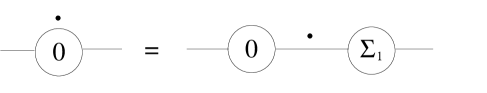
Figure 2: The Polchinski flow equation for the classical two-point vertex

If we concentrate just on the two-point vertex, diagrammatically the flow is of the form of fig. 2. It turns out that for the Polchinski equation one can set the classical two-point vertex equal to the seed action two-point vertex. Then the flow equation has a straightforward solution:

$$S_{0}^{\varphi\varphi}(p)=\hat{S}^{\varphi\varphi}(p)\implies\dot{S}^{\varphi\varphi}_{0}=-S_{0}^{\varphi\varphi}\dot{\Delta}S_{0}^{\varphi\varphi}\implies\Delta=\left(S_{0}^{\varphi\varphi}\right)^{-1},$$ (2.6)

so $\Delta$ is just the inverse of the classical effective action two-point vertex, justifying our naming it an effective propagator.

Later we will turn this analysis around, and insist that the classical and seed action two-point vertices can be identified and then the equation above determines what we use for the exact RG kernel, or equivalently the effective propagator. This step is not really necessary but it does lead to technical simplifications.

2.3 Generalised exact RG for a single scalar field

It is now straightforward to generalise this. For example we can replace the seed action by $\hat{S}=\frac{1}{2}\partial_{\mu}\varphi\cdot c^{-1}\cdot\partial_{\mu}\varphi+\cdots$, where the ellipses stands for some higher point vertices, or even an infinite number of higher point vertices. The only constraint, apart from the usual generic requirements, is that these vertices’ ultraviolet behaviour should not be so violent as to destroy the regularisation properties of $c$. In fact since the two-point vertex is the most general two-point vertex consistent with there being only one scale, $\Lambda$, and Poincaré invariance, in effect we replace the seed action by any effective action of our choice, as long as it corresponds to a regularised massless scalar field.

What changes? Hardly anything! The equation (2.5) and its diagrammatic interpretation, fig. 1, are still the same. The only difference is that one must remember that $\hat{S}$ vertices can now have more than two legs. It might seem surprising but the universal answers extracted from this equation are exactly the same as in standard quantum field theory. We have checked this explicitly. For example, for a single scalar field in four dimensions the first two beta function coefficients come out exactly the same, independent of the details of $c$ and the higher point vertices [29]. The underlying reason for this is that these extra terms amount to some reparametrisation of the field as the cutoff is lowered [10], and of course such a change of field variables does not change the physics.

3 Manifestly gauge invariant Exact RG for Yang-Mills

Replacing the scalar field $\varphi$ by a gauge field $A_{\mu}$, we can just require that the seed action is any choice of effective action: we do not even have to specify that the field is massless, since gauge invariance will ensure that. However making these simple replacements clearly does not turn (2.5) into a gauge invariant equation, because the gauge invariance is broken by the kernel. We can solve this problem by replacing $\dot{\Delta}(-\partial^{2}/\Lambda^{2})$ by $\dot{\Delta}(-D^{2}/\Lambda^{2})$. This is only one of infinitely many ways to covariantize a kernel. We will let braces stand for some fixed choice, which we will never have to specify precisely. Now the flow equation is gauge invariant:

$$\dot{S}={1\over 2}{\delta S\over\delta A_{\mu}}\{\dot{\Delta}\}{\delta\Sigma_{g}\over\delta A_{\mu}}-{1\over 2}{\delta\over\delta A_{\mu}}\{\dot{\Delta}\}{\delta\Sigma_{g}\over\delta A_{\mu}}.$$ (3.1)

It corresponds to the gauge covariant rate of change:

$$\Psi=\frac{1}{2}\,\{\dot{\Delta}\}\frac{\delta\Sigma_{g}}{\delta A_{\mu}}.$$

At the diagrammatic level, the only difference is that we have to remember that there are now fields hidden in the kernels, so the kernels themselves have vertices, as illustrated in fig. 3. One last detail: we scale the coupling constant out of the action, as in (1.1), and some thought shows that it ends up in front of the action so that in place of $\Sigma_{1}$ we have $\Sigma_{g}=g^{2}S-2\hat{S}$.

Figure 3: The flow equation in gauge theory.

Having scaled $g$ outside the action, we expect it to count powers of $\hbar$, and it is easy to check that (3.1) has this form for its weak coupling expansion:

$$S = {1\over g^{2}}S_{0}+S_{1}+g^{2}S_{2}+\cdots$$

$$\beta := \Lambda\partial_{\Lambda}g=\beta_{1}g^{3}+\beta_{2}g^{5}+\cdots,$$

where $S_{n}$ and $\beta_{n}$ are the $n$-loop pieces of the effective action and $\beta$ function respectively. Of course these components have yet to be computed.

3.1 Consequences at the classical level

Classical effective action vertices follow from the $g\to 0$ limit of (3.1), which is easily seen to be

$$\dot{S}_{0}={1\over 2}{\delta S_{0}\over\delta A_{\mu}}\{\dot{\Delta}\}{\delta\Sigma_{0}\over\delta A_{\mu}},\hskip 28.45274pt\hbox{where}\hskip 28.45274pt\Sigma_{0}=S_{0}-2\hat{S}.$$

Diagrammatically, this takes the form in fig. 4.

Figure 4: The classical flow equation for the classical part of the effective action.

Recall that we determine the kernel by insisting on the equality of the classical and seed action two-point vertices. The classical vertex has the following general form

$$S_{0\,\mu\nu}^{\phantom{0\,}AA}=\Box_{\mu\nu}(p)/c(p^{2}/\Lambda^{2}),\hskip 28.45274pt\hbox{where}\hskip 28.45274pt\Box_{\mu\nu}(p)=\delta_{\mu\nu}p^{2}-p_{\mu}p_{\nu}.$$

This form is fixed uniquely by masslessness, gauge invariance and Poincaré invariance. The arbitrary function $c$ will again play the rôle of a cutoff function. $\Box_{\mu\nu}(p)$ is the standard transverse kernel in the kinetic term of a gauge field. (From here on we suppress its dependence on $p$.) Since it has a longitudinal zero-mode: $\Box_{\mu\nu}p_{\nu}=0$, it is not invertible and this is the standard obstruction in gauge theory that motivates gauge fixing.

Following our procedure for determining the Exact RG kernel we see, using $\Box_{\mu\nu}\Box_{\nu\lambda}=p^{2}\Box_{\mu\lambda}$, that we get precisely the same solution for $\dot{\Delta}$ and thus also $\Delta$, as before:

$$S_{0\,\mu\nu}^{\phantom{0\,}AA}=\hat{S}^{AA}_{\mu\nu}\ \implies\ \dot{S}_{0\,\mu\nu}^{\phantom{0\,}AA}=-S_{0\,\mu\alpha}^{\phantom{0\,}AA}\dot{\Delta}S_{0\,\alpha\nu}^{\phantom{0\,}AA}\ \implies\ \Delta=c/p^{2}.$$

This satisfies

$$\Delta S_{0\,\mu\nu}^{\phantom{0\,}AA}=\delta_{\mu\nu}-p_{\mu}p_{\nu}/p^{2}.$$ (3.2)

Although we will keep calling $\Delta$ an effective propagator, it is not really an effective propagator any more because the two-point vertex has no inverse. Instead of unity on the RHS above, we get the transverse projector, or equivalently $\delta_{\mu\nu}$ minus the purely longitudinal term $p_{\mu}p_{\nu}/p^{2}$. This latter term when multiplying other elements in a diagram can be simplified by using the Ward identities that follow from invariance under small gauge transformations.

Specialising fig. 4 to the three-point vertex we get the diagrams in fig. 5.

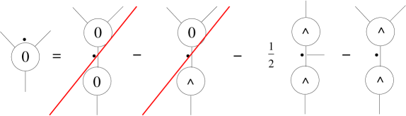
Figure 5: The flow equation for the classical three-point vertex. The seed-action vertices have a caret in the centre.

We now see the effect of covariantizing the kernel, in the third term on the RHS. The first two terms have the classical three-point vertex on the top, but they cancel because of the equality of classical and seed action two-point vertices. The remaining terms depend only on the covariantized kernel and seed action vertices, i.e. on terms that we put in by hand. Thus everything is known on the RHS and it easy to integrate this with respect to RG time to get the full classical three-point vertex. Notice that we have computed this without having to try to invert the (non-invertible) kinetic term.

This cancellation works for all the other vertices at the classical level: the flow is only into terms that have already been determined. For example, the flow of the four-point vertex is shown in fig. 6.

Figure 6: The flow equation for the classical four-point vertex.

On the RHS there are non-vanishing terms with effective action vertices this time, but these are the three-point vertices that we have just determined. Therefore this equation is straightforward to integrate, giving the four-point vertex. In the same way we can determine all the vertices at the classical level.

3.2 One loop

Let us illustrate what happens at one loop by considering just one particular piece – the part that yields the famous asymptotically free $\beta$ function for the coupling constant $g$. Recall that it is defined through the renormalization condition (1.1). This tells us that the two-point vertex $S_{\mu\nu}(p)=\Box_{\mu\nu}/g^{2}+O(p^{4})$, where the higher powers of momentum come exclusively from the higher dimension operators. Therefore when we compute the flow of $S_{\mu\nu}(p)$ at $O(p^{2})$, all we pick up is the flow of $g$, i.e. the $\beta$ function. At one loop, from (3.1), we find

$$-2\beta_{1}\Box_{\mu\nu}(p)+O(p^{4})=\left.\frac{1}{2}\frac{\delta}{\delta A_{\alpha}}\{\dot{\Delta}\}\frac{\delta\Sigma_{0}}{\delta A_{\alpha}}\right|^{AA}_{\mu\nu},$$ (3.3)

which, when expanded, gives the diagrams of fig. 7.

Figure 7: Two-point vertex at one loop and $O(p^{2})$.

However, when we compute these diagrams we find that the integrals do not converge. The ultraviolet divergences are not regulated. This is not a surprise. Covariantizing the cutoff function in the way that we have done is equivalent to implementing a covariant higher derivatives regularisation and this is known to fail, precisely at one loop [30].

We have to replace this effective covariant higher derivatives with some other gauge invariant regularisation which can naturally be incorporated in this Exact RG framework, such that it cures this problem. One way to proceed is to add covariant Pauli-Villars fields [31] in such a way to as to cancel the leading divergences. This leads to further divergences which one cancels by introducing new regulator fields and interactions. Continuing in this way one finds eventually that the whole framework closes; the interactions are essentially unique and once in place, all diagrams, including the new ones, are regularised .

After staring at the result for a while, one realises that there is a much more elegant way to arrive at the same answer [16, 17, 18, 19].

4 $SU(N|N)$ regularisation

4.1 $SU(N|N)$ Yang-Mills

Take the $SU(N)$ Yang-Mills and embed $SU(N)$ in the supergroup $SU(N|N)$. Its Lie algebra is realised by supermatrices, which we employ in the defining representation. The gauge field becomes a supergauge field,

$$\mathcal{A}_{\mu}=\left(\!\!\begin{array}[]{cc}A^{1}_{\mu}&B_{\mu}\\ \bar{B}_{\mu}&A^{2}_{\mu}\end{array}\!\!\right)+{\mathcal{A}}^{0}_{\mu}\hbox{1\kern-2.27621ptl},$$

where $A^{1}$ and $A^{2}$ are traceless Hermitian matrices and the off-diagonal terms $B$ and $\bar{B}$, are Grassmann valued, and thus anticommuting (fermionic). It turns out we also have to add the $\mathcal{A}^{0}$ term, proportional to the $2N\times 2N$ unit matrix.

$A^{1}$ gauges the original $SU_{1}(N)$ group. We add an index to the group to distinguish it from an extra copy, $SU_{2}(N)$, gauged by $A^{2}$. The bosonic subgroup is therefore $SU_{1}(N)\otimes SU_{2}(N)\otimes U(1)$, where the $U(1)$ factor is carried by $\mathcal{A}^{0}$. If we had been dealing with a compact Lie algebra, as is normally used in gauge theory, we would be able to discard this $U(1)$ factor, but we cannot here because the $SU(N|N)$ superalgebra is an example of an indecomposable superalgebra; $\mathcal{A}^{0}$ gauges a central term produced by some of the fermionic generators, for example:

$$\left\{\left(\begin{array}[]{cc}0&\hbox{1\kern-2.27621ptl}\\ \hbox{1\kern-2.27621ptl}&0\\ \end{array}\right),\left(\begin{array}[]{cc}0&\hbox{1\kern-2.27621ptl}\\ \hbox{1\kern-2.27621ptl}&0\\ \end{array}\right)\right\}=2\hbox{1\kern-2.27621ptl}.$$

This leads to some technicalities which are nevertheless key, so we briefly describe them. To form invariants we must use the supertrace

$$\mathrm{str}\left(\begin{array}[]{cc}X^{11}&X^{12}\\ X^{21}&X^{22}\\ \end{array}\right)={\mathrm{tr}}_{1}X^{11}-{\mathrm{tr}}_{2}X^{22},$$ (4.1)

because it is this that is cyclically invariant for supermatrices and thus this which leads to the construction of $SU(N|N)$ invariants. The action will thus be built from a supercovariant derivative $\nabla_{\mu}=\partial_{\mu}-i\mathcal{A}_{\mu}$ as

$$S\sim{1\over 4g^{2}}\ \mathrm{str}\!\int\!\mathcal{F}^{2}_{\mu\nu}.$$ (4.2)

This has a neat effect on the central term because the kinetic term for $\mathcal{A}^{0}$ will just be a $U(1)$ field strength squared times $\mathrm{str}\hbox{1\kern-2.27621ptl}$. But from (4.1), $\mathrm{str}\hbox{1\kern-2.27621ptl}=N-N=0$. Therefore $\mathcal{A}^{0}$ has no kinetic term. Furthermore, its interactions are formed from commutators, but 1l commutes with everything and thus $\mathcal{A}^{0}$ has no interactions. It therefore does not appear at all in the action displayed above.

We now raise this to a principle and require that the theory be invariant under the local shift symmetry

$$\delta\mathcal{A}^{0}_{\mu}=\lambda_{\mu}(x).$$ (4.3)

This “no-$\mathcal{A}^{0}$ symmetry” simply ensures that nothing in fact depends on $\mathcal{A}^{0}$. It means that in practice we gauge the coset space $SU(N|N)/U(1)$.

The $SU(N|N)/U(1)$ theory has very nice properties at high momenta. In particular one can show that the quadratic Casimir vanishes, which it turns out is sufficient to ensure that the effective action is finite at one loop. At higher loops, wherever the $SU(N)$ theory yielded ${\mathrm{tr}}\hbox{1\kern-2.27621ptl}=N$, one now obtains $\mathrm{str}\hbox{1\kern-2.27621ptl}=0$, thus in the ’t Hooft large $N$ limit this theory has no quantum corrections at all.

Note that there is no sense in which this can be regarded as a physical theory, in particular the $B_{\mu}$ are fermionic integer spin particles which thus violate Pauli’s spin statistics theorem [32]. The kinetic term for $A^{2}$ has the wrong sign, as follows from (4.2) and (4.1). This leads to negative norm states in the Fock space [17]. However we will be able to ensure that these sicknesses are felt by the physical $SU(N)$ Yang-Mills sector only at the cutoff scale.

4.2 $SU(N|N)$ $\rightarrow$ $SU_{1}(N)\otimes SU_{2}(N)$ spontaneous breaking

At high energies this more symmetric theory has some very useful ultraviolet properties. At low energies we want to recover just the $SU(N)$ Yang-Mills. In particle physics we know how to go from one regime to the other: we use the Higgs mechanism. We therefore introduce a super-Higgs field, the superscalar

$$\mathcal{C}=\left(\!\!\begin{array}[]{cc}C^{1}&D\\ \bar{D}&C^{2}\end{array}\!\!\right),$$

the $C^{i}$ being bosonic and the off-diagonal $D$ being fermionic. We can arrange a potential so that $\mathcal{C}$ picks up the expectation value

$$\langle\mathcal{C}\rangle=\Lambda\left(\begin{array}[]{cc}\hbox{1\kern-2.27621ptl}&0\\ 0&-\hbox{1\kern-2.27621ptl}\\ \end{array}\right).$$ (4.4)

It is easy to show that this Pauli $\sigma_{3}$-matrix form breaks spontaneously all the fermionic directions, and only the fermionic directions. Thus, via the Higgs mechanism, the $B$s eat the $D$s and they become massive with masses of order the cutoff, where we will ultimately be able to ignore them. The ‘physical’ Higgs fields $C^{i}$ can also be given masses at the cutoff scale, so all that remains at low energies are the two massless gauge fields $A^{1}$ and $A^{2}$. However in this gauge invariant approach, because the gauge fields are charged under different groups, the lowest dimension interaction between them is

$${1\over\Lambda^{4}}\ {\mathrm{tr}}_{1}\left(F^{1}_{\mu\nu}\right)^{2}{\mathrm{tr}}_{2}\left(F^{2}_{\mu\nu}\right)^{2}.$$

This is already dimension 8, so by the Symanzik-Appelquist-Carazzone theorem [33] the two sectors decouple into a direct product in the low energy limit.

At finite $N$, and with this extra $\mathcal{C}$ sector, we need to supply some covariantized cutoff functions in order to make the theory ultraviolet finite. It is then possible to show this to all orders in perturbation theory. For completeness we give the precise statement and sketch the steps necessary to prove it [17].

Theorem 4.1.

Let

$$S=\mathrm{str}\int{1\over 4g^{2}}\mathcal{F}_{\mu\nu}c^{-1}\left(-{\nabla^{2}\over\Lambda^{2}}\right)\mathcal{F}_{\mu\nu}+\frac{1}{2}\nabla_{\mu}\mathcal{C}\,{\tilde{c}}^{-1}\left(-{\nabla^{2}\over\Lambda^{2}}\right)\nabla_{\mu}\mathcal{C}+{\lambda\over 4}\left(\mathcal{C}^{2}-\Lambda^{2}\right)^{2},$$

where $c^{-1}$ is a polynomial of rank $r$ and ${\tilde{c}}^{-1}$ is a polynomial of rank ${\tilde{r}}$. Shifting $\mathcal{C}\mapsto\mathcal{C}+\Lambda\left(\begin{array}[]{cc}\hbox{1\kern-2.27621ptl}&0\\ 0&-\hbox{1\kern-2.27621ptl}\\ \end{array}\right)$, all amplitudes are finite to all orders in perturbation theory providing $r>{\tilde{r}}+1$ & ${\tilde{r}}>1$.

We use standard techniques of perturbative field theory for the proof, to avoid confusing the issue of regularisation with those of manifest gauge invariance and the Exact RG description. The first step therefore is to gauge fix to ’t Hooft gauge. We introduce a further cutoff function ${\hat{c}}^{-1}$ (rank ${\hat{r}}$) for the gauge fixing term and thus also the BRST ghosts. Providing that ${\hat{r}}\geq r>{\tilde{r}}-1$ and ${\tilde{r}}>-1$ the leading contributions at high momentum have the symmetries of the symmetric regime. By power counting, one can show that if ${\hat{r}}\geq r$, $r-{\tilde{r}}>1$ and ${\tilde{r}}>1$, all diagrams are superficially finite except certain “remainder contributions”: symmetric phase parts of one-loop graphs with no external $\mathcal{C}$ or ghost lines and up to four external $\mathcal{A}$s. Of these, two-point and three-point diagrams vanish by properties of the superalgebra since one can show that they involve only the following forms: $\mathrm{str}\mathcal{A}\,\mathrm{str}\mathcal{A}$, $\mathrm{str}\mathcal{A}\mathcal{A}\,\mathrm{str}\hbox{1\kern-2.27621ptl}$, $\mathrm{str}\mathcal{A}\mathcal{A}\,\mathrm{str}\mathcal{A}$ and $\mathrm{str}\mathcal{A}^{3}\,\mathrm{str}\hbox{1\kern-2.27621ptl}$. These all vanish because $\mathrm{str}\hbox{1\kern-2.27621ptl}=0$ and $\mathrm{str}\mathcal{A}=0$. This leaves only the symmetric phase four-point diagram which can be proved to be finite by Lee-Zinn-Justin identities [13]. The result is only conditionally convergent. This can be made well defined by an appropriate limiting procedure. Defining the theory in dimension $D\to 4^{-}$ is sufficient.

5 Manifestly $SU(N|N)$ gauge invariant Exact RG

We now combine the ideas in the last two sections. Given the field content, this amounts to finding an appropriate choice for $\Psi$ in (2.2).

$$\dot{S} = {1\over 2}{\delta S\over\delta\mathcal{A}_{\mu}}\{\dot{\Delta}^{\mathcal{A}}\}{\delta\Sigma_{g}\over\delta\mathcal{A}_{\mu}}+{1\over 2}{\delta S\over\delta\mathcal{C}}\{\dot{\Delta}^{\mathcal{C}}\}{\delta\Sigma_{g}\over\delta\mathcal{C}}$$

$$+ {1\over 2}[\mathcal{C},{\delta S\over\delta\mathcal{A}_{\mu}}]\{\dot{\Delta}^{\mathcal{A}}_{m}\}[\mathcal{C},{\delta\Sigma_{g}\over\delta\mathcal{A}_{\mu}}]+{1\over 2}[\mathcal{C},{\delta S\over\delta\mathcal{C}}]\{\dot{\Delta}^{\mathcal{C}}_{m}\}[\mathcal{C},{\delta\Sigma_{g}\over\delta\mathcal{C}}]$$

$$+ {1\over 2}{\delta S\over\delta\mathcal{A}_{\mu}}\{\dot{\Delta}^{\mathcal{A}}_{\sigma}\}\left(\{\mathcal{C},{\delta\Sigma_{g}\over\delta\mathcal{A}_{\mu}}\}\,\mathrm{str}\,\mathcal{C}-2\mathcal{C}\,\mathrm{str}\left\{\mathcal{C}{\delta\Sigma_{g}\over\delta\mathcal{A}_{\mu}}\right\}\right)\ +\left(S\leftrightarrow\Sigma_{g}\right)$$

$$+ \ \hbox{quantum terms}.$$

On the first line we have the term expected already which gives the flow equation for the gauge (now supergauge) field, together with its kernel which we have yet to determine. We also have a piece for the super-Higgs and its corresponding kernel. The whole flow equation must be invariant under

$$\delta\mathcal{C}=-i[\mathcal{C},\Omega],\quad\delta\mathcal{A}_{\mu}=[\nabla_{\mu},\Omega]+\lambda_{\mu}\hbox{1\kern-2.27621ptl},\quad\delta\!\left({\delta\over\delta\mathcal{A}_{\mu}}\right)=-i\left[{\delta\over\delta\mathcal{A}_{\mu}},\Omega\right]+{\tilde{\lambda}}_{\mu}\hbox{1\kern-2.27621ptl},$$ (5.2)

i.e. the combination of $SU(N|N)$ supergauge transformations, and the no-$\mathcal{A}^{0}$ symmetry that ensures we divide out by the central term. The top line is already invariant under these but it is not enough because we want to keep the technical simplifications that follow from setting the classical two-point vertex equal to the seed action two-point vertex. This means that in the spontaneously broken phase we have to allow the kernels for the fermionic fields to grow a mass term, because the corresponding effective propagators must be inverses of their now-massive two-point vertices. The simplest such terms are displayed on the second line of (5): using (4.4), the commutators isolate (at the two-point level) just the fermionic directions as required. We are not quite done yet. We have to remember that really we now have two coupling constants, one for our original gauge field $A^{1}$ and one for the unphysical copy $A^{2}$. At the quantum level we can no longer identify the two couplings because the wrong sign action for $A^{2}$ results in its coupling running with the wrong sign. (It is asymptotically trivial rather than asymptotically free.) In the way we are doing things, this changes the normalisation of the $A^{2}$’s kinetic term. Thus, if we are to keep the equality of $\hat{S}$ and $S_{0}$ two-point vertices we have to allow for different effective propagators for the two gauge fields. The simplest term that allows for this in the flow equation, whilst still obeying the symmetries (5.2), is the multi-supertrace term on the third line of (5). Finally the quantum terms are just analogous to the last term in (3.1), as determined by the general form (2.2).

(One can further understand the appearance of these multisupertrace terms as follows. Classically the effective action contains the terms:

$$S_{0}={1\over 4g^{2}}\ \mathrm{str}\int\left(\begin{array}[]{cc}\left(F^{1}_{\mu\nu}\right)^{2}&0\\ 0&\left(F^{2}_{\mu\nu}\right)^{2}\\ \end{array}\right)+\cdots.$$

Since the one-loop correction has opposite sign for $A^{2}$, it takes the form

$$-{\beta_{1}\over g^{2}}\ \ln{\Lambda\over\mu}\ \mathrm{str}\left(\begin{array}[]{cc}\hbox{1\kern-2.27621ptl}&0\\ 0&-\hbox{1\kern-2.27621ptl}\\ \end{array}\right)\left(\begin{array}[]{cc}\left(F^{1}_{\mu\nu}\right)^{2}&0\\ 0&\left(F^{2}_{\mu\nu}\right)^{2}\\ \end{array}\right).$$

At first sight such a correction is a puzzle since naïve guesses for the full contribution as a functional of $\mathcal{A}$, do not obey the no-$\mathcal{A}^{0}$ symmetry. In fact, as we confirmed by direct calculation, this term arises from a contribution of the form

$$\mathrm{str}\,\mathcal{C}\,\mathrm{str}\,\mathcal{C}\mathcal{F}_{\mu\nu}^{2}-\left(\mathrm{str}\,\mathcal{C}\mathcal{F}_{\mu\nu}\right)^{2}|_{\mathcal{C}\to\mathcal{C}+\Lambda\sigma_{3}}+\cdots,$$

where the ellipses stands for higher dimension invariant terms. This does obey no-$\mathcal{A}^{0}$ symmetry as can be seen by using $\delta\mathcal{F}_{\mu\nu}=(\partial_{\mu}\lambda_{\nu}-\partial_{\nu}\lambda_{\mu})\hbox{1\kern-2.27621ptl}.$ The terms we added in the flow equation have a similar structure and indeed allow contributions such as above to be incorporated at tree-level, as now required.)

5.1 The kernels

The kernels in (5) are determined in the same way as before. We first write down the classical two-point vertices in a form as general as required and such that they are consistent with broken supergauge invariance and the renormalization conditions (and Poincaré invariance etc.). We then insist that the $\hat{S}$ two-point vertices are equal to these and this determines the kernels. For example, the two-point classical flow equations for the gauge fields take the form

$$\dot{S}_{0\,\mu\nu}^{\phantom{0\,}A_{1}A_{1}}=-S_{0\,\mu\alpha}^{\phantom{0\,}A_{1}A_{1}}\dot{\Delta}^{1}S_{0\,\alpha\nu}^{\phantom{0\,}A_{1}A_{1}}\hskip 28.45274pt\hbox{and}\hskip 28.45274pt\dot{S}_{0\,\mu\nu}^{\phantom{0\,}A_{2}A_{2}}=-S_{0\,\mu\alpha}^{\phantom{0\,}A_{2}A_{2}}\dot{\Delta}^{2}S_{0\,\alpha\nu}^{\phantom{0\,}A_{2}A_{2}},$$

determining $\Delta^{1}$ and $\Delta^{2}$, which are the linear combinations $\Delta^{1}=\Delta^{\mathcal{A}}+8N\Delta^{\mathcal{A}}_{\sigma}$ and $\Delta^{2}=\Delta^{\mathcal{A}}-8N\Delta^{\mathcal{A}}_{\sigma}$. In the same way, the other two-point classical flow equations determine linear combinations of the original kernels, and inverting we finally find expressions for the original kernels. The superscalar field classical two-point vertex flows in the same way as the scalar field considered earlier:

$$\dot{S}_{0}^{CC}=-S_{0}^{CC}\dot{\Delta}^{C}S_{0}^{CC}.$$

However, the $B$ and $D$ fields mix which other. This is just the Higgs effect in this manifestly gauge invariant description. We therefore use $2\times 2$ matrices to describe the flow:

$$\left(\!\!\begin{array}[]{cc}\dot{S}_{0\,\mu\nu}^{\phantom{0\,}\bar{B}B}&\!\!\!\dot{S}_{0\,\mu}^{\phantom{0\,}\bar{B}D}\\ -\dot{S}_{0\,\nu}^{\phantom{0\,}\bar{B}D}&\!\!\!-\dot{S}^{\bar{D}D}_{0}\\ \end{array}\!\!\right)=-\left(\!\!\begin{array}[]{cc}S_{0\,\mu\alpha}^{\phantom{0\,}\bar{B}B}&\!\!\!S_{0\,\mu}^{\phantom{0\,}\bar{B}D}\\ -S_{0\,\alpha}^{\phantom{0\,}\bar{B}D}&\!\!\!-S^{\bar{D}D}_{0}\\ \end{array}\!\!\right)\left(\!\!\begin{array}[]{cc}\dot{\Delta}^{B}\delta_{\alpha\beta}&0\\ 0&\!\!\!\!\!\!-\dot{\Delta}^{D}\\ \end{array}\!\!\right)\left(\!\!\begin{array}[]{cc}S_{0\,\beta\nu}^{\phantom{0\,}\bar{B}B}&\!\!\!S_{0\,\beta}^{\phantom{0\,}\bar{B}D}\\ -S_{0\,\nu}^{\phantom{0\,}\bar{B}D}&\!\!\!-S^{\bar{D}D}_{0}\\ \end{array}\!\!\right).$$

A much more elegant description involves combining these into five-dimensional fields but for simplicity we will not do so here.

5.2 Effective propagator relations

From the above flow equations we determine the effective propagators and thus get a relation of the same form as (2.6):

$$S_{0}^{CC}\Delta^{C}=1,$$

and relations analogous to (3.2):

$$S_{0\,\mu\ \nu}^{\phantom{0}A_{1}\!A_{1}}\Delta^{1}=\delta_{\mu\nu}-p_{\mu}p_{\nu}/p^{2}\hskip 28.45274pt\hbox{and}\hskip 28.45274ptS_{0\,\mu\ \nu}^{\phantom{0}A_{2}\!A_{2}}\Delta^{2}=\delta_{\mu\nu}-p_{\mu}p_{\nu}/p^{2}.$$

Once again, the effective propagators here are not really propagators: multiplying the two-point vertex they give unity up to terms that simplify via gauge transformations. For the $B$s and $D$s one finds

$$\left(\!\!\begin{array}[]{cc}S_{0\,\mu\alpha}^{\phantom{0\,}\bar{B}B}&\!\!\!S_{0\,\mu}^{\phantom{0\,}\bar{B}D}\\ -S_{0\,\alpha}^{\phantom{0\,}\bar{B}D}&\!\!\!-S^{\bar{D}D}_{0}\\ \end{array}\!\!\right)\left(\!\!\begin{array}[]{cc}\Delta^{B}\delta_{\alpha\nu}&0\\ 0&\!\!\!\!\!\!-\Delta^{D}\\ \end{array}\!\!\right)=\left(\!\!\begin{array}[]{cc}\delta_{\mu\nu}&0\\ 0&1\\ \end{array}\!\!\right)-\left(\!\!\begin{array}[]{c}f{p_{\mu}\over\Lambda^{2}}\\ g\\ \end{array}\!\!\right)\left(p_{\nu}\ 2\right).$$

This is unity up to a term which simplifies using spontaneously broken supergauge transformations: the $(p_{\nu}\ 2)$ part operating on a vertex can be simplified via broken Ward identities. Its coefficient contains the cutoff dependent terms $f_{p}$ and $g_{p}$, whose precise structure depends on the parameterisation we used for the two-point vertices [19]. We can unify all of these relations diagrammatically as in fig. 8. We write the coefficient parts as a single unfilled arrow i.e. as “${\color[rgb]{1,0,0}>}$” and fill this arrow in when we include also the terms that generate gauge transformations (null, $p_{\nu}$ and $(p_{\nu}\ -2)$ for the $C$, $A$ and $B/D$ sectors respectively). Then in all sectors, the two-point classical action (or seed action) vertex attached to an effective propagator gives 1 minus a term which simplifies on using Ward identities.

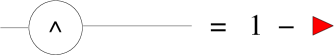
Figure 8: Diagrammatic representation of the effective propagator relations.

5.3 ‘Naïve’ Ward identities

To see what these Ward identities look like, it is enough to consider the simple case in pure $SU(N)$ gauge theory of a vertex of the form

$$S={\cdots+}\int S_{\mu_{1}\mu_{2}\cdots\mu_{n}}(p_{1},p_{2},\cdots,p_{n})\,{\mathrm{tr}}\,A_{\mu_{1}}(p_{1})A_{\mu_{2}}(p_{2})\cdots A_{\mu_{n}}(p_{n})\ \ {+\cdots}.$$

This is because the diagrammatic representation turns out to be the same for any vertex in all sectors [20, 21, 22]. Requiring that the action be invariant under infinitessimal gauge transformations (1.2), i.e. $\delta A_{\mu}=\partial_{\mu}\omega-i[A_{\mu},\omega]$, results in the so-called naïve Ward identities:

$$p_{1}^{\mu_{1}}S_{\mu_{1}\mu_{2}\cdots\mu_{n}}(p_{1},p_{2},\cdots,p_{n})=\phantom{S_{\mu_{1}\mu_{2}\cdots\mu_{n}}(p_{1},p_{2},\cdots,p_{n})}$$

$$\phantom{S_{\mu_{1}\mu_{2}\cdots\mu_{n}}()}S_{\mu_{2}\cdots\mu_{n}}(p_{1}\!+\!p_{2},p_{3},\cdots,p_{n})-S_{\mu_{2}\cdots\mu_{n}}(p_{2},p_{3},\cdots,p_{n}\!+\!p_{1}).$$

They are called “naïve” because in the gauge fixed approach one should really be using BRST invariance which leads to complications and ultimately the Lee-Zinn-Justin identities [14, 13]. Here, because the gauge invariance is preserved we get the above simple form. (The commutator part of the non-Abelian gauge transformation provides the RHS which would just be zero in an Abelian gauge theory.) In the diagrammatic representation we see that the contraction of the term generating gauge transformations results in the momentum of that leg being ‘pushed forward’ onto the following leg (with a plus sign) or ‘pulled back’ onto the previous leg (with a minus sign) as illustrated in fig. 9.

Figure 9: Diagrammatic representation of the Ward identities. Only one push-forward (counterclockwise arrow) and pull-back (clockwise arrow) have been drawn. By symmetry they appear on all legs of the vertex.

In fact, since the vertex has been symmetrised over permutations (as usual in Feynman diagrams), the pull-backs and push-forwards operate on all legs.

6 Diagrammatic Method

We now have all the elements necessary to describe the full diagrammatic method. The flow equation has the same diagrammatic form as before, viz. fig. 3. All we have to remember, in fact most of the time we can forget, is that propagating between vertices is now not just the gauge field $A^{1}$ but all the other partners ($A^{2}$, $B$, $C$, $D$), which are necessary for regularisation. This means only that internal legs (kernels or effective propagators) must be interpreted as summed over these flavours.

As a consequence the one-loop diagrams look the same as before, viz. fig. 7, however these diagrams converge, not only in the infrared (as guaranteed by the Wilsonian formalism for smooth cutoffs) but also now in the ultraviolet. Therefore, we can just compute them. However we want to proceed without having to specify the regularisation structure (cutoff functions, covariantization, and seed action) precisely. This leaves us with very little room to maneouver. The only worthwhile operation is to shift the RG-time derivative in the first diagram by integration by parts, resulting in fig. 10.

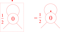
Figure 10: Shifting the RG-time derivative. The differential is now outside the integral in the first expression.

Since the integral in the first diagram is a contribution to the $\beta$ function, it is dimensionless. A priori the integral can depend only upon $\Lambda$. However, since $\Lambda$ has dimensions of mass and there is no other dimensionful parameter, the integral is in fact independent of this and is thus a pure number. Differentiating it gives zero.

We have thus effectively shifted the RG-time derivative onto the classical vertex, as in the remaining diagram of fig. 10. We can now expand this flow using fig. 6. This results in a bunch of diagrams, corresponding to all possible ways of tieing up two legs in the diagrams on the RHS of fig. 6. Let us concentrate on just two of these. The first diagram displayed in fig. 11 corresponds to tieing up a top and a bottom leg from the first diagram on the RHS of fig. 6.

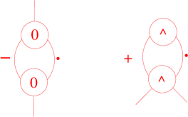
Figure 11: Examples of diagrams obtained from expanding the second diagram in fig. 10, together with their combinatorics.

The second diagram in fig. 11, the result of tieing up the top and bottom legs of the third diagram on the RHS of fig. 6, can be processed further. We use the effective propagator relations, fig. 8. The result is fig. 12.

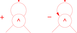
Figure 12: The result of applying effective propagator relations to the second diagram in fig. 11.

The first diagram in this figure is equal and opposite to the second diagram in the original list, fig. 7, so that now two diagrams have disappeared from this list. The second diagram in fig. 12 can be processed further by using the Ward identities, fig. 9, pushing-forwards and pulling-backwards to give fig. 13.

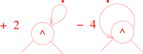
Figure 13: The result of applying the Ward identities to the second diagram in fig. 12.

We continue to proceed in the same way, for example the first diagram of fig. 11 can be expressed as a total derivative minus terms where the RG-time derivative hits the classical three-point vertices. These can thus be expanded. Evaluating these and others in the same way, we find that all diagrams cancel, including the originals in fig. 7, except for the set of total derivative diagrams in fig. 14 [20, 21].

Figure 14: The final diagrams contributing the one-loop $\beta$ function.

(The third diagram is the result of expanding to $O(p^{2})$, as required from (3.3), and processing the resulting derivatives with respect to $p^{\lambda}$ using differential Ward identities [20, 21].)

We saw in fig. 10 that the total RG-time derivative of a diagram contributing to $\beta$ is zero because the integral can only give a pure number. The only reason that these diagrams are not also zero is that in the exchange of limits, placing the differential with respect to RG-time outside the momentum integral, we have introduced infrared divergences. In other words, strictly speaking we were not allowed to exchange limits in this way, however doing so has the advantage that we see very clearly that the results for these integrals depend only on the massless fields (i.e. the $A^{i}$) propagating in the far infrared. For such vanishing momenta, all the elements in the integral are then determined by the renormalization conditions. That is why the result is universal. It is easy to compute the resulting integrals, and thus we obtain [21, 19]:

$${22N\over 3(4\pi)^{2}}\,\Box_{\mu\nu}(p)+O(p^{4}).$$

By comparing to our starting point, (3.3), we extract the famous asymptotically free one-loop beta function for Yang-Mills.

The procedure generalises to two loops and beyond. The main new feature is that subtraction diagrams need to be defined in order to isolate the universal parts [20, 23]. In this way, we have confirmed that the universal two-loop beta function is also reproduced by these methods.

7 QCD

Spinors transforming in the fundamental representation can be incorporated in the framework, so we can compute in the physically important theory of Quantum Chromodynamics, without fixing the gauge [34]. These fermions are the quarks; the gauged group is $SU(3)$; $A^{1}$ is thus the gluon field.

The obvious thing to try, is to extend the quark spinor $\psi$ to a fundamental representation $\Psi$ of $SU(3|3)$. However, gauge invariance then fixes the interaction to be of the form $\Psi\mathcal{A}\!\!\!/\Psi$ which violates the no-$\mathcal{A}^{0}$ invariance (4.3). The only way out is to try a different embedding which does not have this problem. In fact we can embed $\psi$ in the off-diagonal part of a $3\times 3$ supermatrix (transforming as a complexified $U(3|3)$ adjoint field):

$$\Psi=\left(\begin{array}[]{cc}\varphi^{1}&\psi\\ \varrho&\varphi^{2}\\ \end{array}\right).$$

In this way $\psi$ is fermionic by default. It transforms as the fundamental under colour, $SU_{1}(3)$, and complex conjugate fundamental under $SU_{2}(3)$. Thus we are forced into a situation where $\Psi$ represents multiples of three flavours of quark. From this point of view it is at least serendipitous that nature decided that as well as three colours, there are also three families. One super-spinor $\Psi_{u}$ can thus contain the up-type quarks $u$, $c$ and $t$, and another super-spinor $\Psi_{d}$ hold the down-type quarks $d$, $s$ and $b$. Of course at this stage the family symmetry $SU_{2}(3)$ is gauged, moreover by the unphysical field $A_{2}$. To give the quarks different masses, we need to break it spontaneously (so that we keep the regularising properties of $SU(3|3)$ at high energies).

(Although it is cute that families come in multiples of the number of colours, there is no restriction to handling different numbers of families since we can always send individual quark masses to infinity at the end of the calculation.)

8 Other applications

We note that these ideas have been generalised, or rather simplified, to the case of QED [35], and the steps necessary for computing general gauge invariant matrix elements have also been fleshed out and incorporated in this general scheme, using the example of the one-loop contribution to the Wilson loop [26]. We were also able to use these ideas to make explicit the cutoff in the AdS/CFT construction [36].

So far we have only discussed explicitly the perturbative expansion of the flow equations, and concentrated on the evaluation of the first two $\beta$ function coefficients, without gauge fixing. The fact that this all works however, gives us experience and confidence in applying the framework to the non-perturbative regime. As we intimated in the introduction, there is a wide variety of possible approximations that can be applied.

Indeed within this framework, we have already studied the large $N$ approximation to some extent in [15]. The similarities to string theory that this uncovered, together with the gauge (and Poincaré) invariant cutoff definition in this framework, and suggestions of exact RG from the AdS/CFT side [37], provided the initial motivation to search for some connection with the AdS/CFT construction.

We would also like to mention that it is possible to perform a sort of Eguchi-Kawai reduction [38] of the equations, this time in the continuum, casting the equations in an equivalent way in terms of vertices that carry no momentum [39].

Of course one can also simply resort to truncations, a strategy that has been very popular in the exact RG field [4, 5].

We would like to finish by showing that under some very general conditions, confinement is a natural consequence in this framework [39]. We then describe in some detail one further possibility adapted to this observation, namely a strong renormalized coupling expansion, which indeed could be combined with any of the above approaches and could have more general applicability to other exact RGs [39]. As well as being a desirable starting point for further approximation, it means that one can test for confinement within this framework by instead testing whether these general conditions hold true or not.

9 Confinement

From the perturbative $\beta$ function we know that $g(\Lambda)$ grows as $\Lambda$ gets smaller. Although we cannot trust perturbation theory in this regime, the natural expectation is that $g$ grows without limit. Indeed in any formulation where the gauge invariance is manifest, including lattice gauge theory, the gluon itself cannot have a mass gap. Intuitively, in this case confinement only follows if the coupling diverges in the infrared. (In the gauge fixed theory, arguments based on the Kugo-Ojima criterion [40] actually come to the opposite conclusion: that $g$ freezes out at some finite value. There is some evidence for this in gauge fixed formulations [41], however these arguments depend by their very nature on the ghost fields and thus have nothing to say about a manifestly gauge invariant approach. In any case, a priori both pictures can be correct since they refer to different non-perturbative definitions of $g$.)

Our first condition then is that $g(\Lambda)\to\infty$ as $\Lambda$ decreases. In principle, we could find that $g$ diverges at a finite critical value $\Lambda\to\Lambda_{cr}>0$ but in this case we would have an obstruction to completing the computation in this way, which requires that we integrate out all the modes, i.e. that we take the limit $\Lambda\to 0$. It may be that a change of variables will allow us to pass smoothly over $\Lambda_{cr}$, i.e. that the problem is a kind of ‘coordinate singularity’. If this can be done in terms of some $SU(N|N)$ fields $\mathcal{A}$ and $\mathcal{C}$, it amounts to a different choice for $\Psi$ in (2.2), i.e. a different choice of exact RG.

Therefore we require that $g(\Lambda)\to\infty$, but only as $\Lambda\to 0$; we require this for at least one of the infinitely many choices that we have for gauge invariant exact RGs, if we are to find confinement in this framework.

Remember that $g$ is defined by the renormalization condition (1.1), which tells us that the effective two-point $A^{1}$ vertex has the form

$$S_{\mu\nu}(p)=\Box_{\mu\nu}(p)/g^{2}+O(p^{4}).$$ (9.1)

It follows that in this case, in the limit $\Lambda\to 0$ we find $S_{\mu\nu}(p)\sim O(p^{4})$. This is a well-known signal of confinement. Indeed the three dimensional Fourier transform of the (gauge fixed) full effective propagator gives the effective potential $V(r)$ between two colour charges. In the perturbative regime one has for large $r$, the standard Coulomb potential, as follows trivially from dimensional analysis:

$$V(r)\sim\int{d^{3}p\over p^{2}}\,\,{\rm e}^{\displaystyle i{\bf p}\!\cdot\!{\bf r}}\sim{1\over r}.$$

In this non-perturbative regime we have instead the famous linearly rising form for large $r$, corresponding to a constant Yang-Mills string tension and confinement:

$$V(r)\sim\int{d^{3}p\over p^{4}}\,\,{\rm e}^{\displaystyle i{\bf p}\!\cdot\!{\bf r}}\sim r,$$

as again follows trivially by dimensional analysis. In what amounts to much the same computation, one can show that changing the propagator from $1/p^{2}$ to $1/p^{4}$ changes the lowest order contribution to the expectation value of a Wilson loop from perimeter law to area law (another standard signal of confinement).

We therefore come to the conclusion that in this manifestly gauge invariant exact RG formalism, confinement occurs if and only if $g(\Lambda)\to\infty$ as $\Lambda\to 0$.

10 Renormalized strong coupling expansion

Although this observation is neat, we cannot use it as a basis for computation in this regime because it only makes sense for momentum $p\approx 0$ (which is in fact all that is needed to confirm the form of the potentials above for large $r$). The reason is as follows. Since we are dealing with a continuum limit the effective action must be in self-similar form (cf. the introduction), which means that the only explicit scale in the solution is $\Lambda$. This means that the expansion in (9.1) is in $p^{2}/\Lambda^{2}$, and thus as $\Lambda\to 0$ the approximation $S_{\mu\nu}(p)\sim O(p^{4})$ becomes valid only for vanishing momenta.

We should expect that dimensional transmutation takes place so that the scale in the problem is really set by $\Lambda_{YM}$. In this way, we ought to be able to address the case of non-vanishing momenta.

We will show that we can do so within a new form of expansion in the renormalized coupling, namely in $1/g^{2}$. We leave as an open problem whether such an expansion actually exists. Indeed if such an expansion of the effective action is substituted into the exact RG (5), the equations (unsurprisingly) do not close, so its existence can probably only be tested within some further approximation.

(Of course strong coupling expansions have a long history [42] but these were in the bare coupling $g_{0}\sim g(\Lambda_{0})$. They are known to have a finite radius of convergence, which is problematic, since by asymptotic freedom we require $g_{0}\to 0$ in the continuum limit.)

By gauge (and Poincaré) invariance and dimensions, the $A^{1}$ two-point vertex takes the form $S_{\mu\nu}(p)=s(p,\Lambda)\,\Box_{\mu\nu}$, for some dimensionless function $s$. By the requirement of self-similarity this function can be written as $s(p/\Lambda,g)$, where $g(\Lambda)$ runs according to $\Lambda\partial_{\Lambda}g=\beta(g)$.

We now assume that in the low energy regime, $S$ is analytic in $1/g^{2}$ for large $g$, and therefore can be written as an expansion in $1/g^{2}$. For $s$, this implies

$$s=s_{0}(p/\Lambda)+{1\over g^{2}}s_{1}(p/\Lambda)+{1\over g^{4}}s_{2}(p/\Lambda)+\cdots,$$ (10.1)

for some functions $s_{i}$. This will have the consequence that $\beta$ itself has an analytic strong coupling expansion:

$$\Lambda\partial_{\Lambda}1/g^{2}={\tilde{\beta}}(1/g^{2})={\tilde{\beta}}_{0}+{\tilde{\beta}}_{1}/g^{2}+{\tilde{\beta}}_{2}/g^{4}+\cdots.$$

The flow $\Lambda\partial_{\Lambda}1/g^{2}={\tilde{\beta}}$ can now be solved in the regime of large $g$ with the result that if $g$ is to diverge but only as $\Lambda\to 0$, then ${\tilde{\beta}}_{0}=0$ and ${\tilde{\beta}}_{1}>0$, and

$${1\over g^{2}}=\left({\Lambda\over\Lambda_{YM}}\right)^{{\tilde{\beta}}_{1}}+{{\tilde{\beta}}_{2}\over{\tilde{\beta}}_{1}}\left({\Lambda\over\Lambda_{YM}}\right)^{2{\tilde{\beta}}_{1}}+\cdots,$$ (10.2)

where the unit coefficient for the first RHS term amounts to our definition of $\Lambda_{YM}$ and the neglected terms are of order $\left({\Lambda/\Lambda_{YM}}\right)^{3{\tilde{\beta}}_{1}}$. (It is also possible that ${\tilde{\beta}}_{1}=0$ and ${\tilde{\beta}}_{2}>0$, however in this case $\Lambda_{YM}$ would indicate a maximum $\Lambda$ above which the renormalized strong coupling expansion breaks down. We will not investigate this interesting possibility further here.)

We assume that $S$ stands only for the part of the effective action that obtains a finite limit as $\Lambda\to 0$. (We will not address how to isolate this part of the effective action from the regularisation structure which of necessity diverges in this limit. For the Polchinski effective action it would be everything except the regularisation in the kinetic term. It is not so simple here, however all expectation values of gauge invariant operators and their correlators, are automatically isolated from these divergent parts. They are introduced into the action by being coupled via source terms [15, 26].)

Since $g$ is a function of $\Lambda/\Lambda_{YM}$, we can write the limit $S|_{\Lambda=0}$ as an RG invariant action $S^{inv}$. To illustrate with the two-point vertex $s(p/\Lambda,g)$, we write it equivalently as the function ${\tilde{s}}(p/\Lambda_{YM},\Lambda/\Lambda_{YM})$. Its limit, ${\tilde{s}}(p/\Lambda_{YM},0)$, can instead be written as the $\Lambda$ independent function $s^{inv}(p/\Lambda,g)$.

If we now assume that $S^{inv}$ also has a strong coupling expansion then, from

$$0=\Lambda\partial_{\Lambda}S^{inv}=\Lambda\partial_{\Lambda}|_{g}S^{inv}+{\tilde{\beta}}\,\partial_{1/g^{2}}S^{inv},$$

we constrain the form of its expansion coefficients, and in particular for $s^{inv}$ we find

$$s^{inv}_{0}=\sigma_{0},\qquad s^{inv}_{1}=\sigma_{1}\left({p\over\Lambda}\right)^{{\tilde{\beta}}_{1}},\qquad s^{inv}_{2}=\sigma_{2}\left({p\over\Lambda}\right)^{2{\tilde{\beta}}_{1}}-\sigma_{1}{{\tilde{\beta}}_{2}\over{\tilde{\beta}}_{1}}\left({p\over\Lambda}\right)^{{\tilde{\beta}}_{1}},$$

and so on, where the $\sigma_{i}$ are numerical coefficients. Combining with the expansion (10.2), we find the expected dimensional transmutation:

$$s^{inv}=\sigma_{0}+\sigma_{1}\left({p\over\Lambda_{YM}}\right)^{{\tilde{\beta}}_{1}}+\sigma_{2}\left({p\over\Lambda_{YM}}\right)^{2{\tilde{\beta}}_{1}}+\cdots.$$ (10.3)

We see that the assumption of a renormalized strong coupling expansion and the existence of a limit as $\Lambda\to 0$, implies that this expansion turns into an expansion in small $p/\Lambda_{YM}$. Since we have a mass gap, we should find that the resulting expansion is analytic in $p$ (otherwise there would be long-distance structure in position space). In this case we would have to find that ${\tilde{\beta}}_{1}$ is a positive even integer (probably ${\tilde{\beta}}_{1}=2$).

Subtracting $S^{inv}$ from $S$, leaves a remainder $R$ which thus also has a strong coupling expansion:

$$S=S^{inv}+R_{0}+R_{1}/g^{2}+R_{2}/g^{4}+\cdots.$$

Since $S\to S^{inv}$ as $\Lambda\to 0$, and since $g$ can be varied independently of the $R_{i}$ (by varying $\Lambda_{YM}$), we must have that $R_{n}/g^{2n}\to 0$ as $\Lambda\to 0$ at fixed finite $p$ and $\Lambda_{YM}$. From (10.2), this implies $R_{n}\Lambda^{n{\tilde{\beta}}_{1}}\to 0$ as $\Lambda\to 0$. Of course this bounds above the amount by which $R_{n}$ can diverge as $\Lambda\to 0$. For the two-point vertex, let us call the remainder coefficients $r_{n}(p/\Lambda)$. Then by dimensions, $r_{n}/p^{n{\tilde{\beta}}_{1}}\to 0$ as $p\to\infty$. On the contrary, from (10.3) and (10.1), we have that the $s$ expansion coefficients have a unique finite limit: $s_{n}/p^{n{\tilde{\beta}}_{1}}\to\sigma_{n}/\Lambda^{n{\tilde{\beta}}_{1}}$ as $p\to\infty$. We therefore have an upper bound on the behaviour of $r_{n}$ and $s_{n}$ as $p\to\infty$.

Recall that we are interested in the limit $\Lambda\to 0$ at fixed finite $p$. We have thus seen that the renormalized strong coupling expansion is restricted to the regime $\Lambda<\!\!<p<\!\!<\Lambda_{YM}$. We therefore cannot use the definition of $g$ in (9.1). If we can extract the coefficients (e.g. the $r_{n}$ and $s_{n}$ above) from the exact RG equations, then at finite $\Lambda$ we can expect to find that they have a complicated form, certainly not polynomial in $p/\Lambda$. From the above analysis we see that they are bounded above by some power of $p/\Lambda$. We therefore expect that these functions can be expanded as a series in $\Lambda/p$. The natural generalisation of (9.1) to this case is to define $1/g^{2}$ to be the momentum independent coefficient in the expansion of $s(p/\Lambda,g)$ in $\Lambda/p$. We emphasise however that this is a different definition from the perturbative one in (9.1). There is no reason to expect them to coincide.

Since $\lim_{p/\Lambda\to\infty}s_{0}(p/\Lambda)=\sigma_{0}$, we have from (10.1) and this renormalization condition that $\sigma_{0}=0$. Since $s\to s^{inv}$, we recover confinement from (10.3), by the arguments of the previous section, providing indeed that we find that ${\tilde{\beta}}_{1}=2$.

References

- [1] F.J. Wegner and A. Houghton, Phys. Rev. A8 (1973) 401.
- [2] K. Wilson and J. Kogut, Phys. Rep. 12C (1974) 75.
- [3] M. E. Fisher, Rev. Mod. Phys. 70 (1998) 653.
- [4] D. F. Litim and J. M. Pawlowski, in The exact renormalization group ed A. Krasnitz et al, World Sci (1999) 168, [arXiv:hep-th/9901063]. K. Aoki, Int. J. Mod. Phys. B 14 (2000) 1249. C. Bagnuls and C. Bervillier, Phys. Rept. 348 (2001) 91 [arXiv:hep-th/0002034]. J. Berges, N. Tetradis and C. Wetterich, Phys. Rept. 363 (2002) 223 [arXiv:hep-ph/0005122]. J. Polonyi, Central Eur. J. Phys. 1 (2003) 1 [arXiv:hep-th/0110026]. M. Salmhofer and C. Honerkamp, Prog. Theor. Phys. 105 (2001) 1. B. Delamotte, D. Mouhanna and M. Tissier, Phys. Rev. B 69 (2004) 134413 [arXiv:cond-mat/0309101].
- [5] T. R. Morris, Nucl. Phys. Proc. Suppl. 42 (1995) 811 [arXiv:hep-lat/9411053], in Zakopane 1997, New developments in quantum field theory (1998) 147 [arXiv:hep-th/9709100], Prog. Theor. Phys. Suppl. 131 (1998) 395 [arXiv:hep-th/9802039].
- [6] T. R. Morris, review in The exact renormalization group ed A. Krasnitz et al, World Sci (1999) 1. The later lectures “A manifestly gauge invariant exact renormalization group,” also available at arXiv:hep-th/9810104.
- [7] D. V. Shirkov, Theor. Math. Phys. 60 (1985) 778.
- [8] L.P. Kadanoff, Physics 2 (1966) 263.
- [9] C. Becchi, in Seminario Nazionale di Fisica Teorica, Parma (1991) Eds M. Bonini, G. Marchesini and E. Onofri [arXiv:hep-th/9607188]; M. Bonini and E. Tricarico, Nucl. Phys. B 585 (2000) 253 [arXiv:hep-th/0006183].
- [10] J. I. Latorre and T. R. Morris, JHEP 0011 (2000) 004 [arXiv:hep-th/0008123], Int. J. Mod. Phys. A 16 (2001) 2071 [arXiv:hep-th/0102037].
- [11] C. Becchi, A. Rouet and R. Stora, Comm. Math. Phys. 42 (1975) 127; in Renormalisation Theory, eds. G. Velo and A. S. Wightman (Reidel, Dordrecht, 1976); Ann. Phys. 98 (1976) 287; I. V. Tyutin, Lebedev Institute preprint N39 (1975).
- [12] V. Gribov, Nucl. Phys. B139 (1978) 1; I. Singer, Comm. Math. Phys. 60 (1978) 7.
- [13] J. Zinn-Justin in Trends in Elementary Particle Physics (Lecture Notes in Physics 37) Bonn 1974, eds. H. Rollnik and K. Dietz, (1975) Springer-Verlag, Berlin; B. W. Lee in Methods in Field Theory, Les Houches 1975, eds. R. Balian and J. Zinn-Justin (1976) North-Holland, Amsterdam.
- [14] J. Zinn-Justin, Quantum Field Theory and Critical Phenomena (1993) Clarendon Press, Oxford.
- [15] T. R. Morris, Nucl. Phys. B 573 (2000) 97 [arXiv:hep-th/9910058].
- [16] T. R. Morris, JHEP 0012 (2000) 012 [arXiv:hep-th/0006064].
- [17] S. Arnone, Y. A. Kubyshin, T. R. Morris and J. F. Tighe, Int. J. Mod. Phys. A 17 (2002) 2283 [arXiv:hep-th/0106258]; in 15th International Workshop on High-Energy Physics and Quantum Field Theory (QFTHEP 2000), Tver, Russia, 14-20 Sep 2000 (2000) 297 [arXiv:hep-th/0102011]; Int. J. Mod. Phys. A 16 (2001) 1989 [arXiv:hep-th/0102054].
- [18] T. R. Morris, Int. J. Mod. Phys. A 16 (2001) 1899 [arXiv:hep-th/0102120].
- [19] S. Arnone, A. Gatti and T. R. Morris, Acta Phys. Slov. 52 (2002) 621 [arXiv:hep-th/0209130]; Phys. Rev. D 67 (2003) 085003 [arXiv:hep-th/0209162].
- [20] O. J. Rosten, PhD Thesis, arXiv:hep-th/0506162.
- [21] O. J. Rosten, T. R. Morris and S. Arnone, in 13th Int. Seminar on High-Energy Physics: Quarks 2004, Pushkinskie Gory, Russia, 2004, arXiv:hep-th/0409042; arXiv:hep-th/0507154.
- [22] O. J. Rosten, arXiv:hep-th/0507166.
- [23] T. R. Morris and O. J. Rosten, Phys. Rev. D 73 (2006) 065003 [arXiv:hep-th/0508026].
- [24] O. J. Rosten, J. Phys. A 39 (2006) 8141 [arXiv:hep-th/0511107].
- [25] O. J. Rosten arXiv:hep-th/0602229.
- [26] O. J. Rosten, arXiv:hep-th/0604183.
- [27] J. Polchinski, Nucl. Phys. B 231 (1984) 269.
- [28] T. R. Morris, Int. J. Mod. Phys. A 9 (1994) 2411 [arXiv:hep-ph/9308265].
- [29] S. Arnone, A. Gatti and T. R. Morris, JHEP 0205 (2002) 059 [arXiv:hep-th/0201237], Acta Phys. Slov. 52 (2002) 615 [arXiv:hep-th/0205156]; S. Arnone, A. Gatti, T. R. Morris and O. J. Rosten, Phys. Rev. D 69 (2004) 065009 [arXiv:hep-th/0309242].
- [30] A.A. Slavnov, Theor. Math. Phys. 13 (1972) 1064; B.W. Lee and J. Zinn-Justin, Phys. Rev. D5 (1972) 3121.
- [31] T.D. Bakeyev and A.A. Slavnov, Mod. Phys. Lett. A11 (1996) 1539; M. Asorey and F. Falceto, Phys. Rev. D54 (1996) 5290, Nucl. Phys. B327 (1989) 427; C.P. Martin and F. Ruiz Ruiz, Nucl. Phys. B436 (1995) 545; B.J. Warr, Ann. Phys. 183 (1988) 1.
- [32] N. Burgoyne, Nuovo Cim. 8 (1958) 607.
- [33] K. Symanzik, Comm. Math. Phys. 34 (1973) 7; T. Appelquist and J. Carazzone, Phys. Rev. D11 (1975) 2856. See also J. Collins, Renormalization (CUP, 1984).
- [34] T. R. Morris and O. J. Rosten, “Manifestly gauge invariant QCD”, SHEP 06-20, hep-th/0606nn.
- [35] S. Arnone, T. R. Morris and O. J. Rosten, JHEP 0510 (2005) 115 [arXiv:hep-th/0505169].
- [36] N. Evans, T. R. Morris and O. J. Rosten, Phys. Lett. B 635 (2006) 148 [arXiv:hep-th/0601114].
- [37] J. de Boer, E. P. Verlinde and H. L. Verlinde, JHEP 0008 (2000) 003 [arXiv:hep-th/9912012]; E. P. Verlinde and H. L. Verlinde, JHEP 0005 (2000) 034 [arXiv:hep-th/9912018]; S. Hirano, Phys. Rev. D 61 (2000) 125011 [arXiv:hep-th/9910256]; M. Li, Nucl. Phys. B 579 (2000) 525 [arXiv:hep-th/0001193].
- [38] T. Eguchi and H. Kawai, Phys. Rev. Lett. 48 (1982) 1063.
- [39] T. R. Morris, unpublished.
- [40] T. Kugo and I. Ojima, Prog. Theor. Phys. Suppl. 66 (1979) 1.
- [41] L. von Smekal, R. Alkofer and A. Hauck, Phys. Rev. Lett. 79 (1997) 3591 [arXiv:hep-ph/9705242], Annals Phys. 267 (1998) 1 [Erratum-ibid. 269 (1998) 182] [arXiv:hep-ph/9707327]; D. Atkinson and J. C. R. Bloch, Phys. Rev. D 58 (1998) 094036 [arXiv:hep-ph/9712459]; J. M. Pawlowski, D. F. Litim, S. Nedelko and L. von Smekal, AIP Conf. Proc. 756 (2005) 278 [arXiv:hep-th/0412326], arXiv:hep-th/0410241, Phys. Rev. Lett. 93 (2004) 152002 [arXiv:hep-th/0312324].
- [42] K. Wilson, Phys. Rev. D10 (1974) 2445.