D-brane Categories for Orientifolds — The Landau-Ginzburg Case —

hep-th/0606179

June 2006

1 Introduction

Despite their importance for model building, orientifolds[1, 2, 3] have not been receiving the attention they deserve. One of the reasons is the lack of a well-developed mathematical structure into which orientifolds can be framed. This is in sharp contrast with the case of D-branes for oriented strings [4, 5], where the structure is extensively studied both from physics and from mathematics. One of the key discovery in the latter context is that the language of category fits very well and machinery of homological algebra can be applied effectively [6, 7, 8]. It is natural to ask whether this continues to be so also for unoriented strings.

In this paper, we approach this question by simply constructing the categories that are relevant for physics of unoriented strings. We do this in a class of very simple and tractable backgrounds — the Landau-Ginzburg models with ${\mathcal{N}}=2$ worldsheet supersymmetry. The realization that matrix factorization of the superpotential are the correct description of B-type D-branes has provided a simple model of the topological D-brane category that is at the same time concrete and tractable [12, 13, 14, 15, 16, 17]. We will not here attempt a systematic foundation of the subject that can be applied to more general backgrounds, although we believe that such a treatment can be rather straightforwardly given based on our present results. Also, we note that Landau-Ginzburg models have an advantage in transition from the topological realm to the physical world, at non-geometric points in the Calabi-Yau moduli space.

A basic program to achieve the same goal for geometric backgrounds was presented in the first part of [10] based on [11]. Without orientifold, where the complex Kähler moduli analytically connect Landau-Ginzburg orbifolds and Calabi-Yau sigma models, the category of matrix factorizations is equivalent to the derived category of coherent sheaves on the underlying algebraic variety. This was conjectured in [18] and the equivalences were constructed mathematically in [19] and are physically understood in [20]. It is very interesting to see the relation in the orientifold models where the Kähler moduli are projected to “real” locus.

We will also develop a technology to compute correlation functions of topological field theory for unoriented worldsheets, generalizing the formulas for oriented worldsheets by Vafa for the closed strings [23] and of Kapustin-Li for open strings [14]. One of our main results in this paper is the construction of the crosscap states in Landau-Ginzburg models as well as in Landau-Ginzburg orbifolds where the parity is involutive only up to the orbifold group.

The rest of the paper is organized as follows. Section 2 reviews the worldsheet origins of B-type orientifolds of Landau-Ginzburg models [24, 25, 11]. In particular, we explain why the action of parity on matrix factorization is given by a “graded transpose”, as one could have naively anticipated: If a matrix squares to a scalar multiple of the identity, the transposed matrix will also do this. In section 3, we formulate a parity as an anti-involutive functor from the category of D-branes to itself, and then specialize to the category of matrix factorizations in LG models and their orbifolds. In our general classification of parities, we find the possibility for a “twist by quantum symmetry” in the definition of parity acting in Landau-Ginzburg orbifolds. In section 4, we define an orientifold category as the fixed category under the parity functor with the additional requirement that the action of parity on the morphism spaces be involutive. This produces several (standard) results about possible gauge groups on D-branes in orientifolds. We emphasize that it does not make sense to restrict the morphism spaces themselves to their invariant subspaces, because this would not be compatible with the algebraic structure. We also include a discussion of the compatibility of orientifolding with R-charge grading, and hence D-brane stability, in the homogeneous case. In section 5, we compute topological crosscap correlators, both in theories with involutive parity (in other words, the parent theory is an ordinary Landau-Ginzburg, not an orbifold), as well as in orientifolds of Landau-Ginzburg orbifolds. The derivation includes a formula for the parity twisted Witten index in the open string sector between a brane and its orientifold image. We conclude with some comments in section 6.

Some of the material in this paper was presented in [10] and [21]. We were informed by Emanuel Diaconescu of upcoming work by the Rutgers group which treats the problem of orientifold of derived category in the geometric regime.

2 Parity Actions on D-branes and Open Strings

For a general discussion of parity symmetries in ${\cal N}=2$ supersymmetric worldsheet theories, we refer to [24]. Here, we will first recall a few basic facts about parities in ${\cal N}=2$ Landau-Ginzburg models, emphasizing the structure of the orientifold group. We will then analyze the action of parities on D-branes and open strings, first for general background and next in Landau-Ginzburg models. We find that “graded transpose” plays a relevant role. At the end of the section, we record basic notion and convention of ${\mathbb{Z}}_{2}$ graded linear algebra.

2.1 Parity symmetries for closed strings

As explained in [24], a B-type orientifold is defined from a parity

$$P=\tau\Omega$$ (2.1)

where $\Omega$ is (B-type) (super)worldsheet parity, while $\tau$ is an action on target space variables. In a two-dimensional ${\cal N}=(2,2)$ Landau-Ginzburg model, requiring that $P$ be a symmetry means in particular that $\tau$ should act holomorphically on chiral field variables $x$ such that the superpotential transforms with a minus sign

$$\tau^{*}W(x)=W(\tau x)=-W(x)$$ (2.2)

This minus sign is required for the bosonic Lagrangian

$$\int d\theta^{+}d\theta^{-}W(x)$$ (2.3)

to be invariant under B-type parity dressed with $\tau$ [24]. The requirement that $P$ be an involutive parity can be relaxed if we allow the bulk theory to be a Landau-Ginzburg orbifold. As explained by Douglas and Moore [27], the orientifold group is generically an extension

$$\Gamma\longrightarrow\widehat{\Gamma}\overset{\pi}{\longrightarrow}{\mathbb{Z}}_{2}$$ (2.4)

In other words, a parity is any element $P\in\widehat{\Gamma}$ such that $\pi(P)$ is the non-trivial element of ${\mathbb{Z}}_{2}$, while a general element $g$ of the orbifold group $\Gamma$ has trivial image in ${\mathbb{Z}}_{2}$. To be able to gauge $\widehat{\Gamma}$, we need $P^{2}\in\Gamma$.

In such a context, the action of $P$ on the theory can have a dependence on the twisted sector on which it is acting, as explained for example in [25]. Concretely, this data is an element $\chi$ of the character group of $\Gamma$, and when acting on a state in the sector twisted by $g$, we include a phase factor $\chi(g)$. (This can be viewed as discrete-torsion like phases in the definition of the Klein bottle.)

To classify such orientifolds, let us denote by $G$ the symmetry group of $W$ generated by phase symmetries and permutations of the variables. Although $\tau$ need not be a symmetry, the difference of two dressings is always in $G$. For simplicity, we will generally assume that $\Gamma\subset G$ is an abelian orbifold group consisting just of phase symmetries. Possible quantum symmetries are elements of $\Gamma^{*}$ and for abelian $\Gamma$, form a group isomorphic to $\Gamma$. The group of symmetries of $W/\Gamma$ is therefore

$$G^{\Gamma}=(G/\Gamma)\times\Gamma^{*}\cong G$$ (2.5)

To find the possible inequivalent orientifold dressings $\tau$, for fixed orbifold group $\Gamma$, we must impose $P\Gamma P^{-1}\subset\Gamma$, $P^{2}\in\Gamma$, as well as identify dressings which differ by conjugation by an element $g\in G^{\Gamma}$. Since parity reverses the orientation of a string, it maps a string twisted by $g\in\Gamma$ to a string twisted by $g^{-1}$. Therefore

$$P\chi P^{-1}=\chi^{-1}$$ (2.6)

where $\chi^{-1}=\bar{\chi}$ is the character inverse to $\chi\in\Gamma^{*}$. As a consequence, we find that choices of inequivalent dressings correspond to involutive elements of $G$ commuting with $\Gamma$ as well as elements of $\Gamma^{*}$ $\bmod(\Gamma^{*})^{2}$. For examples, see [25].

To make this section complete, we recall that when $W$ is homogeneous,

$$W({\it e}^{{\it i}\lambda q_{i}}x_{i})={\it e}^{2{\it i}\lambda}W(x_{i})\,,$$ (2.7)

for some $q_{i}\in{\mathbb{Q}}$, there is a standard choice of orbifold group $\Gamma\cong{\mathbb{Z}}_{H}$ (where $H$ is the smallest integer such that $Hq_{i}\in 2{\mathbb{Z}}$ for all $i$). ${\mathbb{Z}}_{H}$ is generated by $g$ corresponding to $\lambda=\pi$ in (2.7). There is then also a standard choice of parity, corresponding to $\lambda=\pi/2$ in (2.7). We then have $\tau^{2}=g$, so $\tau$ actually generates the full orientifold group. But it should be remembered that this is not true in general: There can be elements of $\Gamma$ which are not the square of any parity, and several parities can square to the same element of $\Gamma$.

2.2 Parity action on open strings — a general story

The purpose of this section is to show that the parity action on open strings with ${\mathbb{Z}}_{2}$ or ${\mathbb{Z}}$ graded Chan-Paton spaces is given by graded transpose (described below). This is extracted from the work [11].

In general, an oriented string boundary carries a discrete degree of freedom represented in some complex vector space $V$, called a Chan-Paton (CP) space. If the orientation is flipped, the Chan-Paton space is replaced by its dual $V^{*}={\rm Hom}(V,{\mathbb{C}})$. Let us consider the open string worldsheet $\Sigma={\mathbb{R}}\times[0,\pi]$ where ${\mathbb{R}}$ and $[0,\pi]$ are spanned by the time and the space coordinates, $t$ and $\sigma$, respectively. We take the convention that the right boundary ($\sigma=\pi$) is oriented in the $t$-increasing direction while the left boundary ($\sigma=0$) is oriented oppositely.

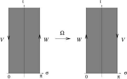
Figure 1: Orientation reversal of the open string worldsheet

Suppose that the left and the right boundary carry Chan-Paton spaces $V$ and $W$ respectively. (See the left part of Figure 1.) If we quantize the open string in such a way that the increase in $t$ corresponds to positive time evolution, the space of states include a factor (Chan-Paton factor)

$${\mathcal{H}}^{\rm CP}={\rm Hom}(V,W).$$ (2.8)

Now, if we consider the orientation reversal,

$$\Omega:(t,\sigma)\longmapsto(t,\pi-\sigma),$$

the left and the right boundaries are swapped and they are oppositely oriented compared to the standard convention we have chosen. Then the Chan-Paton factor is

$$\Omega({\mathcal{H}}^{\rm CP})={\rm Hom}(W^{*},V^{*}).$$ (2.9)

A parity operator includes a complex linear isomorphism

$$P:{\rm Hom}(V,W)\longrightarrow{\rm Hom}(W^{*},V^{*}).$$ (2.10)

Up to automorphisms of $V$ and $W$, a natural candidate is the transpose, $P(\phi)=\phi^{t}$, defined by

$$\langle\phi^{t}f,v\rangle=\langle f,\phi(v)\rangle,\qquad\mbox{for $f\in W^{*}$ and $v\in V$}.$$

However, if $V$ and $W$ are graded vector spaces, it appears more natural to use the graded transpose $P(\phi)=\phi^{T}$ defined by

$$\langle\phi^{T}f,v\rangle=(-1)^{|f||\phi|}\langle f,\phi(v)\rangle.$$

Here $|f|=0$ when $f$ is even and $|f|=1$ if $f$ is odd (similarly for $|\phi|$). Namely, a sign appears whenever two “fermionic” objects swap their positions. In what follows, we confirm this guess using the case where the boundary degrees of freedom are complex (or even number of real) fermions.

Suppose that the left and the right boundaries carry real fermions $\xi_{j}$ ($j=1,...,2m$) and $\eta_{a}$ ($a=1,...,2n$) respectively. The kinetic term of these variables is

$$S_{boundary} = \int_{-\infty}^{\infty}{\rm d}t\sum_{a=1}^{2n}{\frac{i}{2}}\eta_{a}{\frac{{\rm d}}{{\rm d}t}}\eta_{a}+\int_{-\infty}^{\infty}{\rm d}t^{\prime}\sum_{j=1}^{2m}{\frac{i}{2}}\xi_{j}{\frac{{\rm d}}{{\rm d}t^{\prime}}}\xi_{j}$$ (2.11)

$$= \int_{-\infty}^{\infty}{\rm d}t\left[\sum_{a=1}^{2n}{\frac{i}{2}}\eta_{a}{\frac{{\rm d}}{{\rm d}t}}\eta_{a}-\sum_{j=1}^{2m}{\frac{i}{2}}\xi_{j}{\frac{{\rm d}}{{\rm d}t}}\xi_{j}\right].$$

In the first line, $t^{\prime}$ is the time coordinate running in the opposite direction of $t$ ($t^{\prime}=-t$). The Chan-Paton factor on the right (resp. left) boundary is a graded irreducible representation $M_{\eta}$ (resp. $M_{\xi}$) of the Clifford algebra $\{\eta_{a},\eta_{b}\}=\delta_{a,b}$ (resp. $\{\xi_{i},\xi_{j}\}=\delta_{i,j}$) which is unique up to isomorphism. If we quantize the open string in the usual way, where $t$ is the time, the Chan-Paton factor ${\rm Hom}(M_{\xi},M_{\eta})$ must be a graded irreducible representation of the following anti-commutation relations:

$$\{\hat{\eta}_{a},\hat{\eta}_{b}\}=\delta_{a,b},\quad\{\hat{\xi}_{i},\hat{\xi}_{j}\}=-\delta_{i,j},\quad\{\hat{\eta}_{a},\hat{\xi}_{j}\}=0.$$ (2.12)

It is indeed represented on ${\rm Hom}(M_{\xi},M_{\eta})$ by

$$\hat{\eta}_{a}\phi:=\eta_{a}\circ\phi,\qquad\hat{\xi}_{i}\phi:=(-1)^{\phi}\phi\circ\xi_{i}.$$ (2.13)

Note the unusual sign of the $\hat{\xi}$ anticommutators in (2.12): it comes from the unusual sign of the $\xi$-kinetic term in (2.11). The sign factor $(-1)^{\phi}$ in (2.13) is required to produce this sign as well as to satisfy the relation $\{\hat{\eta}_{a},\hat{\xi}_{j}\}=0$.

Let us operate the worldsheet orientation reversal $\Omega$ that swaps the two boundary lines. The Chan-Paton factor is then ${\rm Hom}(M_{\eta}^{*},M_{\xi}^{*})$ since now $\eta_{a}$ is on the left boundary and $\xi_{i}$ on the right, both with the unconventional orientation. The kinetic term remains the same as (2.11) and they must still obey the anticommutaion relations (2.12), which must be represented in ${\rm Hom}(M_{\eta}^{*},M_{\xi}^{*})$. The unique choice (up to isomorphism) is

$$\hat{\eta}_{a}\phi^{*}:=(-1)^{\phi^{*}}\phi^{*}\circ\eta_{a}^{T},\qquad\hat{\xi}_{i}\phi^{*}:=\xi_{i}^{T}\circ\phi^{*}.$$ (2.14)

Here $(-)^{T}$ is the graded transpose, which is needed to obtain the correct sign for the anticommutation relation. Since we simply move $\eta$ from right to left and $\xi$ from left to right, the parity operator

$$P:{\rm Hom}(M_{\xi},M_{\eta})\longrightarrow{\rm Hom}(M_{\eta}^{*},M_{\xi}^{*})$$

must obey

$$P^{-1}\hat{\eta}_{a}P=\hat{\eta}_{a},\quad P^{-1}\hat{\xi}_{i}P=\hat{\xi}_{i}.$$

Namely, $P$ must commute with $\hat{\eta}$ and $\hat{\xi}$. The graded transpose

$$P(\phi)=\phi^{T}$$ (2.15)

satisfies this condition, and it is unique up to scalar multiplication.

2.3 The case of Landau-Ginzburg models

We now consider the parity operation for open strings in Landau-Ginzburg model. A B-type D-brane in the Landau-Ginzburg model is specified by a matrix factorization of the superpotential $W(x^{1},...,x^{n})$,

$$Q(x)=\left(\begin{array}[]{cc}0&f(x)\\ g(x)&0\end{array}\right),\quad Q(x)^{2}=W(x){\bf 1}_{2r}.$$

It enters into the super-Wilson line factor $P\exp\left(-i\int_{\partial\Sigma}{\mathcal{A}}_{t}{\rm d}t\right)$ for the tachyon configuration ${\bf T}=Q+Q^{{\dagger}}$ of the space-filling brane-antibrane system [12]. To be explicit, it is [28, 29, 30]

$${\mathcal{A}}_{t}={\frac{1}{2}}\{Q(x),Q(x)^{{\dagger}}\}+{\frac{1}{2}}\sum_{i=1}^{n}\psi_{i}{\frac{\partial}{\partial x_{i}}}Q(x)+{\frac{1}{2}}\sum_{i=1}^{n}{\frac{\partial}{\partial\overline{x}_{i}}}Q(x)^{{\dagger}}\overline{\psi}_{i}$$

where $\psi_{i}$ are the superpartners of the boundary values of $x_{i}$. Provided $Q(x)^{2}=W(x){\bf 1}$ is satisfied, its supersymmetry variation is given by

$$\delta{\mathcal{A}}_{t}\,=\,-{\rm Re}\left(\,\sum_{i=1}^{n}\overline{\epsilon}\psi_{i}{\frac{\partial}{\partial x_{i}}}W\,\right)-i{\mathcal{D}}_{t}\Bigl{(}\overline{\epsilon}Q+\epsilon Q^{{\dagger}}\Bigr{)}+i\Bigl{(}\dot{\overline{\epsilon}}Q+\dot{\epsilon}Q^{{\dagger}}\Bigr{)},$$ (2.16)

where ${\mathcal{D}}_{t}X=\dot{X}+i[{\mathcal{A}}_{t},X]$. The first term cancels the supersymmetry variation of the bulk action (the Warner term). The second term is a total derivative when inserted in the path-ordered exponentials. The last term shows that $Q$ and $Q^{{\dagger}}$ provides the boundary contribution to the supercharges.

One important point is that $Q$ and $Q^{{\dagger}}$ are secretly fermionic — a sign must appear when a fermionic field $\psi_{i},\overline{\psi}_{i}$ passes through them. We must keep track of such signs when we find out the parity action on matrix factorizations. Although it is possible to do so, we take another route: we consider matrix factorizations that can be realized using boundary fermions where the sign and the statistics are completely under control. For this purpose, it is enough to consider one-by-one factorizations where the super-Wilson-line factor is produced by the path-integral over a single complex boundary fermion $\eta,\overline{\eta}$ with the action (see e.g. [31])

$$S_{\it right}=\int_{-\infty}^{\infty}{\rm d}t\left[i\overline{\eta}{\frac{{\rm d}}{{\rm d}t}}\eta-{\frac{1}{2}}|g(x)|^{2}-{\frac{1}{2}}|f(x)|^{2}-{\rm Re}\Bigl{(}\overline{\eta}\psi^{i}\partial_{i}g(x)+\eta\psi^{i}\partial_{i}f(x)\Bigr{)}\right]_{\sigma=\pi},$$ (2.17)

and supersymmetry variation

$$\delta\eta=-\epsilon\overline{f(x)}-\overline{\epsilon}g(x),\qquad\delta\overline{\eta}=-\overline{\epsilon}f(x)-\epsilon\overline{g(x)}.$$ (2.18)

The subscript “right” emphasizes that it applies to the brane at the right boundary of the string which is oriented in the same direction as the time $t$. On the left boundary, which is oriented oppositely to $t$, the action and the variation are given by

$$S_{\it left}=\int_{-\infty}^{\infty}{\rm d}t\left[-i\overline{\xi}{\frac{{\rm d}}{{\rm d}t}}\xi-{\frac{1}{2}}|\tilde{g}(x)|^{2}-{\frac{1}{2}}|\tilde{f}(x)|^{2}+{\rm Re}\Bigl{(}\overline{\xi}\psi^{i}\partial_{i}\tilde{g}(x)+\xi\psi^{i}\partial_{i}\tilde{f}(x)\Bigr{)}\right]_{\sigma=0},$$ (2.19)

$$\delta\xi=\epsilon\overline{\tilde{f}(x)}-\overline{\epsilon}\tilde{g}(x),\qquad\delta\overline{\xi}=-\overline{\epsilon}\tilde{f}(x)+\epsilon\overline{\tilde{g}(x)},$$ (2.20)

where $\xi,\overline{\xi}$ are a complex fermion, and $(\tilde{f},\tilde{g})$ is another factorization of $W$. With these two boundary terms, the boundary part of the B-type supersymmetry charge is given by

$$Q_{B}=\Bigl{[}f(x)\eta+g(x)\overline{\eta}\Bigr{]}_{\sigma=\pi}-\Bigl{[}\tilde{f}(x)\xi+\tilde{g}(x)\overline{\xi}\Bigr{]}_{\sigma=0}.$$ (2.21)

In particular, using (2.13), we find that this acts on the CP factor ${\rm Hom}(M_{\xi},M_{\eta})$ by

$$Q_{B}\phi=Q\circ\phi-(-1)^{\phi}\phi\circ\tilde{Q}.$$

Now, let us perform the parity $\tau\Omega$. Then the left and the right boundary lines are swapped, and $(f,g)$ and $(\tilde{f},\tilde{g})$ are replaced by $(\tau^{*}f,\tau^{*}g)$ and $(\tau^{*}\tilde{f},\tau^{*}\tilde{g})$. As a consequence, the boundary part of the B-type supercharge is now

$$Q_{B}=\Bigl{[}f(\tau x)\eta+g(\tau x)\overline{\eta}\Bigr{]}_{\sigma=0}-\Bigl{[}\tilde{f}(\tau x)\xi+\tilde{g}(\tau x)\overline{\xi}\Bigr{]}_{\sigma=\pi}$$ (2.22)

Using (2.14), we see that it acts on the Chan-Paton factor ${\rm Hom}(M^{*}_{\eta},M^{*}_{\xi})$ as

$$Q_{B}\phi^{*}=-\tau^{*}\tilde{Q}^{T}\circ\phi^{*}+(-1)^{\phi^{*}}\phi^{*}\circ\tau^{*}Q^{T},$$ (2.23)

where $(-)^{T}$ is the graded transpose. We see that the matrix factorization on the right and the left boundaries are now $-\tau^{*}\tilde{Q}^{T}$ and $-\tau^{*}Q^{T}$.

Let us summarize what we found: Under the simple orientation reversal of the worldsheet, a matrix factorization transforms as

$$Q(x)\longrightarrow-Q(\tau x)^{T},$$ (2.24)

while open string wavefunctions transform as

$$\phi(x)\longmapsto\phi(\tau x)^{T}.$$ (2.25)

In these expressions, $(-)^{T}$ stands for the graded transpose.

2.4 Dual and transpose for graded vector spaces

Since the graded transpose plays an important role, we record below a few basic notions and conventions regarding ${\mathbb{Z}}_{2}$ graded linear algebra. In LG models, it is more convenient to regard the Chan-Paton spaces as (free) modules over the ring ${\mathbb{C}}[x_{1},...,x_{n}]$, rather than complex vector spaces. But we describe everything in the category of complex vector spaces because generalization to modules over the ring is straightforward.

So Let $M$ be a ${\mathbb{Z}}_{2}$ graded (finite-dimensional, complex) vector space with grading operator $\sigma$ which acts as $1$ on even elements and $-1$ on odd elements. The dual vector space $M^{*}={\rm Hom}(M,{\mathbb{C}})$ is naturally graded by $\langle\sigma^{*}f,e\rangle=\langle f,\sigma e\rangle$. Here, we use $\langle\cdot,\cdot\rangle$ to denote the natural pairing $M^{*}\times M\to{\mathbb{C}}$. It is worthwhile emphasizing that despite appearances, this pairing is neither symmetric nor anti-symmetric in any sense. In fact, there is no preference between thinking of the pairing as a map $M^{*}\times M\to{\mathbb{C}}$ or as a map $M\times M^{*}\to{\mathbb{C}}$.

Let us now consider a linear map $A:M_{1}\to M_{2}$ between graded vector spaces $(M_{1},\sigma_{1})$ and $(M_{2},\sigma_{2})$. If $A$ is even (resp. odd), we denote $|A|=0$ (resp. $|A|=1$) modulo 2. We define the (graded) transpose of $A$ as a linear map $A^{T}:M_{2}^{*}\to M_{1}^{*}$ by setting

$$\langle A^{T}f_{2},e_{1}\rangle=(-1)^{|A||f_{2}|}\langle f_{2},Ae_{1}\rangle,$$ (2.26)

if $A$ is even or odd. If $A$ is a linear isomorphism $A^{T}$ is also an isomorphism. The transpose of the inverse and the inverse of the transpose are related by

$$(A^{-1})^{T}=(-1)^{|A|}(A^{T})^{-1}.$$

If $A$ is even, they are the same and we sometimes use the shorthand notation $A^{-T}=(A^{-1})^{T}=(A^{T})^{-1}$.

We wish to emphasize that the definition (2.26) in fact constitutes a choice, and we could have equally well defined

$$\langle{}^{T}\!\!Af_{2},e_{1}\rangle=(-1)^{|A||e_{1}|}\langle f_{2},Ae_{1}\rangle$$ (2.27)

The latter choice is in fact the natural one if we prefer to pair a vector space and its dual in the opposite order. Of course, ${}^{T}\!\!A=(-1)^{|A|}A^{T}$, and one can check that none of our results depend on the choice. Having said that, we will fix the graded transpose defined by (2.26). Let us describe some of its properties.

Matrix representation  Let us choose basis of $M_{1}$ and $M_{2}$ such that even elements come first and odd elements follow them, and suppose that $A$ is expressed with respect to this basis as a matrix

$$A=\left(\begin{array}[]{cc}a&b\\ c&d\\ \end{array}\right)$$ (2.28)

where $a$ maps even to even, $b$ maps odd to even, etc. Then, the matrix representation of the graded transpose of $A$ with respect to the dual basis is

$$A^{T}=\left(\begin{array}[]{cc}a^{T}&-c^{T}\\ b^{T}&d^{T}\end{array}\right),$$ (2.29)

where $a^{T}$, $b^{T}$, $c^{T}$, $d^{T}$ are the transpose matrices of $a$, $b$, $c$, $d$.

Change of grading  Graded transpose of course depends on the gradings $\sigma_{1}$ and $\sigma_{2}$. Let us denote by $A^{T_{\sigma_{1},\sigma_{2}}}$ when we want to show the grading. Then, for change of grading, the graded transpose changes as follows

$$A^{T_{\sigma_{1},-\sigma_{2}}}=-\sigma_{1}^{T}A^{T_{\sigma_{1},\sigma_{2}}},\qquad A^{T_{-\sigma_{1},\sigma_{2}}}=A^{T_{\sigma_{1},\sigma_{2}}}\sigma_{2}^{T},\quad A^{T_{-\sigma_{1},-\sigma_{2}}}=\sigma_{1}^{T}A^{T_{\sigma_{1},\sigma_{2}}}\sigma_{2}^{T}.$$ (2.30)

Note that $\sigma$ is always even and thus its transpose $\sigma^{T}$ does not depend on the grading used.

Composition  Graded transpose obeys an interesting property under composition. Let $B:M_{1}\to M_{2}$ and $A:M_{2}\to M_{3}$ be linear maps. Suppose each of them is even or odd, so that $|A|$ and $|B|$ makes sense. Then we have

$$(AB)^{T}=(-1)^{|A||B|}B^{T}A^{T}.$$ (2.31)

Since this is important, let us record the proof here:

$$\begin{split}\langle(AB)^{T}f_{3},e_{1}\rangle_{1}&=(-1)^{|AB||f_{3}|}\langle f_{3},ABe_{1}\rangle_{3}\\ &=(-1)^{|AB||f_{3}|+|A||f_{3}|}\langle A^{T}f_{3},Be_{1}\rangle_{2}\\ &=(-1)^{|AB||f_{3}|+|A||f_{3}|+|B||A^{T}f_{3}|}\langle B^{T}A^{T}f_{3},e_{1}\rangle_{1}.\end{split}$$ (2.32)

Using $|AB|=|A|+|B|$, $|A^{T}f_{3}|=|A^{T}|+|f_{3}|=|A|+|f_{3}|$, we find that the sign that appears on the right hand side is $(-1)^{|B||A|}$. This shows (2.31).

Tensor product  It is also important to study and fix our convention on tensor products. Let $(M_{1},\sigma_{1})$ and $(M_{2},\sigma_{2})$ be graded vector spaces. The tensor product $M_{1}\otimes M_{2}$ has a natural grading $\sigma_{12}=\sigma_{1}\otimes\sigma_{2}$. Its dual is identified with $M_{1}^{*}\otimes M_{2}^{*}$ whose dual is in turn identified with $M_{1}\otimes M_{2}$, so that

$$\langle a_{1}\otimes a_{2},b_{1}\otimes b_{2}\rangle_{12}=(-1)^{|a_{2}||b_{1}|}\langle a_{1},b_{1}\rangle_{1}\langle a_{2},b_{2}\rangle_{2}$$ (2.33)

holds for $a_{1},b_{1}\in M_{1}\oplus M_{1}^{*}$ and $a_{2},b_{2}\in M_{2}\oplus M_{2}^{*}$. For linear maps $A_{1}:M_{1}\to N_{1}$ and $A_{2}:M_{2}\to N_{2}$ of graded vector spaces, their tensor product map is defined by

$$(A_{1}\otimes A_{2})(a_{1}\otimes a_{2})=(-1)^{|A_{2}||a_{1}|}(A_{1}a_{1})\otimes(A_{2}a_{2}).$$

One can show that the transpose map $N_{1}^{*}\otimes N_{2}^{*}\to M_{1}^{*}\otimes M_{2}^{*}$ of this is given by

$$(A_{1}\otimes A_{2})^{T}=A_{1}^{T}\otimes A_{2}^{T}.$$ (2.34)

Double dual, double transpose  For a graded vector space $M$, the dual of $M^{*}$ is isomorphic to $M$. An isomorphism $\iota:M\to M^{**}$ (which we call the canonical isomorphism) is defined by the property

$$\langle\iota(v),f\rangle=(-1)^{|v||f|}\langle f,v\rangle.$$ (2.35)

It of course depend on the grading $\sigma$, and we sometimes write $\iota_{M,\sigma}$ or $\iota_{\sigma}$. Definition (2.35) comes with a few oddities (compared to, let’s say, $\langle\tilde{\iota}(v),f\rangle=\langle f,v\rangle$). If we choose a basis of $M$ where even elements come first, with respect to it and its dual-dual basis, $\iota$ is represented as

$$\iota=\left(\begin{array}[]{cc}1&0\\ 0&-1\end{array}\right).$$ (2.36)

If $A:M_{1}\to M_{2}$ is a linear map of graded vector spaces, the map $A^{TT}:M_{1}^{**}\to M_{2}^{**}$ is related to $A$ by

$$A^{TT}=\iota_{2}A\iota_{1}^{-1}.$$ (2.37)

If we flip the grading, the canonical isomorphism changes by sign

$$\iota_{-\sigma}=-\iota_{\sigma}.$$ (2.38)

3 Parities as Functors

As is well-known [6, 7], in a theory of oriented strings the collection of all D-branes forms a category ${\mathcal{C}}$ (to be precise, in a slightly generalized sense). Objects of ${\mathcal{C}}$ are D-branes, $B_{i}$, the space of morphisms between two objects, ${\rm Hom}(B_{1},B_{2})$, is the space of states of the open string stretched from the brane $B_{1}$ to the brane $B_{2}$. The composition of morphisms dictates the process of two strings joining into one.

In this language, a parity operation can be regarded as an anti-involution of that category. By definition, it is a contravariant functor

$${\mathcal{P}}:{\mathcal{C}}\to{\mathcal{C}},$$ (3.1)

whose square is isomorphic to the identity,

$${\cal P}\circ{\cal P}\cong{{\rm id}}_{\mathcal{C}}.$$ (3.2)

Namely, to each brane $B$ a brane ${\mathcal{P}}(B)$ is assigned as its parity image. For each pair of branes $(B_{1},B_{2})$ there is a linear isomorphism

$${\mathcal{P}}:\phi\in{\rm Hom}(B_{1},B_{2})\longmapsto{\mathcal{P}}(\phi)\in{\rm Hom}({\mathcal{P}}(B_{2}),{\mathcal{P}}(B_{1})),$$

mapping states of the open string from $B_{1}$ to $B_{2}$ to states of the open string from ${\mathcal{P}}(B_{2})$ to ${\mathcal{P}}(B_{1})$, in a way compatible with the joining process. Furthermore, if the parity is operated twice on a brane the result is isomorphic to the original brane, ${\mathcal{P}}({\mathcal{P}}(B))\cong B$, in a way consistent with everything.

In what follows, we define such parity functors in the categories of D-branes associated with a LG model. We start with describing the categories themselves. (This is a review.)

3.1 The category of matrix factorizations

As discussed above, the data to specify a B-brane in the LG model is a matrix factorization $Q(x)$ of the superpotential $W(x)$. This can be interpreted as an open string tachyon configuration on a stack of equal numbers of space filling branes and anti-branes. We regard this as a triple

$$(M,\sigma,Q)$$ (3.3)

where $M$ is a free module over the polynomial ring $S={\mathbb{C}}[x_{1},...,x_{n}]$, with ${\mathbb{Z}}_{2}$ grading $\sigma$, and $Q$ is an odd endomorphism of $M$ which squares to $W$ times the identity of $M$. The (truncated off-shell) space of open string states between two branes determined by matrix factorizations $(M_{1},\sigma_{1},Q_{1})$ and $(M_{2},\sigma_{2},Q_{2})$ is the space of homomorphisms of the modules ${\rm Hom}_{S}(M_{1},M_{2})$. The supercharge action is represented by ${\rm d}\phi=Q_{2}\phi-\sigma_{2}\phi\sigma_{1}Q_{1}$. Matrix factorizations of $W$ with $\bigl{(}{\rm Hom}_{S}(M_{1},M_{2}),{\rm d}\bigr{)}$ as morphism spaces form a differential graded category which we denote by $\Scr{M\!F}(W)$. Its homotopy category ${\rm MF}(W)$, obtained by simply restricting morphisms to be ${\rm d}$-cohomology classes, is triangulated [32, 33, 34].

In the case of LG orbifolds, the data for a brane includes an even representation $\rho$ of $\Gamma$ on $M$, satisfying the condition

$$\rho(g)Q(gx)\rho(g)^{-1}=Q(x)\qquad\text{for $g\in\Gamma$}$$ (3.4)

This is of course nothing else but the original orbifold construction of [27], actually with the simplification that all branes, being space filling, are invariant under $\Gamma$. Therefore, we only have an action on the Chan-Paton space $M$ together with the action on closed string variables. Thus, a B-brane in the LG orbifold is specified by the data

$$(M,\sigma,Q,\rho).$$ (3.5)

For a pair branes given by such data, $(M_{1},\sigma_{1},Q_{1},\rho_{1})$ and $(M_{2},\sigma_{2},Q_{2},\rho_{2})$, the space of open strings between them is given by the $\Gamma$-invariant homomorphisms ${\rm Hom}_{S}(M_{1},M_{2})^{\Gamma}$ with respect to the action $g\in\Gamma:\phi\mapsto\rho_{2}(g)g^{*}\phi\rho_{1}(g)^{-1}$. These data form a differential graded category $\Scr{M\!F}_{\Gamma}(W)$ and we denote its homotopy category by ${\rm MF}_{\Gamma}(W)$ which is again triangulated. The group $\Gamma^{*}$ of quantum symmetries acts as the auto-equivalence of these categories by $(M,\sigma,Q,\rho)\mapsto(M,\sigma,Q,g^{*}(\rho))$, where $(g^{*}(\rho))(g)=g^{*}(g)\,\rho(g)$ for $g^{*}\in\Gamma^{*}$, $g\in\Gamma$.

3.2 The parity functors

Let us now define the parity functors on these categories. We first consider the case without orbifold. An example is already found in section 2.3: a matrix factorization $Q(x)$ is sent to $-Q(\tau x)^{T}$ and a morphism $\phi(x)$ is mapped to $\phi(\tau)^{T}$, see Eqn (2.24) and Eqn. (2.25). Thus, we propose to define a functor $\Scr{P}:\Scr{M\!F}(W)\to\Scr{M\!F}(W)$ by

$$\begin{split}(M,\sigma,Q)&\longmapsto(M^{*},\sigma^{T},-\tau^{*}Q^{T}),\\ {\rm Hom}_{S}(M_{1},M_{2})\ni\phi&\longmapsto\tau^{*}\phi^{T}\in{\rm Hom}_{S}(M_{2}^{*},M_{1}^{*}).\end{split}$$ (3.6)

It meets the conditions:
$\bullet$ $\Scr{P}(M,\sigma,Q)$ is a matrix factorization of $W$

$$\begin{split}(-\tau^{*}Q^{T})^{2}&=\tau^{*}Q^{T}\tau^{*}Q^{T}=-(\tau^{*}Q\tau^{*}Q)^{T}=-(\tau^{*}W\cdot{\rm id}_{M})^{T}\\ &=-(-W)\cdot{\rm id}_{M^{*}}=W\cdot{\rm id}_{M^{*}},\end{split}$$ (3.7)

where we have used (2.31) in the second equality and also (2.2) in the fourth.
$\bullet$ It commutes with the supercharge: For $\phi\in{\rm Hom}_{S}(M_{1},M_{2})$ which is either even or odd, $\sigma_{2}\phi\sigma_{1}=(-1)^{|\phi|}\phi$, we have

$$\begin{split}{\rm d}\Scr{P}(\phi)&=(-\tau^{*}Q_{1}^{T})\tau^{*}\phi^{T}-(-1)^{|\phi|}\tau^{*}\phi^{T}(-\tau^{*}Q_{2}^{T})\\ &=-(-1)^{|\phi|}(\tau^{*}\phi\tau^{*}Q_{1})^{T}+(\tau^{*}Q_{2}\tau^{*}\phi)^{T}\\ &=\tau^{*}(Q_{2}\phi-(-1)^{|\phi|}\phi Q_{1})^{T}=\Scr{P}({\rm d}\phi)\end{split}$$ (3.8)

$\bullet$ It is compatible with the composition: For $\phi\in{\rm Hom}_{S}(M_{1},M_{2})$ and $\psi\in{\rm Hom}_{S}(M_{2},M_{3})$, their composition $\psi\phi\in{\rm Hom}_{S}(M_{1},M_{3})$ is mapped to

$$\Scr{P}(\psi\phi)=\tau^{*}(\psi\phi)^{T}=(-1)^{|\psi||\phi|}\tau^{*}\phi^{T}\tau^{*}\psi^{T}=(-1)^{|\psi||\phi|}\Scr{P}(\phi)\Scr{P}(\psi).$$ (3.9)

$\bullet$ The square of $\Scr{P}$ does

$$\begin{split}\Scr{P}^{2}&:(M,\sigma,Q)\longmapsto(M^{**},\sigma^{TT},\tau^{*}(\tau^{*}Q^{T})^{T})=(M^{**},\sigma^{TT},Q^{TT}),\\ \Scr{P}^{2}&:{\rm Hom}_{S}(M_{1},M_{2})\ni\phi\longmapsto\phi^{TT}\in{\rm Hom}_{S}(M_{1}^{**},M_{2}^{**}).\end{split}$$ (3.10)

Using the relation (2.37), we see that the canonical isomorphism $\iota:M\to M^{**}$ provides an isomorphism of $\Scr{P}^{2}$ to the identity,

$$\iota:\Scr{P}\stackrel{{\scriptstyle\cong}}{{\longrightarrow}}{\rm id}_{\Scr{M\!F}(W)}.$$

Thus, $\Scr{P}$ is an anti-involution of the differential graded category $\Scr{M\!F}(W)$. As a consequence, it descends to a functor of the homotopy category ${\rm MF}(W)$. Namely, $\Scr{P}$ defines a map of ${\rm d}$-cohomology classes by the property (3.8).

One may obtain other parity functors by composing the above $\Scr{P}$ with some other auto-equivalence of $\Scr{M\!F}(W)$. For example, $\Scr{M\!F}(W)$ has antibrane functor $\Scr{A}$ that sends $(M,\sigma,Q)$ to $(M,-\sigma,Q)$. Let us examine the composition $\Scr{A}\!\Scr{P}:=\Scr{A}\circ\Scr{P}$

$$\Scr{A}\!\Scr{P}:(M,\sigma,Q)\longmapsto(M^{*},-\sigma^{T},-\tau^{*}Q^{T}).$$

The transpose “$T$” is with respect to the grading $\sigma$. It is easy to see that it is a matrix factorization of $W$, and that ${\rm d}\Scr{A}\!\Scr{P}(\phi)=\Scr{A}\!\Scr{P}({\rm d}\phi)$ for any open string state $\phi$. The square of $\Scr{A}\!\Scr{P}$ does

$$\begin{split}(\Scr{A}\!\Scr{P})^{2}&:(M,\sigma,Q)\longmapsto(M^{**},\sigma^{TT},-Q^{TT}),\\ (\Scr{A}\!\Scr{P})^{2}&:{\rm Hom}_{S}(M_{1},M_{2})\ni\phi\longmapsto(\sigma_{2}\phi\sigma_{1})^{TT}\in{\rm Hom}_{S}(M_{1}^{**},M_{2}^{**})\end{split}$$ (3.11)

where we have used (2.30). We see that $\iota\circ\sigma:M\to M^{**}$ provides an isomorphism of $(\Scr{A}\!\Scr{P})^{2}$ to the identity.

3.3 LG orbifolds

Let us next consider the orbifold of the LG model by a finite abelian group $\Gamma$ that preserves the superpotential, $g^{*}W=W$ for all $g\in\Gamma$. We suppose that an abelian extension of ${\mathbb{Z}}_{2}$ by $\Gamma$

$$1\longrightarrow\Gamma\longrightarrow\widehat{\Gamma}\longrightarrow{\mathbb{Z}}_{2}\longrightarrow 1,$$

also acts on the variables, so that elements $\tau\in\widehat{\Gamma}$ outside of $\Gamma$ flip the sign of $W$, $\tau^{*}W=-W$. One can consider a parity symmetry associated with the group $\widehat{\Gamma}/\Gamma$.

We would like to find parity actions on B-branes and open string states. The requirement is as before — we seek anti-involutions of the categories $\Scr{M\!F}_{\Gamma}(W)$ and ${\rm MF}_{\Gamma}(W)$. Let us choose any odd element $\tau\in\widehat{\Gamma}\setminus\Gamma$, and consider

$$\Scr{P}(\tau):(M,\sigma,Q,\rho)\longmapsto(M^{*},\sigma^{T},-\tau^{*}Q^{T},\rho^{-T}).$$ (3.12)

It is easy to see that $\phi\mapsto\tau^{*}\phi^{T}$ maps $\Gamma$-invariants to $\Gamma$-invariants;

$$\Scr{P}(\tau):\phi\in{\rm Hom}_{S}(M_{1},M_{2})^{\Gamma}\longmapsto\tau^{*}\phi^{T}\in{\rm Hom}_{S}(M_{2}^{*},M_{1}^{*})^{\Gamma}.$$ (3.13)

The square of $\Scr{P}(\tau)$ is isomorphic to the identity by the canonical isomorphism $\iota:M\to M^{**}$. It commutes with the supercharge and thus the functor descends to the homotopy category. For any $g\in\Gamma$, $\Scr{P}(\tau g)$ is isomorphic to $\Scr{P}(\tau)$ by $\rho(g):M\to M$. However, it may appear unpleasant that we need to make a choice of $\tau\in\widehat{\Gamma}\setminus\Gamma$. This worry actually disappears when we appropriately define the D-brane category in the orientifold. See Section 4.2.

One may dress the action on $\rho$ by a character $\chi:\Gamma\longrightarrow{\mathbb{C}}^{\times}$,

$$\Scr{P}_{\chi}(\tau):(M,\sigma,Q,\rho)\longmapsto(M^{*},\sigma^{T},-\tau^{*}Q^{T},\chi\rho^{-T}).$$ (3.14)

We also have $\Scr{A}\!\Scr{P}_{\chi}(\tau)=\Scr{A}\circ\Scr{P}_{\chi}(\tau)$.

4 Category of D-branes in Orientifolds

So far, we have discussed parity as an anti-involution of the category of D-branes. In constructing an orientifold background in string theory, we intend to promote parity from a global symmetry to a gauge symmetry. In particular, we want to include into the background a configuration of D-branes that is invariant by the parity, and classify open string states with specific transformation properties under the parity.

This motivates us to consider a new category of D-branes, whose objects are invariant brane configurations or simply invariant branes. Let ${\mathcal{C}}$ be a category of D-branes with a parity functor ${\mathcal{P}}$. An invariant brane is a brane $B$ with an isomorphism

$$U:{\mathcal{P}}(B)\longrightarrow B.$$ (4.1)

For a pair of invariant branes, $(B_{1},U_{1})$ and $(B_{2},U_{2})$, there is a linear map

$$P:{\rm Hom}(B_{1},B_{2})\stackrel{{\scriptstyle{\mathcal{P}}}}{{\longrightarrow}}{\rm Hom}({\mathcal{P}}(B_{2}),{\mathcal{P}}(B_{1}))\stackrel{{\scriptstyle U_{1}\cdot(?)\cdot U_{2}^{-1}}}{{\longrightarrow}}{\rm Hom}(B_{2},B_{1}).$$ (4.2)

We require that this linear map be an involution

$$P\circ P={{\rm id}}_{{\rm Hom}(B_{1},B_{2})}.$$ (4.3)

In order to impose orientifold projection, we want $P^{2}$ to be literally the identity operator of the space of states ${\rm Hom}(B_{1},B_{2})$. (It is not enough for ${\cal P}^{2}$ to be isomorphic to the identify.) This is a rather strong condition on the collection of invariant objects $(B,U)$. It is possible that, for each functor ${\mathcal{P}}$, there are several categories consisting of invariant branes that are mutually compatible in the sense that (4.3) holds for any pair. As for the morphisms in the new categories, the best choice is to keep all morphisms from before the orientifold, as we will discuss below.

The purpose of this section is to show that one can indeed define such categories and to classify them, in Landau-Ginzburg models and their orbifolds.

4.1 The categories $\Scr{M\!F}_{{\Scr{P}}}^{\,\epsilon}(W)$ and ${\rm MF}_{{\Scr{P}}}^{\,\epsilon}(W)$

We start with the unorbifolded Landau-Ginzburg model with an involution $x\mapsto\tau x$ such that $W(\tau x)=-W(x)$. As the parity functor, let us first take ${\mathcal{P}}=\Scr{P}$ defined in (3.6). An invariant brane is a quadruple $(M,\sigma,Q,U)$ where $(M,\sigma,Q)$ is a matrix factorization of $W(x)$ and $U$ is a linear isomorphism

$$U:M^{*}\longrightarrow M,$$ (4.4)

such that

$$\begin{split}&U\sigma^{T}U^{-1}=\sigma,\\[5.69046pt] &U(-\tau^{*}Q^{T})U^{-1}=Q.\end{split}$$ (4.5)

For a pair of such branes, $(M_{1},\sigma_{1},Q_{1},U_{1})$ and $(M_{2},\sigma_{2},Q_{2},U_{2})$, the parity transformation of the open string states is defined according to (4.2):

$$P:\phi\in{\rm Hom}_{S}(M_{1},M_{2})\longmapsto U_{1}\tau^{*}\phi^{T}U_{2}^{-1}\in{\rm Hom}_{S}(M_{2},M_{1}).$$ (4.6)

The square of $P$ is given by

$$P^{2}(\phi) = U_{2}\tau^{*}(U_{1}\tau^{*}\phi^{T}U_{2}^{-1})^{T}U_{1}^{-1}=U_{2}U_{2}^{-T}\phi^{TT}U_{1}^{T}U_{1}^{-1}$$

$$= U_{2}U_{2}^{-T}\iota_{2}\phi\iota_{1}^{-1}U_{1}^{T}U_{1}^{-1},$$

where $\phi^{TT}=\iota_{2}\phi\iota_{1}^{-1}$ is used in the last step (see (2.37)). We require that the right hand side equals $\phi$ itself for any $\phi\in{\rm Hom}_{S}(M_{1},M_{2})$. By Schur’s Lemma, this means that $U_{2}U_{2}^{-T}\iota_{2}$ and $U_{1}U_{1}^{-T}\iota_{1}$ are the same matrix which is proportional to the identity. Thus, we find that, in a category of mutually compatible branes, we have

$$UU^{-T}\iota=\epsilon\cdot{\rm id}_{M}$$ (4.7)

where $\epsilon$ is a constant that is independent of the brane in that category. Using $U=\epsilon\iota^{-1}U^{T}$ twice and employing the relation $\iota^{-1}U^{TT}\iota^{-T}=U$, we find that

$$\epsilon^{2}=1.$$

Thus, we obtain a category parametrized by a sign $\epsilon$, which we denote by $\Scr{M\!F}_{\!\Scr{P}}^{\,\epsilon}(W)$. As for the morphisms, we decide to keep everything. Namely the space of morphisms from $(M_{1},\sigma_{1},Q_{1},U_{1})$ to $(M_{2},\sigma_{2},Q_{2},U_{2})$ is still ${\rm Hom}_{S}(M_{1},M_{2})$. (This point will be discussed further in Section 4.4 below.) Then $\Scr{M\!F}_{\!\Scr{P}}^{\,\epsilon}(W)$ is a differential graded category. One can show that the linear map $P:{\rm Hom}_{S}(M_{1},M_{2})\to{\rm Hom}_{S}(M_{2},M_{1})$ in (4.6) commutes with the supercharge, since we have

$$\forall\psi\in{\rm Hom}_{S}(M_{2}^{*},M_{1}^{*}),\qquad{\rm d}(U_{1}\psi U_{2}^{-1})=U_{1}({\rm d}\psi)U_{2}^{-1}$$

provided the condition (4.5) holds for both $(M_{1},\sigma_{1},Q_{1},U_{1})$ to $(M_{2},\sigma_{2},Q_{2},U_{2})$. This means that we also have the homotopy category ${\rm MF}_{\Scr{P}}^{\,\epsilon}(W)$ consisting of invariant branes with the constant $\epsilon$.

Similarly, we can construct the new categories based on the parity functor ${\mathcal{P}}=\Scr{A}\!\Scr{P}$.

4.2 LG orbifolds

In orientifolding a LG orbifold, we consider the parity functor’s ${\mathcal{P}}=\Scr{P}_{\chi}(\tau)$’s introduced in (3.14). An invariant brane is a quintuple $(M,\sigma,Q,\rho,U)$ where $(M,\sigma,Q,\rho)$ is an object of $\Scr{M\!F}_{\Gamma}(W)$ and $U$ assigns to each odd element $\tau\in\widehat{\Gamma}$ an isomorphism

$$U(\tau):M^{*}\to M$$ (4.8)

such that

$$\begin{split}&U(\tau)\sigma^{T}U(\tau)^{-1}=\sigma,\\[2.84544pt] &U(\tau)(-\tau^{*}Q^{T})U(\tau)^{-1}=Q,\\[2.84544pt] &U(\tau)(\chi\rho^{-T})U(\tau)^{-1}=\rho.\end{split}$$ (4.9)

Without loss of generality, one can assume

$$U(g\tau)\rho(g)^{T}=\chi(g)U(\tau),\qquad\forall g\in\Gamma,\quad\forall\tau\in\widehat{\Gamma}\setminus\Gamma.$$ (4.10)

In fact, suppose we have $U(\tau)$’s obeying only (4.9) but not necessarily (4.10). Then, pick and fix any $\tau_{0}\in\widehat{\Gamma}\setminus\Gamma$ and modify $U(\tau)$ by $\tilde{U}(\tau)=\rho(\tau\tau_{0}^{-1})U(\tau_{0})$. Then (4.10) as well as all the conditions in (4.9) are satisfied for $\tilde{U}(\tau)$. In what follows, we always assume the relation (4.10).

For two such invariant branes $(M_{i},\sigma_{i},Q_{i},\rho_{i},U_{i})$, $i=1,2$, the parity transformation ${\rm Hom}_{S}(M_{1},M_{2})^{\Gamma}\to{\rm Hom}_{S}(M_{2},M_{1})^{\Gamma}$ is defined as

$$P_{\chi}(\phi)=U_{1}(\tau)\tau^{*}\phi^{T}U_{2}(\tau)^{-1}.$$ (4.11)

Because of the relation (4.10) this is independent of the choice of $\tau$. At this stage, we require that $P_{\chi}$ be involutive on the equivariant category. As before, the content of the requirement is found by computing $P_{\chi}^{2}$, and yields the condition that

$$U(\tau)U(\tau)^{-T}\iota\rho(\tau^{2})^{-1}=c(\tau)\cdot{\rm id}_{M}$$ (4.12)

hold for any brane $(M,\sigma,Q,\rho,U)$, where $c(\tau)$ is a phase that is independent of the brane in a mutually compatible class. Using $U(\tau)=c(\tau)\rho(\tau^{2})\iota^{-1}U(\tau)^{T}$ twice, and with the help of the last condition in (4.9), we find the relation

$$c(\tau)^{2}\chi(\tau^{2})=1.$$ (4.13)

Combining (4.12) and (4.10) and again with the help of the last condition in (4.9) we find

$$c(g\tau)=\chi(g)^{-1}c(\tau).$$ (4.14)

This together with $c(\tau)^{2}\chi(\tau^{2})=1$ means that the function $c(\tau)$ is, up to a sign, again uniquely determined by the choice of parity.

Summarizing, we have defined the D-brane category $\Scr{M\!F}_{\!\Scr{P}_{\chi}}^{\pm c}(W)$ which is differential graded and its homotopy category ${\rm MF}_{\!\Scr{P}_{\chi}}^{\pm c}(W)$.

4.3 Invariant branes from irreducible ones

We have seen that in both LG model and LG orbifold, the possible D-brane categories for a given parity are classified by a sign: $\epsilon=\pm 1$ in (4.7) for the model without orbifold, and for orbifold $c(\tau)$ in (4.12) admits only two possibilities: say, $c(\tau)=c_{0}(\tau)$ or $c(\tau)=-c_{0}(\tau)$. These signs are actually the standard sign ambiguity for the orientifold projection in the open string sector.

To see this, we study irreducible branes in the orbifold theory and stacks of them that can or cannot be members of one of these categories. Let $B=(M,\sigma,Q,\rho)$ be an irreducible matrix factorization. By definition, “irreducible” means that there is no subspace of $M$ that is invariant under both $\rho$ and $Q$. Suppose it is also invariant under the parities ${\mathcal{P}}_{\chi}(\tau)$ for $\tau\in\widehat{\Gamma}$. Namely, there is an $U(\tau):M^{*}\to M$ that obey (4.9). We deduce

$$\begin{split}Q(x)&=U(\tau)U(\tau)^{-T}\iota Q(\tau^{2}x)\iota^{-1}U(\tau)^{T}U(\tau)^{-1}\\ &=U(\tau)U(\tau)^{-T}\iota\rho(\tau^{2})^{-1}Q(x)\rho({\tau^{2}})\iota^{-1}U(\tau)^{T}U(\tau)^{-1}\end{split}$$ (4.15)

From irreducibility, it follows

$$U(\tau)U(\tau)^{-T}\iota=\alpha(\tau)\rho(\tau^{2})$$ (4.16)

where $\alpha(\tau)$ is a phase. Thence

$$\alpha(\tau)^{2}\chi(\tau)^{2}=1.$$

We also have $\alpha(g\tau)=\chi(g)^{-1}\alpha(\tau)$. Therefore $\alpha(\tau)=\pm c_{0}(\tau)=:\epsilon^{\rm int}c_{0}(\tau)$, and the “internal” sign $\epsilon^{\rm int}=\pm 1$ is uniquely associated with $B$. We then choose an “external” Chan-Paton space $V\cong{\mathbb{C}}^{N}$ together with a map $\gamma:V^{*}\to V$ and define

$$\begin{split}\hat{M}&=V\otimes M\\ \hat{Q}&=1\otimes Q\\ \hat{U}(\tau)&=\gamma\otimes U(\tau)\qquad\tau\in\widehat{\Gamma}\setminus\Gamma\\ \hat{\rho}(g)&=1\otimes\rho(g)\qquad g\in\Gamma\end{split}$$ (4.17)

This definition satisfies the condition (4.9), and we find

$$\hat{U}(\tau)\hat{U}(\tau)^{-T}\iota=\gamma\gamma^{-T}\otimes U(\tau)U(\tau)^{-T}\iota=\gamma\gamma^{-T}\otimes\alpha(\tau)\rho(\tau^{2})$$ (4.18)

Therefore, the brane $(\hat{M},\hat{\sigma},\hat{Q},\hat{\rho},\hat{U})$ is a member of the category $\Scr{M\!F}_{\!\Scr{P}_{\chi}}^{c}(W)$ with $c=\epsilon c_{0}$ if

$$\gamma\gamma^{-T}=\epsilon^{\rm ext}=\epsilon^{\rm int}\epsilon.$$

It is this sign, $\epsilon^{\rm ext}$, which decides whether the gauge group on $\hat{Q}$ is of symplectic or orthogonal type. This is as usual: Given an overall choice of orientifold sign $\epsilon$, and the internal sign $\epsilon^{\rm int}$ which one discovers for any given $Q$ by an explicit computation, one can decorate this brane only with a CP space with appropriate $\epsilon^{\rm ext}$.

For completeness, we also consider the case where the irreducible brane $B=(M,\sigma,Q,\rho)$ is not invariant, i.e. there is no $U(\tau):M^{*}\to M$ that obey (4.9) and (4.10). Then we can still form an invariant brane by combining $B$ with its parity image and tensoring with an external Chan-Paton space $V={\mathbb{C}}^{N}$. Namely we define

$$\begin{split}&\hat{M}=(V\otimes M)\,\oplus\,(V^{*}\otimes M^{*}),\\ &\hat{\sigma}=\left(\begin{array}[]{cc}\sigma&0\\ 0&\sigma^{T}\end{array}\right),\\ &\hat{Q}=\left(\begin{array}[]{cc}Q&0\\ 0&-\tau_{0}^{*}Q^{T}\end{array}\right)\\ &\hat{\rho}=\left(\begin{array}[]{cc}\rho&0\\ 0&\chi\rho^{-T}\end{array}\right),\end{split}$$ (4.19)

where $\tau_{0}$ is an arbitrarily chosen odd element of the group $\widehat{\Gamma}$. Then, this is invariant using $\hat{U}(\tau):\hat{M}^{*}\to\hat{M}$ given by

$$\hat{U}(\tau)=\chi(\tau\tau_{0}^{-1})\left(\begin{array}[]{cc}0&\alpha(\tau)\rho(\tau\tau_{0})\iota^{-1}\\ \rho(\tau\tau_{0}^{-1})&0\end{array}\right),$$ (4.20)

where $\alpha$ is some phase. If we choose $\alpha(\tau)=c(\tau)$, this satisfies

$$\hat{U}(\tau)\hat{U}(\tau)^{-T}\hat{\iota}\hat{\rho}(\tau^{2})^{-1}=\left(\begin{array}[]{cc}c(\tau)&0\\ 0&c(\tau)\end{array}\right),$$ (4.23)

$$\hat{U}(g\tau)\hat{\rho}(g)^{T}=\chi(g)\hat{U}(\tau).$$

Thus $\hat{B}=(\hat{M},\hat{\sigma},\hat{Q},\hat{\rho},\hat{U})$ is a member of the category $\Scr{M\!F}_{\!\Scr{P}_{\chi}}^{\,c}(W)$. The gauge group is $U(N)$ in this case.

4.4 Morphisms and gauge algebra

We have seen above that parity acts on the morphism spaces of both $\Scr{M\!F}(W)$ and ${\rm MF}(W)$, and that requiring this action to be involutive leaves the freedom of an overall choice of sign, $\epsilon$, in the action of parity on individual objects. One is then tempted to try to impose parity invariance also on the morphism spaces. But some care is required.

First note that even for invariant objects $B=(M,\sigma,Q,U)$ and $B^{\prime}=(M^{\prime},\sigma^{\prime},Q^{\prime},U^{\prime})$, parity does not send the morphism space ${\rm Hom}_{S}(M,M^{\prime})$ to itself, but to ${\rm Hom}_{S}(M^{\prime},M)$ (where we are using the isomorphisms $U:M^{*}\to M$, $U^{\prime}:M^{\prime*}\to M^{\prime}$). The minimal morphism spaces on which parity acts are, for $B\neq B^{\prime}$,

$$\hat{\rm H}{\rm om}(M,M^{\prime}):={\rm Hom}_{S}(M,M^{\prime})\oplus{\rm Hom}_{S}(M^{\prime},M)\,,$$ (4.24)

which can then indeed be decomposed into even and odd components under parity. For the endomorphisms of an invariant object $B=B^{\prime}$, we can be slightly more economical, and consider the action of parity on

$$\hat{\rm E}{\rm nd}(M):={\rm Hom}_{S}(M,M)$$ (4.25)

Note that $\hat{\rm E}{\rm nd}(M)\neq\hat{\rm H}{\rm om}(M,M)$ according to these definitions.

The peculiarity of parity (as compared with other discrete symmetries) is that it does not define an automorphism of the operator algebra of open strings, but rather an anti-automorphism. Namely, parity reverses the cyclic ordering of operators inserted on the boundary of the worldsheet. See Fig. 2. As a consequence, parity does not impose any selection rule on worldsheet correlators with more than two boundary insertions. (For just two insertions, which defines the topological metric, parity does yield a selection rule.) If these statements come as a surprise, we hasten to emphasize that of course in full string theory, orientifolding does define a projection that is consistent with string interactions. This is a consequence of integrating over the moduli space of Riemann surfaces, and in particular, summing over the ordering of operators on the boundary.

Figure 2: A disk correlator and its parity image. The existence of this symmetry does not (unfortunately) impose any restrictions on the parities of $\phi_{1}$, $\phi_{2}$, $\phi_{3}$. For example, the correlator could be non-zero for $P_{1}=-,P_{2}=+,P_{3}=+$.

Nevertheless, even if the topological field theory does not admit the “orientifold projection”, we can still learn about the effect of this projection in the string background built on the parity of our Landau-Ginzburg model. Consider strings from one brane to itself. In both the ordinary and the orbifolded case, we have shown that $P^{2}(\phi)=\phi$ for $\phi\in{\rm Hom}(M,M)$. We can then decompose

$$\hat{\rm E}{\rm nd}(M)={\rm Hom}(M,M)=\hat{\rm E}{\rm nd}^{+}(M)\oplus\hat{\rm E}{\rm nd}^{-}(M)$$ (4.26)

where

$$P(A)=\pm A\qquad\text{for $A\in\hat{\rm E}{\rm nd}^{\pm}(M)$, respectively.}$$ (4.27)

As we have noted, we cannot consistently compose morphisms in a way that is compatible with this decomposition. This is because a diagram as Fig. 2 for $P(A)=P_{A}A$, $P(B)=P_{B}B$ only implies $P(AB)=(-1)^{|A||B|}P_{A}P_{B}BA$, which is not necessarily related to $AB$. However, the Lie algebra structure inherited from ${\rm Hom}(M,M)$,

$$\{A,B\}=AB-(-1)^{AB}BA$$ (4.28)

is preserved up to a sign

$$P(\{A,B\})=(-1)^{AB}\{P(B),P(A)\}=-\{P(A),P(B)\}$$ (4.29)

where we are using that $P$ preserves the ${\mathbb{Z}}_{2}$ grading by fermion number. Thus we see that, as a Lie algebra, we can indeed decompose endomorphisms of an invariant object. In particular, the (degree zero component of the) parity odd part $\hat{\rm E}{\rm nd}^{-}(M)$ will determine the gauge algebra on the brane worldvolume. It is easy to check that for invariant objects constructed from irreducible ones as in the previous subsection, the gauge algebra is indeed $su(N)$, $so(N)$, or $sp(N)$, depending on whether the object is invariant or not, the internal sign $\epsilon^{\rm int}$, and the overall choice of $\epsilon$.

Turning now to the “morphisms” from $M$ to $M^{\prime}$, we can decompose the spaces $\hat{\rm H}{\rm om}(M,M^{\prime})$ defined by (4.24) into even an odd combinations under parity,

$$\begin{split}\hat{\rm H}{\rm om}(M,M^{\prime})&=\hat{\rm H}{\rm om}^{+}(M,M^{\prime})\oplus\hat{\rm H}{\rm om}^{-}(M,M^{\prime})\\ \hat{\rm H}{\rm om}^{\pm}(M,M^{\prime})&:=\bigl{[}{\rm Hom}(M,M^{\prime})\oplus{\rm Hom}(M^{\prime},M)\bigr{]}^{P=\pm 1}\end{split}$$ (4.30)

Note that any $\hat{\Phi}\in\hat{\rm H}{\rm om}(M,M^{\prime})$ can be written as

$$\hat{\Phi}=(\Phi,\Phi^{P})\qquad\text{with $\Phi^{P}=p_{\Phi}P(\Phi)$ for $\hat{\Phi}\in\hat{\rm H}{\rm om}^{p_{\Phi}}(M,M^{\prime})$, respectively.}$$ (4.31)

This allows us to identify $\hat{\rm H}{\rm om}^{\pm}(M,M^{\prime})$ with ${\rm Hom}_{S}(M,M^{\prime})$. As noted above, although we can compose morphisms $\Phi\in\hat{\rm H}{\rm om}(M,M^{\prime})$ with morphisms $\Psi\in\hat{\rm H}{\rm om}(M^{\prime},M^{\prime\prime})$, this composition is not compatible with the decomposition into even/odd under parity. However, it is easy to see that the parity is compatible with the structure of $\hat{\rm H}{\rm om}(M,M^{\prime})$ as a super-bimodule over $\hat{\rm E}{\rm nd}(M^{\prime})\times\hat{\rm E}{\rm nd}(M)$ (as a Lie algebra).

Finally, let us observe that the decomposition (4.30) will become important to understand the triangulated structure of our orientifold category: Clearly, only cones over invariant maps in $\hat{\rm H}{\rm om}(M,M^{\prime})$ will lead to invariant objects.

4.5 (Extended) Knörrer periodicity

Knörrer periodicity [35] is the statement that the category, ${\rm MF}(W)$, of matrix factorizations for $W$ is equivalent to the category, ${\rm MF}(\tilde{W})$ for $\tilde{W}=W+xy$ with two additional variables. Knörrer’s equivalence ${\Scr K}:{\rm MF}(W)\to{\rm MF}(\tilde{W})$ is given by

$$Q=\begin{pmatrix}0&f\\ g&0\end{pmatrix}\quad\mapsto\quad{\Scr K}(Q)=\begin{pmatrix}0&0&f&x\\ 0&0&-y&g\\ g&-x&0&0\\ y&f&0&0\end{pmatrix}$$ (4.32)

We want to understand how parity behaves under this equivalence. What we mean by this is the relation between $\Scr{P}$ and $\tilde{\Scr}{P}$ in the diagram

$$\begin{matrix}{\rm MF}(W)&\smash{\mathop{\longrightarrow}\limits^{\Scr{P}}}&{\rm MF}(W)\cr\Big{\downarrow}\hbox to0.0pt{$\vbox{\hbox{$\scriptstyle{\Scr K}$}}$\hss}&&\Big{\downarrow}\hbox to0.0pt{$\vbox{\hbox{$\scriptstyle{\Scr K}$}}$\hss}\cr{\rm MF}(\tilde{W})&\smash{\mathop{\longrightarrow}\limits^{\tilde{\Scr}{P}}}&{\rm MF}(\tilde{W})\end{matrix}$$ (4.33)

We will here restrict ourselves to ordinary Landau-Ginzburg models. Generalization to orbifold case is straightforward.

At first, it seems that we have to fix a choice in the action on the new variables $(x,y)$. We can have $(x,y)\mapsto(-x,y)$ or $(x,y)\mapsto(x,-y)$. However, the two possibilities differ merely by conjugation by the global symmetry exchanging $x$ and $y$, so the two parities should be considered equivalent. Using conventions from (2.28), (2.29), we have

$$\tilde{\Scr}{P}({\Scr K}Q)=\begin{pmatrix}0&0&g^{t}&y\\ 0&0&x&f^{t}\\ -f^{t}&y&0&0\\ x&-g^{t}&0&0\end{pmatrix}$$ (4.34)

from which we easily see

$${\Scr K}^{-1}\tilde{\Scr}{P}({\Scr K}Q)\cong\begin{pmatrix}0&-f^{t}\\ g^{t}&0\end{pmatrix}$$ (4.35)

Comparing this with

$$\Scr{P}(Q)=\begin{pmatrix}0&g^{t}\\ -f^{t}&0\end{pmatrix}$$ (4.36)

shows that $\tilde{\Scr}{P}$ differs from $\Scr{P}$ by an additional orientation reversal, in other words, $\tilde{\Scr}{P}\cong[1]\circ\Scr{P}=\Scr{A}\!\Scr{P}$. Since $\Scr{P}$ and $\Scr{A}\!\Scr{P}$ are not isomorphic parities, it is already clear that Knörrer periodicity will be extended in the orientifold context. In particular, an invariant object in ${\rm MF}{P}^{\epsilon}(W)$ is mapped under ${\Scr K}$ to an invariant object in ${\rm MF}_{\Scr{A}\!\Scr{P}}^{\epsilon}(W)$, and except under exceptional circumstances, we do not expect the two orientifold categories to be equivalent.

To make this more concrete, let us consider an invariant object in ${\rm MF}{P}^{\epsilon}(W)$ associated with the matrix factorization $f\cdot g=W$ satisfying

$$\begin{pmatrix}0&f\\ g&0\end{pmatrix}=\begin{pmatrix}U&0\\ 0&V\end{pmatrix}\begin{pmatrix}0&g^{t}\\ -f^{t}&0\end{pmatrix}\begin{pmatrix}U^{-1}&0\\ 0&V^{-1}\end{pmatrix}$$ (4.37)

or $-Ug^{t}V^{-1}=f$, $Vf^{t}U^{-1}=g$. Being in ${\rm MF}{P}^{\epsilon}(W)$ means that

$$\begin{pmatrix}U&0\\ 0&V\end{pmatrix}\begin{pmatrix}U&0\\ 0&V\end{pmatrix}^{-t}=\epsilon\begin{pmatrix}1&0\\ 0&-1\end{pmatrix}$$ (4.38)

Let us see what happens in ${\rm MF}(\tilde{W})$. We write (see (4.32))

$$\begin{split}\tilde{f}=\begin{pmatrix}f&x\\ -y&g\end{pmatrix}&\qquad\tilde{g}=\begin{pmatrix}g&-x\\ y&f\end{pmatrix}\\ \tilde{U}=\begin{pmatrix}0&U\\ V&0\end{pmatrix}&\qquad\tilde{V}=\begin{pmatrix}0&-V\\ U&0\end{pmatrix}\end{split}$$ (4.39)

and obtain the equivalence

$$\begin{pmatrix}0&\tilde{f}\\ \tilde{g}&0\end{pmatrix}=\begin{pmatrix}0&\tilde{U}\\ \tilde{V}&0\end{pmatrix}\begin{pmatrix}0&\tilde{g}^{t}\\ -\tilde{f}^{t}&0\end{pmatrix}\begin{pmatrix}0&\tilde{V}^{-1}\\ \tilde{U}^{-1}&0\end{pmatrix}$$ (4.40)

or $\tilde{f}=-\tilde{U}\tilde{f}^{t}\tilde{V}^{-1}$, $\tilde{g}=\tilde{V}\tilde{g}^{t}\tilde{U}^{-1}$. This equivalence being odd is in contradiction to our definition (4.5), and hence the mapped object is not in ${\rm MF}{P}^{\pm\epsilon}(W)$.

This extension of Knörrer periodicity in the orientifold context is reminiscent of the extension of periodicity in going from K-theory to real K-theory. It is then natural to wonder how long is real Knörrer periodicity. It is clear than when we iterate ${\Scr K}$, the resulting parity functor will again be $\Scr{P}$. What remains to be checked is whether ${\Scr K}^{2}$ maps ${\rm MF}{P}^{\epsilon}(W)$ to ${\rm MF}{P}^{\epsilon}(W)$ or to ${\rm MF}{P}^{-\epsilon}(W)$.

So let us check what happens when we iterate ${\Scr K}$. We add another pair of variables, with $\tilde{\tilde{\Scr}{P}}:(u,v)\mapsto(-u,v)$, and

$$\tilde{\tilde{Q}}=\begin{pmatrix}0&\tilde{\tilde{f}}\\ \tilde{\tilde{g}}&0\end{pmatrix}$$ (4.41)

The invariance condition is

$$\begin{pmatrix}0&\tilde{\tilde{f}}\\ \tilde{\tilde{g}}&0\end{pmatrix}=\begin{pmatrix}\tilde{\tilde{U}}&0\\ 0&\tilde{\tilde{V}}\end{pmatrix}\begin{pmatrix}0&\tilde{\tilde{g}}^{t}\\ -\tilde{\tilde{f}}^{t}&0\end{pmatrix}\begin{pmatrix}\tilde{\tilde{U}}^{-1}&0\\ 0&\tilde{\tilde{V}}^{-1}\end{pmatrix}$$ (4.42)

or $\tilde{\tilde{f}}=\tilde{\tilde{U}}\tilde{\tilde{g}}^{t}\tilde{\tilde{V}}^{-1}$, $\tilde{\tilde{g}}=-\tilde{\tilde{V}}\tilde{\tilde{f}}^{t}\tilde{\tilde{U}}^{-1}$.

$$\begin{split}\tilde{\tilde{f}}=\begin{pmatrix}\tilde{f}&u\\ -v&\tilde{g}\end{pmatrix}&\qquad\tilde{\tilde{g}}=\begin{pmatrix}\tilde{g}&-u\\ v&\tilde{f}\end{pmatrix}\\ \tilde{\tilde{U}}=\begin{pmatrix}0&\tilde{U}\\ \tilde{V}&0\end{pmatrix}&\qquad\tilde{\tilde{V}}=\begin{pmatrix}0&-\tilde{V}\\ \tilde{U}&0\end{pmatrix}\end{split}$$ (4.43)

We now find

$$\tilde{\tilde{\epsilon}}=\tilde{\tilde{U}}\tilde{\tilde{U}}^{-t}=\epsilon\qquad\tilde{\tilde{\epsilon}}=\tilde{\tilde{V}}\tilde{\tilde{V}}^{-t}=-\epsilon$$ (4.44)

So, $\tilde{\tilde{Q}}$ has the same $\epsilon$ as $Q$. Knörrer periodicity is just doubled.

4.6 R-charge grading

We will now briefly discuss the compatibility of parity symmetries with the additional ${\mathbb{Q}}$ or ${\mathbb{Z}}$ gradings of the category of matrix factorizations introduced in [18]. We consider a homogeneous superpotential $W$. Namely, we assume that there exist rational numbers $q_{i}$ such that with respect to the Euler vector field $E=\sum q_{i}x_{i}\partial/\partial x_{i}$, we have

$$EW=2W$$ (4.45)

$E$ provides the so-called R-charge grading of the Landau-Ginzburg model. Let us consider a parity which leaves $E$ invariant when acting on the $x_{i}$’s.

The R-charge grading of branes is discussed in detail in [18]. It is provided by an even matrix $R$ satisfying

$$EQ+[R,Q]=Q$$ (4.46)

(with $EQ-Q$ measuring the obstruction to the existence of a grading). Clearly, under parity, $R$ transforms to its negative,

$$EQ^{T}+[P(R),Q^{T}]=Q^{T}$$ (4.47)

with

$$P(R)=-R^{T}$$ (4.48)

As also shown in [18], the RR charges of D-branes in the simplest class of Landau-Ginzburg orbifolds are essentially determined by the R-charge grading of the brane. In particular, by normalizing $R$ to ${\rm Tr}R=0$, the so-called central charge of a brane associated with $Q$ is given by the formula

$$Z(Q)={\mathop{\rm Str}}_{M}\,\sigma{\it e}^{\pi{\it i}(R-\varphi)}$$ (4.49)

where $\varphi$ is a phase such that $\bigl{(}\sigma{\it e}^{\pi{\it i}(R-\varphi)}\bigr{)}^{H}={\rm id}$. In this context, (4.48) shows that our LG parity acts as a conjugation on the BPS charge lattice. This is in accord with general principles [24, 25].

It is also easy to see that parity always commutes with R-charge grading on open strings. Namely, for $\phi\in{\rm Hom}_{S}(M,M^{\prime})$,

$$q_{\phi}\phi=E\phi+R^{\prime}\phi-\phi R$$ (4.50)

implies

$$q_{\phi}\phi^{T}=E\phi^{T}+P(R)\phi^{T}-\phi^{T}P(R^{\prime})$$ (4.51)

so $q_{P(\phi)}=q_{\phi}$.

5 The Topological Crosscap State in Landau-Ginzburg Models

In this section, we compute topological crosscap correlators in unoriented Landau-Ginzburg models. Our formula extends the results of Vafa [23] on closed string correlators and the results of Kapustin-Li [14], see also [16], for correlators on oriented surfaces with boundaries. We will also argue for the extension of our result to orientifolds of Landau-Ginzburg orbifolds, along the lines of [18]. We will follow conventions of those papers, and also refer to [22] for general background on the formulation of ${\cal N}=2$ Landau-Ginzburg models and their topological twist.

5.1 Simple orientifold

Consider an involutive parity $P$ of a Landau-Ginzburg model defined as in (2.1) by a linear involution $\tau$,

$$x\mapsto\tau(x),\qquad\tau(x)^{i}=\tau^{i}_{j}x^{j}$$ (5.1)

satisfying $W(\tau x)=\tau(W(x))=-W(x)$ and $\tau^{2}=1$. We wish to compute the topological crosscap correlator

$$\langle\phi\rangle_{C}$$ (5.2)

where $\phi$ is an arbitrary bulk insertion, namely, an element of the Jacobi ring

$$\phi\in{\cal J}_{W}={\mathbb{C}}[x_{1},\ldots,x_{r}]/\partial W$$ (5.3)

Knowledge of these correlators, together with non-degeneracy of the closed string topological metric, will allow us to write down the “crosscap operator”, $C$, and therefore the correlators of topological field theory on a general unoriented Riemann surface with arbitrary numbers of boundaries and handles, as illustrated in Fig. 3.

Figure 3: A topological field theory correlator on a general unoriented Riemann surface with boundary can be computed by replacing crosscaps (represented by a crossed circle) by the crosscap operator $C$. The open circle represents a boundary, with boundary condition labeled by $B$.

By definition, the correlator (5.2) is given by the path-integral on the ${\mathbb{R}}{\mathbb{P}}^{2}$ worldsheet with Lagrangian

$$|\partial x^{i}|^{2}+|\partial_{i}W|^{2}+\psi^{\bar{i}}\bar{\partial}\rho_{z}^{i}+\bar{\psi}^{\bar{i}}\partial\rho_{\bar{z}}^{i}+\frac{1}{2}\partial_{i}\partial_{j}W\rho_{\bar{z}}^{i}\rho_{z}^{j}+\frac{1}{2}\partial_{\bar{i}}\partial_{\bar{j}}\bar{W}\psi^{\bar{i}}\bar{\psi}^{\bar{j}}$$ (5.4)

Here, as usual (see, e.g., [22]), $\rho_{z}^{i}$/$\psi^{\bar{i}}$ are complex one-forms/scalars valued in the holomorphic/anti-holomorphic tangent bundle, respectively.

We can view the path-integral on ${\mathbb{R}}{\mathbb{P}}^{2}$ as the path-integral over the subset of fields on the sphere worldsheet ${\mathbb{C}}{\mathbb{P}}^{1}$, parametrized by $z$, and subject to the crosscap boundary conditions

$$\begin{split}x^{i}(-1/\bar{z})&=\tau^{i}_{j}x^{j}(z)\\ \psi^{\bar{i}}(-1/\bar{z})&=\tau^{\bar{i}}_{\bar{j}}\bar{\psi}^{\bar{j}}(z)\qquad\bar{\psi}^{\bar{i}}(-1/\bar{z})=\tau^{\bar{i}}_{\bar{j}}\psi^{\bar{j}}(z)\\ \rho_{z}^{i}(-1/\bar{z})&=\tau^{i}_{j}\rho_{\bar{z}}^{j}(z)\qquad\rho_{\bar{z}}^{i}(-1/\bar{z})=\tau^{i}_{j}\rho_{z}^{j}(z)\end{split}$$ (5.5)

where $\tau^{\bar{i}}_{\bar{j}}=\bar{\tau}^{i}_{j}$ (but it’s no loss of generality to assume that $\tau$ is real).

As usual, the path-integral can be localized to the zero modes, which means constant $x=\tau(x)$ and constant $\psi=\tau(\bar{\psi})$, $\rho=\tau(\bar{\rho})$. In other words, we are restricted to the computation of the finite-dimensional integral

$$\int dx\;d\bar{x}\;d\psi\;d\rho\;\exp\Bigl{(}-|\partial W|^{2}+\frac{1}{2}\partial_{i}\partial_{j}W\rho_{\bar{z}}^{i}\rho_{z}^{j}+\frac{1}{2}\partial_{\bar{i}}\partial_{\bar{j}}\bar{W}\psi^{\bar{i}}\bar{\psi}^{\bar{j}}\Bigr{)}$$ (5.6)

over the invariant part of the target space,

$$x=\tau x\qquad\psi^{\bar{i}}=\tau^{\bar{i}}_{\bar{j}}\psi^{\bar{j}}\qquad\rho^{i}_{z}=\tau^{i}_{j}\rho^{j}_{\bar{z}}$$ (5.7)

We expect that when the critical points of $W$ are isolated, the integral (5.6) localizes further. Namely, we expect a sum over critical points of $W$, the contribution of each of which is obtained in the linear approximation. This is how the computation was done in [23] in the oriented case, and in [14, 16] in the presence of boundaries. Namely, first the superpotential is resolved by addition of relevant deformations, and then the result of that computation is continued to the degenerate case. To proceed along these lines in the present situation, we should deform the superpotential in such a way as to preserve the condition $\tau(W)=-W$. It is reasonable to assume that there always exists such a deformation which completely resolves the superpotential.

Let us then assume that the critical points of $W$ are isolated. Any given critical point can be invariant under $\tau$ or it can be mapped to another critical point. Only the invariant critical points contribute to (5.6). Let us consider the contribution from one of them. We note that from $\partial_{i}W(x)=-\partial_{i}\bigl{(}W(\tau x)\bigr{)}=-(\partial_{j}W)(\tau x)\tau^{j}_{i}$, it follows that at an invariant critical point, $|\partial W|^{2}$= $|\partial^{\perp}W|^{2}$ where $\partial^{\perp}$ is the derivative in the direction perpendicular to the fixed locus of $\tau$. Actually, let us introduce coordinates $x_{\perp}^{i}$ and $x_{\parallel}^{i}$ which are invariant and anti-invariant under $\tau$, respectively, $\tau^{i}_{j}x_{\parallel}^{j}=x_{\parallel}^{i}$, $\tau^{i}_{j}x_{\perp}^{j}=-x_{\perp}^{i}$. Since $\tau(W)=-W$, we have

$$W(x)=x_{\perp}^{i}R_{i}(x_{\perp},x_{\parallel})$$ (5.8)

for some choice of polynomials $R_{i}$ which are invariant under $\tau$. Note that the $R_{i}$ are not uniquely determined by this condition. Eq. (5.8) can be used to define a matrix factorization of $W$. The upshot of our computation will be that the crosscap state can be identified with the boundary state [14] corresponding to this particular factorization of $W$.

Let us first study the contribution from the integration over fermionic zero modes. Because of topological twisting, there is only one $\psi$ zero mode, and no $\rho$ zero mode. Since $\bar{\psi}^{\bar{j}}=\tau^{\bar{j}}_{\bar{k}}\psi^{\bar{k}}$, the integral is

$$\int d\psi\exp\Bigl{(}\frac{1}{2}\partial_{\bar{i}}\partial_{\bar{j}}\bar{W}\psi^{\bar{i}}\tau^{\bar{j}}_{\bar{k}}\bar{\psi}^{\bar{k}}\Bigr{)}=\mathop{\rm Pf}\bigl{(}\partial_{\bar{i}}\partial_{\bar{k}}\bar{W}\tau^{\bar{k}}_{\bar{j}}\bigr{)}$$ (5.9)

The appearance of the Pfaffian is of course not unexpected. It makes sense since $\partial_{i}\partial_{k}W(x)\tau^{k}_{j}=-\partial_{i}\bigl{(}(\partial_{j}W)(\tau x)\bigr{)}=-(\partial_{k}\partial_{j}W)(\tau x)\tau^{k}_{i}$, and therefore, at an invariant critical point, $\partial_{i}\partial_{k}W\tau^{k}_{j}$ is antisymmetric in $i$ and $j$. The sign of the Pfaffian is related to the overall choice of the crosscap.

The integral over bosonic zero modes gives in the linear approximation

$$\int dx_{\parallel}d\bar{x}_{\parallel}\exp\bigl{(}-|\partial^{\perp}W|^{2}\bigr{)}=\frac{1}{\det\partial^{\parallel}_{i}\partial^{\perp}_{k}W\partial^{\parallel}_{\bar{j}}\partial_{\perp}^{\bar{k}}\bar{W}}$$ (5.10)

Our result for the topological crosscap correlator is therefore first given by a sum over invariant critical points of $W$

$$\langle\phi\rangle_{C}=\sum_{\genfrac{}{}{0.0pt}{2}{\scriptstyle x=\tau x}{\scriptstyle\partial W=0}}\phi\;\frac{\mathop{\rm Pf}\bigl{(}\partial_{\bar{i}}\partial_{\bar{k}}\bar{W}\tau^{\bar{k}}_{\bar{j}}\bigr{)}}{\det\bigl{(}\partial^{\parallel}_{i}\partial^{\perp}_{k}W\partial^{\parallel}_{\bar{j}}\partial_{\perp}^{\bar{k}}\bar{W}\bigr{)}}$$ (5.11)

This formula becomes more transparent if we use that with respect to the $(x_{\parallel}^{i},x_{\perp}^{i})$ coordinates introduced above, the matrix of second derivatives of $W$ is block off-diagonal (at an invariant critical point),

$${\mathfrak{H}}=\bigl{(}\partial_{i}\partial_{j}W\bigr{)}_{i,j}=\begin{pmatrix}0&B\\ B^{T}&0\end{pmatrix}$$ (5.12)

where $B$ is the matrix $B_{ij}=\partial^{\parallel}_{i}\partial^{\perp}_{j}W$. In these coordinates, it is easy to see that ${\mathfrak{H}}$ is non-degenerate only if the number of $x_{\perp}^{i}$ is equal to the number of $x_{\parallel}^{i}$, i.e., $B$ is a square matrix. In particular, the number of variables, $r$, must be even. Then, $\mathop{\rm Pf}\bigl{(}\partial_{\bar{i}}\partial_{\bar{k}}\bar{W}\tau^{\bar{k}}_{\bar{j}}\bigr{)}=(-1)^{r/2}\det\bar{B}$, and $\det\bigl{(}\partial^{\parallel}_{i}\partial^{\perp}_{k}W\partial^{\parallel}_{\bar{j}}\partial_{\perp}^{\bar{k}}\bar{W}\bigr{)}=|\det B|^{2}$. Moreover, the Hessian is $H=\det{\mathfrak{H}}=\det\partial_{i}\partial_{j}W=(\det B)^{2}$ and at an invariant critical point,

$$\frac{(-1)^{r/2}\det\bar{B}}{|\det B|^{2}}=\frac{1}{\mathop{\rm Pf}{\mathfrak{H}}\tau}=\frac{\mathop{\rm Pf}{\mathfrak{H}}\tau}{H}$$ (5.13)

We are now in a position to derive the crosscap state corresponding to the parity $\tau$. First of all, when the number of variables is odd, or ${\rm Tr}\tau\neq 0$, we will simply have $C=0$. Any complete resolution of the singularity will not have any invariant critical points. When ${\rm Tr}\tau=0$, (the number of $x^{i}_{\parallel}$ is equal to the number of $x^{i}_{\perp}$), we claim that the crosscap state, $C$, is (up to a sign) nothing but the boundary state of [14] corresponding to the factorization, (5.8), namely

$$C\;dx_{\parallel}^{1}\wedge dx^{2}_{\parallel}\wedge\ldots\wedge dx_{\perp}^{r/2}=\frac{(-1)^{\frac{r}{2}\left(\frac{r}{2}+1\right)/2}}{r!}{\mathop{\rm Str}}(\partial Q)^{\wedge r}\,,$$ (5.14)

where $Q$ is the odd matrix

$$Q=\sum_{i=1}^{r/2}\bigl{(}x^{i}_{\perp}\pi_{i}+R_{i}\bar{\pi}^{i}\bigr{)}$$ (5.15)

and $(\pi_{i},\bar{\pi}^{i})$ generate a Clifford algebra, $\{\pi_{i},\bar{\pi}^{j}\}=\delta_{i}^{j}$. More explicitly, the claim is

$$C\;dx^{1}_{\parallel}\wedge\ldots\wedge dx^{r/2}_{\perp}=\frac{(-1)^{\frac{r}{2}\left(\frac{r}{2}+1\right)/2}}{r!}{\mathop{\rm Str}}\Bigl{(}{\textstyle\sum_{i=1}^{r/2}}\;\bigl{(}dx^{i}_{\perp}\pi_{i}+dR_{i}\bar{\pi}^{i}\bigr{)}\Bigr{)}^{\wedge r}\\ =(-1)^{r/2}\epsilon^{i_{1}i_{2}\ldots i_{r/2}}\bigl{(}{\textstyle\prod_{s=1}^{r/2}}\;\partial_{i_{s}}^{\parallel}R_{s}\bigr{)}dx^{1}_{\parallel}\wedge\ldots dx^{r/2}_{\parallel}\wedge dx^{1}_{\perp}\wedge\ldots dx^{r/2}_{\perp}$$ (5.16)

where we have used that ${\mathop{\rm Str}}\,\pi_{i}\bar{\pi}^{j}=\delta_{i}^{j}$. In other words

$$C=(-1)^{r/2}\epsilon^{i_{1}i_{2}\ldots i_{r/2}}\bigl{(}{\textstyle\prod_{s=1}^{r/2}}\;\partial_{i_{s}}^{\parallel}R_{s}\bigr{)}$$ (5.17)

To prove this claim, we have to show that for all $\phi\in{\cal J}_{W}$,

$$\langle\phi\rangle_{C}=\langle C\phi\rangle_{0}$$ (5.18)

where the right hand side is a sphere correlator, see Fig. 4.

Figure 4: The crosscap correlator we have computed is equivalent to a sphere correlator with insertion of the crosscap operator $C$.

According to [23], the sphere correlator is given by

$$\langle C\phi\rangle_{0}=\sum_{\partial W=0}\frac{C\phi}{H}$$ (5.19)

Here the sum is over all critical points of $W$ (as opposed to only the invariant ones), so the claim follows if it is true that (5.17) coincides with $\mathop{\rm Pf}{\mathfrak{H}}\tau=(-1)^{r/2}\det B$ at an invariant critical point, and vanishes at a non-invariant one. The first assertion derives from (5.8), since

$$B_{ij}=\partial_{i}^{\parallel}\partial_{j}^{\perp}W|_{x_{\perp}=0}=\partial^{\parallel}_{i}R_{j}$$ (5.20)

so $C=(-1)^{r/2}\det B$. On the other hand, half of the $r$ conditions for a non-invariant critical point, $0=\partial_{j}^{\parallel}W=x^{i}_{\perp}\partial_{j}^{\parallel}R_{i}$ with $x^{i}_{\perp}$ not all zero, imply that $\partial_{j}^{\parallel}R_{i}$ is a degenerate matrix, and therefore its determinant is zero. The claim follows.

As we have mentioned, if $W$ is degenerate, we should first deform it such that parity is respected and such that all the critical points of $W$ are isolated. By continuity, the formula (5.14) will then hold also in the degenerate case. We now proceed to check this in examples.

5.2 Examples

Consider a D-type minimal model

$$W=x^{k/2+1}+xy^{2}$$

with $k/2$ even. (We do not consider the models with $k/2$ odd because they do not admit an involutive parity.) There are two choices of parity $P_{\pm}$, associated with the action $\tau_{\pm}:(x,y)\mapsto(-x,\pm y)$ on the chiral fields. Clearly, the crosscap state for $\tau_{-}$ is simply zero, $C_{-}=0$. The crosscap for $\tau_{+}$ is represented by the boundary state for

$$Q=\begin{pmatrix}0&x\\ x^{k/2}+y^{2}\end{pmatrix}$$ (5.21)

i.e.,

$$C_{+}dx\wedge dy=\frac{1}{2}\bigl{(}{\mathop{\rm Str}}\,dQ^{\wedge 2}\bigr{)}=2y\,dx\wedge dy$$ (5.22)

or $C_{+}=2y$. The simplest check that this is correct comes from the Klein bottle amplitude, which computes ${\rm Tr}(-1)^{F}\tau$ in the closed string sector. Representatives of the chiral ring are $(1,x,\ldots,x^{k/2-1},y,y^{2}=-\bigl{(}\frac{k}{2}+1\bigr{)}x^{k/2})$. We see that

$${\rm Tr}(-1)^{F}=\frac{k}{2}+2=\langle H\rangle_{0}=\left\langle k\bigl{(}{\textstyle\frac{k}{2}}+1\bigr{)}x^{k/2}-4y^{2}\right\rangle_{0}=-(k+4)\langle y^{2}\rangle_{0}$$ (5.23)

which shows that the correct normalization of the sphere correlator is $\langle y^{2}\rangle_{0}=-1/2$.

Figure 5: The Klein bottle correlator can be expressed in terms of the square of the crosscap operator on the sphere.

The Klein bottle being representable as two crosscaps connected by a cylinder (see Fig. 5), general principles of TFT demand that the Klein bottle amplitude for the parity $P_{+}$ be given by

$$K_{+}={\rm Tr}(-1)^{F}P_{+}=\langle C_{+}^{2}\rangle_{0}=\langle 4y^{2}\rangle_{0}=-2$$ (5.24)

This is (up to a sign) indeed the correct result based on the above representation of the chiral ring, which has $k/4+2$ even and $k/4$ odd elements,

$$K_{+}={\rm Tr}(-1)^{F}P_{+}=-{\rm Tr}_{{\cal J}_{W}}\tau_{+}$$ (5.25)

Note the (model-independent) sign difference between ${\rm Tr}(1-)^{F}P$ over the RR ground states and ${\rm Tr}\tau$ over the chiral ring. The analog of equation (5.25) also holds for $P_{-}$, where $C_{-}=0$, and the chiral ring has $(k/2+1)/2$ even and $(k/2+1)/2$ odd generators.

As another example, we consider

$$W=x^{5}-y^{5}$$ (5.26)

with parity $\tau:(x,y)\mapsto(y,x)$. Our crosscap is easily computed to be

$$C=5(x^{3}+x^{2}y+xy^{2}+y^{3})$$ (5.27)

Since the dimension of the chiral ring is $16=-(5\cdot 4)^{2}\langle x^{3}y^{3}\rangle_{0}$, we find ${\rm Tr}(-1)^{F}\tau=\langle C^{2}\rangle_{0}=-4$, which coincides with $-{\rm Tr}\tau$ over the chiral ring, as it should be.

We have also checked in some examples that the Möbius correlator with boundary condition $B$ correctly gives the trace of $(-1)^{F}P$ acting in the Hilbert space of open strings ${\cal H}_{B,\Scr{P}(B)}$ from $B$ to its parity image $\Scr{P}(B)$,

$$M_{B}={\rm Tr}_{{\cal H}_{B,\Scr{P}(B)}}(-1)^{F}P=\langle CB\rangle_{0}$$ (5.28)

where $B$ is the “boundary state” of [14] associated with the boundary condition of the same name. See also Fig. 6.

Figure 6: The Möbius correlator can also be computed using the crosscap and boundary states.

5.3 Charges and index theorem in general Landau-Ginzburg orientifolds

We now turn to the general case of Landau-Ginzburg orientifold, in which the orientifold group is an extension of the form (2.4).

We wish to compute the parity twisted index ${\rm Tr}(-1)^{F}P$ in the open string sector between a matrix factorization $(M,\sigma,Q,\rho)$ and its parity image. We recall that a parity sends a brane based on a module $M$ to a brane based on the dual $M^{*}$. Thus we are considering a parity operator that maps ${\rm Hom}_{S}(M,M^{*})$ to ${\rm Hom}_{S}(M^{**},M^{*})$. But in order to take the trace, we need to have an operator that acts on the same space. In other words, we need to make a choice of relating $M^{**}$ to $M$. The canonical one $\iota:M\to M^{**}$ is defined in (2.35), but this is just one choice and one has to check that it is consistent with everything.

This difficulty is cleanly solved if we use one of the categories introduced in Section 4. Let us consider the category $\Scr{M\!F}_{\Scr{P}_{\chi}}^{c}(W)$ where $\Scr{P}_{\chi}$ is the parity functor defined in (3.14) and $c$ is the function $c(\tau)$ obeying the equation (4.13) and (4.14). Then, we consider the invariant brane $(\hat{M},\hat{\sigma},\hat{Q},\hat{\rho},\hat{U})$ in this category that includes $M$ as a part, as $\hat{M}=M\oplus M^{*}$. Thus, we take $V={\mathbb{C}}$ ($N=1$) and we set $\alpha(\tau)=c(\tau)$ in (4.19) and (4.20). Then the parity operator $P_{\chi}$ maps ${\rm Hom}_{S}(\hat{M},\hat{M})$ to itself and sends the subspace

$${\rm Hom}_{S}(M,M^{*})\subset{\rm Hom}_{S}(\hat{M},\hat{M})$$

to itself. Then there is no ambiguity in defining the trace.

Concretely, the requisite isomorphism is given by $\rho(\tau^{2})c(\tau)\iota^{-1}:M^{**}\to M$, where $\iota$ is the canonical isomorphism (2.35). With these definitions, the parity image (in ${\rm Hom}_{S}(M,M^{*})$) of a morphism $\Phi\in{\rm Hom}_{S}(M,M^{*})$ is

$$P(\Phi)(x)=\Phi^{T}(\tau x)\iota c(\tau)^{-1}\rho(\tau^{2})^{-1}$$ (5.29)

To compute the index ${\rm Tr}(-1)^{F}P$, we proceed as in [18]. Namely, we choose a regularization such that we can compute the index on the complex instead of on the cohomology. A useful basis for the morphisms in ${\rm Hom}_{\cal R}(M,M^{*})$ is

$$\Phi(x)=\sum_{ij,\alpha}\Phi^{ij}_{\alpha}e_{ij}x^{\alpha}$$ (5.30)

where $\alpha=(\alpha_{1},\ldots,\alpha_{r})$ is a multi-index. Let us assume, as in section 4.6, that $\tau$ is a phase rotation combined with at most an order two permutation of the variables, namely, $\tau(x^{\alpha})=\tau_{\alpha}x^{\tau(\alpha)}$, where $\tau_{\alpha}$ is a phase. Parity then acts on basis elements as $P(e_{ij}x^{\alpha})=e_{ji}\sigma^{i+j}\tau_{\alpha}x^{\tau(\alpha)}$. (See section 2.4 and in particular eqs. (2.28) and (2.29) for conventions.)

Taking the trace over morphism space requires summing over $i=j$ and $\alpha=\tau(\alpha)$. In this sector, $(-1)^{F}=1$ and hence we have

$${\rm Tr}(-1)^{F}P=\sum_{j}\sigma_{j}c(\tau)^{-1}\rho(\tau^{2})^{-1}_{jj}\sum_{\alpha=\tau(\alpha)}\tau_{\alpha}$$ (5.31)

where $\sigma_{j}$ originates from the fact that in the matrix representation, (2.36), $\iota$ can be identified with $\sigma$.

Generally, we can separate the variables into those, $x^{u}_{1},x^{u}_{2},\ldots,x^{u}_{r_{\tau}}$ with $\tau_{i}^{2}=1$ (untwisted ones) and the remaining ones with $\tau_{i}^{2}\neq 1$ (twisted ones). Let us first assume that there are no untwisted variables. Actually, let us assume that the action of $\tau$ has been diagonalized. The result is then simply

$${\rm Tr}(-1)^{F}P={\mathop{\rm Str}}\rho(\tau^{2})^{-1}\frac{c(\tau)^{-1}}{\prod_{i}(1-\tau_{i})}$$ (5.32)

When there are untwisted variables, ${\rm Tr}(-1)^{F}P$ can be computed by combining the present method with the results from subsection 5.1, see eq. (5.28). This is again similar to [18]. Namely, we can contemplate an “effective” Landau-Ginzburg model with superpotential $W_{\tau}$ obtained from $W$ by setting all twisted variables to zero. If we also set the twisted variables to zero in $Q$, we obtain an effective factorization $Q_{\tau}$ of $W_{\tau}$. The parity acting in this sector squares to $1$, so the results of subsection 5.1 are applicable. Defining $C_{\tau}$ for example by the formula (5.17) (or by zero when ${\rm Tr}\tau\neq 0$ in this sector), the index formula takes the form

$$\begin{split}{\rm Tr}(-1)^{F}P&=\frac{c(\tau)^{-1}}{\prod_{i,\tau_{i}^{2}\neq 1}(1-\tau_{i})}\frac{1}{r_{\tau}!}{\rm Res}_{W_{\tau}}\bigl{(}\phi^{\alpha}_{\tau}{\mathop{\rm Str}}\bigl{[}\rho(\tau^{2})^{-1}(\partial Q_{\tau})^{\wedge r_{\tau}}\bigr{]}\bigr{)}\;\eta_{\tau}^{\alpha\beta}\;{\rm Res}_{W_{\tau}}\bigl{(}\phi^{\beta^{*}}_{\tau}\;C_{\tau}\bigr{)}\\ &=\frac{c(\tau)^{-1}}{\prod_{i,\tau_{i}^{2}\neq 1}(1-\tau_{i})}\frac{1}{r_{\tau}!}{\rm Res}_{W_{\tau}}\bigl{(}{\mathop{\rm Str}}\bigl{[}\rho(\tau^{2})^{-1}(\partial Q_{\tau})^{\wedge r_{\tau}}\bigr{]}\;C_{\tau}\bigr{)}\end{split}$$ (5.33)

where $r_{\tau}$ is the number of untwisted variables, $(\phi^{\alpha}_{\tau})$ is a basis of the half-charged chiral ring ${\cal J}_{\tau}={\mathbb{C}}[x_{1}^{u},\ldots,x_{r_{\tau}}^{u}]/\partial W_{\tau}$ with R-charge $q(\Phi^{\alpha}_{\tau})=\hat{c}_{\tau}/2$, and $\eta^{\alpha\beta}_{\tau}$ is the inverse of the closed string topological metric in this sector. Finally, ${\rm Res}_{W_{\tau}}$ is the residue that appears in closed string topological correlators [23]

$${\rm Res}_{W_{\tau}}f=\oint\frac{f}{\partial_{1}W_{\tau}\cdots\partial_{r_{\tau}}W_{\tau}}$$ (5.34)

As we have encountered it in section 5.2, ${\rm Res}_{W_{\tau}}$ is normalized in such a way that ${\rm Res}_{W_{\tau}}H_{\tau}$ is equal to the dimension of the chiral ring of $W_{\tau}$. ($H_{\tau}$ is the Hessian of $W_{\tau}$.)

Using these formulas, it is a simple matter to implement the orbifold projection on ${\rm Tr}(-1)^{F}P$, by summing over $g\in\Gamma$

$$\frac{1}{\Gamma}\sum_{g\in\Gamma}{\rm Tr}(-1)^{F}gP$$ (5.35)

For example, when $\Gamma\cong{\mathbb{Z}}_{H}$ itself is cyclic and generated by $g$, we have with obvious notation

$$\begin{split}{\rm Tr}(-1)^{F}P&=\frac{1}{H}\sum_{l}\frac{c(g^{l}\tau)^{-1}}{\prod_{i,\tau_{i}^{2l}\neq 1}(1-g_{i}^{l}\tau_{i})}\frac{1}{r_{l}!}{\rm Res}_{W_{l}}\bigl{(}{\mathop{\rm Str}}\bigl{[}\rho(g^{2l}\tau^{2})^{-1}\;(\partial Q_{l})^{\wedge r_{l}}\bigr{]}\;C_{l}\bigr{)}\\ =\frac{1}{H}\sum_{l}&\frac{\chi(g^{l})c(\tau)^{-1}}{\prod_{i,\tau_{i}^{2l}\neq 1}(1-g_{i}^{2l}\tau_{i}^{l})}\frac{1}{r_{l}!}{\rm Res}_{W_{l}}\bigl{(}{\mathop{\rm Str}}\bigl{[}\rho(g^{2l}\tau^{2})^{-1}\;(\partial Q_{l})^{\wedge r_{l}}\bigr{]}\;C_{l}\bigr{)}\prod_{i,\tau_{i}^{2l}\neq 1}(1+g_{i}^{l}\tau_{i})\end{split}$$ (5.36)

Using these index formulae, we can derive the expression for the RR charge of the crosscap. We recall [23] that the relevant Ramond ground states are labeled by $|l;\alpha\rangle$, where $l$ labels twisted sector, and $\alpha$ runs over a basis of the half-charged chiral ring ${\cal J}_{l}$. The first thing to notice is that the Ramond charge is zero when there is no parity in $\widehat{\Gamma}$ that squares to $g^{l}$. When there is, we have a sum over parities whose square is $g^{l}$. Namely,

$$\langle l;\alpha\rangle_{C}=\sum_{\tau,\tau^{2}=g^{l}}\chi(g^{l})c(\tau)^{-1}\;\bigl{(}{\textstyle\prod_{i,\tau_{i}^{2l}\neq 1}}(1+\tau_{i})\bigr{)}\;{\rm Res}_{W_{l}}\bigl{(}\phi^{\alpha}_{l}C_{l}\bigr{)}$$ (5.37)

Indeed, recalling from [18] the expression for the D-brane charge

$$\langle l;\alpha|Q\rangle_{\rm disk}=\frac{1}{r_{l}!}{\rm Res}_{W_{l}}\bigl{(}\phi_{l}^{\alpha}\;{\mathop{\rm Str}}\bigl{[}\rho(g^{l})(\partial Q_{l})^{\wedge r_{l}}\bigr{]}\bigr{)}$$ (5.38)

we see that the index theorem (5.36) can be written as

$${\rm Tr}(-1)^{F}P=\frac{1}{H}\sum_{l=0}^{H-1}\sum_{\alpha,\beta}\langle l;\alpha|Q\rangle_{\rm disk}\frac{1}{\prod_{lq_{i}\notin 2{\mathbb{Z}}}(1-g_{i}^{l})}\eta_{l}^{\alpha\beta}\langle l;\beta\rangle_{C}^{*}$$ (5.39)

6 Concluding Remarks

In this paper, we have studied parity functors and constructed associated orientifold categories of D-branes in a specific class of backgrounds, Landau-Ginzburg models. However, the basic procedure found in this paper can be applied more generally. See the beginning of Section 4. We first choose a parity, an anti-involution of the category of D-branes. This allows us to consider invariant objects; an invariant object is a brane whose parity image is isomorphic to itself where the isomorphism is included as a part of the data. For each pair of invariant objects, we can also consider a parity operator whose square is an automorphism of the space of states. We then classify invariant objects in such a way that the parity operators are involutive for the members of one class. Invariant objects of each class form an orientifold category. We decide to keep all morphisms of the original category as the morphism of the orientifold category. What we found in Landau-Ginzburg models is that there are exactly two classes, hence two categories, for each parity functor.

This is reminiscent of Hermitian K-theory which can be defined for an algebra $A$ over some field $k$ with an anti-involution (an anti-involution is a $k$-linear automorphism of $A$, $a\mapsto\overline{a}$, such that $\overline{ab}=\overline{b}\overline{a}$). The construction goes as follows. Let $M$ be a right $A$-module. Its dual $M^{t}$ is defined as the set of all $k$-linear maps $\sigma:M\to A$ such that $\sigma(ma)=\overline{a}\sigma(m)$, which is again a right $A$-module. The double dual is canonically isomorphic to the original, $\iota:(M^{t})^{t}\to M$, $\iota(m)(\sigma):=\overline{\sigma(m)}$. Then, Hermitian K-theory ${\rm KQ}^{\varepsilon}(A)$ is the Grothendieck group of the pair $(M,U)$ where $U:M^{t}\to M$ is an isomorphism of $A$-modules such that

$$U(U^{t})^{-1}\iota=\varepsilon.$$

Again, there is a sign ambiguity for $\varepsilon$. If we take as $A$ the (commutative) algebra over ${\mathbb{C}}$ of continuous complex-valued functions of a topological space $X$ with an involution $\tau$, with $\overline{f}(x):=f(\tau x)$, then the Hermitian K-theories with $\varepsilon=\pm 1$ are nothing but Real K-theories ${\rm KR}(X),$ ${\rm KR}^{-4}(X)$ of Atiyah [38]. Since KR-theory classifies D-brane charges in geometric orientifolds [39], it is clear that the structure contained in Hermitian K-theory plays an essential role in the holomorphic description of D-branes for orientifold. (This is essentially a part of the proposal in [10].)

Perhaps one of the most interesting problems for future work is the connection to large volume. As discussed in the introduction, for oriented strings, Landau-Ginzburg orbifolds and Calabi-Yau sigma models are connected over the moduli space of the complexified Kähler class, and the category of matrix factorizations is equivalent to the derived category of coherent sheaves on the underlying algebraic variety. Given the recent understanding of the equivalence [20] (based on the conjecture of [18] and the construction of [19]), it is very interesting to see such a relation in the orientifold models, and to understand peculiar properties of D-branes which were discovered sporadically in examples, such as the type change via navigation through non-geometric regimes [25]. Note that the Kähler moduli is projected to “real” locus and also we expect the (discrete) B-field to play important roles in determining the structure of Chan-Paton factors [24]. (See [40] for the study of realized Kähler moduli from a different perspective.)

Acknowledgments

We thank Ilka Brunner, Ragnar Buchweitz, Mike Douglas, Simeon Hellerman, Manfred Herbst, Paul Horja, Kazuo Hosomichi, Misha Kapranov, Max Karoubi, Maxim Kontsevich, Greg Moore, David Page, and Raul Rabadan, for discussions and encouragement. K.H. especially thanks Dongfeng Gao and Ezra Getzler for collaborations in related subjects. We wish to thank the Fields Institute for support and a fruitful working atmosphere during the Thematic Program on The Geometry of String Theory, during which a major part of this work was done in the Spring of 2005. We are also grateful to the Kavli Institute for Theoretical Physics for hospitality during the Program on Mathematical Structure in String Theory, where some of this work was presented. K.H. would also like to thank Saclay and the Erwin Schrödinger Institute, where the paper was finalized. The reseach of K.H. was also supported by NSERC and Alfred P. Sloan Foundation. The work of J.W. was supported in part by the DOE under grant number DE-FG02-90ER40542.

References

- [1] A. Sagnotti, “Open strings and their symmetry groups”, ROM2F-87-25, Talk presented at the Cargèse summer institute on non-perturbative methods in fields theory, Cargèse, France, July 1987, [arXiv:hep-th/0208020]; M. Bianchi and A. Sagnotti, “On the systematics of open string theories,” Phys. Lett. B 247, (1990) 517; “Twist symmetry and open string Wilson lines”, Nucl. Phys. B 361, 519 (1991).
- [2] P. Horava, “Strings on world sheet orbifolds”, Nucl. Phys. B 327, 461 (1989); “Background duality of open string models”, Phys. Lett. B 231, (1989) 251.
- [3] E. G. Gimon and J. Polchinski, “Consistency conditions for orientifolds and D-manifolds”, Phys. Rev. D 54 (1996) 1667 [arXiv:hep-th/9601038].
- [4] J. Dai, R. G. Leigh and J. Polchinski, “New Connections Between String Theories,” Mod. Phys. Lett. A 4 (1989) 2073.
- [5] J. Polchinski, “Dirichlet-Branes and Ramond-Ramond Charges,” Phys. Rev. Lett. 75 (1995) 4724 [arXiv:hep-th/9510017].
- [6] M. Kontsevich, “Homological algebra of mirror symmetry”, arXiv:alg-geom/9411018.
- [7] K. Fukaya, Y.-G. Oh, H. Ohta and K. Ono, “Lagrangian intersection Floer theory, — anomaly and obstruction”, preprint 2000
- [8] M. R. Douglas, “D-branes, categories and N = 1 supersymmetry,” J. Math. Phys. 42, 2818 (2001) [arXiv:hep-th/0011017].
- [9] J. Fuchs, I. Runkel and C. Schweigert, “TFT construction of RCFT correlators.” “I. Partition Functions” Nucl. Phys. B 646, 353 (2002) [arXiv:hep-th/0204148]; “II. Unoriented Worldsheets,” Nucl. Phys. B 678, 511 (2004) [arXiv:hep-th/0306164]; “III. Simple Currents,” Nucl. Phys. B 694, 277 (2004) [arXiv:hep-th/0403157]; “IV: Structure constants and correlation functions,” Nucl. Phys. B 715, 539 (2005) [arXiv:hep-th/0412290]; —, and J. Fjelstad, “V: Proof of modular invariance and factorisation,” arXiv:hep-th/0503194.
- [10] K. Hori, “Mirror symmetry and reality” talk at KITP workshop “Mathematical structures in string theory”, available online
- [11] D. Gao and K. Hori, work in progress.
- [12] A. Kapustin and Y. Li, “D-branes in Landau-Ginzburg models and algebraic geometry,” JHEP 0312, 005 (2003) [arXiv:hep-th/0210296].
- [13] I. Brunner, M. Herbst, W. Lerche and B. Scheuner, “Landau-Ginzburg realization of open string TFT,” arXiv:hep-th/0305133.
- [14] A. Kapustin and Y. Li, “Topological correlators in Landau-Ginzburg models with boundaries,” arXiv:hep-th/0305136.
- [15] C. I. Lazaroiu, “On the boundary coupling of topological Landau-Ginzburg models,” JHEP 0505, 037 (2005) [arXiv:hep-th/0312286].
- [16] M. Herbst and C. I. Lazaroiu, “Localization and traces in open-closed topological Landau-Ginzburg models”, arXiv:hep-th/0404184.
- [17] K. Hori and J. Walcher, “F-term equations near Gepner points,” HEP 0501, 008 (2005) [arXiv:hep-th/0404196]. S. K. Ashok, E. Dell’Aquila and D. E. Diaconescu, “Fractional branes in Landau-Ginzburg orbifolds,” Adv. Theor. Math. Phys. 8, 461 (2004) [arXiv:hep-th/0401135]. “Obstructed D-branes in Landau-Ginzburg orbifolds,” Adv. Theor. Math. Phys. 8, 427 (2004) [arXiv:hep-th/0404167]. M. Herbst, C. I. Lazaroiu and W. Lerche, “Superpotentials, A(infinity) relations and WDVV equations for open topological strings,” JHEP 0502, 071 (2005) [arXiv:hep-th/0402110]. “D-brane effective action and tachyon condensation in topological minimal models,” JHEP 0503, 078 (2005) [arXiv:hep-th/0405138]. I. Brunner, M. Herbst, W. Lerche and J. Walcher, “Matrix factorizations and mirror symmetry: The cubic curve,” arXiv:hep-th/0408243. I. Brunner and M. R. Gaberdiel, “Matrix factorisations and permutation branes,” JHEP 0507, 012 (2005) [arXiv:hep-th/0503207]. H. Enger, A. Recknagel and D. Roggenkamp, “Permutation branes and linear matrix factorisations,” JHEP 0601, 087 (2006) [arXiv:hep-th/0508053]. C. Caviezel, S. Fredenhagen and M. R. Gaberdiel, “The RR charges of A-type Gepner models,” JHEP 0601, 111 (2006) [arXiv:hep-th/0511078]. S. Govindarajan, H. Jockers, W. Lerche and N. P. Warner, “Tachyon condensation on the elliptic curve,” arXiv:hep-th/0512208. M. Herbst, W. Lerche and D. Nemeschansky, “Instanton geometry and quantum A(infinity) structure on the elliptic curve,” arXiv:hep-th/0603085.
- [18] J. Walcher, “Stability of Landau-Ginzburg branes,” J. Math. Phys. 46, 082305 (2005) [arXiv:hep-th/0412274].
- [19] D. Orlov “Derived categories of coherent sheaves and triangulated categories of singularities” arXiv:math.ag/0503632.
- [20] M. Herbst, K. Hori and D. Page, “Phases of N=2 theories in 1+1 dimensions with boundary,” to appear
- [21] J. Walcher, talk at KITP workshop “Mathematical structures in string theory”, available online
- [22] K. Hori et al., “Mirror Symmetry,” Clay Mathematics Monographs, Vol. 1, AMS 2003.
- [23] C. Vafa, “Topological Landau-Ginzburg Models,” Mod. Phys. Lett. A 6, 337 (1991).
- [24] I. Brunner and K. Hori, “Orientifolds and mirror symmetry,” JHEP 0411 (2004) 005 [arXiv:hep-th/0303135].
- [25] I. Brunner, K. Hori, K. Hosomichi and J. Walcher, “Orientifolds of Gepner models,” arXiv:hep-th/0401137
- [26] A. Recknagel and V. Schomerus, “D-branes in Gepner models,” Nucl. Phys. B 531, 185 (1998) [arXiv:hep-th/9712186; J. Fuchs, C. Schweigert and J. Walcher, “Projections in string theory and boundary states for Gepner models,” Nucl. Phys. B 588, 110 (2000) [arXiv:hep-th/0003298. J. Fuchs, P. Kaste, W. Lerche, C. A. Lutken, C. Schweigert and J. Walcher, “Boundary fixed points, enhanced gauge symmetry and singular bundles on K3,” Nucl. Phys. B 598, 57 (2001) [arXiv:hep-th/0007145.
- [27] Michael R. Douglas, Gregory W. Moore, “D-branes, Quivers, and ALE Instantons,” arXiv:hep-th/9603167.
- [28] K. Hori, “Linear models of supersymmetric D-branes”, In: Symplectic geometry and mirror symmetry, 111-186 (World-Scientific, 2001); arXiv:hep-th/0012179.
- [29] T. Takayanagi, S. Terashima and T. Uesugi, “Brane-antibrane action from boundary string field theory,” JHEP 0103 (2001) 019 arXiv:hep-th/0012210.
- [30] P. Kraus and F. Larsen, “Boundary string field theory of the DD-bar system,” Phys. Rev. D 63 (2001) 106004 arXiv:hep-th/0012198.
- [31] K. Hori, “Boundary RG flows of N = 2 minimal models,” arXiv:hep-th/0401139.
- [32] R. O. Buchweitz, “Maximal Cohen-Macaulay modules and Tate cohomology over Gorenstein rings,” preprint, ca. 1986
- [33] A. Bondal and M. Kapranov, “Framed triangulated categories”, Math. USSR-Sb. 70 (1991) 93-107.
- [34] D. Orlov, “Triangulated categories of singularities and D-branes in Landau-Ginzburg models”, arXiv:math.ag/0302304.
- [35] H. Knörrer, “Cohen-Macaulay modules on hypersurface singularities I.,” Invent. Math. 88 153-164 (1987)
- [36] M. Karoubi, “Périodicité de la K-théorie hermitienne”, Springer Lecture Notes, N∘ 343 (1973) 301-411.
- [37] A.S. Mishchenko, “Hermitian K-theory, the theory of characteristic classes and methods of functional analysis,” Russian Math. Surveys 31:2 (1976) 71-138.
- [38] M. F. Atiyah, “K-theory and reality,” The Quaterly J. of Math. (2) Vol 17 (1966) 367-386.
- [39] E. Witten, “D-branes and K-theory,” JHEP 9812 (1998) 019 [arXiv:hep-th/9810188]; K. Hori, “D-branes, T-duality, and index theory,” Adv. Theor. Math. Phys. 3 (1999) 281 [arXiv:hep-th/9902102]; O. Bergman, E.G. Gimon and P. Horava, “Brane transfer operations and T-duality of non-BPS states,” JHEP 9904 (1999) 010 [arXiv:hep-th/9902160].
- [40] K. Hori, K. Hosomichi, D. C. Page, R. Rabadan and J. Walcher, “Non-perturbative orientifold transitions at the conifold,” JHEP 0510 (2005) 026 [arXiv:hep-th/0506234].