Einstein-Podolsky-Rosen correlations between two uniformly accelerated oscillators

Abstract

We consider the quantum correlations, i.e. the entanglement, between two systems uniformly accelerated with identical acceleration $a$ in opposite Rindler quadrants which have reached thermal equilibrium with the Unruh heat bath. To this end we study an exactly soluble model consisting of two oscillators coupled to a massless scalar field in 1+1 dimensions. We find that for some values of the parameters the oscillators get entangled shortly after the moment of closest approach. Because of boost invariance there are an infinite set of pairs of positions where the oscillators are entangled. The maximal entanglement between the oscillators is found to be approximately 1.4 entanglement bits.

I Introduction

The ground state of a quantum field is an extremely structured state. This is true even if the field is non interacting. A first indication that this is the case is that the propagator between two spatially separated points never vanishes, no matter how far apart the points are. That is correlations in vacuum extend over an infinite range. More subtle is that these correlations are such that in vacuum two spatially separated regions are entangled. This was first exhibited in Unruh76 by decomposing Minkowski space into two Rindler wedges, and quantizing the field in each wedge. It is also very closely related to phenomena like black hole evaporation or particle creation induced by cosmological expansionBD ; GO . It was later shown that the ground state exhibits quantum non locality: it is in principle possible to violate Bell inequalities in the vacuum, both for free fieldsW1 ; W2 ; W3 and for interacting fieldsW4 , and that this property applies to almost any quantum stateW5 ; HC . Recently B. Reznik considered a specific model in which two localized detectors are coupled to the vacuum in space like separated regions and showed that the detectors can get entangled R . In RB it was shown that the correlations between the detectors could be used to violate a Bell inequality. These studies were later extended to the case of more than two localized detectors Retal .

In the present work we pursue the study of how uniformly accelerated detectors in opposite Rindler wedges get entangled. Contrary to previous work R we shall study the case where the detectors are in equilibrium with the Unruh heat bath. Nevertheless, although both detectors have thermalised, we shall show that they get entangled for certain choices of parameters and for certain relative positions.

The model we shall study consists of two oscillators uniformly accelerated with identical acceleration $a$ in opposite Rindler quadrants coupled to a massless field in 1+1 dimensional Minkowski space time, see Fig. 1 for a depiction of the trajectories. This model is exactly soluble, which allows us to study the case where the oscillators are in equilibrium with the Unruh heat bath, and also to study the regime where the interaction between the oscillator and field is strong, and perturbation theory is no longer valid. We find (numerically) that, for certain values of the parameters, the two oscillators, both in thermal equilibrium with the Unruh heat bath, indeed get entangled. An interesting aspect concerns the position at which the oscillators are maximally entangled. Naively one would expect that this should occur when the squared invariant distance $\Delta s^{2}=\Delta x^{2}-\Delta t^{2}$ between the oscillators is minimal (i.e. when the always spacelike separation between the two oscillators is minimal). But in fact, due to the dynamics of the oscillators which absorb and emit quanta at a characteristic rate, the entanglement occurs only for a short period slightly after the moment of closest approach. Note also that because of the boost invariance of the problem, there is an infinite set of pairs of points where the entanglement will be maximal.

The model of an oscillator coupled to a massless field in 1+1 dimensions has already been extensively studied, both in the context of the Unruh effectRSG ; H ; MPB ; KK ; K , and with the aim of understanding decoherence and thermalisationUZ ; UW ; ALZP . Much of our analysis is based on this earlier work. However during the present investigation we encountered a problem which had apparently not been noticed before, namely that the momentum of the uniformly accelerated oscillator has infinite fluctuations due to an infrared divergence. We show how these divergences can be controlled.

Note that because the system we consider consists of two oscillators, we must use the tools which have developed for the study of entanglement of continuous variable systems, first considered in the seminal paper of Einstein, Podolsky and Rosen EPR . The relevant tools will be reviewed below.

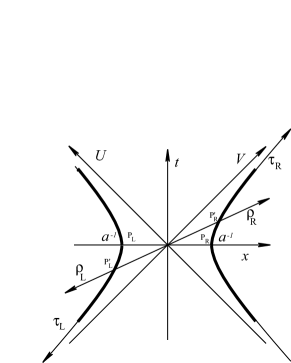
Figure 1: Minkowski and Rindler coordinates. The Minkowski time and space coordinates are $t$ and $x$; $V,U=t\pm x$ are the Minkowski light like coordinates; $\tau_{R}$, $\tau_{L}$ and $\rho_{R}$, $\rho_{L}$ denote the Rindler time and space coordinates in the right and left Rindler quadrants respectively. Note that $\tau_{R}$ increases toward the future, whereas $\tau_{L}$ increases toward the past. The uniformly accelerated oscillators follow the trajectories $\rho_{R}=a^{-1}$, and $\rho_{L}=a^{-1}$ which are indicated in the figure by bold curves. Due to Lorentz invariance, there is an infinite set of pairs of points for which the squared invariant distance between the oscillators is minimal, such as the pair $(P_{L},P_{R})$ or the pair $(P^{\prime}_{L},P^{\prime}_{R})$ indicated on the figure. The two oscillators only are entangled shortly after having reached positions where $\Delta s^{2}$ is minimal. For instance if the left oscillator is at $P_{L}$ (or $P^{\prime}_{L}$), the right oscillator should be along its worldline, slightly after $P_{R}$ (or $P^{\prime}_{L}$).

II The model

We parametrize 1+1 dimensional Minkowski space as

$$t=\rho_{R}\sinh a\,\tau_{R}\quad,\quad x=\rho_{R}\cosh a\,\tau_{R}\quad(|t|<x) \quad,$$ (1)

$$t=-\rho_{L}\sinh a\,\tau_{L}\quad,\quad x=-\rho_{L}\cosh a\,\tau_{L}\quad(x<-|t|) \quad.$$

Let us note that $\tau_{R}$ and $-\tau_{L}$ measure the proper time along the trajectories ($\rho_{R}=\rho_{L}=a^{-1}$) of the two oscilators. Later on we shall make use of the null coordinates

$$V = t+x=\left\{\begin{array}[]{ll}\ a^{-1}\exp av_{R}&\quad(|t|<\ x)\\ -a^{-1}\exp av_{L}&\quad(x<-|t|)\end{array}\right.\qquad,$$ (4)

$$U = t-x=\left\{\begin{array}[]{ll}-a^{-1}\exp au_{R}&\quad(|t|<x)\\ \ a^{-1}\exp au_{L}&\quad(x<-|t|)\end{array}\right.\qquad.$$ (7)

Note that with these definitions $\tau_{R}$, $v_{R}$ and $u_{L}$ increase toward the future, whereas $\tau_{L}$, $v_{L}$ and $u_{R}$ increase toward the past.

The problem of a single uniformly accelerated oscillator coupled to a massless field in $1+1$ dimensions has been extensively studiedRSG ; H ; MPB ; KK ; K . Here we generalise it to the case of two oscillators uniformly accelerated with the same acceleration $a$ in opposite Rindler quadrants. The action describing this system is

$$S = \int dxdt\frac{1}{2}[(\partial_{t}\phi)^{2}-(\partial_{x}\phi)^{2}]$$ (9)

$$+\int d\rho_{R}d\tau_{R}\delta(\rho_{R}-a^{-1})\left[\frac{m}{2}\left(\frac{dq_{R}}{d\tau_{R}}\right)^{2}-\frac{m}{2}\omega^{2}q_{R}^{2}+\epsilon\frac{dq_{R}}{d\tau_{R}}\phi(\tau_{R},a^{-1})\right]$$

$$-\int d\rho_{L}d\tau_{L}\delta(\rho_{L}-a^{-1})\left[\frac{m}{2}\left(\frac{dq_{L}}{d\tau_{L}}\right)^{2}-\frac{m}{2}\omega^{2}q_{L}^{2}-\epsilon\frac{dq_{L}}{d\tau_{L}}\phi(\tau_{L},a^{-1})\right]$$

where $q_{R}$ and $q_{L}$ are the internal coordinates of the oscillators; and $m,\omega$, $\epsilon$ are their mass, oscillation frequency, and coupling to the field. The momentum conjugate to the oscillator coordinates are

$$p_{R} = m\frac{dq_{R}}{d\tau_{R}}+\epsilon\phi(\tau_{R},a^{-1})\qquad,$$

$$p_{L} = -m\frac{dq_{L}}{d\tau_{L}}+\epsilon\phi(\tau_{L},a^{-1})\qquad.$$ (10)

The equations of motion are

$$\partial_{t}^{2}\phi-\partial_{x}^{2}\phi = \epsilon\frac{dq_{R}}{d\tau_{R}}\delta(\rho_{R}-a^{-1})+\epsilon\frac{dq_{L}}{d\tau_{L}}\delta(\rho_{L}-a^{-1})\qquad,$$

$$m\frac{d^{2}q_{R}}{d\tau_{R}^{2}}+m\omega^{2}q_{R}^{2} = -\epsilon\frac{d\phi(\tau_{R},a^{-1})}{d\tau_{R}}\qquad,$$

$$m\frac{d^{2}q_{L}}{d\tau_{L}^{2}}+m\omega^{2}q_{L}^{2} = +\epsilon\frac{d\phi(\tau_{L},a^{-1})}{d\tau_{L}}\qquad.$$ (11)

The first of these equations may be integrated to yield

$$\phi(x,t)=\phi^{0}(x,t)+\frac{\epsilon}{2}q_{R}(\tau_{Rret})+\frac{\epsilon}{2}q_{L}(\tau_{Lret})$$ (12)

where $\tau_{R,Lret}$ iare the values of $\tau_{R,L}$ at the intersection of the past light cone from $(x,t)$ with the right and left trajectories and where $\phi^{0}(x,t)$ is the free field operator, solution of $\partial_{t}^{2}\phi^{0}-\partial_{x}^{2}\phi^{0}=0$. We can reexpress the free field solution as

$$\phi^{0}(x,t)=\mathop{\phi^{0}}\limits_{{\leftarrow}}(t+x)+\mathop{\phi^{0}}\limits_{{\rightarrow}}(t-x)\qquad.$$ (13)

Inserting the solution for $\phi$ into the equation for $q_{R,L}$ yields the equations

$$m\frac{d^{2}q_{R}}{d\tau_{R}^{2}}+\frac{\epsilon^{2}}{2}\frac{dq_{R}}{d\tau_{R}}+m\omega^{2}q_{R} = -\epsilon\frac{d\phi^{0}(\tau_{R},a^{-1})}{d\tau_{R}}\qquad,$$

$$m\frac{d^{2}q_{L}}{d\tau_{L}^{2}}-\frac{\epsilon^{2}}{2}\frac{dq_{L}}{d\tau_{L}}+m\omega^{2}q_{L} = +\epsilon\frac{d\phi^{0}(\tau_{L},a^{-1})}{d\tau_{L}}\qquad.$$ (14)

The equation for $q_{R}$ can be integrated to yield

$$q_{R}(\tau_{R})=q_{0}(\tau_{R})-\int_{-\infty}^{\tau_{R}}d\tau_{R}^{\prime}\chi(\tau_{R}-\tau_{R}^{\prime})e\frac{d\phi^{0}(\tau_{R}^{\prime},a^{-1})}{d\tau_{R}^{\prime}}\qquad.$$ (15)

A similar solution obtains for $q_{L}$. Here $\chi$ is the retarded propagator of $q$, and $q_{0}$ is solution of $m\ddot{q_{0}}+\epsilon^{2}\dot{q_{0}}/2+m\omega^{2}q_{0}=0$. The free solution $q_{0}$ is exponentially damped. Henceforth we will neglect it. This corresponds to supposie that the oscillators were set into acceleration sufficiently far in the past and have reached thermal equilibrium with the Unruh heat bath.

Taking Fourier transforms, we can reexpress the solutions for the oscillators as

$$q_{R}(\tau_{R}) = i\frac{\epsilon}{m}\int d\lambda e^{-i\lambda\tau_{R}}\lambda\chi_{\lambda}\phi^{0}_{R}(\lambda)\qquad,$$

$$q_{L}(\tau_{L}) = i\frac{\epsilon}{m}\int d\lambda e^{+i\lambda\tau_{L}}\lambda\chi_{\lambda}\phi^{0}_{L}(\lambda)\qquad,$$

$$\chi_{\lambda} = \frac{-1}{\lambda^{2}-\omega^{2}+i\frac{\epsilon^{2}}{2m}\lambda}\qquad,$$

$$\phi^{0}_{R}(\lambda) = \int\frac{d\tau_{R}}{2\pi}e^{+i\lambda\tau_{R}}\phi^{0}(\tau_{R},a^{-1}),$$

$$\phi^{0}_{L}(\lambda) = \int\frac{d\tau_{L}}{2\pi}e^{-i\lambda\tau_{L}}\phi^{0}(\tau_{L},a^{-1})\qquad.$$ (16)

Since the equations of motion are linear, these expressions represent both the solutions to the classical and Heisenberg equations of motion. In what follows we will take the initial state of the field $\phi$ to be the vacuum state. The initial state of the oscillator is then irrelevant, since as we noted above, its state depends only on the state of the field.

A key point in our analysis is that the oscillators are then in a Gaussian state. Indeed the initial state of the field, the vacuum, is a Gaussian state. And the internal coordinates $q_{L,R}$ and conjugate momenta $p_{L,R}$ of the oscillators depend linearly on the field operator. Therefore the oscillators are also in a Gaussian state. This means that the reduced density matrix of the oscillators, obtained by tracing over the field degrees of freedom, is entirely characterised by the expectation values of the first and second moments of the oscillator variables. In particular, as we will review in the next section, these moments completely characterise the entanglement between the two oscillators.

It is immediate to obtain that the canonical variables have vanishing expectation value

$$\langle q_{R}\rangle=\langle q_{L}\rangle=\langle p_{R}\rangle=\langle p_{L}\rangle=0\ .$$

It is a more complicated task to compute the covariance matrix:

$$\sigma(\tau_{R},\tau_{L})=\left(\begin{array}[]{cccc}\langle q_{R}(\tau_{R})q_{R}(\tau_{R})\rangle&\langle\{q_{R}(\tau_{R}),p_{R}(\tau_{R})\}\rangle/2&\langle q_{R}(\tau_{R})q_{L}(\tau_{L})\rangle&\langle q_{R}(\tau_{R})p_{L}(\tau_{L})\rangle\\ \langle\{q_{R}(\tau_{R}),p_{R}(\tau_{R})\}\rangle/2&\langle p_{R}(\tau_{R})p_{R}(\tau_{R})\rangle&\langle p_{R}(\tau_{R})q_{L}(\tau_{L})\rangle&\langle p_{R}(\tau_{R})p_{L}(\tau_{L})\rangle\\ \langle q_{L}(\tau_{L})q_{R}(\tau_{R})\rangle&\langle q_{L}(\tau_{L})p_{R}(\tau_{R})\rangle&\langle q_{L}(\tau_{L})q_{L}(\tau_{L})\rangle&\langle\{q_{L}(\tau_{L}),p_{L}(\tau_{L})\}\rangle/2\\ \langle p_{L}(\tau_{L})q_{R}(\tau_{R})\rangle&\langle p_{L}(\tau_{L})p_{R}(\tau_{R})\rangle&\langle\{q_{L}(\tau_{L}),p_{L}(\tau_{L})\}\rangle/2&\langle p_{L}(\tau_{L})p_{L}(\tau_{L})\rangle\end{array}\right)$$ (17)

where $\{\cdot,\cdot\}$ is the anticommutator. The covariance matrix depends on the positions $\tau_{R}$ , $\tau_{L}$ of the two oscillators. The expectation values along a single trajectory, such as $\langle q_{R}(\tau_{R})q_{R}(\tau_{R})\rangle$, are independent of the position along the trajectory, since we have supposed that the oscillators have reached a stationary state. The expectation values between operators on opposite trajectories, such as $\langle q_{R}(\tau_{R})q_{L}(\tau_{L})\rangle$ depend only on $T=\tau_{R}-\tau_{L}$, since by boost invariance it depends only on the invariant distance between the two oscillators : $\Delta s^{2}=4\,a^{-2}\cosh a\,T/2$. Thus $\sigma$ is a function only of $T$. The detailed calculation of $\sigma$ will be carried out in section IV and in the appendix.

III Entanglement in continuous variable systems

Entanglement in continuous variable systems has been extensively studied, see for instance Simon ; GKLC ; Ad . We summarize here the results we will need in the remainder of the article.

Consider two oscillators whose phase space variables $(q_{R},p_{R})$ and $(q_{L},p_{L})$ obey the canonical commutation relations. It is convenient to group the phase space variables as $\vec{\xi}=(q_{R},p_{R},q_{L},p_{L})$. We can write the canonical commutation relations as

$$[\xi_{l},\xi_{m}]=i{\boldsymbol{\Omega}}_{lm}$$

where ${\boldsymbol{\Omega}}$ is the symplectic matrix

$${\boldsymbol{\Omega}}=\left(\begin{array}[]{cccc}0&1&0&0\\ -1&0&0&0\\ 0&0&0&1\\ 0&0&-1&0\end{array}\right)\qquad.$$ (18)

For any quantum state $\rho$ of the two oscillators, we can compute the first and second moments of its phase space variables

$$<\xi_{l}> = Tr\rho\xi_{l}$$ (19)

$${\boldsymbol{\sigma}}_{lm} = \frac{1}{2}Tr\rho\{\xi_{l}-<\xi_{l}>,\xi_{m}-<\xi_{m}>\}$$ (20)

where $\{,\}$ is the anticommutator. The covariance matrix of the oscillators is a real, symmetric, positive matrix, satisfying the constraint (which follows from positivity of the Hilbert Schmidt norm)

$${\boldsymbol{\sigma}}+i\frac{1}{2}{\boldsymbol{\Omega}}\geq 0\ .$$ (21)

In general the first and second moments are only a partial characterisation of the quantum state $\rho$. But in the particular case where $\rho$ is Gaussian, they completely characterise the state.

The correlation matrix ${\boldsymbol{\sigma}}$ allows one to study the entanglement of $\rho$. Denote by

$$\Lambda_{PT}=\left(\begin{array}[]{cccc}1&0&0&0\\ 0&1&0&0\\ 0&0&1&0\\ 0&0&0&-1\end{array}\right)$$

the matrix which realises the partial transpose. A necessary condition for entanglement of the two oscillators is

$$\Lambda_{PT}{\boldsymbol{\sigma}}\Lambda_{PT}+i\frac{1}{2}{\boldsymbol{\Omega}}\leq 0\ .$$ (22)

This condition is also sufficient if the oscillators are in a Gaussian state. It is convenient to rewrite this entanglement conditions as follows. Express the covariance matrix (17) as a bloc matrix

$$V=\left(\begin{array}[]{cc}{\bf A}&{\bf C}\\ {\bf C}^{T}&{\bf B}\end{array}\right)\qquad,$$ (23)

then eq. (22) is equivalent (when ${\bf A}={\bf B}$) to

$${\bf W}=\frac{1}{2}(\det[{\bf A}]-\det[{\bf C}])-\det[{\boldsymbol{\sigma}}]-\frac{1}{16}<0\qquad.$$ (24)

Below we will use the logarithmic negativity $E_{N}$ as quantitative measure of entanglement. It is defined as

$$E_{N}=\max[0,-\ln 2\eta^{-}]$$ (25)

where $\eta^{-}$ is the smallest symplectic eigenvalues of the matrix $\Lambda_{PT}{\boldsymbol{\sigma}}\Lambda_{PT}$ :

$$\eta^{\pm}=\frac{1}{\sqrt{2}}\left[\Sigma({\boldsymbol{\sigma}})\pm(\Sigma({\boldsymbol{\sigma}})^{2}-4det({\boldsymbol{\sigma}}))^{1/2}\right]$$ (26)

with $\Sigma({\boldsymbol{\sigma}})=det({\bf A})+det({\bf B})-2det({\bf C})$. The logarithmic negativity is an entanglement monotone. It is an upper bound on the distillable entanglement and a lower bound on the entanglement of formation. It measures the entanglement in units of entanglement bits (ebits), where one ebit is the entanglement present in a singlet state. Positivity of $E_{N}>0$ is a necessary condition for entanglement. In the particular case of Gaussian states it is both a necessary and sufficient condition.

IV Correlations between two uniformly accelerated oscillators

To compute the elements of the covariance matrix first we have to quantize the quantum field in Rindler coordinates and evaluate several Minkowskian vacuum expectation values. We refer to Unruh76 ; GO for detailed discussions of how to carry out these calculations, and summarize here very briefly the main points.

To lighten the formulas we shall chose our length unit so that :

$$a=1\qquad\qquad.$$ (27)

The quantum field being massless, it decomposes into left ($\leftarrow$) and right ($\rightarrow$) modes:

$$\boldsymbol{\Phi}(U,V)=\mathop{\Phi}\limits_{{\leftarrow}}(U)+\mathop{\Phi}\limits_{{\rightarrow}}(V)\qquad.$$ (28)

These modes themselves split into modes defined on the left (L) and right (R) Rindler quadrants. For example :

$$\mathop{\Phi}\limits_{{\leftarrow}}(U)={{\mathop{\Phi}\limits_{{\leftarrow}}}}_{R}(u_{R})+{{\mathop{\Phi}\limits_{{\leftarrow}}}}_{L}(u_{L})\qquad.$$ (29)

We can decompose these operators in terms of Rindler modes, and Rindler creation and destruction operators $b^{\dagger}_{u(v)_{R(L)}}(\lambda)$, $b_{u(v)_{R(L)}}(\lambda)$:

$${{\mathop{\Phi}\limits_{{\leftarrow}}}}_{R}(u) = \int_{0}^{\infty}\left(e^{-i\lambda u}b_{{u_{R}}}(\lambda)+e^{i\lambda u}b^{\dagger}_{{u_{R}}}(\lambda)\right)\frac{1}{\sqrt{4\,\pi\,\lambda}}d\lambda\qquad,$$ (30)

$${{\mathop{\Phi}\limits_{{\leftarrow}}}}_{L}(u) = \int_{0}^{\infty}\left(e^{i\lambda u}b_{{u_{L}}}(\lambda)+e^{-i\lambda u}b^{\dagger}_{{u_{L}}}(\lambda)\right)\frac{1}{\sqrt{4\,\pi\,\lambda}}d\lambda\qquad.$$ (31)

We emphasize the sign change in the arguments of the exponentials when we pass from the left to the right Rindler quadrant. It is the reflect of the opposite $u$-time orientation in these quadrants.
We can also decompose the field in terms of Minkowski modes and Minkowski creation and destruction operators $b^{\dagger}_{U(V)}(w)$, $b_{U(V)}(w)$:

$${\mathop{\Phi}\limits_{{\leftarrow}}}(U)=\int_{0}^{\infty}\left(e^{-i\,w\,U}b_{{U}}(w)+e^{+i\,w\,U}b^{\dagger}_{{U}}(w)\right)\frac{1}{\sqrt{4\,\pi\,w}}dw\qquad.$$ (32)

The link between these two decompositions is provided by standard Bogoljubov transformations. Using the Bogoljubov transformations one shows that the Minkowski vacuum is perceived by the uniformly accelerated observer as being populated by a thermal bath of Rindler quanta at temperature $T_{U}=\frac{a}{2\pi}$.

The Bogoljubov transformation also allows us to evaluate expectation values such as:

$$\frac{1}{2}\langle\{\tilde{\Phi}_{R}(\lambda),\tilde{\Phi}_{R}(\lambda^{\prime})\}\rangle = \langle\{{\mathop{\tilde{\Phi}}\limits_{\leftarrow}}_{R}(\lambda),\mathop{\tilde{\Phi}}\limits_{\leftarrow}{}_{R}(\lambda^{\prime})\}\rangle=\frac{1}{4\pi\lambda}\coth\lambda\pi\ \delta(\lambda+\lambda^{\prime})\qquad,$$ (33)

$$\frac{1}{2}\langle\{\tilde{\Phi}_{R}(\lambda),\tilde{\Phi}_{L}(\lambda^{\prime})\}\rangle = \langle\{{\mathop{\tilde{\Phi}}\limits_{\leftarrow}}_{R}(\lambda),\mathop{\tilde{\Phi}}\limits_{\leftarrow}{}_{L}(\lambda^{\prime})\}\rangle=\frac{1}{4\pi\lambda}\frac{1}{\sinh\lambda\pi}\delta(\lambda+\lambda^{\prime})\qquad.$$ (34)

These expressions are then used to evaluate the correlation matrix between position and momentum variables expressed as in eqs. (II ,10) :

$$qq_{RR}\equiv\langle q_{R}(\tau_{R})q_{R}(\tau_{R})\rangle = \frac{4\,\gamma\,\omega}{m}\int_{-\infty}^{+\infty}\frac{\lambda^{2}}{(\lambda-\bar{\Omega}_{+})(\lambda-\bar{\Omega}_{-})(\lambda-\Omega_{+})(\lambda-\Omega_{-})}\frac{\coth\lambda\pi}{4\,\lambda\,\pi}d\lambda$$ (35)

where we have introduced the notations:

$$\gamma=\frac{\epsilon^{2}}{4\,m\,\omega}\qquad,\qquad\Omega_{\pm}=\omega(\ i\gamma\pm\sqrt{1-\gamma^{2}})\qquad,\qquad\bar{\Omega}_{\pm}=\omega(-i\gamma\pm\sqrt{1-\gamma^{2}})\qquad.$$ (37)

As shown in the appendix, the integral over $\lambda$ can be carried out, giving a closed form for $qq_{RR}$.
Similarly the other correlators can be expressed as

$$qq_{RL}(T)\equiv\langle q_{R}(\tau_{R})q_{L}(\tau_{L})\rangle=-\frac{4\,\gamma\,\omega}{m}\int_{-\infty}^{+\infty}\frac{\lambda\,e^{-i\lambda T}}{(\lambda-\bar{\Omega}_{+})^{2}(\lambda-\bar{\Omega}_{-})^{2}}\frac{1}{4\,\pi\,\sinh\lambda\pi}d\lambda\qquad,$$ (38)

$$\frac{1}{2}\langle\{q_{R}(\tau_{R}),p_{R}(\tau_{R})\}\rangle=i\,4\,\gamma\,\omega^{2}\int_{-\infty}^{+\infty}\frac{1}{(\lambda-\bar{\Omega}_{+})(\lambda-\bar{\Omega}_{-})(\lambda-\Omega_{+})(\lambda-\Omega_{-})}\frac{\coth\lambda\pi}{4\,\pi}d\lambda=0\qquad,$$ (39)

$$qp_{RL}(T)\equiv\frac{1}{2}\langle\{q_{L}(\tau_{L})p_{R}(\tau_{R})\}\rangle=i\,4\,\gamma\,\omega^{3}\int_{-\infty}^{+\infty}\frac{e^{-i\lambda T}}{(\lambda-\bar{\Omega}_{+})^{2}(\lambda-\bar{\Omega}_{-})^{2}}\frac{1}{4\,\pi\,\sinh\lambda\pi}d\lambda\qquad.$$ (40)

In the last two expressions there is a pole at $\lambda=0$. We resolve the ambiguity in the resulting integrals by integrating in the sense of a principal part, thereby obtaining $0$ for the first integral and a closed form given in the appendix for $qp_{RL}$.

The computation of the momentum correlators are more delicate because they diverge due to the of a double pole at $\lambda=0$. We therefore introduce the infinite constant

$$K=\frac{\gamma\,m\,\omega}{\pi^{2}}\int\lambda^{-2}d\lambda\qquad,$$ (41)

and so obtain:

$$K+pp_{RR} \equiv \langle p_{R}(\tau_{R})p_{R}(\tau_{R})\rangle=4\,\gamma\,m\,\omega^{5}\int_{-\infty}^{+\infty}\frac{1}{(\lambda-\bar{\Omega}_{+})(\lambda-\bar{\Omega}_{-})(\lambda-\Omega_{+})(\lambda-\Omega_{-})}\frac{\coth\lambda\pi}{4\,\lambda\,\pi}d\lambda\qquad,$$ (42)

$$K+pp_{RL}(T) \equiv \frac{1}{2}\langle\{p_{R}(\tau_{R}),p_{L}(\tau_{L})\}\rangle=4\,\gamma\,m\,\omega^{5}\int_{-\infty}^{+\infty}\frac{e^{-i\lambda T}}{(\lambda-\bar{\Omega}_{+})^{2}(\lambda-\bar{\Omega}_{-})^{2}}\frac{1}{4\,\lambda\,\pi\,\sinh\lambda\pi}d\lambda\qquad,$$ (43)

where $pp_{RR}$ and $pp_{RL}(T)$ are finite quantities whose closed forms are given in the appendix.

We may therefore write the correlation matrix as

$${\boldsymbol{\sigma}}=\left(\begin{array}[]{cccc}qq_{RR}&0&qq_{RL}(T)&qp_{RL}(T)\\ 0&K+pp_{RR}&qp_{RL}(T)&K+pp_{RL}(T)\\ qq_{RL}(T)&qp_{RL}(T)&qq_{RR}&0\\ qp_{RL}(T)&K+pp_{RL}(T)&0&K+pp_{RR}\end{array}\right)\qquad.$$ (44)

In this expression, except for $K$ which is infinite, all the other terms are finite functions, depending only of the dimensionless parameters $\omega$, $\gamma$, $T$, which can be interpreted as follows. The parameter $\omega$ is the ratio between the transition frequency of the oscillator and the acceleration $a$: $\omega\equiv\frac{\omega}{a}=\frac{\omega}{2\pi T_{U}}$ where $T_{U}$ is the Unruh temperature. When $\omega>2\pi$ the probability that the oscillator is excited will be exponentially small. We therefore expect any entanglement between the oscillators to disapear for large values of $\omega$ (since entanglement requires superpositions between several states). The parameter $\gamma\equiv\frac{\epsilon^{2}}{4\,m\,\omega}$ is the ratio between the line width $\Gamma=\frac{\epsilon^{2}}{4\,m}$ (the inverse lifetime) of the first excited state of the oscillator and its transition frequency $\omega$. When $\gamma>1$ the oscillator is strongly coupled to the field, whereas when $\gamma<1$ the oscillator is weakly coupled to the field. This translates in the Heisenberg equations of motion into the difference between the free solution being over damped or oscillating as it decays. In what follows we shall only consider the regime $\gamma<1$. Finally $T\equiv a(\tau_{R}-\tau_{L})$ is the difference of the Rindler times along the two trajectories, in units of the inverse acceleration. It measures the Lorentz invariant distance of points on the two trajectories: $\Delta s^{2}=4\,a^{-2}\cosh a\,T/2$.

We have checked numerically that the correlation matrix obeys the positivity constraint eq. (21). Indeed when inserting eq. (44) into eq. (21) we find that the resulting matrix has one infinite positive eigenvalue, and three finite eigenvalues which we found to be positive using the procedure outlined in the appendix.

Similarly we can consider the condition of positive partial transpose eq. (22). Once more, inserting eq. (44) into eq. (22) we find that the resulting matrix has one infinite positive eigenvalue, and three finite eigenvalues. When one of these eigenvalues becomes negative the state is entangled. We have also computed the logarithmic negativity $E_{N}$ which quantifies the degree of entanglement present in the system. We find that logarithmic negativity is always finite and independent of $K$ (see eq.(56)).

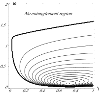
Figure 2: Maximum entanglement between the oscillators, as a function of the dimensionless parameters $\gamma$ and $\omega$. The outer line is the frontier of the region where the oscillators get entangled. The contour lines correspond to increases in the logarithmic negativity $E_{N}$ in steps of $0.1$. The maximum entanglement occurs for $\gamma\simeq 0.703$, $\omega\simeq 0.0845$ when $E_{N}=1.406$.

Thus, even though the fluctuations of the oscillators coupled to the field are infinite, since the momentum correlators are infinite, the model is well defined. In particular the quantity we are interested in, the entanglement between the two oscillators, is always finite.

We have computed the entanglement between the two oscillators as a function of $T$ for different values of $\omega$ and $\gamma<1$. We find that there are only specific pairs of values $(\gamma,\omega)$ for which the detectors become entangled. In Fig. 2 we have plotted the pairs of values of $(\gamma,\omega)$ for which the detector gets entangled. Note that our numerical analysis indicates that the region where entanglement occurs does not touch the axes $\gamma=0$ and $\omega=0$. This is interesting since these axes correspond to the domain of validity of perturbation theory. Indeed the perturbative limit should arise when $\epsilon\to 0$, $m$ fixed which corresponds to $\gamma\omega=\epsilon^{2}/m\to 0$. Thus the entanglement between two uniformly accelerated oscillators in opposite Rindler quadrants is a non perturbative phenomena.

In Fig. 2 we have also plotted the degree of entanglement between the two oscillators as a function of $(\gamma,\omega)$. We see that the entanglement is maximum for $\gamma\simeq 0.703$, $\omega\simeq 0.0845$ whereupon the logarithmic negativity reaches the value $E_{N}=1.406$, see Fig. 3 for further discussion of this case.

We have also computed how the entanglement between the two oscillators evolves as a function of $T$. For all values of the parameters, we find that the entanglement only appears when $T>0$. That is the entanglement only gets established after a configuration of closest approach ($T=\tau_{R}-\tau_{L}=0$) has been realized. The entanglement then increases, reaches a maximum, decreases and goes zero at a finite value of $T$. We can understand this as follows. The oscillators emit and absorb quanta that are packets localised in frequency and time (for instance if $\gamma<<1$ then $\Delta\lambda\simeq\epsilon^{2}/2m$ and $\Delta\tau\simeq(\epsilon^{2}/2m)^{-1}$). These quanta are only correlated around configurations of closest approach $T\simeq 0$. It takes some time to establish correlations between the two detectors, which is why the entanglement only appears for $T>0$. At late times the quanta exchanged between the two oscillators are no longer correlated. The entanglement is gradually erased and finally disappears. As illustration in Fig. 3 we have plotted how the entanglement between the two detectors evolves as a function of $T$ for the value of $\gamma$ and $\omega$ for which entanglement is maximal

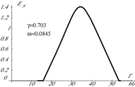
Figure 3: Evolution of the logarithmic negativity $E_{N}$ between the two oscillators as a function of $T=\tau_{R}-\tau_{L}$ for the values $\gamma=0.703$, $\omega=0.0845$ for which it reaches its maximal value of $1.406$. In these units the period of the oscillator is $2\pi/\omega\simeq 74$, and the ”lifetime” of the first excited state of the oscillator is $\Gamma^{-1}=(\gamma\omega)^{-1}=17$. (We put quotes because the concept of lifetime is not well defined when it is smaller than the oscillation period, although it serves as a useful guiding concept for understanding what are the different time scales involved). The oscillator is thus entangled for less than one oscillation period, and during this time it exchanges several quanta with the Unruh heat bath. Note also that in this case the Boltzman factor $e^{-2\pi\omega}\simeq 0.6$ is of order 1 which implies that several of the oscillator levels have significant probability of being populated -this is necessary since $E_{N}>1$ requires a system with dimension greater than 2-. The shapes of the curves for other values of $\gamma$ and $\omega$ are similar, except that the maximum entanglements reached are smaller, and that the times at which these maxima are reached are different.

Note that because of boost invariance there is in fact an infinite set of pairs of locations for which the oscillators are entangled. Indeed if we look at one oscillator at a specific value of its proper time $\tau_{L(R)}=\tau^{\star}$, it is only entangled with the other for a finite interval of proper time starting slightly after $\tau_{R(L)}=\tau^{\star}$. This is depicted schematically in Fig. 1.

In summary we have studied the entanglement between two uniformly accelerated oscillators in 1+1 dimensional Minkowsky space time coupled to a massless scalar field. This model is exactly soluble. It allows us to study the case where both detectors are in thermal equilibrium with the field. It also allows us to study the case where the detectors are strongly coupled to the field. We find that there are some choices of parameters and of positions along the trajectories for which the two detectors get entangled. The maximum entanglement we find is slightly larger than $1.4$ entanglement bits.

V Appendix: Details of Calculations

We group here some of the calculations that are behind our main results.

V.1 Explicit expressions for the correlation matrix elements

Here we give explicit expressions for the correlators, which are expressed in terms of integrals in the main text. Specifically, upon carrying out the integrals in eqs. (35,38,40,42,43), one finds

$$\langle q_{R}(\tau_{R})q_{R}(\tau_{R})\rangle = \frac{\sinh\left(2\pi\sqrt{1-\gamma^{2}}\omega\right)}{2\sqrt{1-\gamma^{2}}\omega\left(\cosh\left(2\pi\sqrt{1-\gamma^{2}}\omega\right)-\cos(2\pi\gamma\omega)\right)}-\frac{2\gamma\omega}{\pi}\sum_{n=1}^{\infty}\frac{n}{\left(n^{2}+\omega^{2}\right)^{2}-4n^{2}\gamma^{2}\omega^{2}}\qquad,$$ (45)

$$\langle q_{R}(\tau_{R})q_{L}(\tau_{L})\rangle=\frac{\gamma\,\theta(T)\,e^{-T\gamma\omega}}{\left(1-\gamma^{2}\right)^{3/2}\omega}\Re\left[\frac{e^{iT\sqrt{1-\gamma^{2}}\omega}\left((1-\gamma^{2}+i\gamma\sqrt{1-\gamma^{2}})\omega(T+i\pi\,\coth\left[\pi\omega(\sqrt{1-\gamma^{2}}+i\gamma)\right])-\gamma\right)}{\sinh\left[\pi(\sqrt{1-\gamma^{2}}+i\gamma)\omega\right]}\right]$$

$$+\frac{2\gamma\omega}{\pi}\left(\theta[T]\sum_{n=1}^{\infty}\frac{(-1)^{n}ne^{-nT}}{\left(n^{2}-2\gamma\omega n+\omega^{2}\right)^{2}}+\theta[-T]\sum_{n=1}^{\infty}\frac{(-1)^{n}ne^{nT}}{\left(n^{2}+2\gamma\omega n+\omega^{2}\right)^{2}}\right)\qquad,$$ (46)

$$\frac{1}{2}\langle\{ q_{L}(\tau_{L})p_{R}(\tau_{R})\}\rangle=-\frac{\gamma\,\theta(T)\,e^{-T\gamma\omega}}{2\left(1-\gamma^{2}\right)^{3/2}}\Re\left[\frac{e^{iT\sqrt{1-\gamma^{2}}\omega}\left(1+\sqrt{1-\gamma^{2}}\omega(\pi\,\coth\left[\pi\omega(\sqrt{1-\gamma^{2}}+i\gamma)\right]-iT)\right)}{\sinh\left[\pi(\sqrt{1-\gamma^{2}}+i\gamma)\omega\right]}\right]$$

$$\quad\quad\quad+\frac{2\gamma\omega^{3}}{\pi}\left[\theta[T]\left(\sum_{n=1}^{\infty}\frac{(-1)^{n}e^{-nT}}{\left(n^{2}-2\gamma\omega n+\omega^{2}\right)^{2}}+\frac{1}{2\omega^{4}}\right)-\theta[-T]\left(\sum_{n=1}^{\infty}\frac{(-1)^{n}e^{nT}}{\left(n^{2}+2\gamma\omega n+\omega^{2}\right)^{2}}+\frac{1}{2\omega^{4}}\right)\right]\quad,$$

$$\langle p_{R}(\tau_{R})p_{R}(\tau_{R})\rangle = K+\frac{\omega\left(\left(1-2\gamma^{2}\right)\sinh\left(2\pi\sqrt{1-\gamma^{2}}\omega\right)-2\gamma\sqrt{1-\gamma^{2}}\sin(2\pi\gamma\omega)\right)}{2\sqrt{1-\gamma^{2}}\left(\cosh\left(2\pi\sqrt{1-\gamma^{2}}\omega\right)-\cos(2\pi\gamma\omega)\right)}$$ (48)

$$+\frac{2\gamma\omega^{5}}{\pi}\sum_{n=1}^{\infty}\frac{1}{n\left(\left(n^{2}+\omega^{2}\right)^{2}-4n^{2}\gamma^{2}\omega^{2}\right)}\qquad,$$

$$\frac{1}{2}\langle\{p_{R}(\tau_{R}),p_{L}(\tau_{L})\}\rangle=K+\frac{\gamma\,\theta(T)\,e^{-T\gamma\omega}}{\left(1-\gamma^{2}\right)^{3/2}}\ \Re\left[e^{iT\sqrt{1-\gamma^{2}}\omega}\left(\frac{3\,\gamma-2i\,\gamma^{3}+2\,(1-\gamma^{2})^{3/2}}{\sinh\left[\pi(\sqrt{1-\gamma^{2}}+i\gamma)\omega\right]}\right.\right.$$ (49)

$$\qquad\qquad\qquad\qquad\qquad\qquad\left.\left.+\frac{(1-\gamma^{2}-\,i\,\gamma\sqrt{1-\gamma^{2}})\omega\left(T+i\pi\,\coth\left[\pi\omega(\sqrt{1-\gamma^{2}}+i\gamma)\right]\right)}{\sinh\left[\pi(\sqrt{1-\gamma^{2}}+i\gamma)\omega\right]}\right)\right]$$

$$+\frac{\gamma\omega^{5}}{\pi}\left[\theta[T]\left(2\sum_{n=1}^{\infty}\frac{(-1)^{n}e^{-nT}}{n\left(n^{2}-2\gamma\omega n+\omega^{2}\right)^{2}}+\frac{4\gamma-T\omega}{\omega^{5}}\right)+\theta[-T]\left(2\sum_{n=1}^{\infty}\frac{(-1)^{n}e^{nT}}{n\left(n^{2}+2\gamma\omega n+\omega^{2}\right)^{2}}-\frac{4\gamma-T\omega}{\omega^{5}}\right)\right]\qquad.$$

V.2 Positivity and Entanglement

Positivity of the Hilbert space inner product implies the positivity of the matrix ${\boldsymbol{\sigma}}+i{\boldsymbol{\Omega}}$, see eq. (21). We checked that this is indeed the case as one of the eigenvalue of this matrix is infinite $=K$, while the three other are given by the eigenvalues of the matrix acting on the orthogonal space to the eigenvector of this infinite eigenvalue:

$$\left(\begin{array}[]{ccc}{qq_{RR}}-{qq_{RL}}&\frac{i}{2}-{qp_{RL}}&0\\ -\frac{i}{2}-{qp_{RL}}&{pp_{RR}}-\ {pp_{RL}}&0\\ 0&0&{qq_{RL}}+{qq_{RR}}\end{array}\right)$$ (50)

The three eigenvalues of this matrix are easy to compute. Using the above expressions for the correlators, we have checked numerically that they are positive, as expected.

The criterium to put into evidence entanglement for a Gaussian system consists to show the occurence of negative eigenvalue in the partially transposed of the previous correlation matrix, i.e. the negativity of the matrix

$${\boldsymbol{\sigma}^{PT}+i\Omega}=\left(\begin{array}[]{cccc}qqRR&qpRR+\frac{i}{2}&qqRL&-qpRL\\ qpRR-\frac{i}{2}&K+ppRR&qpRL&-K-ppRL\\ qqRL&qpRL&qqRR&-qpRR+\frac{i}{2}\\ -qpRL&-K-ppRL&-qpRR-\frac{i}{2}&K+ppRR\end{array}\right)\qquad.$$ (51)

Here again we find that one of the eigenvalues of this matrix is infinite $=K$. The computation of the three other eigenvalues is less obvious than in the previous case. First we may perform a symplectic transformation, using the matrix

$$\left(\begin{array}[]{cccc}\frac{1}{\sqrt{2}}&0&-\frac{1}{\sqrt{2}}&0\\ 0&\frac{1}{\sqrt{2}}&0&-\frac{1}{\sqrt{2}}\\ \frac{1}{\sqrt{2}}&0&\frac{1}{\sqrt{2}}&0\\ 0&\frac{1}{\sqrt{2}}&0&\frac{1}{\sqrt{2}}\end{array}\right)$$ (52)

to obtain the expression

$$\left(\begin{array}[]{cccc}{qqRR}-{qqRL}&\frac{i}{2}&0&-{qpRL}\\ -\frac{i}{2}&2K+{ppRL}+{ppRR}&{qpRL}&0\\ 0&{qpRL}&{qqRL}+{qqRR}&\frac{i}{2}\\ -{qpRL}&0&-\frac{i}{2}&{ppRR}-{ppRL}\end{array}\right)$$ (53)

from which it is easy to isolate the eigenspace attached to the infinite eigenvalue and its orthogonal subspace. But to obtain the remaining three eigenvalues, i.e. the eigenvalues of the reduced matrix

$${\bf V}=\left(\begin{array}[]{ccc}{qqRR}-{qqRL}&0&-{qpRL}\\ 0&{qqRL}+{qqRR}&\frac{i}{2}\\ -qpRL&-\frac{i}{2}&{ppRR}-{ppRL}\end{array}\right)\ ,$$ (54)

we have to use (in principle) the general Cardan formula. We have performed such an analysis numerically. We have also used the criteria eq. (22) which in the present case reduces to

$$\lim_{K\to\infty}K^{-1}{\bf W}=-2\det[{\bf V}]\qquad.$$ (55)

Finally the smallest symplectic eigenvalue of the partial transpose of $\boldsymbol{\sigma}$ can be expressed as:

$$\eta_{-}=\sqrt{\frac{1}{4}+\frac{\det[{\bf V}]}{(qqRR-qqRL)}}\ .$$ (56)

It is independent of $K$. The expressions (55) and (56) were used to compute numerically the results discussed in the main text.

References

- (1) W. G. Unruh, Phys. Rev. D 14 (1976) 870.
- (2) N. D. Birrell, P. C. W. Davies, Quantum Fields in Curved Space, Cambridge University Press, Cambridge, 1982
- (3) R. Brout, S. Massar, R. Parentani, Ph. Spindel, Physics Reports 260 (1995) 329
- (4) S. J. Summers, R. F. Werner Phys. Lett. A 110 (1985) 257-259
- (5) S. J. Summers, R. F. Werner J. Math. Phys. 28 (1987) 2440-2447
- (6) S. J. Summers, R. F. Werner J. Math. Phys. 28 (1987) 2448-2456
- (7) S. J. Summers, R. F. Werner Commun. Math. Phys. 110 (1987) 247-259
- (8) S. J. Summers, R. F. Werner Ann. Inst. H. Poincar A 49 (1988) 215-243
- (9) H. Halvorson and R. Clifton, Bell correlation between arbitrary local algebras in quantum field J. Math. Phys. 41 (2000) 1711 [arXiv:math-ph/9909013].
- (10) B. Reznik, vacuum,” Found. Phys. 33 (2003) 167 [arXiv:quant-ph/0212044].
- (11) B. Reznik, A. Retzker, J. Silman, Phys. Rev. A71 (2005) 042104
- (12) J. Silman, B. Reznik, Phys. Rev. A 71, 054301 (2005)
- (13) D. J. Raine, D. W. Sciama, P. G. Grove, Proc. R. Soc. London A435, 205 (1991)
- (14) F. Hinterleitner, Ann. Phys. (N.Y.) 226 (1993) 165
- (15) S. Massar, R. Parentani and R. Brout, 1992,” Class. Quant. Grav. 10 (1993) 385.
- (16) H.-C. Kim and J. K. Kim, Phys. Rev. D 56 (1997) 3537
- (17) H.-C. Kim, Phys. Rev. D 59 (1999) 064024
- (18) W. G. Unruh, W. H. Zurek, Phys. Rev. D 40 (1989) 1071
- (19) W. G. Unruh, R. M. Wald, Phys. Rev. D 52 (1995) 2176
- (20) J. R. Anglin, R. Laflamme, W. H. Zurek, J. P. Paz, Phys. Rev. D 52 (1995) 2221
- (21) A. Einstein, B. Podolsky, and R. Rosen, Phys. Rev. 47, 777 (1935)
- (22) R. Simon, Phys. Rev. Lett. 84 (2000) 2726; see also R. Simon Separability criterion for gaussian states, in Quantum In formation with Continuous Variables, eds S. L. Braunstein and A. K. Pati, Kluver Academic publishers, Netherlands, (2003) 155-172
- (23) G. Giedke, B. Kraus, M. Lewenstein, J. I. Cirac, Phys. Rev. Lett. 87 (2001) 167904
- (24) G. Adesso, A. Serafini, F. Illuminati, Phys. Rev. A 70 (2004) 022318