Hofstadter Butterfly Diagram in Noncommutative Space

Abstract

We study an energy spectrum of electron moving under the constant magnetic field in two dimensional noncommutative space. It take place with the gauge invariant way. The Hofstadter butterfly diagram of the noncommutative space is calculated in terms of the lattice model which is derived by the Bopp’s shift for space and by the Peierls substitution for external magnetic field.

We also find the fractal structure in new diagram. Although the global features of the new diagram are similar to the diagram of the commutative space, the detail structure is different from it.

The recent development of the noncommutaitve space (NC) physics has shown the interesting results in the theoretical point of view. Most development has been made in the string theory conn_doug_schw ; sei_wit ; douglas_rev . The string theory is believed to be a ruling theory of the quantum gravity. In the quantum gravity, space and time coordinates should be fluctuating. As the result there exist some scale $\theta$ in the theory. Therefore, space and time coordinate should be discretize in units of $\theta$. This means that the space of the quantum gravity should be described in terms of new geometry instead of the Riemann geometry.

The noncommutative geometry is the leading candidate for the geometry of quantum gravity and is naturally formulated in terms of D-branes. The coordinates of this geometry satisfy the commutation relation,

$$[\hat{x}_{\mu},\,\hat{x}_{\nu}]_{\star}=i\theta_{\mu\nu},\quad\theta_{\mu\nu}=-\theta_{\nu\mu}$$ (1)

where $\theta_{\mu\nu}$ is a noncommutative parameter which is related to the string tension $\alpha^{\prime}$. In noncommutative space, the product between functions becomes $\star$-product;

$$f(x)\star g(x) =\exp\left[\dfrac{i}{2}\theta_{\mu\nu}\dfrac{\partial}{\partial\xi^{\mu}}\dfrac{\partial}{\partial\zeta^{\nu}}\right]f\left(x+\xi\right)g\left(x+\zeta\right)\biggl{|}_{\xi=\zeta=0}$$

$$=f(x)g(x)+\dfrac{i}{2}\theta_{\mu\nu}\partial_{\mu}f\partial_{\nu}g+\textrm{O}(\theta^{2})$$ (2)

For example, two dimensional noncommutative coordinate $\hat{\bm{r}}=(\hat{x},\hat{y})$ satisfies

$$\left[\hat{x},\,\hat{y}\right]_{\star}=\hat{x}\star\hat{y}-\hat{y}\star\hat{x}=i\theta,$$

where we take $\theta_{\mu\nu}=\theta\epsilon_{\mu\nu}$ and $\epsilon_{\mu\nu}$ is two rank antisymmetric tensor with $\epsilon_{12}=1$. Further,

$$\left[\hat{x},\,\hat{x}\right]_{\star}=0,\quad\left[\hat{y},\,\hat{y}\right]_{\star}=0.$$

This means that a particle has nontrivial phase shift only when the electron comes back to starting point with different path in the noncommutative space.

The noncommutative space ($\hat{\bm{r}}$) is reformulated in terms of commutative coordinate ($\bm{r}$) with the Bopp’s shifts curt_fair_zach .

$$\hat{x}=x-\dfrac{\theta}{2}p_{y},\quad\hat{y}=y+\dfrac{\theta}{2}p_{x},$$ (3)

where $x,y,p_{x},p_{y}$ satisfy the following commutation relations,

$$[x,\,p_{x}]=i,\quad[y,\,p_{y}]=i,\quad[x,\,y]=0,\quad[p_{x},\,p_{y}]=0.$$

In the literature, the noncommutative parameter can be interpreted to an external magnetic field. This is an intersting analogy between the noncommutative parameter and the external magnetic field. But our approach is distinct from it. In this Letter, we consider electron in the noncommutative space with external noncommutative magnetic field.

In the noncommutative space, U(1) gauge theory (QED) becomes a noncommutative U(1) gauge theory (NCQED). The NCQED model has a local NC U(1) gauge symmetry. The NC gauge transformation of NC fermion $\hat{\psi}$ and the NC gauge field $\hat{A}_{\mu}$ is given by

$$\hat{\psi}^{\prime}=e^{-i\lambda}_{\star}\star\hat{\psi},$$ (4)

where

$$U=e^{-i\lambda}_{\star}\equiv 1-i\lambda+\dfrac{(-i)^{2}}{2!}\lambda\star\lambda+\cdots$$ (5)

and

$$\hat{A}_{\mu}^{\prime}=U\star A_{\mu}\star U^{\dagger}+\dfrac{i}{e}U\star\partial_{\mu}U^{\dagger}.$$ (6)

It is important to note that the NC magnetic field is not a gauge invariant object like as QCD because the (NC) field strength $\hat{F}_{\mu\nu}$ is not gauge invariant. Therefore, we must take care of the gauge invariance of the physical observable more carefully in NCQED than in QED.

It is interesting to enlarge the application of the noncommutative theory to quantum mechanics curt_fair_zach ; duval_horv ; nair_pol ; fal_gam_loe_roj_prd66 ; chain_pres_shek_ture ; dayi_jellal , e.g. Landau level problem duval_horv ; nair_pol ; dayi_jellal ; fal_gam_loe_roj_prd66 . The continuous spectrum of an free electron becomes discrete spectrum when the constant magnetic field is switched on. Further, to take a lattice formulation, we find the fractal structure in the Hofstadter butterfly diagram hofstadter ; hiramoto_kohmoto_rev .

In the noncommutative space, the Hamiltonian of the electron should be given by

$$H_{nc}=\dfrac{1}{2m}\left(\hat{\bm{p}}+e\hat{\bm{A}}(\hat{\bm{r}})\right)^{2}.$$ (7)

In terms of the Bopp’s shift formulation, the NC U(1) gauge field $\hat{\bm{A}}$ is mapped to the gauge field $\bm{A}$ in the commutative space fal_gam_loe_roj_prd66 as

$$\hat{A}_{j}\rightarrow A_{j}-\dfrac{1}{2}\theta_{ab}\partial_{a}A_{j}p_{b}.$$ (8)

Therefore, the Hamiltonian can be rewritten in terms of the commutative coordinates as

$$H_{nc}=\dfrac{1}{2m}\left(p_{j}+eA_{j}-\dfrac{e}{2}\theta_{ab}\partial_{a}A_{j}p_{b}\right)^{2}$$ (9)

To take the symmetric gauge,

$$\bm{A}=\left(-\dfrac{B}{2}y,\,\dfrac{B}{2}x,0\right),$$ (10)

the Hamiltonian becomes dayi_jellal

$$H=\dfrac{1}{2m}\left(\Pi_{x}^{2}+\Pi_{y}^{2}\right),$$

where

$$\Pi_{x}=\xi_{\theta}^{-2}p_{x}-\dfrac{eB}{2}y,\quad\Pi_{y}=\xi_{\theta}^{-2}p_{y}+\dfrac{eB}{2}x$$

and

$$\xi_{\theta}^{-2}\equiv 1-\dfrac{eB\theta}{4}.$$ (11)

In this case, the commutation relations become

$$\left[x,\,\Pi_{x}\right]=i\xi_{\theta},\quad\left[y,\,\Pi_{y}\right]=i\xi_{\theta},$$ (12a)

$$\left[\Pi_{x},\,\Pi_{y}\right]=-ieB\xi_{\theta}^{-2}.$$ (12b)

Further, the Hamiltonian can be expressed in terms of a harmonic oscillator dayi_jellal ,

$$H=\dfrac{eB}{m}\xi_{\theta}^{-2}\left(a^{\dagger}a+\dfrac{1}{2}\right),\quad\left[a,\,a^{\dagger}\right]=1$$ (13)

with the transformation,

$$\Pi_{x}=\dfrac{\xi_{\theta}^{-1}}{i}\sqrt{\dfrac{eB}{2}}\left(a-a^{\dagger}\right),\quad\Pi_{y}=\xi_{\theta}^{-1}\sqrt{\dfrac{eB}{2}}\left(a+a^{\dagger}\right).$$

This means that the energy spectrum of the electron in the noncommutative space is discretized and the Landau level like spectrum is also emerged in noncommutative space. The gap of the energy spectrum is given by

$$E=\dfrac{eB}{m}\xi_{\theta}^{-2}.$$ (14)

Note that the Landau level in the noncommutative space is different from the commutative case by a factor $\xi_{\theta}^{-2}$. That is, it is expected that the difference of the Hofstadter diagram between the commutative and the noncommutative case emerge.

In the above, however, we chose the symmetric gauge to derive the Hamiltonian. In the gauge theory, a physical observable must be gauge invariance quantity. In the commutative space, we can easily verify that the spectrum of the Landau level and the relation

$$[\Pi_{x},\Pi_{y}]\psi=-ieB\psi$$ (15)

are gauge invariance. On the other hand, it is not obvious that the commutation relation eq.(12b) and the energy eq.(14) are gauge invariant.

It can be shown in the order of $\theta(\theta\ll 1)$ that after the gauge transformation

$$D_{\mu}^{\prime}\star\psi^{\prime}=e^{-i\lambda}\star\bigl{(}D_{\mu}\star\psi\bigr{)},$$ (16)

where $D_{\mu}=\partial_{\mu}+ieA_{\mu}$ is the covariant derivative. Therefore, we can find that

$$D_{\mu}^{\prime}\star\bigl{(}D_{\nu}^{\prime}\star\psi^{\prime}\bigr{)}=e^{-i\lambda}\star\biggl{(}D_{\mu}\star\bigl{(}D_{\nu}\star\psi\bigr{)}\biggr{)}.$$ (17)

It is important to note here that the order of the star product with a differential operator $\partial_{\mu}$ is important. From eq.(17), we can easily prove that

$$[D_{\mu},D_{\nu}]_{\star}\diamond\psi=c_{0}\psi$$ (18)

is NC U(1) gauge invariant when $c_{0}$ is constant. Here, for convenience, we introduced $\diamond$ operation between $\Phi_{1}(\equiv\phi_{1}\star\phi_{2})$ and $\Psi$ as

$$\Phi\diamond\Psi\equiv\biggl{(}\phi_{1}\star\bigl{(}\phi_{2}\star\Psi\bigr{)}\biggr{)}.$$ (19)

To take the symmetric gauge eq(10), we have the relation

$$[\Pi_{x},\Pi_{y}]_{\star}\diamond\psi=-ieB\left(1-\dfrac{eB\theta}{4}\right)\psi$$ (20)

where $\bm{\Pi}\equiv-i\bm{D}$. Further, the NC Schrödinger equation of the electron whose energy is $E_{0}$,

$$H\diamond\psi=E_{0}\psi,\qquad H=-\dfrac{1}{2m}\bm{D}\star\bm{D}$$ (21)

is gauge invariant. Accordingly, the commutation relation eq.(20) and the energy of electron is invariant under the NC U(1) gauge transformation. More detail discussion of the gauge invariance will be found in taka_yama

Finally, we should conclude that the electron moving under the constant magnetic field $B$ in the noncommutative space is equivalent to the electron moving under the constant magnetic field $B\xi_{\theta}^{-2}$ in the commutative space,

$$eB\longrightarrow eB\left(1-\dfrac{eB\theta}{4}\right).$$ (22)

Now, we consider the Hofstadter butterfly diagram in the noncommutative space. The Hofstadter butterfly diagram is the relation between the energy spectrum of lattice Hamiltonian of electron and the flux $\phi=eB$. It gives the Landau level in the continuous limit thouless_83prb .

Electrons in a two-dimensional lattice subject to a uniform magnetic field show extremely rich and interesting behavior. Usually a solid with well localized atomic orbits is modeled by the tight-binding Hamiltonian and the effect of the magnetic field is included by the Peierls substitution. To characterize the system, one can use the flux per plaquette, $\phi$. When $\phi$ is rational, the single-particle Schrödinger equation is reduced to the Harper’s equation harper ; wannier . The equation appears in many different physical contexts ranging from the quasiperiodic systems hiramoto_kohmoto_rev to quantum Hall effects tknn ; ntw . When $\phi$ is irrational, the spectrum is known to have an rich structure like the Cantor set and to exhibit a multifractal behavior hofstadter ; hiramoto_kohmoto_rev .

The lattice version of the Hamiltonian of the electron can be formulated from the continuum Hamiltonian in terms of the Bopp’s shift for space and the Peierls substitution for the external magnetic field. In this respect, the lattice Hamiltonian can be described by

$$H=T_{x}+T_{y}+T_{x}^{\dagger}+T_{y}^{\dagger},$$ (23)

where $T_{\mu}$ is translation operator which is defined as

$$T_{\mu}=e^{i\sqrt{\frac{a}{4m}}\Pi_{\mu}},$$

where $a$ is lattice spacing. We can verify that

$$T_{x}(a)T_{y}(b)=e^{iab/(\ell^{2}\xi_{\theta}^{2})}T_{y}(b)T_{x}(a),$$ (24)

where $\ell^{-2}=eB$. Therefore, the path ordering integral of the plaquette

$$\textrm{P}\exp\left(i\oint_{C}\!dx_{\mu}\,\Pi_{\mu}\right)=T_{x}(a)T_{y}(b)T_{x}^{-1}(a)T_{y}^{-1}(b)$$

becomes

$$\textrm{P}\exp\left(i\oint_{C}\!dx_{\mu}\,\Pi_{\mu}\right)=\exp\left(i\dfrac{2\pi\Phi}{\varphi_{0}\xi_{\theta}^{2}}\right),$$ (25)

where $\varphi_{0}\equiv 2\pi/e$ is a flux quantum. This means that the number of the magnetic flux which is penetrated to each plaquette is

$$N=\dfrac{\Phi}{\varphi_{0}\xi_{\theta}^{2}}.$$ (26)

Further, to take the tight-binding approximation and the Peierls substitution, we can write the translation operator as hatsugai

$$T_{x} =\sum_{m,n}c^{\dagger}_{m+1,n}c_{m,n}e^{i\Theta_{m,n}^{x}},$$

$$T_{y} =\sum_{m,n}c^{\dagger}_{m,n+1}c_{m,n}e^{i\Theta_{m,n}^{y}}$$

with

$$\textrm{rot}_{(m,n)}\Theta=\Delta_{x}\Theta_{m,n}^{y}-\Delta_{y}\Theta_{m,n}^{x}=2\pi(\ell\xi_{\theta})^{-2},$$ (27)

Finally, we obtain the tight-binding model

$$H= \sum_{m,n}c^{\dagger}_{m+1,n}c_{m,n}e^{i\Theta_{m,n}^{x}}$$ (28)

$$+\sum_{m,n}c^{\dagger}_{m,n+1}c_{m,n}e^{i\Theta_{m,n}^{y}}+h.c.$$

with (27). For convenience, we take the Landau gauge

$$\Theta_{m,n}^{x}=0,\ \ \ \Theta_{m,n}^{y}=2\pi\phi\left(1-\dfrac{\phi\theta}{4}\right)m,$$ (29)

where $\phi=eB$.

In noncommutative space, the system is characterized by two parameters, the scale parameter $\theta$ and the flux $\phi$. We numerically calculate the energy spectrum as a function of the flux $\phi$ for a fixed $\theta$ to see how the Hofstadter butterfly diagram is modified in the presence of the parameter $\theta$.

The energy dispersion relation $\epsilon(k_{x},k_{y})$ for a rational flux, $\phi=p/q$ where $p$ and $q$ are mutually prime number, is given by the equation

$$\det\left(\begin{array}[]{ccccc}M_{1}&e^{ik_{x}}&&&e^{-ik_{x}}\\ e^{-ik_{x}}&M_{2}&e^{ik_{x}}&0&\\ &\ddots&\ddots&\ddots&\\ &0&\ddots&M_{q^{\prime}-1}&e^{ik_{x}}\\ e^{ik_{x}}&&&e^{-ik_{x}}&M_{q^{\prime}}\\ \end{array}\right)=0.$$ (35)

where

$$M_{n}=2\cos(k_{y}+\phi^{\prime})-\epsilon(k_{x},k_{y})$$

and

$$\phi^{\prime}\equiv\phi\left(1-\dfrac{\phi\theta}{4}\right)=\dfrac{p^{\prime}}{q^{\prime}}.$$

We numerically diagonalize (35) and find a Hofstadter butterfly diagram of the noncommutative space. We show the results in Fig.1 and Fig.2 for $\theta=1/3$ and $\phi=p/q$ with $p=1,2,\cdots,6q-1$, $2\leq q<29$, and a restriction that $q^{\prime}<10000$.

Fig.1 shows the region of $0<\phi<6-2\sqrt{6}$. The new diagram is different from the diagram of the commutative space. There is no periodicity with respect to $\phi$. Indeed, the detail structure is different from it. Fig.2 shows the wide area of $\phi$. From Fig.2, we can find that new diagram is stretched quadratically to the $\phi$-axis direction and the difference between them becomes sharp.

On the other hand, the global energy distribution in the new diagram has a self-similar (fractal) structure. In this sense, there is similar structure between the commutative and the noncommutative diagram.

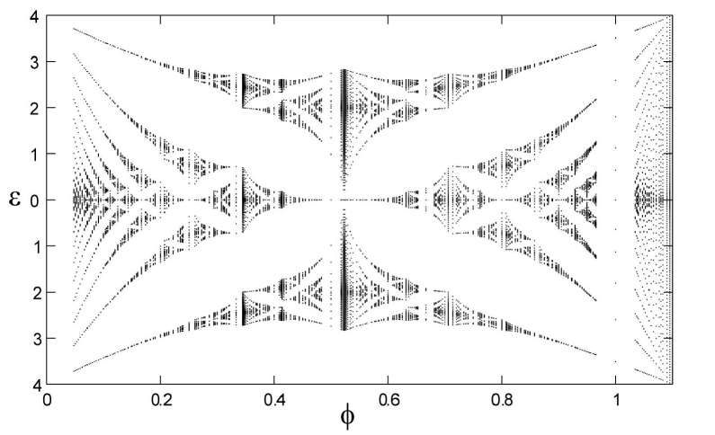
Figure 1: Noncommutative Hofstadter butterfly diagram at $\theta=1/3$ which corresponds to the one period of commutative diagram.

In the commutative case, there are $q$ sub-bands at a rational flux, $p/q$. For small $q$, the band width of each sub-bands are large. In the non-commutative space, most of the same region corresponds to that with an irrational flux. Then the energy spectrum becomes singular, i.e. the number of the sub-bands diverges and the band width is zero. The rational flux in commutative space and the flux $\phi$ in noncommutative space relates

$$\frac{p}{q}=\phi\left(1-\dfrac{\frac{r}{s}\phi}{4}\right).$$ (36)

for a rational $\theta=r/s$, where $r$ and $s$ are mutually prime number. It is easy to show that the quadratic equation

$$qr\phi^{2}-4sq\phi+4sp=0$$ (37)

hardly have rational solution.

For example, we have two wide sub-bands at $1/2$ flux in commutative space. The corresponding value in non-commutative space is $\phi=6-\sqrt{30}$. It is a irrational limit of the external magnetic field. Therefore, no sub-band with a wide band width exists.

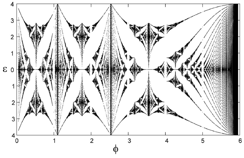
Figure 2: Noncommutative Hofstadter butterfly diagram at $\theta=1/3$.

References

- (1) A. Connes, M.R. Douglas and A. Schwarz, JHEP 02, 003 (1998).
- (2) N. Seiberg and E. Witten, JHEP 09, 032 (1999).
- (3) M.R. Douglas and N.A. Nekrasov, Rev. Mod. Phys. 73, 977 (2001).
- (4) T. Curtright, D. Fairlie and C. Zachos, Phys. Rev. D 58, 025002 (1998).
- (5) C. Duval and P.A. Horvathy, Phys. Lett. B 479, 284 (2000).
- (6) V.P. Nair and A.P. Polychronakos, Phys. Lett. B 505, 267 (2001).
- (7) O. Dayi and A. Jellal, J .Math. Phys. 43, 4592 (2002); ibid. 45, 827 (2004).
- (8) J. Gamboa, M. Loewe, J.C. Rojas, hep-th/0101081; J. Gamboa, M. Loewe, F. Mendez, J.C. Rojas, Mod. Phys. Lett. A 16, 2075 (2001).
- (9) M. Chaichian, P. Presnajder, M.M. Sheikh-Jbbari and A. Tureanu, Phys. Lett. B 527, 149 (2002).
- (10) P.G. Harper, Proc. Phys. Soc. London Sect. A 68, 874 (1955).
- (11) G.H. Wannier, J. Math. Phys. 21, 2844 (1980).
- (12) D.R. Hofstadter, Phys. Rev. B 14, 2239 (1976).
- (13) For a review, see H. Hiramoto and M. Kohmoto, Int. J. Mod. Phys. B 6, 281 (1992).
- (14) D.J. Thouless, Phys. Rev. B 28, 4272 (1983).
- (15) D.J. Thouless, M. Kohmoto, P. Nightingale and M. den Nijs, Phys. Rev. Lett. 49, 405 (1982).
- (16) Q. Niu, D.J. Thouless and Y.S. Wu, Phys. Rev. B 31, 3372 (1985).
- (17) For example, see Y. Hatsugai, M. Kohmoto and Y. Wu, Phys. Rev. B 53, 9697 (1996); Y. Hatsugai, J. Phys.: Condens. Matter 9, 2507 (1997).
- (18) H. Takahashi and M. Yamanaka, to be published