UPR-1154-T
LBNL-60486
hep-th/0606118

Four Dimensional Black Hole Microstates:
From D-branes to Spacetime Foam

Vijay Balasubramanian^,a, Eric G. Gimon^,b,c and Thomas S. Levi^,a

^a David Rittenhouse Laboratories, University of Pennsylvania, Philadelphia, PA 19104, USA.

^b Department of Physics, University of California, Berkeley, CA 94720, USA.

^c Theoretical Physics Group, LBNL, Berkeley, CA 94720, USA.

We propose that every supersymmetric four dimensional black hole of finite area can be split up into microstates made up of primitive half-BPS “atoms”. The mutual non-locality of the charges of these “atoms” binds the state together. In support of this proposal, we display a class of smooth, horizon-free, four dimensional supergravity solutions carrying the charges of black holes, with multiple centers each carrying the charge of a half-BPS state. At vanishing string coupling the solutions collapse to a bound system of intersecting D-branes. At weak coupling the system expands into the non-compact directions forming a topologically complex geometry. At strong coupling, a new dimension opens up, and the solutions form a “foam” of spheres threaded by flux in M-theory. We propose that this transverse growth of the underlying bound state of constitutent branes is responsible for the emergence of black hole horizons for coarse-grained observables. As such, it suggests the link between the D-brane and “spacetime foam” approaches to black hole entropy.

1 Introduction

String theory has suggested two different pictures of the microstates underlying the entropy of black holes. The first, due originally to [1, 2], describes the underlying states as fluctuations of complicated bound states of string solitons. These analyses typically apply at very weak coupling, when there is no macroscopic horizon. A second picture (see the reviews [3, 4]) suggests that, at least in situations with sufficient supersymmetry, some of the underlying microstates can appear directly in gravity as a sort of “spacetime foam” [3, 4, 5, 6, 7], the details of which are invisible to almost all probes [8]. In this picture, the black hole with a horizon is simply the effective semiclassical description of the underlying “foam”. The present paper suggests how these two pictures are connected for four dimensional black holes – as the string coupling grows, D-brane bound states that form black hole microstates grow a transverse size, leading to a gravitational description as a topologically complex “spacetime foam”.

We provide evidence for this picture by constructing a large class of smooth, horizon-free, four dimensional supergravity solutions that have the charges of macroscopic black holes. Our construction proceeds by compactifying the five-dimensional (M-theory on $T^{6}$) solutions of [6, 5]. Typical geometries contain multiple centers, each carrying the charge of a 1/2-BPS state. The geometries are characterized by a region of complex topology containing a “foam” of spheres threaded by flux. This leads to a proposal: Every supersymmetric four dimensional black hole can be split up into microstates made of 1/2-BPS “atoms”. The mutual nonlocality of the charges of these “atoms” binds the solution together.

The geometric structures in our solutions scale as the string coupling is changed. As the string coupling $g_{s}$ decreases, the region of complex topology shrinks until it is best interpreted in terms of wrapped D-branes whose separations are proportional to $g_{s}$. As $g_{s}$ decreases further, the states can be described in the low-energy quiver gauge theory of a system of intersecting D-branes, following Denef [13]. Thus we arrive at a picture where quantum gravity microstates associated to a spacetime with fixed asymptotic quantized charges go through various transitions as the coupling is changed. Every microstate begins life at $g_{s}=0$ as a ground state of an intersecting D-brane system. As we increase the coupling, the microstate makes a transition from a quiver gauge theory in the Higgs phase, to one in the Coulomb phase. As we further increase the coupling, a closed string picture becomes appropriate and, for states having a classical limit, we obtain the four dimensional solutions described in this paper. Still further increasing the coupling to large $g_{s}$ opens up the eleventh dimension and we find a “spacetime foam” in M-theory of two-cycles threaded by flux [6, 5]. A similar flow from D-branes to “spacetime foam” has been noted in the topological string [14].

2 Review of five dimensional solutions

Here we review the candidate smooth, horizon-free microstates for black holes and black rings in five dimensions that were derived in [6, 5]. We will find candidate microstate solutions for four dimensional, finite area black holes by compactifying these geometries.

Basic setup:

M-theory reduced to five dimensions on a 6-torus has 1/8-BPS solutions that only carry membrane charges. The general ansatz for such solutions was given in [15] following [16, 17]. The five dimensional non-compact space is written as time fibered over a pseudo-hyperkahler base space ($HK$) which we require here to have a $U(1)$ symmetry. The metric takes the form:

$$ds^{2}_{11}=-(Z_{1}Z_{2}Z_{3})^{-2/3}(dt+k)^{2}+(Z_{1}Z_{2}Z_{3})^{1/3}ds^{2}_{HK}+ds^{2}_{T^{6}},$$ (2.1)

where

$$ds^{2}_{HK}=H^{-1}\sigma^{2}+H(dr^{2}+r^{2}d\theta^{2}+r^{2}\sin^{2}\theta d\phi^{2})\,.$$ (2.2)

Here $k$ is a 1-form on the hyperkahler base. $H$ is a harmonic function on the flat ${\bf R}^{3}$ parametrized by $(r,\theta,\phi)$ with poles having integer residues. Likewise, $\sigma$ is a one-form on ${\bf R}^{3}$ ($\sigma=d\tau+f_{a}dx^{a}$ where $\tau$ has period $4\pi$) satisfying

$$\star_{3}d\sigma=dH\,.$$ (2.3)

The Hodge dual $\star_{3}$ acts in the flat ${\bf R}^{3}$ only. The metric on the torus is

$$ds^{2}_{T^{6}} = (Z_{1}Z_{2}Z_{3})^{1/3}\left(Z_{1}^{-1}(dz_{1}^{2}+dz_{2}^{2})+Z_{2}^{-1}(dz_{3}^{2}+dz_{4}^{2})+Z_{3}^{-1}(dz_{5}^{2}+dz_{6}^{2})\right).$$ (2.4)

The $Z_{i}$’s are functions on the hyperkahler base space, and the associated 2-tori have volumes $V_{i}$. The gauge field takes the form:

$$C_{(3)} = -(dt+k)\wedge\left(Z_{1}^{-1}\,dz_{1}\wedge dz_{2}+Z_{2}^{-1}\,dz_{3}\wedge dz_{4}+Z_{3}^{-1}\,dz_{5}\wedge dz_{6}\right)$$ (2.5)

$$+2\,a^{1}\wedge dz_{1}\wedge dz_{2}+2\,a^{2}\wedge dz_{3}\wedge dz_{4}+2\,a^{3}\wedge dz_{5}\wedge dz_{6},$$

where the $a^{i}$ are one-forms on the base space. After reduction on $T^{6}$ the C-field leads to three separate $U(1)$ bundles, with connections ${\cal A}^{i}=-(dt+k)Z^{-1}_{i}+2\,a^{i}$, on the five-dimensional total space. Defining $G^{i}=da^{i},$ [15] show that the equations of motion reduce to the three conditions (here the Hodge operator refers only to the base space $H\!K$):

$$G^{i}=\star G^{i},\qquad d\!\star\!dZ_{i}=2s_{ijk}\,G^{j}\wedge G^{k},\qquad dk+\star dk=2\,G^{i}Z_{i},$$ (2.6)

where we define the symmetric tensor $s^{ijk}=|\epsilon^{ijk}|$.

Solution:

This system of equations can be completely solved in terms of seven harmonic functions in addition to $H$, defined using variables $r_{p}=|\vec{x}-\vec{x_{p}}|$, where $\vec{x}$ is a coordinate in the ${\bf R}^{3}$ appearing in (2.2):

$$H=\sum_{p\,=1}^{N}{n_{p}\over r_{p}},\qquad M_{i}=1+\sum_{p\,=1}^{N}{Q^{p}_{i}\over 4r_{p}},\qquad K=l_{0}+\sum_{p\,=1}^{N}{l_{p}\over r_{p}},\qquad h^{i}=\sum_{p\,=1}^{N}{d_{p}^{i}\over 4r_{p}}.$$ (2.7)

To achieve an asymptotically flat metric, we require the NUT charge

$$n_{T}=\sum_{p}n_{p}$$ (2.8)

to equal $1$. (The standard radial coordinate for the asymptotic ${\bf R}^{4}$ is $R=2\sqrt{r}$.) At each point $p$, the $Q_{i}^{p}$ measure the membrane charges, $n_{p}$ sets the Kaluza-Klein monopole charge, $l_{p}$ measures the angular momentum associated to the $U(1)$ isometry. The $d_{p}^{i}$ make contributions to the total 5-brane dipole moment of the solution. In terms of these functions, the equations of motion can be solved, giving:

$$Z_{i} = M_{i}+2s_{ijk}h^{j}h^{k}/H,\qquad a^{i}=(h^{i}/H)\,\sigma+a^{i}_{a}dx^{a},\qquad d(a_{ia}dx^{a})=-\star_{3}dh^{i},$$

$$k = k_{0}\,\sigma+k_{a}\,dx^{a},\qquad k_{0}=K+8H^{-2}\,h^{1}\,h^{2}\,h^{3}+H^{-1}\,M_{i}\,h^{i}$$

$$d(k_{a}dx^{a}) = H\star_{3}dK-K\,\star_{3}dH+h^{i}\,\star_{3}dM_{i}-M_{i}\,\star_{3}dh^{i}$$ (2.9)

Requiring the absence of pathologies in these solutions constrains the parameters in various ways.

Constraints:

The requirement of smoothness (no curvature singularities) constrains the charges of the harmonic functions:

$$Q^{p}_{i}=-s_{ijk}{d^{j}_{p}d^{k}_{p}\over 2n_{p}},\qquad l_{p}={d^{1}_{p}d^{2}_{p}d^{3}_{p}\over 16n_{p}^{2}},\qquad l_{0}=-\sum_{i}{\sum_{p}d^{i}_{p}\over 4n_{T}}\equiv-\sum_{i}{s^{i}\over 4n_{T}}.$$ (2.10)

It is useful to define

$$\tilde{\lambda}_{p}^{i}=(d_{p}^{i}/n_{p}-s^{i}/n_{T}),\qquad\Gamma_{pq}={\prod_{i}(n_{p}d_{q}^{i}-n_{q}d^{i}_{p})\over n_{p}^{2}n_{q}^{2}}\,,$$ (2.11)

in terms of which the closure condition for $d(k_{a}dx^{a})$, which makes $k_{a}dx^{a}$ a globally well defined one-form, becomes

$$4\sum_{i}n_{p}\tilde{\lambda}_{p}^{i}+\sum_{q=1}^{N}{\Gamma_{pq}\over r_{pq}}=0,\qquad p=1...(N-1).$$ (2.12)

where $r_{pq}=|\vec{x}_{p}-\vec{x}_{q}|$. While (2.10) constrains the parameters of a smooth solution, (2.12) determines the relative separations of the poles in (2.7). For a fixed set of charges, there are $N-1$ nonlinear equations relating $3N-3$ variables (after we fix the center of mass), so if a solution exists for a given set of charges satisfying (2.10), the locations of the poles supporting the charges will typically be a function of $2N-2$ moduli. We can set three more free parameters (although these are not completely independent of the charges) by specifying the angular momentum $J_{L}$ defined below and its orientation. Finally, the absence of closed timelike curves and horizons in the solution requires that

$$(Z_{1}Z_{2}Z_{3}H-k_{0}^{2}H^{2}-g^{ab}_{{\bf R}^{3}}k_{a}k_{b})>0$$ (2.13)

must be satisfied everywhere. This condition also guarantees smoothness on the $H=0$ surface and that the metric has constant signature. It is possible that (2.13) is implied by (2.12) via some kind of gradient flow argument, but this is not immediately evident.

Charges:

The total membrane charges and angular momenta of the solution are:

$$Q_{i} = -{1\over 2}\sum_{p\,=1}^{N}n_{p}s_{ijk}\tilde{\lambda}^{j}_{p}\tilde{\lambda}^{k}_{p},\qquad J_{R}=\sum_{p\,=1}^{N}n_{p}\tilde{\lambda}_{p}^{1}\tilde{\lambda}_{p}^{2}\tilde{\lambda}_{p}^{3},$$ (2.14)

$$\qquad J_{L} = 4|\sum_{p\,=1}^{N}\sum_{i}n_{p}\tilde{\lambda}_{p}^{i}\vec{x}_{p}|\;=\;{1\over 2}\Big{|}\sum_{pq}\Gamma_{pq}{\vec{x}_{p}-\vec{x}_{q}\over|\vec{x}_{p}-\vec{x}_{q}|}\Big{|}.$$ (2.15)

The solution also carries a net 5-brane dipole moment. Finally, the absence of Dirac strings in the $C$-field requires integral quantization conditions:

$$n_{p},\;\;{\pi\Gamma_{pq}\over 4G^{(5)}_{N}}\in{\bf Z},\qquad d_{p}^{i}=m^{i}_{p}/e^{i},\qquad m^{i}_{p}\in{\bf Z},$$ (2.16)

with constants

$$e^{i}={V_{i}\over(2\pi)^{2}\ell_{P}^{3}},\qquad\prod_{i}(e^{i})^{-1}={4G_{5}\over\pi}.$$ (2.17)

Appropriate quantization of the membrane charge and angular momenta also imposes

$$m_{p}^{i}m_{p}^{j}/n_{p}\in{\bf Z},\qquad m_{p}^{1}m_{p}^{2}m_{p}^{3}/n_{p}^{2}\in{\bf Z}\,.$$ (2.18)

3 Reducing to Four Dimensions

Type II string theory compactified on a 6-torus has a spectrum of extremal supersymmetric black holes. The charge vector of these black holes transforms in the 56 representation of the $E_{7(7)}$ duality group. The entropy associated with the black hole horizons is a function of the quartic invariant of $E_{7(7)}$ constructed from the charges (see, e.g., [18, 19]). As a result, to have a finite entropy, these black holes must have at least four charges. Furthermore, a generating solution whose $E_{7(7)}$ orbit traces out the entire 56 dimensional space of extremal black holes must have at least five charges, of which one pair must be electric-magnetic duals [20, 21]. We are interested in finding candidate supergravity microstate solutions for such a generating black hole.

In the previous section we described a class of candidate microstates for five dimensional black rings and black holes in M-theory having a $U(1)$ isometry. These solutions carry three M2-brane charges and momentum along the $U(1)$ direction. Upon compactifying along this direction, these charges give rise to D2-branes and D0-branes in IIA string theory. To carry out the reduction to four dimensions we modify the solution in the previous section so that the $U(1)$ direction approaches a finite size at infinity. M5-branes can wrap on this circle leading to three D4-brane charges in IIA string theory. In addition, the now arbitrary NUT charge in the solution leads to D6-brane charge, giving in total eight charges. A similar procedure, of placing five dimensional solutions in Taub-Nut, has been used to relate five dimensional black holes and rings to four dimensional black holes [22, 23]. All of these charges arise from wrapped D6-branes with fluxes. Since D2s and D4s as well as D0s and D6s are electric-magnetic duals, these configurations also have the charges necessary for them to be smooth microstates associated to a finite area, extremal 1/8-BPS black hole.

3.1 Introducing Taub-NUT

The five dimensional solution in Sec. 2 has a direction of $U(1)$ isometry. In order to reduce on this circle it must approach a finite size at infinity We can accomplish this by adding a constant to $H$ which effectively places the M2-branes in a Taub-NUT background:

$$H\to H+\delta H~{}~{}~{};~{}~{}~{}\delta H={4\over L^{2}}.$$ (3.1)

The asymptotic circumference of the circle is $2\pi L$. We allow the NUT charge (2.8) to be arbitrary, the full solution (2.1,2.5) can then be interpreted in terms of M2-branes in a Taub-NUT background.

In order to ensure gauge invariance under transformations of the C-field it is necessary to also add constants $\delta h^{i}$ to the $h^{i}$ harmonic functions. In terms of these shifts it is convenient to define

$$\lambda_{p}^{i}={d^{i}_{p}\over n_{p}}-{4\delta h^{i}\over\delta H}={d^{i}_{p}\over n_{p}}-L^{2}\,\delta h^{i},$$ (3.2)

and to re-write the the constant part of $K$ (making sure there are no CTCs at infinity by bounding the last term) as:

$$\delta K={L^{4}\over 4}\prod_{i}\delta h^{i}-{L^{2}\over 4}\sum_{i}\delta h^{i}+{L\over 2}\sin\alpha$$ (3.3)

To achieve a standard locally flat metric at infinity, we set the constant part of $M_{i}$ to

$$\delta M_{i}=1-2s_{ijk}{\delta h^{j}\delta h^{k}\over\delta H}.$$ (3.4)

We can also set $k_{0}\to 0$ at infinity by setting $\alpha=0$. This is not necessary for getting a flat asymptotic metric, as we can always set this constant to zero by shifting the coordinate $\tau$ by a function of $t$. This adds another layer of unnecessary complication (see Appendix B for the full construction), and without loss of generality we will assume that $\alpha=0$. We do require, however, that the derivative of the angular momentum,

$$dk=d(k_{0}f_{a}dx^{a})+d(k_{a}dx^{a})$$ (3.5)

falls off at infinity. This yields the constraint

$$\sum_{p}\Psi_{p}=0,\qquad\Psi_{p}=\sum_{i}n_{p}\lambda^{i}_{p}-{1\over L^{2}n_{p}^{2}}\prod_{i}n_{p}\lambda^{i}_{p}.$$ (3.6)

In lifting back to five noncompact dimensions the shifts $\delta h^{i}$ and $\delta H$ are set to zero so that subleading terms in $h^{i}$ and $H$ determine the ratio

$$\lim_{r\to\infty}{4h^{i}\over H}\to{s^{i}\over n_{T}}.$$ (3.7)

Thus, in the decompactification limit (3.6) is tautological. The integrability condition on $k_{a}dx^{a}$ becomes

$$4\Psi_{p}+\sum_{q}{\Gamma_{pq}\over r_{pq}}=0,\qquad p=1...N.$$ (3.8)

(Compare with (2.12) in the $L\to\infty$ decompactification limit.) Only $N-1$ of these are independent if we take (3.6) into account. Specifying the angular momentum $\vec{J}_{L}$ provides three more constraints ($J_{R}$ will be related to the $D0$-charge):

$$J_{R} = \sum_{p}n_{p}\prod_{i}\lambda^{i}_{p}$$ (3.9)

$$\vec{J}_{L} = -4\sum_{p}\Psi_{p}\,\vec{x}_{p}={1\over 2}\,\sum_{pq}\Gamma_{pq}\hat{r}_{pq}.$$ (3.10)

The second equality for $\vec{J_{L}}$ used the constraint equation (3.8).

3.2 Reduction to IIA

We obtain a solution to IIA string theory by reducing along $y=(L/2)\,\tau$ ($y$ has period $2\pi L$) in terms of dimensionless versions of the eight harmonic functions ($M_{i}$ is already dimensionless)

$$M_{0}=-HL^{2}/4,\qquad K^{0}=4K/L,\qquad K^{i}=Lh^{i}.$$ (3.11)

The reduction gives the metric

$$ds^{2}_{IIA}=-J_{4}^{-1/2}(dt+k_{a}dx^{a})^{2}+J_{4}^{1/2}\Big{(}ds^{2}_{{\bf R}^{3}}+\sum_{i=1}^{3}(-Z_{i}M_{0})^{-1}ds^{2}_{T_{i}}\Big{)}\,.$$ (3.12)

The radius of the compactification circle is related to the string length and coupling as

$$L=g_{s}l_{s}$$ (3.13)

The $T_{i}$ are flat 2-tori with volume forms $dV_{i}$. The dilaton and form fields are

$$e^{2\Phi}=(J_{4})^{3/2}(-Z_{1}Z_{2}Z_{3}M_{0}^{3})^{-1},\qquad B_{2}=-\Big{(}{K^{i}\over M_{0}}+{2k_{0}\over L\,Z_{i}}\Big{)}dV_{i}$$ (3.14)

$$C_{1}={L\over 2}f_{a}dx^{a}-{2M_{0}^{2}k_{0}\over LJ_{4}}(dt+k_{a}dx^{a})$$ (3.15)

$$C_{3}=\Big{[}-Z_{i}^{-1}(dt+k_{a}dx^{a})+2\vec{a}_{i}-\Big{(}{K^{i}\over M_{0}}+{2k_{0}\over L\,Z_{i}}\Big{)}{L\over 2}f_{a}dx^{a}\Big{]}\wedge dV_{i}.$$ (3.16)

$J_{4}$ is the quartic invariant of $E_{7(7)}$ constructed from the eight harmonic functions connected to four electric and magnetic “charges” [24]

$$J_{4} = {L^{2}\over 4}\left((Z_{1}Z_{2}Z_{3})H-k_{0}^{2}H^{2}\right)$$

$$= M_{0}K^{0}(M_{i}K^{i})+M_{1}K^{1}(M_{2}K^{2}+M_{3}K^{3})+M_{2}K^{2}M_{3}K^{3}$$

$$- {1\over 4}(M_{\mu}K^{\mu})^{2}-M_{0}M_{1}M_{2}M_{3}-K^{0}K^{1}K^{2}K^{3},\qquad\mu\in 0\ldots 3$$ (3.18)

We have introduced a new radial variable $\rho=2r/L$ so that the metric on the ${\bf R}^{3}$ piece takes the standard flat form.

For the further reduction on the $T_{i}$ to four dimensions it is useful to define a shifted 3-form field that is invariant under shifts of coordinates in the $y$ circle and the three 2-tori.

$$C_{3}^{\prime}=C_{3}-B_{2}\wedge C_{1}=\Big{(}{-M_{0}\over J_{4}}(2K^{i}k_{0}/L-s^{ijk}\,Z_{j}Z_{k}/2)(dt+k_{a}dx^{a})+2\vec{a}_{i}\Big{)}\wedge dV_{i}\,.$$ (3.19)

The quantized $D$-brane charges are

$$Q_{0}^{D6}={L\over 2}\,\sum_{p}(-n_{p})={g_{s}l_{s}\over 2}\,N_{6}, Q_{i}^{D2}=-{1\over 2L}\,\sum_{p}s_{ijk}{d_{p}^{j}d_{p}^{k}\over 2n_{p}}=-{4G_{4}\,V_{i}\over 4\pi^{2}g_{s}l_{s}^{3}}N_{i\,2},$$

$$Q^{0}_{D0}={1\over 2L^{2}}\,\sum_{p}{d_{p}^{1}d_{p}^{2}d_{p}^{3}\over n_{p}^{2}}={4G_{4}\over g_{s}l_{s}}\,N_{0}, Q^{i}_{D4}={1\over 2}\,\sum_{p}d_{p}^{i}=2\pi^{2}\,{g_{s}l_{s}^{3}\over V_{i}}N_{4}^{i}\,.$$ (3.20)

In our conventions the D0 and D4-branes are magnetic objects while the D2 and D6-branes are electric. While the charges defined here are quantized, they are not invariant under large gauge transformations of the $B$-field because of Chern-Simons terms in the supergravity Lagrangian. (See [25] for the difference between quantized and gauge-invariant charges.) In the four dimensional theory we will interpret large gauge transformations of the $B$-field as $SU(8)$ transformations inside $E_{7(7)}$. Our sign conventions are consistent with the Hodge dual relations $F_{6}=*F_{4},F_{2}=*F_{8}$. Each of these charges is written as a sum over points $p$, and at each point we can interpret the charges as arising from a D6-brane with fluxes on it.

3.3 Reduction to four dimensions and special geometry

$E_{7}$ structure:

Upon reduction to four dimensions, we obtain solutions to ${\cal N}=8$ supergravity [26]. This theory has an $E_{7(7)}$ duality group. The three D2-brane charges and the D6-brane charge transform in an electric ${\bf 28}$ representation of the maximal compact subroup $SU(8)/{\bf Z}_{2}$, while the three D4-brane charges and the D0-brane transform in a magnetic ${\bf 28}$. Together, these charges transform in the ${\bf 56}$ representation of $E_{7(7)}$ ; we can write combined charge vectors with eight of these charges turned on:

$$\Gamma_{p} = \Big{(}Q_{0}^{p},\;Q_{i}^{p},\;Q^{0}_{p},\;Q^{i}_{p}\Big{)}=\Big{(}{-L\over 2}n_{p},\;\;{-1\over 4L}s_{ijk}{d_{p}^{j}d_{p}^{k}\over n_{p}},\;\;{1\over 2L^{2}}{d^{1}_{p}d^{2}_{p}d^{3}_{p}\over n_{p}^{2}},\;\;{1\over 2}d^{i}_{p}\Big{)}.$$ (3.21)

$$\Gamma = \sum_{p}\Gamma_{p}=\Big{(}Q_{0},\;Q_{i},\;Q^{0},\;Q^{i}\Big{)}$$ (3.22)

(To avoid clutter we leave out the D0, D2 etc. notation in (3.20).) The symplectic $E_{7}$ invariant constructed from these charges is

$$<\Gamma_{p},\Gamma_{q}>\,=\,{1\over 2}\left(Q^{0}_{p}Q_{0}^{q}-Q^{0}_{q}Q_{0}^{p}+Q^{i}_{p}Q_{i}^{q}-Q^{i}_{q}Q_{i}^{p}\right)={\Gamma_{pq}\over 8L}=G^{(4)}_{N}\gamma_{pq},\;(\gamma_{pq}\in{\bf Z}).$$ (3.23)

Similarly, we can think of our eight harmonic functions as part of a single harmonic function valued in the ${\bf 56}$ of $E_{7(7)}$ written as ($\Gamma_{\infty}$ denotes the constant terms):

$${\cal H}=\Big{(}M_{0},\;M_{i},\;K^{0},\;K^{i}\Big{)}=\Gamma_{\infty}+\sum_{p}{\Gamma_{p}\over\rho_{p}}\,.$$ (3.24)

Then the 1-form in (2) which gives rise to the angular momentum in the solution satisfies

$$\star_{3}d(k_{a}dx^{a})=\star_{3}d\vec{k}=\,<d{\cal H},{\cal H}>.$$ (3.25)

At this juncture, we see that the reduction of our M-theory solutions down to ${\cal N}=8$ supergravity in four dimensions yields a framework similar to the ${\cal N}=2$ setup in [27, 28, 29]. In fact, our theory with eight vector fields and six scalars corresponds to a truncation of the ${\cal N}=8$ theory to the famous STU ${\cal N}=2$ model [30, 35] which corresponds to the symmetric coset space $[SL(2,R)/U(1)]^{3}$.

Explicit solution and special geometry:

The four-dimensional metric is the obvious truncation of (3.12)

$$ds^{2}_{4}=-J_{4}^{-1/2}(dt+k_{a}\,dx^{a})^{2}+J_{4}^{1/2}ds^{2}_{{\bf R}^{3}}$$ (3.26)

The four dimensional dilaton is constant, because the volume of the three 2-tori in (3.12) cancels the spatial dependence of the ten dimensional dilaton in (3.14). The solution has three complex scalar fields coming from the complexified Kahler moduli of the three $T_{i}$ ($\phi^{i}=i{\rm Vol}^{i}+B_{2}^{i}$). In terms of the explicit ten dimensional solution (3.12,3.14), the scalars are

$$\phi^{i} = i{-2J_{4}^{1/2}\over 2M_{0}M_{i}-s_{ijk}\,K^{j}K^{k}}-\left({2M_{i}K^{i}+M_{0}K^{0}-\sum_{j}M_{j}K^{j}\over 2M_{0}M_{i}-s_{ijk}\,K^{j}K^{k}}\right),$$ (3.27)

$$= \left({\partial J_{4}^{1\over 2}\over\partial M_{i}}-{i\over 2}K^{i}\right)\Bigg{/}\left({\partial J_{4}^{1\over 2}\over\partial K^{0}}+{i\over 2}M_{0}\right)\,.$$ (3.28)

In the first line there is no sum on $i$. In the second line the scalars have been written entirely in terms of the $J_{4}$ invariant and individual harmonic functions transforming in an eight-dimensional subspace of the ${\bf 56}$ of $E_{7(7)}$. These six scalars are part of the ${\bf 70}$ scalars of the $E_{7(7)}/SU(8)$ coset. Finally, the $C_{3}$ field and $C_{1}$ field give $3+1$ vectors (the above three vector multiplets plus the graviphoton) which transform, along with their duals, in the same subspace of the ${\bf 56}$ representation as the harmonic functions. The potentials and their duals can be summarized in a single vector as

$${\bf{\cal\vec{A}}}=\Big{(}\vec{{\cal A}}_{0},\;\vec{{\cal A}}_{i},\;\vec{{\cal A}}^{0},\;\vec{{\cal A}}^{i}\Big{)},$$ (3.29)

with components from reducing $C^{\prime}_{3}$ and $C_{1}$:

$$\vec{{\cal A}}^{i}=-{1\over J_{4}}{\partial J_{4}\over\partial M_{i}}(dt+k_{a}dx^{a})+2\vec{a}^{i},\qquad\vec{{\cal A}}_{0}=+{1\over J_{4}}{\partial J_{4}\over\partial K^{0}}(dt+k_{a}dx^{a})+2\vec{a}_{0},$$ (3.30)

and their duals:

$$\vec{{\cal A}}_{i}=+{1\over J_{4}}{\partial J_{4}\over\partial K^{i}}(dt+k_{a}dx^{a})+2\vec{a}_{i},\qquad\vec{{\cal A}}^{0}=-{1\over J_{4}}{\partial J_{4}\over\partial M_{0}}(dt+k_{a}dx^{a})+2\vec{a}^{0}.$$ (3.31)

The magnetic parts of these potentials are concisely written as:

$$d\vec{a}=\Big{(}d\vec{a}_{0},\;d\vec{a}_{i},\;d\vec{a}^{0},\;d\vec{a}^{i}\Big{)}=-\star_{3}d{\cal H}.$$ (3.32)

$E_{7(7)}$ and more general solutions:

The solutions presented above have four vector fields and six scalars, corresponding to a truncation of the the full ${\cal N}=8$ theory to the ${\cal N}=2$ STU model [35]. More generic four dimensional solutions with arbitrary charges can be obtained by generalizing the above, allowing the harmonic functions (3.24) as well as the indivdual charge vectors (3.21) to occupy the full ${\bf 56}$ of $E_{7(7)}$. Typically, however, the most general configurations of this type will break supersymmetry. Since we are interested in 1/8-BPS states, our charges always need to line up with a preferred ${\cal N}=2$ subalgebra, corresponding to the reduction of $E_{7(7)}$ to $SO^{*}(12)\times SU(2)_{R}$ (for more details see [31, 32, 33]). For such configurations, the appropriate charge subspace for supersymmetry yields vectors (and harmonic functions) which transform in the real ${\bf 32}$ spinor representation of $SO^{*}(12)$, accompanied by thirty non-trivial scalars. The remaining forty scalars of the ${\cal N}=8$ theory appear as hypermultiplet scalars with respect to the $N=2$ truncation, parameterizing the coset $E_{6(2)}/SU(2)_{R}\times SU(6)$. Their values stay fixed throughout our solutions, and are generally constrained by the alignment of the subgroup $SO^{*}(12)\times SU(2)_{R}$ inside $E_{7(7)}$.

Generalized constraint and coarse graining:

For general charge vectors $\Gamma_{p}$ the constraint equation (3.8) can be appropriately generalized by requiring integrability (3.25) as before. Then, in terms of a symplectic product of the charges and the asymptotic values of the harmonic functions (3.24),

$$<\Gamma_{p},\Gamma_{\infty}>+\sum_{q}{<\Gamma_{p},\Gamma_{q}>\over\rho_{pq}}=0.$$ (3.33)

The first term automatically provides an expression for the $\Psi_{p}$’s and summing these equations provides the first of the two constraints on $\Gamma_{\infty}$,

$$<\Gamma,\Gamma_{\infty}>=0,\qquad I_{4}\left(\Gamma_{\infty}\right)=1,$$ (3.34)

which tell us that the asymptotic scalars sit in the appropriate coset.

In the form above, the constraint equation also gives us an insight into the behavior of the solution if we “coarse-grain” over a collection of charges by collecting them into a single pole. For example, let us partition our poles into sets ${\cal P}$ containing poles seperated by distances much smaller than some reference scale, $\Lambda$. Then we can define a coarse-grained solution by assigning the total charge of each cluster ${\cal P}$ to the mean location of the poles in the cluster:

$$\Gamma_{\cal P}=\sum_{p\in{\cal P}}\Gamma_{p},\qquad\vec{x}_{\cal P}\sim<\vec{x}_{p}>.$$ (3.35)

The constraints on the coarsened solution are then:

$$<\Gamma_{\cal P},\Gamma_{\infty}>+\sum_{\cal Q}{<\Gamma_{\cal P},\Gamma_{\cal Q}>\over\rho_{{\cal PQ}}}\;<<\;\Lambda.$$ (3.36)

An important feature of this coarse-graining is that if a cluster of poles ${\cal P}$ has the property that $<\Gamma_{\cal P},\Gamma_{\infty}>=0$, then this cluster can be placed at an infinite distance from the rest of the poles, distinguishing our supergravity solution as one generated by at least two separate bound states.

The maximally coarse-grained solution replaces the detailed microstate by a solution with a single pole carrying the total charge vector of the spacetime. Below we will show that such single-pole solutions are black holes of the ${\cal N}=8$ supergravity and will in general have a finite horizon area.

3.4 Relation to finite area black holes

We would like to understand how the solutions described above can be seen as candidate microstates for the extremal black holes of ${\cal N}=8$ supergravity. Far away from all the poles, the harmonic function ${\cal H}$ can be well approximated by the single center function

$${\bar{\cal H}}=\Gamma_{\infty}+{\Gamma\over\rho}$$ (3.37)

where $\Gamma$ is the total charge vector defined in (3.22). Plugging this simplified function into our formulism yields a metric with no angular momentum  and

$$J_{4}(\rho)={I_{4}(\Gamma)\rho^{-4}}\,,$$ (3.38)

where $I_{4}(\Gamma)$ comes from expression (3.2) for $J_{4}$ after we substitute in the appropriate charge for each harmonic function. If $I_{4}(\Gamma)>0$, this is simply the spherically symmetric metric of a 1/8-BPS black hole with total charge vector $\Gamma$ and horizon area given by

$$A=2\pi\sqrt{I_{4}(\Gamma)}\,.$$ (3.39)

If $I_{4}(\Gamma)<0$ (the null case will become clear later), we have taken our coarse-graining procedure too far, and need to retreat back until we only have centers with $I_{4}(\Gamma_{\cal P})\geq 0$. The astute reader can recognize $I_{4}$ as Cartan’s quartic $E_{7}$ invariant [18, 19, 5, 34]. In terms of the antisymmetric central charge matrix $z_{ij}=x_{ij}+iy_{ij}$ of ${\cal N}=8$ supergravity, this invariant is written as

$$4I_{4}={x^{ij}y_{ij}x^{kl}y_{kl}\over 4}-x^{ij}y_{kj}x^{kl}y_{li}-{1\over 96}(\epsilon^{ijklmnop}x_{ij}x_{kl}x_{mn}x_{op}+\epsilon_{ijklmnop}y^{ij}y^{kl}y^{mn}y^{op})\,.$$ (3.40)

Here indices are raised and lowered by $\delta^{i}_{j}$. In our conventions

$$x^{12} = Q^{1}~{}~{}~{};~{}~{}~{}x^{34}=Q^{2}~{}~{}~{};~{}~{}~{}x^{56}=Q^{3}~{}~{}~{};~{}~{}~{}x^{78}=Q^{0}$$ (3.41)

$$y_{12} = Q_{1}~{}~{}~{};~{}~{}~{}y_{34}=Q_{2}~{}~{}~{};~{}~{}~{}y_{56}=Q_{3}~{}~{}~{};~{}~{}~{}y_{78}=Q_{0}$$ (3.42)

For a solution with only the D2 (D4) and D6 (D0) brane charges, the expected horizon area of the associated black hole is

$${\rm D2-D2-D2-D6\ area:}~{}~{}~{}~{}~{}A = 2\pi\sqrt{-Q_{0}\prod_{i}Q_{i}}$$ (3.43)

$${\rm D4-D4-D4-D0\ area:}~{}~{}~{}~{}~{}A = 2\pi\sqrt{-Q^{0}\prod_{i}Q^{i}}$$ (3.44)

The sign under the square root indicates that the D6 (D0) must be appropriately oriented relative to the D2 (D4) branes to preserve supersymmetry [21]. If electric and magnetic dual objects are present, other terms in $I_{4}$ will also contribute. The space of all extremal finite area black holes in ${\cal N}=8$ supergravity can be generated by $E_{7(7)}$ transformations of generating configurations with five charges containing one electric-magnetic pair [31, 21, 19]. An example generating configuration contains three D2-brane, D6-brane and D0-brane charges. Such charge vectors are included in our analysis and thus the solutions described earlier in this section provide candidate microstates for the generating black holes of ${\cal N}=8$ supergravity.

It is interesting to ask whether a charge vector of the form (3.21) associated to a single pole in the solution could have given rise to a finite horizon area by itself. Knowing the leading behavior of the functions $Z_{i},k_{0}$ and $H$ it easy to show that

$$\lim_{\vec{x}\to\vec{x}_{p}}J_{4}\propto\rho_{p}^{-1}\qquad\Rightarrow\qquad I_{4}(\Gamma_{p})=0.$$ (3.45)

We can also check that the invariant $I_{4}(\Gamma_{p})$ vanishes in this case by using the conventions (3.41,3.42) and the single pole charge vector as given in (3.21). Thus, a black hole carrying the charges of a single pole in our solutions (3.21) would have vanishing horizon area and entropy. In fact, the growth of $J_{4}$ near one of our “primitive” poles tells us even more. In ([21]) the authors distinguish four kinds of BPS black holes in ${\cal N}=8$ supergravity. One can find examples for each of these by once again looking at configurations with just D2 and D6-brane charge:

$$D2-D2-D2-D6\neq 0:\;1/8\,{\rm BPS},\,I_{4}>0, J_{4}\propto\rho^{-4},$$ (3.46)

$$D2-D2-D6\neq 0:\;1/8\,{\rm BPS},\,I_{4}=0, J_{4}\propto\rho^{-3},$$

$$D2-D6\neq 0:\;1/4\,{\rm BPS},\,I_{4}=0\,,\partial I_{4}=0, J_{4}\propto\rho^{-2},$$

$$D6\neq 0:\;1/2\,{\rm BPS},\,I_{4}=0,\,\partial I_{4}=0,\,\partial\partial|_{Adj}I_{4}=0, J_{4}\propto\rho^{-1}.$$

The notation with $\partial$’s is impressionistic, see [21] for more detail. Thus, the rate of growth of $J_{4}$ yields a simple U-duality invariant method for determining how much supersymmetry is preserved by a given black hole or pole in a multi-pole configuration.

It has been shown on general grounds that to be associated to a finite horizon area, the charge vector of a black hole in ${\cal N}=8$ supergravity can preserve at most four supercharges – such states, including solutions with general 2-brane and 6-brane charges are 1/8-BPS. By contrast, the classification above tells us that charge vectors of individual poles in our solutions are all 1/2-BPS. Another simple way of seeing this is to note that the charges in (3.21) are consistent with having $-n_{p}$ 6-branes with worldvolume fluxes turned on in the 12, 34, and 56 directions. The Chern-Simons couplings on the brane would then precisely reproduce the 4-brane, 2-brane and 0-brane charges given in (3.21). Such states of 6-branes with fluxes are known to be 1/2-BPS, they are T-dual to IIB 3-branes at angles on a $T^{6}$.

Previous work has shown how certain supersymmetric black holes could be thought of as single center marginal bound states of 1/2 BPS objects later understood to be D-branes [35, 36, 37, 38]. Indeed the four classes of solutions in (3.46) correspond precisely to the four types of axion charges appearing in [35, 36, 37, 38]. In our work, the component 1/2 BPS states are spatially separated and are held together in a true bound state because of their nonzero intersection numbers.

$E_{7(7)}$ transformations of microstates:

In general, we can use an $E_{7(7)}$ transformation to take any finite area 1/8 BPS black hole of ${\cal N}=8$ SUGRA with all ${\bf 56}$ charges to one with only the eight charges of the STU model [31, 35], with scalars in $[SL(2,R)/SO(2)]^{3}$. As we mentioned above, we can further use the three compact $SO(2)$’s of the STU models to eliminate three more of the charges to get, for example, a model with just D2-D2-D2-D6-D0 charges. Recall, however, that the proposed microstates for such a black hole will contain a large number of poles with individual charge vectors. Even if the overall black hole charges fall within the STU sector, the charges of the component poles in the underlying microstates will not be restricted in this way since there is not sufficient symmetry to rotate each pole individually; they will typically all lie in different subspaces of the spinor of $SO^{*}(12)$ [33].

3.5 Summary and Proposal

In this section, we reduced a class of smooth candidate microstate solutions for supersymmetric five dimensional black holes and rings to microstates for four dimensional black holes with eight charges. These spacetimes were written as multi-center solutions in which each center served as a 1/2-BPS “atom” for building up the full configuration. The bound state nature of the overall solution was maintained by the mutual non-locality of the charges which led to constraints on their relative positions. This motivates a conjecture:

Every supersymmetric 4D black hole of finite area, preserving 4 supercharges, can be split up into microstates made of primitive 1/2-BPS “atoms”, each of which preserves 16 supercharges. In order to describe a bound state, these atoms should consist of mutually non-local charges.

The next section provides evidence for this picture.

4 From spacetime foam to D-branes

In [39, 40, 41, 42, 43] the entropy of four dimensional black holes of finite area was accounted for in terms of D-brane bound state degeneracies. The basic strategy was to use D-branes to count the states in the $g_{s}\to 0$ limit and then extrapolate back to stronger coupling using supersymmetry. As such the microstructure of the black hole arose from the many degenerate ground states of the D-branes wrapped on the internal space, in our case $T^{6}$. The picture offered above suggests instead that the entropy of the black hole arises from structure in the non-compact four dimensions of spacetime. This is more along the lines of the proposals of Mathur and collaborators [44, 45, 46]. In this section we demonstrate how these two approaches to black hole entropy could be reconciled. The classical supergravity solutions that we have found flow at weak coupling to systems of intersecting branes of the sort originally used in [39, 40, 41, 42, 43] to count black hole microstates. This suggests that the ground states of such coincident branes at vanishing $g_{s}$ flow at weak $g_{s}$ to the four dimensional supergravity solutions that we have described and at strong $g_{s}$ to a spacetime foam in M-theory. Evidence for this picture exists in the analysis of flows of BPS brane bound states discussed by Denef [13].

4.1 A scaling relation

The locations of the centers in each four dimensional geometry in Sec. 3 are determined by the constraint equation (3.8). We can examine how these solutions change as

$$g_{s}\to\beta g_{s}$$ (4.1)

while we hold the volume of the torus fixed in string units

$${\prod_{i}V_{i}\over l_{s}^{6}}={\rm fixed}\,.$$ (4.2)

The quantized charges of the branes, constructed from the integers $n_{p}$ and $m_{p}^{i}$ (2.16) are held fixed, and thus the physical charges (3.20) scale in powers of $\beta$. Putting everything together, under the rescaling (4.1), the constraint equation (3.8) becomes

$$4\Psi_{p}\beta+\beta^{3}\,\sum_{q}{\Gamma_{pq}\over r_{pq}}=0\,.$$ (4.3)

Thus, given a set of separations $\{r_{pq}\}$ that solve the constraint equation for a string coupling $g_{s}$, the set of separations $\{\beta^{2}r_{pq}\}$ solves the constraints for a coupling $\beta g_{s}$. The physical separations are

$$\rho_{pq}={2r_{pq}\over L}$$ (4.4)

and these scale linearly with $g_{s}$:

$$\rho_{pq}\to\beta\rho_{pq}.$$ (4.5)

In order to continue to satisfy the no-CTC condition (2.13) we must also scale the coordinate $\rho$ as

$$\rho\to\beta\rho.$$ (4.6)

This scaling has far reaching consequences. As we go to weaker coupling, the branes move closer together in string units. At some value of the coupling the branes will move within a string length of each other and the appropriate description is in terms of the open strings on the branes.

To estimate when the open string picture becomes valid, first consider the two-center case. Define the dimensionless quantity

$$\psi_{p}=(g_{s}l_{s})^{-1}\Psi_{p}\ .$$ (4.7)

The branes will be much closer than a string length apart when

$$g_{s}\ll{1\over 32\pi^{6}}{\prod_{i}V_{i}\over l_{s}^{6}}\left|{\psi_{1}\over\gamma_{12}}\right|.$$ (4.8)

When all brane separations are roughly of the same order we can estimate that all pairs of branes are closer than the string length when

$$g_{s}\ll{1\over 32\pi^{6}}{\prod_{i}V_{i}\over l_{s}^{6}}\left|{\psi_{p}\over\gamma_{pq}}\right|~{}~{}~{}~{}\forall\,\psi_{p},\gamma_{pq}\,.$$ (4.9)

For a general bound state, there will always be a value of $g_{s}$ small enough that all branes are separated by distances smaller than the string length. For such small $g_{s}$ the supergravity solutions described in Sec. 3 are better described in terms of open string degrees of freedom coming from the D-branes.

Going the other way, as $g_{s}$ increases, the intervals between the IIA D-branes in the solution increase until, at large coupling the IIA description is no longer valid. At that point we move to an M-theory description with the multi-center D-brane solution replaced by a network of two-cycles (“bubbles”) we call spacetime foam. The new reference length becomes the 11-dimensional Planck length; the size of the asymptotic circle in Planck units now becomes a dimensionless modulus like all the others. Recently, a similar flow from D-branes to “spacetime foam” has been noted in the topological string [14].

4.2 The open string picture

When D-branes are much closer than a string length, an open string description is appropriate. The vacua of the brane system can be analyzed just in terms of the low-energy field theory on the D-branes if the massive string excitations can integrated out. This is the case when all the brane separations are less than $l_{s}$ and when all the charge vectors are sufficiently closely aligned. Taking these conditions to be satisfied, we will describe how the supergravity states in Sec. 3 appear as vacua of a D-brane gauge theory when $g_{s}$ is sufficiently small. In this section, we will set $l_{s}=1$.

First consider a single center with charge vector $\Gamma_{p}=N_{p}\,\hat{\Gamma}_{p}$ where $N_{p}$ is the greatest common divisor of the charges appearing in $\Gamma_{p}$, and $\hat{\Gamma}_{p}$ is thus a primitive charge vector. This represents a stack of $N_{p}$ D-branes wrapping $T^{6}$. When the torus is small (as we take it to be), the low energy physics is obtained by dimensionally reducing the D-brane gauged field theory to a gauged quantum mechanics. Thus the latter has the field content of dimensionally reduced ${\cal N}=4,d=4$, $U(N_{p})$ super-Yang-Mills theory. However, since the interactions between different stacks of branes will only preserve four supercharges, it is convenient to decompose into multiplets of ${\cal N}=4,d=1$ Yang-Mills, obtained via dimensional reduction of an ${\cal N}=1,d=4$ theory. This gives one vector multiplet and three adjoint chiral multiplets. The vector multiplet contains three real, adjoint scalars – these parametrize the positions of the stack of branes in the non-compact space. The three complex adjoints parametrize Wilson lines on the 6-branes (or positions within the torus after T-duality).

In addition, stacks of branes with integer intersection number $\gamma_{pq}\neq 0$ (3.23) give rise to $|\gamma_{pq}|$ chiral fields $\phi_{pq}$ charged in the bifundamental of $U(N_{p})\times U(N_{q})$ [47, 48, 49]. If $\gamma_{pq}=0$, i.e. if the charge vectors $\Gamma_{p}$ and $\Gamma_{q}$ are mutually local, then bifundamentals for these branes only appear in chiral and anti-chiral pairs. There is a Higgs term coupling these bifundamentals to the massless adjoint multiplets on each of the two branes. In a generic bound state, however, mutually local charge vector pairs will occur rarely. Hence we will focus on situations where $\gamma_{pq}\neq 0\,\forall p,q$.

Thus, the low-energy field theory describing the system of branes at small $g_{s}$ is a $d=1,\ {\cal N}=4$ quiver quantum mechanics constructed as follows:

1. For each stack of D6-branes at point $p$ with charge vector $\Gamma_{p}$ we associate a $U(N_{p})$ gauge group and vector multiplet. Here $\Gamma_{p}=N_{p}\,\hat{\Gamma}_{p}$ where $N_{p}$ is the GCD of the charges in $\Gamma_{p}$ and $\hat{\Gamma}_{p}$ is primitive. The three real, adjoint scalars ($\vec{x}$) in the vector multiplet correspond to location in the ${\bf R}^{3}$ transverse to the branes.

2. The number of bifundamental chiral fields $\phi_{pq}$ (transforming in the $(\bar{N_{p}},N_{q})$ of $U(N_{p})\times U(N_{q})$) between branes $p$ and $q$ is given by the intersection number $\gamma_{pq}$.

3. Since each charge vector $\Gamma_{p}$ corresponds to a 1/2-BPS state, we will also get at each node the remainder of an ${\cal N}=4$ vector multiplet: three adjoint chiral multiplets. These will mostly play a spectator role in our considerations.

Figure 1: A sample quiver with two nodes.

The general Lagrangian for the vector multiplet, the bifundamental chiral multiplet and their couplings is given in Appendix C of [13]. The terms arising from the additional chiral adjoints can be determined by dimensional reduction of the ${\cal N}=4,d=4$ Lagrangian. For determining the vacua and phases of the theory, we need to know how these additional fields contribute to the D-term and F-term equations and to the masses of the bifundamentals. The FI-term in the Lagrangian takes the form [13]

$$L_{FI}=\sum_{p}{\cal F}_{p}\,{\rm Tr}D_{p}$$ (4.10)

where $D_{p}$ is the auxiliary adjoint field in the $U(N_{p})$ vector multiplet. ${\cal F}_{p}$ is linear in the charges and depends on closed string field values. It only couples to the D-term for the diagonal $U(1)$ of $U(N_{p})$. This is consistent with the notion that if we just slightly separate our stack into two stacks, $U(N_{p})\to U(N_{p_{1}})\times U(N_{p_{2}})$, then ${\cal F}_{p}={\cal F}_{p_{1}}={\cal F}_{p_{2}}$.

Since the adjoint chirals are neutral under the diagonal center-of-mass $U(1)$ they cannot couple to the corresponding D-term and hence to the D-term equation which will most interest us; they only contribute to the other $N_{p}-1$ equations coming from the $SU(N_{p})$ D-terms. What is more, up to at least quadratic order, the adjoint scalars do not have Higgs couplings to chiral bifundamentals which are not paired to anti-chiral ones. To see this, consider a pair of branes with bifundamentals running between them. The pair can be T-dualized to give two 3-branes at angles in IIB string theory. In this context, the expectation values of the adjoint scalars in the quantum mechanics Lagrangian parameterize the positions of the 3-branes on $T^{6}$ and the Wilson lines in the branes. Neither of these affect either the number of intersections between the branes, or the spectrum of strings localized at the intersection points. Hence there are no Higgs couplings up to at least quadratic order between the adjoint and the bifundamental chiral fields. Finally, the potential for the adjoint chiral multiplets is inherited from ${\cal N}=4,d=4$ Yang-Mills and simply forces the adjoints to commute on the vacuum manifold.

Hence, for the purpose of studying the phases and vacua of our quiver quantum mechanics, we can largely ignore the adjoint chiral multiplets. Fortunately, the remaining problem is identical to the one studied by Denef in [13] and in Sec. 4.3 we simply adapt his analysis to our situation. The vacuum manifold of the quiver quantum mechanics can have a Coulomb branch in which the vector multiplet scalars ($\vec{x}_{p}$) have expectation values, and a Higgs branch in which the chiral multiplet scalars $\phi_{pq}$ are given VEVs. We will study each in turn and discuss how the supergravity states in Sec. 3 appear in the Coulomb branch and how they can flow into the Higgs branch as $g_{s}\to 0$.

An example black hole microstate:

Before proceeding it is worthwhile to give an example showing that quivers exist with charges appropriate for being microstates of black holes with finite area. Since each D-brane center is 1/2-BPS we will require a minimum of three nodes in the quiver (see Sec. 3.4). The conditions to be satisfied are:

1. All charges and charge vectors must be appropriately quantized (1/2-BPS in the case of individual centers).

2. $J_{4}(\Gamma)>0$ where $\Gamma$ is the total charge vector so that the collection has the charges to be a candidate microstate for a finite horizon area black hole.

3. There exist solutions of the constraint equations (3.33) that also satisfy the triangle inequalities for brane positions. This is the only one of our conditions which depends on the asymptotic moduli.

Working in units such that $e^{i}=1,\,\forall i$ and $L=1$ (this sets $G_{N}^{(4)}=1/8$), the charge vectors can be written $\Gamma_{p}={1\over 2}(N_{0}^{p},N_{i}^{p},N^{0}_{p},N^{i}_{p}),\,i=1\ldots 3$ (3.21), where as before the $N$ charges are quantized. We will also specialize to diagonal 2 and 4-brane charges (i.e. $N^{i}_{p}=N_{p},\ N_{i}^{p}=N^{p},\quad\forall i$). An example quiver meeting our requirements arises from the charge vectors

$$\Gamma_{1}={1\over 2}(6,0,0,0),\ \ \Gamma_{2}={1\over 2}(-1,-1,1,1),\ \ \Gamma_{3}={1\over 2}(-2,-2,-2,-2).$$ (4.11)

The total charge vector and $J_{4}$ invariant are

$$\Gamma=\sum_{p}\Gamma_{p}={1\over 2}(3,-3,-1,-1)~{}~{}~{}~{}~{};~{}~{}~{}~{}~{}J_{4}(\Gamma)=71/16=71\cdot(2G^{(4)}_{N})^{2}>0\,.$$ (4.12)

The intersection numbers

$$\gamma_{12}=-6,\ \ \gamma_{23}=-16,\ \ \gamma_{31}=-12,$$ (4.13)

indicate that we have closed loops in the quiver.

For such a closed loop there exists a simple “scaling solution”[13] where the centers converge on each other with separations limiting to a set congruent with the triangle made up of the $\gamma_{pq}$’s. This is independent of the value of the asymptotic moduli set by our choice of $\Gamma_{\infty}$.

4.3 Gauge theory analysis

The results of [13] are expressed in the language of ${\cal N}=2$ supergravity,in terms of the central charge associated to each brane in the quiver. In Appendix A the central charge of the p^th brane is shown to be

$$Z_{p}={L\over 2}n_{p}-{1\over 2L}\sum_{i,j,k}{s_{ijk}\over 2}n_{p}\lambda^{j}_{p}\lambda^{k}_{p}+{i\over 2}\Psi_{p}.$$ (4.14)

In terms of $Z_{p}$ the mass of the brane is

$$m_{p}={|Z_{p}|\over 4G_{4}}$$ (4.15)

and we can write

$$Z_{p}=|Z_{p}|e^{i\alpha_{p}}~{}~{}~{}~{};~{}~{}~{}~{}\sin\alpha_{p}={{\rm Im}Z_{p}\over|Z_{p}|}$$ (4.16)

The total central charge is

$$Z=\sum_{p}Z_{p}~{}~{}~{}~{}~{};~{}~{}~{}~{}~{}Z\equiv|Z|e^{i\alpha}~{}~{}~{}~{}~{};~{}~{}~{}~{}~{}\sin\alpha={{\rm Im}Z\over|Z|}$$ (4.17)

In our solutions the constraint (3.6) leads to $\alpha=0$. In the field theory analysis below the parameter

$$\theta_{p}={{\rm Im}(e^{-i\alpha}Z_{p})\over 4G_{4}}=|Z_{p}|{\sin(\alpha_{p}-\alpha)\over 4G_{4}}\approx|Z_{p}|{(\alpha_{p}-\alpha)\over 4G_{4}}$$ (4.18)

will play a role. The last approximate equality holds when the phases of all the branes are nearly equal, as required for a field theory analysis to be valid. Since we are working with solutions with $\alpha=0$, this means that all the $\alpha_{p}$ are small also. Thus

$$\sin\alpha_{p}\approx\alpha_{p}={{\rm Im}Z_{p}\over|Z_{p}|}$$ (4.19)

Putting everything together,

$$\theta_{p}\approx{\Psi_{p}\over 8G_{4}}\,.$$ (4.20)

Armed with these quantities we can adapt Denef’s results [13] to our setting.

We will consider quivers that do not contain closed loops. This ensures that the bifundamental chiral multiplets do not have a superpotential and hence analyzing the D-term equations is sufficient to determine the vacuum structure. Also, for simplicity, we will begin by taking $N_{p}=1$ (a $U(1)$ gauge theory) at each quiver node. The non-Abelian case will follow from this. For an abelian quiver ($N_{p}=1,\forall p$) without closed loops the relevant part of the bosonic effective Lagrangian is [13]:

$$L_{{\rm eff}}=\sum_{p}\left[{m_{p}\over 2}D_{p}^{2}-\theta_{p}D_{p}\right]+\sum_{p<q}\sum_{a=1}^{|\gamma_{pq}|}\left[|F_{pq}^{a}|^{2}-\left(|\vec{x}_{p}-\vec{x}_{q}|^{2}+(D_{p}-D_{q})(-1)^{s_{pq}}\right)|\phi_{pq}^{a}|^{2}\right]\,.$$ (4.21)

Here $\vec{x}_{p}$ and $D_{p}$ are the three scalar fields and the auxiliary field of the p^th vector multiplet, $\phi_{pq}^{a}$ are the $|\gamma_{pq}|$ bifundamentals charged under $U(1)_{p}\times U(1)_{q}$, $F^{a}_{pq}$ are the corresponding auxiliary fields, and

$$s_{pq}={\rm sign}(\gamma_{pq})\,.$$ (4.22)

We have left out the standard kinetic terms and fermionic pieces. If some of the $N_{p}>1$, additional commutator terms and appropriate traces are required.

Coulomb branch:

When the vector multiplet scalars are given an expectation value, the bifundamental fields between the branes at $p$ and at $q$ have a mass

$$(m^{\phi}_{pq})^{2}=|\vec{x}_{p}-\vec{x}_{q}|^{2}+(D_{p}-D_{q})(-1)^{s_{pq}}$$ (4.23)

The fermionic partner of $\phi^{a}_{pq}$ has a mass (see Appendix C of [13])

$$(m^{\psi}_{pq})^{2}=|\vec{x}_{p}-\vec{x}_{q}|^{2}$$ (4.24)

Thus the fields in the chiral multiplet can be integrated out to give an effective Lagrangian for the fields in the vector multiplet. We are particularly interested in terms that are linear in $D_{p}$ since these make up the Fayet-Iliopoulos parameter whose vanishing gives the condition for supersymmetry. Fortunately, a non-renormalization theorem guarantees that this will be exact at one-loop. The bosonic effective Lagrangian for the vector multiplet at one-loop order in the chiral multiplet is

$$L_{{\rm eff}}^{V}=\sum_{p}\left[{m_{p}\over 2}D_{p}^{2}-\theta_{p}D_{p}\right]+\sum_{p<q}\sum_{a=1}^{|\gamma_{pq}|}\ln\det\left[-\partial_{t}^{2}+|\vec{x}_{p}-\vec{x}_{q}|^{2}\over-\partial_{t}^{2}+|\vec{x}_{p}-\vec{x}_{q}|^{2}+(D_{p}-D_{q})(-1)^{s_{pq}}\right]$$ (4.25)

The determinants are standard and give

$$L_{{\rm eff}}^{V}=\sum_{p}\left[{m_{p}\over 2}D_{p}^{2}-\theta_{p}D_{p}\right]+\sum_{p<q}|\gamma_{pq}|\left(|\vec{x}_{p}-\vec{x}_{q}|-\sqrt{|\vec{x}_{p}-\vec{x}_{q}|^{2}+(D_{p}-D_{q})(-1)^{s_{pq}}}\right)$$ (4.26)

The D-term equation $({\partial L_{{\rm eff}}^{V}/\partial D_{p}})|_{D_{p}=0}=0$ gives

$$\sum_{q}{\gamma_{pq}\over 2\,|\vec{x}_{p}-\vec{x}_{q}|}=-\theta_{p}\,,$$ (4.27)

which, when combined with (4.20), gives the supersymmetry conditions

$$\sum_{q}{\gamma_{pq}\over|\vec{x}_{p}-\vec{x}_{q}|}=-{1\over 4G_{4}}\Psi_{p}\,.$$ (4.28)

The solutions to this equation form the moduli space of supersymmetric vacua in the Coulomb branch. Now recall that our supergravity solutions satisfy a constraint equation $\sum_{p}{\Gamma_{pq}/r_{pq}}=-4\Psi_{p}$ (3.8). Recalling the relation (3.23) between $\Gamma_{pq}$ and the integer intersection numbers $\gamma_{pq}$, as well as the relation (4.4) between $r_{pq}$ and the physical separations $\rho_{pq}$, the supergravity constraint becomes

$$\sum_{p}{\gamma_{pq}\over\rho_{pq}}=-{1\over 4G_{4}}\Psi_{p}\,.$$ (4.29)

It is beautiful that (4.28) and (4.29) match identically. This precise match teaches us that, following the scaling relation in Sec. 4.1, as $g_{s}$ decreases each supergravity solution in Sec. 3 flows smoothly into a corresponding solution in the gauge theory Coulomb branch.

Higgs branch:

The scaling relation in Sec. 4.1 applies equally to the Coulomb branch equation (4.28). Hence, after our states have flowed into the Coulomb branch, a reduction of $g_{s}$ will cause a further decrease in $|\vec{x}_{p}-\vec{x}_{q}|$, and with it the mass of the chiral multiplet. If this mass becomes too small, the field cannot be integrated out. To study when this happens, we can eliminate the auxiliary field $D_{p}$ from (4.21) via its equation of motion and find the mass of $\phi_{pq}^{a}$:

$$(m_{pq}^{\phi})^{2} = |\vec{x}_{p}-\vec{x}_{q}|^{2}+\left({\theta_{p}\over m_{p}}-{\theta_{q}\over m_{q}}\right)\,(-1)^{s_{pq}}\,$$ (4.30)

$$= |\vec{x}_{p}-\vec{x}_{q}|^{2}+4G_{4}(\alpha_{p}-\alpha_{q})\,(-1)^{s_{pq}}\,.$$

For charge vectors admitting bound states one can show from (3.8) that for every $p$ there is at least one $q$ such that $(\theta_{p}-\theta_{q})(-1)^{s_{pq}}<0$. For such pairs, the mass of the bifundamentals $\phi_{pq}^{a}$ will vanish and then become negative when $|\vec{x}_{p}-\vec{x}_{q}|$ is sufficiently small. In view of the scaling relation in Sec. 4.1, this means that as $g_{s}\to 0$ some of the bifundamental chiral multiplets will become massless and then condense, taking the theory into the Higgs branch. Near the condensation point these fields are light and cannot be integrated out as in the analysis of the Coulomb branch. Indeed, since we are dealing with a one-dimensional effective Lagrangian, the wavefunction of a state can have a spread that overlaps the classical Higgs and Coulomb branches. We will not attempt the full quantum mechanical treatment of the wavefunction here (see [13] for some details) and instead analyze the classical Higgs branch that arises when the $\phi^{a}_{pq}$ have large VEVs.

In the classical Higgs branch, the vector multiplet scalars are set to zero – they acquire a mass from the Higgs mechanism and can be integrated out. From (4.21), the D-term equation $({\partial L_{{\rm eff}}^{V}/\partial D_{p}})|_{D_{p}=0}=0$ for supersymmetry gives the condition

$$\sum_{q}\sum_{a=1}^{|\gamma_{pq}|}|\phi_{pq}^{a}|^{2}(-1)^{s_{pq}}=-\theta_{p},\ \ \forall p,$$ (4.31)

The solutions to this equation define the Higgs branch vacuum manifold. For example, if the quiver only has two nodes the vacuum manifold is $CP^{|\gamma_{pq}|-1}$. In general we obtain some intersection of complex projective spaces. A simple ansatz for solving these equations is to take all the bifundamentals between nodes $p$ and $q$ to have the same VEV

$$\phi^{a}_{pq}\equiv{1\over 2\,R_{pq}}\,,\ \ \forall a\,.$$ (4.32)

Then (4.31) becomes

$$\sum_{q}{\gamma_{pq}\over 2\,R_{pq}}=-\theta_{p}$$ (4.33)

Remarkably, this precisely reproduces the vaccum equation in the Coulomb branch (4.27) and the constraint equation in supergravity (4.29), suggesting how the classical moduli space of solutions can flow between these phases as $g_{s}$ changes.

Matching the Coulomb and Higgs branches:

At face value the classical Coulomb and Higgs branches each contain data that is absent in the other. In the Higgs branch, the $\phi^{a}_{pq}$ can each have independent VEVs and the ansatz (4.32) seems to only explore a simple subspace of the moduli space which reproduces the Coulomb branch. In the Coulomb branch the bifundamentals have been integrated out and the only piece that remains from their data are the multiplicities $|\gamma_{pq}|$. On the other hand, in the Coulomb branch, any solution to the constraints (4.29) must additionally satisfy triangle inequalities for the VEVs $\rho_{pq}=|\vec{x}_{p}-\vec{x}_{q}|$ ($\rho_{pq}+\rho_{ql}\geq\rho_{pl}$). These additional consistency conditions on a solution arise because the $\vec{x}_{p}$ transform as vectors of $SO(3)$, the four dimensional rotation group. It is important to understand how such triangle inequalities can arise in the Higgs branch, since the D-term equations do not imply them. The bosonic fields $\phi^{a}_{pq}$ whose VEVs define the Higgs vacuum manifold are invariant under $SO(3)$. However, the fermionic partners of $\phi$, produced by the action of a supercharge on $\phi^{a}_{pq}$, transform in a spinor of $SO(3)$. This suggests that there is a further consistency condition on the Higgs branch vacua involving these fermions and the bosonic VEVs, but we have not identified this condition here. In addition, there is an $SU(2)$ action, called the Lefschetz $SU(2)$, on the cohomology of any Kähler moduli space. The latter is determined completely by the defining equation of the variety (4.31). Relating the Lefschetz $SU(2)$ to the spatial rotation group in the Coulomb branch, it seems possible that the triangle inequalities appear as some kind of global integrability condition on the manifold specified by values of $\phi^{a}_{pq}$ solving the D-term equations.

If the vacua in the Higgs and Coulomb branches can flow into each other as we are advocating, a minimal requirement is that the number of vacuum states in each branch should be equal. In the Higgs branch we must count the ground states of supersymmetric quantum mechanics on the classical moduli space (4.31). These are well-known to be in correspondence with the Dolbeault cohomology classes of the moduli space. Thus the number of supersymmetric ground states in the Higgs branch equals the sum of Betti numbers of the moduli space. For quivers without closed loops (and without extra adjoint matter) there is a formula from Reineke that computes these [53]. The corresponding problem in the Coulomb branch involves quantizing the motion of charged particles in the presence of monopoles (mutually nonlocal charges), and counting the resulting Landau levels. This has been done in some cases by Denef [13] and exactly matches the count of states in the Higgs branch. Interestingly, identical particle-monopole problems have appeared in recent approaches to counting the states of black holes and in the relation of such counting problems to topological string theory [54, 55, 56].

Finally, in our analysis we have separately studied the classical Higgs and Coulomb branches. In order to explicitly see a flow between them, we should construct the wavefunction in our quantum mechanical system and observe how it flows with changes of the coupling. Again, we refer to [13] for a detailed analysis in instructive special cases.

Non-abelian generalization and including adjoint chiral fields:

We have focused on the case where all the $N_{p}=1$. For more general values of $N_{p}$, we need to take a look at the effect of including the non-abelian $SU(N_{p})$ degrees of freedom. For each node in our quiver, we split the set of $N_{p}$ independent D-term equations into a singlet equation corresponding to the D-term in the center-of-mass $U(1)$ and $N_{p}-1$ extra equations coming from the remaining $SU(N_{p}-1)$ D-terms. The singlet equation is the only one which includes the FI term (${\cal F}_{p}$) and the adjoint scalars ($X^{i}_{p}$, $i=1,2,3$) do not appear; solving the singlet equations will thus involve exactly the same exercise as before. The $SU(N_{p})$ equations take the form, written using the generators $t^{\alpha}_{p}$ ($\alpha=1\ldots N_{p}^{2}-1)$ [57]:

$$\forall\alpha:\qquad\sum_{q}\sum_{a=1}^{|\gamma_{pq}|}Tr\left(t^{\alpha}_{p}\phi^{a}_{pq}\phi^{a{\dagger}}_{pq}\right)(-1)^{s_{pq}}=-\sum_{i=1}^{3}Tr\left(t^{\alpha}_{p}[X^{i}_{p},\bar{X}^{i}_{p}]^{2}\right),$$ (4.34)

These additional equations reflect the fact that a collection of $N_{p}$ of our “atoms” is only classically situated at the single center which our singlet D-term equations see; quantum mechanically the $N_{p}$ identical branes form a cloud of particles whose features are controlled by the same matrix Lagrangian that describes the interactions of $N_{p}$ D0-branes [58, 59]. One of the key features of the $D0$-brane matrix Lagrangian is the condition that

$$[X^{i},X^{j}]=0\qquad\forall i\neq j.$$ (4.35)

which comes from minimizing the potential for the adjoint scalar fields. Since the adjoint chiral fields couple to the chiral bifundamentals through (4.34) we expect the bifundamentals to affect the internal dynamics of each “cloud” of $N_{p}$ particles in some significant fashion; perhaps the perturbations in each cloud will be correlated via the singlet equations. This analysis is beyond the scope of our discussion, but we expect that the $SU(N_{p})$ degrees of freedom will be important in giving the black hole its finite entropy and spatial size. This is an important difference in perspective compared to [13]. Finally, note that when $N_{p}>1$, it is easy to see, at least in the two center case fully discussed in [13], that the overlap between the Higgs and Coulomb phases increases. This is reminiscent of the ideas in [50].

Superpotentials:

The main limitation of the analysis presented above is that it does not include quivers with closed loops (e.g. Fig. 2). Such quivers are generic amongst black hole microstates, and will give rise to a superpotential for the chiral multiplets. While techniques for computing this superpotential for branes wrapped on a torus are available [60], the computation is done on a case by case basis, and will produce cubic and higher terms in the chiral multiplets. In the Coulomb branch these fields are massive, and the effective action is computed by integrating them out. Fortunately the contribution to the D-term equation from this computation is exact at one-loop and thus the superpotential plays no role in determining the Coulomb branch moduli space. Thus our description of a flow between supergravity and a gauge theory Coulomb branch as $g_{s}$ is varied is unchanged. On the Higgs branch, however, a superpotential $W$ will lead to a set of additional constraints, namely $\partial W/\partial\phi_{pq}^{a}=0$, within the manifold defined by the D-term equation (4.31). While this will reduce the dimension of the classical Higgs moduli space, the number of quantum states could increase, decrease or remain unchanged depending on the cohmology of the constrained manifold. Unlike the case without closed loops [53], a general formula for the number of states in the Higgs branch is not available and hence the relation to the Coulomb branch in this case remains to be studied. In particular, while the analysis in [13] and above shows that states in the Coulomb branch will flow into the Higgs branch at very weak coupling, the converse is not obvious.

Figure 2: A quiver with a closed loop.

4.4 Summary and proposal

In [13], Denef suggests that states that flow from the Higgs branch into the Coulomb branch as the coupling is increased form a class of multi-center solutions separate from the black hole solutions that describe a large multiplicity of Higgs branch microstates. His reasons for suggesting this include: (a) the possibility of a complex Higgs branch topology leading to extra states, and (b) the fact that when there is a closed loop the Coulomb branch constraint equation (4.27) has a continuous family of solutions in which the centers approach each other ever more closely. The latter fact suggests that for any $g_{s}$ there will be some states whose wavefunctions have substantial support on the Higgs branch. We are proposing a different perspective. In our view, the transverse growth of the size of a bound state as the system flows from Higgs branch to Coulomb branch to a closed string description is responsible for the formation of a complex macroscopic structure with an effective description as a black hole. In this perspective most microstates should enjoy such a flow and the usual solution with a horizon is simply the effective long-wavelength description of many complex, spatially extended microscopic bound states [3, 4, 5, 6, 8, 9, 10, 11, 12].

5 Discussion

We make two proposals in this article. First, we suggest that every supersymmetric four dimensional black hole of finite area can be split up into microstates made of primitive 1/2-BPS “atoms”. The non-locality of the charges of these atoms binds these solutions together. Secondly, we propose that at very weak coupling these states appear as bound D-branes, but that as the coupling grows the bound state grows a transverse size leading to a topologically complex spacetime with an effective description as a black hole. At strong coupling the states form a “foam” in M-theory. To provide evidence for our proposal we constructed a large class of smooth, horizon-free supergravity solutions with the charges of four dimensional black holes, and demonstrated a scaling relation that takes them, as $g_{s}\to 0$, from a foam in M-theory, to multi-centered solutions in four-dimensional supergravity, to states in the D-brane gauge theory, first in the Coulomb branch and then in the Higgs branch. Our gauge theory analysis extensively used the results of Denef [13], who explicitly studies the flow of quantum mechanical wavefunctions from Coulomb to Higgs branch in some examples. We are also proposing that the reverse of this process, the flow of states from the Higgs branch into the Coulomb branch and then into a closed string description, is responsible for a transverse growth in the size of D-brane bound states as the string coupling increases, and that this is the link between the D-brane and “spacetime foam” pictures of black hole microstates.

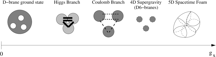
Figure 3: The different phases as we increase $g_{s}$.

To prove our proposals there are several further steps that must be taken

1. We must demonstrate that there are enough microstates constructed from 1/2-BPS “atoms” to account for the known entropy of the black hole carrying the total charge of the system.

2. We should show that the typical microstate at finite string coupling has a complex structure out to the horizon scale, but that the detailed microstructure is inaccessible to a conventional semiclassical observer.

3. We must complete our understanding of the relation of the Coulomb and Higgs branches of quiver gauge theories, in particular whether spacetime constraints such as triangle inequalities are realized in the Higgs branch also.

4. We must understand the role of the superpotentials that appear in quivers with closed loops in determining the structure of the Higgs branch moduli space, and whether and how this affects the flow of states between these branches as the coupling changes.

While these are challenging problems, solving them is important for understanding the quantum mechanical states underlying classical spacetimes.

Acknowledgments:

We thank Jan de Boer, Frederick Denef, Michael Douglas, Sergio Ferrara, Davide Gaiotto, Ori Ganor, Renata Kallosh, Boris Pioline and Joan Simón for useful discussions. This work was supported by the DOE grant DE-FG02-95ER40893 (VB,TL), the NSF grant PHY-0331728 (VB,TL), and a dissertation fellowship from the University of Pennsylvania (TL). The work of EG was supported by the US Department of Energy under contracts DE-AC03-76SF00098 and DE-FG03-91ER-40676 and by the National Science Foundation under grant PHY-00-98840. VB thanks the Weizmann Institute for hospitality while this paper was completed. EG and VB would like to dedicate this paper to the memory of John Brodie and Andrew Chamblin.

Appendix A The central charge for $\alpha=0$

The calculation of the ${\cal N}=2$ central charge is outlined in [61] and is given by

$$Z_{p}=F_{\mu}p_{p}^{\mu}-X^{\mu}q^{p}_{\mu},$$ (A.1)

where $X^{\mu}$ are the projective coordinates for the four-dimensional scalars

$$X^{0} = {-1\over\sqrt{J_{4}}}{\partial J_{4}\over\partial K^{0}}-iM_{0}\to i\ \ \rm{as}\ \rho\to\infty,$$

$$X^{i} = {-1\over\sqrt{J_{4}}}{\partial J_{4}\over\partial M_{j}}+iK^{j}\to(-1+i\delta K^{j}).$$ (A.2)

$F_{\mu}=\partial F(X)/\partial X^{\mu}$ is the derivative of the cubic prepotential

$$F(X)=-{X^{1}X^{2}X^{2}\over X^{0}}.$$ (A.3)

In the conventions of [61] the magnetic and electric charges for the $p$th brane are given by

$$p^{0} = {L\over 2}n_{p},\ \ \ \ \ p^{j}={1\over 2}d^{j}_{p}$$

$$q_{0} = {1\over 2L^{2}}{d^{1}_{p}d^{2}_{p}d^{3}_{p}\over n_{p}^{2}},\ \ \ q_{i}=-{1\over 2L}s_{ijk}{d^{j}_{p}d^{k}_{p}\over 2n_{p}}.$$ (A.4)

Putting this all together we find

$$Z_{p}={L\over 2}n_{p}-{1\over 2L}\sum_{i,j,k}{s_{ijk}\over 2}n_{p}\lambda^{j}_{p}\lambda^{k}_{p}+{i\over 2}\Psi_{p}\,.$$ (A.5)

The mass of the $p$th brane is given by

$$m_{p}={|Z_{p}|\over 4G_{4}}.$$ (A.6)

Note that the total central charge is $Z=\sum_{p}Z_{p}$, and that

$$Im[Z]={1\over 2}\sum_{p}\Psi_{p}=0$$ (A.7)

because of the integrability constraint and the fact that we have set $\alpha$ in (3.3) to zero for simplicity.

Appendix B Non-zero $\alpha$

In general, for non-zero values of $\alpha$ the situation is more complicated as the reduction from five to four dimensions is now along a fiber of a slightly different magnitude (a similar situation arises in [23]).

Let us consider how $\alpha\neq 0$ affects the phase of the central charge $Z$ as defined above. Note first that the expression $Im[Z_{p}]={1\over 2}\Psi_{p}=2\!<\!\!\Gamma_{p},\Gamma_{\infty}\!\!>$ is a trivial consequence of equations (A.1), (A) and the explicit form for the $F_{\mu}$’s:

$$F_{0}={+1\over\sqrt{J_{4}}}{\partial J_{4}\over\partial M_{0}}+iK_{0},\qquad F_{i}={-1\over\sqrt{J_{4}}}{\partial J_{4}\over\partial K^{j}}+iK_{j}.$$ (B.1)

This implies that eq. (A.7) still holds, hence the central charge is real and $\alpha$ cannot be it’s phase! It turns out that the phase $\alpha$ of the central charge used in [27, 29, 13] is defined in a different gauge, where a Kahler transformation has been used to fix the asymptotic value of $X^{0}\to i$. As we will demonstrate, for non-zero $\alpha$ our asymptotic value for $X_{0}$ is $ie^{-i\alpha}$. Rotating this back to the Denef etal.’s gauge implies that the central charge picks up an overall phase of $\alpha$. Hence $\alpha$ is the phase of of the central charge in Denef etal.’s gauge. Note that the expression $\Psi_{p}=4\!<\!\!\Gamma_{p},\Gamma_{\infty}\!\!>$ is gauge invariant. We will demonstrate that even for non-zero $\alpha$ the FI terms $\theta_{p}$ are stil exactly equal to $(8G_{4})^{-1}\Psi_{p}$, as expected.

B.1 Redefining the harmonics for $\alpha\neq 0$

We start by observing that for non-zero $\alpha$ as defined in eq. (3.3) the asymptotic value of $k_{0}$ becomes ${L\over 2}\sin\alpha$. This implies that if we left our definitions for the harmonic functions $M^{\mu},K_{\mu}$ unchanged, the asymptotic value for $J_{4}$ would now be $\cos^{2}\alpha<1$. To remedy this situation we need to adjust the reduction of our five-dimensional solution to four dimensions as follows. First we recognize that the IIA coupling constant is now $g_{s}l_{s}=L\cos\alpha=R$, but we still define the new radial coordinate $\rho=2r/L$. The time coordinate now also needs to be rescaled $t^{(4D)}=\sec\alpha\,t^{(5D)}$. The new harmonic functions are:

$$M_{0}=-\cos\alpha\,HL^{2}/4,\;\;K^{0}=\sec^{2}\alpha\,4K/L,\;\;K^{i}=Lh^{i},\;\;M_{i}=\sec\alpha\,M_{i}^{5D},$$ (B.2)

with similar scalings for $\Gamma$. With these definitions, $J_{4}(x)=I_{4}({\cal H}(x))\to 1$ at $\infty$. The asymptotic value for $X^{0}$ is now $X^{0}\to\sin\alpha+i\cos\alpha=ie^{-i\alpha}$ as previously advertised.

B.2 Checking the FI term

In the gauge of Denef etal., it also possible to write down the individual contribution to the central charge from each center as:

$$Z_{p}={R\over 2}n_{p}\prod_{i}(1+iB^{i}_{p})=4G_{4}\,m_{p}\,e^{i\alpha_{p}},$$ (B.3)

where the $B^{i}_{p}=\left({d_{p}^{i}\over Rn_{p}}-{\delta K^{i}\over\cos\alpha}+{\sin\alpha\over\cos\alpha}\right)$ are the normalized (F-B) terms on each $D6$-brane. This allows to quickly check that we have the right definition for the $FI$ term:

$$(8G_{4})\,\theta_{p} = 2|Z_{p}|\sin(\alpha_{p}-\alpha)$$

$$= 2|Z_{p}|\sin\alpha_{p}\cos\alpha-2|Z_{p}|\cos\alpha_{p}\sin\alpha$$

$$= Rn_{p}\,Re\left[\prod_{i}(1+iB^{i}_{p})\right]\cos\alpha-Rn_{p}\,Im\left[\prod_{i}(1+iB^{i}_{p})\right]\sin\alpha$$

$$= Rn_{p}\left[\sum_{i}B^{i}_{p}-\prod_{i}B^{i}_{p}\right]\cos\alpha-Rn_{p}\left[1+\sum_{i}{s_{ijk}\over 2}\,B^{j}_{p}B^{k}_{p}\right]\sin\alpha$$

$$= {n_{p}\over\cos\alpha}\left(\sum_{i}\lambda^{i}_{p}-{1\over L^{2}}\prod_{i}\lambda^{i}_{p}+2L\sin\alpha\right)$$

$$= \Psi_{p}^{4D}=4<\Gamma_{p},\Gamma_{\infty}>=\Psi_{p}^{5D}/\cos\alpha.$$ (B.5)

Here we have differentiated $\Psi_{p}^{4D}=4<\Gamma_{p},\Gamma_{\infty}>$ which is defined canonically in $D=4$ from the renormalized charge vectors $\Gamma_{p}$ from 5D inspired $\Psi_{p}^{5D}$ defined by simply adding a correction term $(2Ln_{p}\sin\alpha)$ to the right-hand side of eq.(3.6).

References

- [1] A. Sen, “Extremal black holes and elementary string states,” Mod. Phys. Lett. A10 (1995) 2081–2094, hep-th/9504147.
- [2] A. Strominger and C. Vafa, “Microscopic Origin of the Bekenstein-Hawking Entropy,” Phys. Lett. B379 (1996) 99–104, hep-th/9601029.
- [3] S. D. Mathur, “The fuzzball proposal for black holes: An elementary review,” Fortsch. Phys. 53 (2005) 793–827, hep-th/0502050.
- [4] S. D. Mathur, “The quantum structure of black holes,” hep-th/0510180.
- [5] I. Bena and N. P. Warner, “Bubbling supertubes and foaming black holes,” hep-th/0505166.
- [6] P. Berglund, E. G. Gimon, and T. S. Levi, “Supergravity microstates for BPS black holes and black rings,” hep-th/0505167.
- [7] I. Bena, C.-W. Wang, and N. P. Warner, “The foaming three-charge black hole,” hep-th/0604110.
- [8] V. Balasubramanian, P. Kraus, and M. Shigemori, “Massless black holes and black rings as effective geometries of the D1-D5 system,” Class. Quant. Grav. 22 (2005) 4803–4838, hep-th/0508110.
- [9] H. Lin, O. Lunin, and J. Maldacena, “Bubbling AdS space and 1/2 BPS geometries,” JHEP 10 (2004) 025, hep-th/0409174.
- [10] V. Balasubramanian, J. de Boer, V. Jejjala, and J. Simon, “The library of Babel: On the origin of gravitational thermodynamics,” JHEP 12 (2005) 006, hep-th/0508023.
- [11] V. Balasubramanian, B. Czech, K. Larjo, and J. Simon, “Integrability vs. information loss: A simple example,” hep-th/0602263.
- [12] V. Balasubramanian, D. Marolf, and M. Rozali, “Information recovery from black holes,” hep-th/0604045.
- [13] F. Denef, “Quantum quivers and Hall/hole halos,” JHEP 10 (2002) 023, hep-th/0206072.
- [14] R. Dijkgraaf, C. Vafa, and E. Verlinde, “M-theory and a topological string duality,” hep-th/0602087.
- [15] I. Bena and N. P. Warner, “One ring to rule them all … and in the darkness bind them?,” hep-th/0408106.
- [16] J. P. Gauntlett, J. B. Gutowski, C. M. Hull, S. Pakis, and H. S. Reall, “All supersymmetric solutions of minimal supergravity in five dimensions,” Class. Quant. Grav. 20 (2003) 4587–4634, hep-th/0209114.
- [17] H. S. Reall, “Higher dimensional black holes and supersymmetry,” Phys. Rev. D68 (2003) 024024, hep-th/0211290.
- [18] R. Kallosh and B. Kol, “E(7) Symmetric Area of the Black Hole Horizon,” Phys. Rev. D53 (1996) 5344–5348, hep-th/9602014.
- [19] V. Balasubramanian, “How to count the states of extremal black holes in N = 8 supergravity,” hep-th/9712215.
- [20] M. Cvetic and A. A. Tseytlin, “Solitonic strings and BPS saturated dyonic black holes,” Phys. Rev. D53 (1996) 5619–5633, hep-th/9512031.
- [21] S. Ferrara and J. M. Maldacena, “Branes, central charges and -duality invariant BPS conditions,” Class. Quant. Grav. 15 (1998) 749–758, hep-th/9706097.
- [22] D. Gaiotto, A. Strominger, and X. Yin, “New connections between 4D and 5D black holes,” JHEP 02 (2006) 024, hep-th/0503217.
- [23] H. Elvang, R. Emparan, D. Mateos, and H. S. Reall, “Supersymmetric 4D rotating black holes from 5D black rings,” hep-th/0504125.
- [24] I. Bena, P. Kraus, and N. P. Warner, “Black rings in Taub-NUT,” hep-th/0504142.
- [25] D. Marolf, “Chern-Simons terms and the three notions of charge,” hep-th/0006117.
- [26] E. Cremmer and B. Julia, “The SO(8) supergravity,” Nucl. Phys. B159 (1979) 141.
- [27] F. Denef, “Supergravity flows and D-brane stability,” JHEP 08 (2000) 050, hep-th/0005049.
- [28] F. Denef, B. R. Greene, and M. Raugas, “Split attractor flows and the spectrum of BPS D-branes on the quintic,” JHEP 05 (2001) 012, hep-th/0101135.
- [29] B. Bates and F. Denef, “Exact solutions for supersymmetric stationary black hole composites,” hep-th/0304094.
- [30] K. Behrndt, R. Kallosh, J. Rahmfeld, M. Shmakova, and W. K. Wong, “STU black holes and string triality,” Phys. Rev. D54 (1996) 6293–6301, hep-th/9608059.
- [31] L. Andrianopoli, R. D’Auria, S. Ferrara, P. Fre, and M. Trigiante, “E(7)(7) duality, BPS black-hole evolution and fixed scalars,” Nucl. Phys. B509 (1998) 463–518, hep-th/9707087.
- [32] S. Ferrara and R. Kallosh, “On N = 8 attractors,” hep-th/0603247.
- [33] S. Ferrara, E. G. Gimon, and R. Kallosh, “Magic Supergravities, N=8 and Black Hole Composites,” to appear...
- [34] I. Bena and P. Kraus, “Microscopic description of black rings in AdS/CFT,” JHEP 12 (2004) 070, hep-th/0408186.
- [35] M. J. Duff, J. T. Liu and J. Rahmfeld, Nucl. Phys. B 459, 125 (1996) [arXiv:hep-th/9508094].
- [36] M. J. Duff and J. Rahmfeld, Phys. Lett. B 345, 441 (1995) [arXiv:hep-th/9406105].
- [37] M. J. Duff and J. Rahmfeld, Nucl. Phys. B 481, 332 (1996) [arXiv:hep-th/9605085].
- [38] J. Rahmfeld, Phys. Lett. B 372, 198 (1996) [arXiv:hep-th/9512089].
- [39] J. M. Maldacena and A. Strominger, “Statistical Entropy of Four-Dimensional Extremal Black Holes,” Phys. Rev. Lett. 77 (1996) 428–429, hep-th/9603060.
- [40] C. V. Johnson, R. R. Khuri, and R. C. Myers, “Entropy of 4D Extremal Black Holes,” Phys. Lett. B378 (1996) 78–86, hep-th/9603061.
- [41] V. Balasubramanian and F. Larsen, “On D-Branes and Black Holes in Four Dimensions,” Nucl. Phys. B478 (1996) 199–208, hep-th/9604189.
- [42] I. R. Klebanov and A. A. Tseytlin, “Intersecting M-branes as four-dimensional black holes,” Nucl. Phys. B475 (1996) 179–192, hep-th/9604166.
- [43] J. M. Maldacena, A. Strominger, and E. Witten, “Black hole entropy in M-theory,” JHEP 12 (1997) 002, hep-th/9711053.
- [44] O. Lunin and S. D. Mathur, “AdS/CFT duality and the black hole information paradox,” Nucl. Phys. B623 (2002) 342–394, hep-th/0109154.
- [45] O. Lunin and S. D. Mathur, “Statistical interpretation of Bekenstein entropy for systems with a stretched horizon,” Phys. Rev. Lett. 88 (2002) 211303, hep-th/0202072.
- [46] S. D. Mathur, “A proposal to resolve the black hole information paradox,” Int. J. Mod. Phys. D11 (2002) 1537–1540, hep-th/0205192.
- [47] M. R. Douglas and G. W. Moore, “D-branes, Quivers, and ALE Instantons,” hep-th/9603167.
- [48] M. Berkooz, M. R. Douglas, and R. G. Leigh, “Branes intersecting at angles,” Nucl. Phys. B480 (1996) 265–278, hep-th/9606139.
- [49] V. Balasubramanian and R. G. Leigh, “D-branes, moduli and supersymmetry,” Phys. Rev. D55 (1997) 6415–6422, hep-th/9611165.
- [50] M. Berkooz and H. L. Verlinde, “Matrix theory, AdS/CFT and Higgs-Coulomb equivalence,” JHEP 11 (1999) 037, hep-th/9907100.
- [51] E. Witten, “Phases of N = 2 theories in two dimensions,” Nucl. Phys. B403 (1993) 159–222, hep-th/9301042.
- [52] E. Witten, “On the conformal field theory of the Higgs branch,” JHEP 07 (1997) 003, hep-th/9707093.
- [53] M. Reineke, “The Harder-Narasimhan system in quantum groups and cohomology of quiver moduli,” math.QA/0204059.
- [54] D. Gaiotto, A. Simons, A. Strominger, and X. Yin, “D0-branes in black hole attractors,” hep-th/0412179.
- [55] D. Gaiotto, M. Guica, L. Huang, A. Simons, A. Strominger, and X. Yin, “D4-D0 branes on the quintic,” JHEP 03 (2006) 019, hep-th/0509168.
- [56] D. Gaiotto, A. Strominger, and X. Yin, “From AdS(3)/CFT(2) to black holes / topological strings,” hep-th/0602046.
- [57] E. Witten, “BPS bound states of D0-D6 and D0-D8 systems in a B-field,” JHEP 04 (2002) 012, hep-th/0012054.
- [58] M. R. Douglas, D. Kabat, P. Pouliot, and S. H. Shenker, “D-branes and short distances in string theory,” Nucl. Phys. B485 (1997) 85–127, hep-th/9608024.
- [59] T. Banks, W. Fischler, S. H. Shenker, and L. Susskind, “M theory as a matrix model: A conjecture,” Phys. Rev. D55 (1997) 5112–5128, hep-th/9610043.
- [60] D. Cremades, L. E. Ibanez, and F. Marchesano, “Yukawa couplings in intersecting D-brane models,” JHEP 07 (2003) 038, hep-th/0302105.
- [61] M. Billo et al., “The 0-brane action in a general D = 4 supergravity background,” Class. Quant. Grav. 16 (1999) 2335–2358, hep-th/9902100.