Eternal inflation: The inside story

Abstract

Motivated by the lessons of black hole complementarity, we develop a causal patch description of eternal inflation. We argue that an observer cannot ascribe a semiclassical geometry to regions outside his horizon, because the large-scale metric is governed by the fluctuations of quantum fields. In order to identify what is within the horizon, it is necessary to understand the late time asymptotics. Any given worldline will eventually exit from eternal inflation into a terminal vacuum. If the cosmological constant is negative, the universe crunches. If it is zero, then we find that the observer’s fate depends on the mechanism of eternal inflation. Worldlines emerging from an eternal inflation phase driven by thermal fluctuations end in a singularity. By contrast, if eternal inflation ends by bubble nucleation, the observer can emerge into an asymptotic, locally flat region. As evidence that bubble collisions preserve this property, we present an exact solution describing the collision of two bubbles.

I Introduction

Theories with multiple metastable vacua tend to exhibit the cosmological dynamics known as eternal inflation ColDel80 ; GutWei83 ; Vil83b ; Lin86b . This is usually described in terms of a spacetime far larger than the presently visible region. Every vacuum is realized, over and over, in different regions of this ever-expanding universe. A longstanding problem has been to compute the probability that a given vacuum will be observed.

Empirically, the small nonzero value of the cosmological constant Rie98 suggests that the number of metastable vacua is extremely large Sak84 ; Wei87 . On the theoretical side, string theory appears to satisfy this requirement BP ; KKLT . Eternal inflation populates the landscape. Hence, the notorious problem of a probability measure has received renewed interest.

There are actually two kinds of eternal inflation. False vacuum eternal inflation (FVEI) is driven by the de Sitter expansion of the metastable vacua themselves. They decay when bubbles of lower energy vacua form spontaneously. But inflation perdures because the bubbles do not grow fast enough to catch up with the de Sitter expansion of the false vacuum inside of which they formed GutWei83 . Thus eventually all allowed transitions, no matter how suppressed, will take place in different regions of the universe, and the landscape is populated. The global picture is that of an infinite universe containing infinitely many bubbles, nested inside each other or expanding in different places, occasionally colliding but never percolating (Fig. 1). In some bubbles inflation can end locally. If the cosmological constant is negative, it ends in a big crunch; if it vanishes, then an open FRW universe is produced. If it is positive, it is still in a de Sitter phase, and further bubbles will eventually be produced.

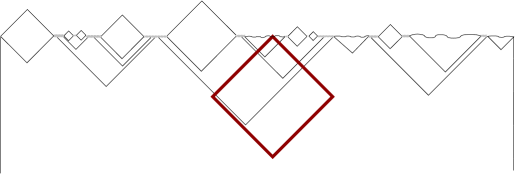
Figure 1: A conformal diagram for the global geometry in FVEI. The hats represent the future infinity of open FRW universes with vanishing cosmological constant. Regions with negative cosmological constant end in a big crunch singularity (squiggly lines). The part of the universe which remains in the inflationary phase has zero comoving volume but infinite physical volume. The thick diamond shows an example of a causally connected region accessible to a single observer. The local description developed here is confined to such regions.

Slow-roll eternal inflation (SREI) does not rely on local minima in the potential. Instead, it requires a potential $V$ in which a scalar field $\phi$ classically rolls down slowly. If $dV/d\phi\ll V^{3/2}$, the quantum fluctuations of the scalar field dominate over its classical evolution, and the field undergoes a kind of random walk Linde ; GonLin87 . In some regions of the inflating universe, the field will wander into a regime where the classical evolution dominates and inflation can end. But there will always be other regions in which the field fluctuates up and the inflationary expansion continues. If more than one final vacuum is accessible from the SREI regime, or if certain moduli can be driven to different values during SREI, one would again like to compute the probabilities for different outcomes.

Intuitively, one might expect the probability to be proportional to the fraction of the volume of the universe taken up by the vacuum in question. But this prescription is ill-defined. In eternal inflation there is no preferred foliation of spacetime into spatial slices, and different choices lead to radically different answers LinLin96 . This is easily seen as follows. In a region occupied by one vacuum, there can be preferred slices, for example the comoving slices that are orthogonal to the four-velocity of the cosmic fluid. In our region, those are the slices on which the universe appears homogeneous and isotropic. During ordinary slow-roll inflation, de Sitter invariance is broken by the time-dependence of the inflaton field, and the hypersurfaces of constant inflaton field provide a preferred slicing.

But there is no natural, unique way of extending such slices to cover different vacua separated by an inflating region. The problem is that by assumption, any global slice through the geometry must include regions that are in the eternally inflating phase. In regions trapped in a false vacuum, the geometry is locally de Sitter invariant. The case of slow-roll eternal inflation is similar. When quantum fluctuations dominate over the classical slow-roll, hypersurfaces of constant density will not be spacelike, restoring for all practical purposes the local de Sitter invariance.

But there are reasons to believe that a global description must be inconsistent SusTho93 . In the context of black holes, it leads to sharp paradoxes that are resolved only if we describe one observer at a time. This suggests more generally that we cannot talk simultaneously about two observers who are forever out of causal contact. (Since they can never compare their experiences, this is not a restriction on our ability to describe the world.) Perhaps, then, the ambiguities and paradoxes of eternal inflation are due, at least in part, to our insistence on a global point of view.

The goal of this paper is to begin exploring a local description. What does eternal inflation look like to a single observer?

We begin, in Sec. II, by asking whether a single observer can predict the geometry of regions behind his event horizon. This is not obviously impossible. For example, we can predict with some confidence the interior geometry of a black hole formed from stellar collapse, even if we remain forever outside. However, this ability depends on the assumption that the gravitational backreaction of quantum fluctuations is small.

To illustrate this point, we consider a thought experiment. An apparatus measures the spin of an electron after both electron and apparatus fall into a black hole. Thanks to standard decoherence effects, the apparatus will show a definite outcome after the measurement. But the outside observer is ignorant of the outcome, and thus cannot predict which of two macroscopically distinguishable events will take place inside the black hole. But if the pointer of the apparatus is very massive, the metric inside the black hole will depend on its position. Hence, the outside observer cannot predict a definite metric for the black hole interior.

This argument generalizes to any situation in which part of the spacetime remains inaccessible to a given observer and the metric depends strongly on the outcome of quantum fluctuations. By definition, both of these conditions are satisfied in eternal inflation. For example, an observer cannot predict when and where bubbles of new vacua will form. He would need to describe the inaccessible regions in terms of a superposition of all possible decay sequences. Because the formation of a bubble affects the large-scale geometry, this task transcends the realm of semiclassical gravity. Therefore, a local observer in eternal inflation cannot consistently define a global geometry.

We conclude that the local and the global point of view are really inequivalent. This is encouraging since it opens the possibility for a probability measure to arise naturally from the local point of view, without the ambiguities that plague the global description Bou06 . (If eternal inflation admits no global, classical geometry, then the problem is not which slicing to pick. The problem is that there is nothing to slice.)

The remainder of the paper is devoted to an analyzing how local observers experience an eternally inflating universe. An important difference to the global view is that for any one observer, inflation will eventually end (except if all vacua have positive energy—a relatively simple case that is hard to reconcile with observation DysKle02 ). We focus not only on observations during eternal inflation, but also consider the observer’s fate in the asymptotic future after inflation has ended. We distinguish between SREI (slow roll eternal inflation) and FVEI (false vacuum eternal inflation).

In Sec. III, we review the conventional global description of SREI. We then offer a local description. A typical worldline in SREI experiences nothing more than ordinary slow-roll. In particular, the entropy will not decrease by more than 1 as a result of fluctuations, as required by the second law of thermodynamics.

Along any given geodesic, SREI eventually must end. If the effective cosmological constant becomes negative, there will be a big crunch, long before the scales that left the horizon during SREI would re-enter. In regions with positive cosmological constant, the same censorship is achieved by a de Sitter horizon.

The case of zero cosmological constant is more subtle, and we treat it in more detail. Curvature perturbations become of order one precisely when scales originating in the era of SREI re-enter. Such large perturbations rapidly cause gravitational collapse, trapping the observer inside a black hole. Thus, typical observers cannot probe the scales produced during SREI.

In Sec. IV, we describe false vacuum eternal inflation (FVEI), in which the inflaton is stuck in a metastable minimum and must tunnel to exit inflation. FVEI shares many qualitative features with SREI. If several metastable vacua are available, then a typical worldline tunnels repeatedly, lowering the vacuum energy until it reaches a terminal vacuum. As in the slow-roll case, some highly atypical worldlines take a detour up to higher vacuum energy on the way to reaching a terminal vacuum.

The asymptotic structure of regions of vanishing vacuum energy differs strongly from SREI. In the leading approximation, FVEI produces an open FRW universe in which perturbations stop growing after curvature dominates. A more careful treatment should take into account collisions with other bubbles of true vacuum GutWei83 . We construct an exact solution describing the collision of two zero cosmological constant bubbles in an ambient de Sitter space. We assume that the energy of the colliding walls is converted to dust. Even in this worst case scenario, we find that bubble collisions do not cause gravitational collapse. Hence, the asymptotic conformal structure is that of an unperturbed open FRW universe (the hats shown in Fig. 1). Asymptotic observers do not fall into black holes, and can look back on the infinite cluster of bubbles colliding with their own.

The appendix summarizes various results on slow roll inflation used in the main text.

II Predicting the geometry behind the horizon

The macroscopic geometry inside a black hole can usually be predicted by an external observer, if initial conditions are known. In this section we show that this becomes impossible if the geometry depends strongly on the outcome of quantum measurements in the invisible region. This implies that semiclassical gravity cannot describe the region behind the horizon of a local observer in eternal inflation.

II.1 A gedankenexperiment involving a black hole

Consider the gedankenexperiment shown in Fig. 2. An electron is prepared in a linear superposition of spin-up and spin-down, $|\psi\rangle=\alpha\,|\!\!\!\uparrow\rangle+\beta\,|\!\!\!\downarrow\rangle$, and placed inside an apparatus. Then the entire apparatus, including the electron, is thrown into a very large black hole. The apparatus is programmed to measure the spin only after crossing the event horizon of the black hole, but well before it reaches regions whose curvature is important on the scale of the apparatus.

Because the apparatus is freely falling, and because curvature is negligible, the measurement of the spin proceeds exactly as it would in flat space. The apparatus couples to the spin, resulting in the joint state

$$|\Psi\rangle=\alpha\,|\!\uparrow\rangle_{A}\otimes\,|\!\uparrow\rangle+\beta\,|\!\downarrow\rangle_{A}\otimes\,|\!\downarrow\rangle~{}.$$ (1)

The subscript $A$ refers to the state vector in the Hilbert space of the apparatus. Of course, a superposition of macroscopically different states, such as the apparatus pointing up and pointing down, is never observed, and we understand why. A macroscopic object cannot be insulated from the environment; for example, it will emit infrared photons.

Thus, a full description must include the environment. What is perceived as the apparatus will really be entangled with many external degrees of freedom that cannot be observed and thus are implicitly traced over. One can show Schl03 that this results in a density matrix describing the apparatus-electron part of the world, with probability $|\alpha|^{2}$ for the state $|\!\uparrow\rangle_{A}\otimes\,|\!\uparrow\rangle$ and probability $|\beta|^{2}$ for the state $|\!\downarrow\rangle_{A}\otimes\,|\!\downarrow\rangle$. The description of the apparatus alone thus exhibits decoherence, which allows us to understand the apparent nonunitarity of a definite measurement outcome in terms of a lack of information about inaccessible degrees of freedom.

However, the description from the point of view of an observer outside the black hole is very different. From her point of view, the information contained in the infalling apparatus is imprinted on the black hole horizon. After the black hole evaporates, the information will be encoded in Hawking radiation. (At least, the weight of the evidence from string theory suggests that this is a unitary process.) Thus, while the outside observer can predict that the apparatus will measure the electron, she cannot ever state that the electron was measured to be up (or down). Because the apparatus becomes correlated with the electron, she would ascribe to the black hole interior a superposition of macroscopically distinguishable states.

This can be understood also as follows. From the outside point of view, the black hole includes all the degrees of freedom that the apparatus can interact with after measuring the electron. That is, it includes the whole environment accessible to the apparatus. With these degrees of freedom included, the evolution should indeed be unitary. Thus, a natural extrapolation of the outside data implies that the electron, apparatus, and the rest of the black hole interior remain in a superposition of “up” and “down”.

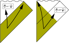
Figure 2: On the left, a spin is measured after the apparatus has entered a black hole, leaving the outside observer ignorant of the outcome. On the right, the measurement takes place outside the black hole, beyond the causal past of an infalling observer. Either way, the observer cannot ascribe a definite outcome to the measurement. If the geometry depends on this outcome, it cannot be treated semiclassically, since it would involve a quantum superposition of macroscopically distinct metrics.

Now suppose that the apparatus involves very massive moving parts. For example, its pointer may be a neutron star, which is moved to different places depending on whether the electron spin is up or down. The point is to arrange for the gravitational field inside the black hole to depend strongly, and macroscopically, on the outcome of the measurement. We concluded earlier that from the outside point of view, the black hole interior must be described by a superposition of macroscopically distinguishable states. Now we see that this may involve a superposition of very different metrics. Therefore, there is no unique semiclassical geometry that can be predicted for the black hole interior by an exterior observer, even if the initial quantum state is known exactly.

Normally, two different observers would agree on the outcome of a quantum-mechanical measurement. What distinguishes the above gedankenexperiment is that the location of the experiment, the black hole interior, never enters the past of the outside observer. Therefore the outside observer (and more importantly, environmental degrees of freedom she interacts with) never get to look at the apparatus after the measurement. It is not particularly important that the causal separation happens to manifest itself in a black hole event horizon.

In fact, we can easily switch roles. Suppose now that the apparatus containing the electron remains far outside the black hole, and is programmed to measure the spin of the electron at a time $t_{0}$. Consider an observer who falls into the black hole and ends up at the singularity, as shown in Fig. 2. This observer’s causal past does not include all of the black hole exterior. If $t_{0}$ is chosen sufficiently late, then the infalling observer cannot witness the decoherence of the apparatus, and so he cannot predict a unique semiclassical geometry for the outside region.

This illustrates that the relevant causal boundary is simply the boundary of the past of the observer’s worldline. In the first experiment, this happens to be a horizon. In the second, it is the past light-cone of the observer at the moment when he hits the singularity. The only difference is that in the second case, there are additional uncertainties because of unknown initial conditions at a portion of past null infinity. We will not be interested here in this trivial obstacle to predictability; where necessary, we will assume that initial conditions are completely known.

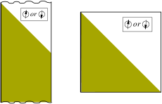
Figure 3: Examples of causal horizons in cosmology: A closed FRW universe (left) and de Sitter space (right). The observer is on the left edge of each diagram. She cannot access the result of the measurement in the (white) region outside her causal past.

Therefore, our reasoning generalizes to other nontrivial spacetimes, and in particular, to cosmology. Examples are shown in Fig. 3: an observer hitting a big crunch, and an observer surrounded by a cosmological horizon in de Sitter space.

Let us summarize. The emergence of classical behavior, including classical geometry, depends on the separation of degrees of freedom into gross, observed features and unobserved “environmental” degrees of freedom. The selection of a definite outcome from the possibilities allowed by the resulting density matrix cannot be unitarily predicted from initial data. But the metric generally depends on this outcome. Therefore, an observer cannot ascribe a unique geometry to regions that are forever outside his past, even if initial conditions are known and even if another observer, entering such a region, can be sure to find a well-defined geometry.

II.2 Eternal inflation

Now let us apply this result to eternal inflation. In FVEI, an infinite number of bubbles are nucleated globally, but most will be outside the observer’s horizon. Hence, to the observer, they cannot be ascribed a definite place and time. From a field theory point of view, the region beyond the horizon would need to be described by a wave function with slowly increasing support in the lower energy vacua. When gravity is included, this corresponds to a superposition of different geometries.

SREI relies on the thermal fluctuations of the inflaton field. We assume that inflation eventually ends for any observer, so most of the SREI regime is outside the observer’s horizon. The fluctuations in this region do not decohere. (In fact, the results of the following two sections show that that they are unlikely to decohere even inside the horizon.) In particular, it is impossible to identify specific spacetime regions where the unlikely repeated upward fluctuations occur that drive SREI. From a field theory point of view, the wavefunction for the inflaton field simply spreads out outside the horizon. In most places the spread is not large enough to dominate over the classical evolution, and an approximate geometry can be assigned. But SREI is eternal only due to the tails of this wavefunction. In the usual description, these tails set the classical value of the field in a small fraction of the spacetime volume. The single observer cannot know where, and thus cannot assign a definite geometry.

Note that we did not assume an ignorance of initial conditions. If one imagines that the universe was created, perhaps by “tunneling from nothing”, there might be an initial hypersurface, and generically, an observer’s past lightcone will only include a fraction of that surface. However, for the purposes of our argument we can happily assume that the observer knows the entire initial data, perhaps because they are fixed by some physical law (e.g., the no-boundary proposal).

The point is that a definite geometry is incompatible with the unitary quantum evolution of any initial data that lead to eternal inflation. A semiclassical description of the geometry depends on the decoherence of quantum effects such as bubble formation and field fluctuations. The geometry in our past is classical precisely because of nonunitarity: it has decohered to one shape and not another. But from a local observer’s point of view, the regions beyond the horizon remain in quantum superposition.

III Slow-roll eternal inflation

We will begin this section with a summary of the conventional global description of slow-roll eternal inflation (SREI) Lin86b ; GonLin87 . We will then describe the experience of a typical local observer, who simply experiences conventional slow-roll inflation. He will end up in the vacuum that lies along the gradient from his starting point. We shall see that this behavior is in fact required by the second law of thermodynamics. We will show that at late times, all geodesics end on a singularity.

The enormous differences between the global and local description should not come as a surprise. SREI relies on unusually large or persistent upward fluctuations of the inflaton field. The global picture compensates for the extreme rarity of such events by rewarding them with large volume expansion factors. But from the local point of view, such fluctuations are simply extremely unlikely, with no compensating features. For the reasons given in Sec. II, volume factors in unobservable regions are meaningless.

III.1 Conventional global description

The conventional argument for slow-roll eternal inflation goes as follows. Consider one Hubble volume during slow-roll inflation. After one Hubble time, it will have expanded to $e^{3}\approx 20$ new Hubble volumes. Meanwhile, the expectation value of the inflaton field will have decreased by an amount

$$\Delta\phi=\frac{|\dot{\phi}|}{H}=\frac{V^{\prime}}{3H^{2}}=\frac{H^{\prime}}{4\pi H}$$ (2)

from rolling classically down the potential $V(\phi)$.

By Eq. (79), the quantum fluctuations of $\phi$ on the Hubble scale are given by

$${\cal P}_{\phi}^{1/2}(H)=\frac{H}{2\pi}~{}.$$ (3)

A measurement of the inflaton field should yield values in a Gaussian distribution about the classical value of $\phi$, with standard deviation $H/2\pi$. The Hubble scale quantum fluctuations will dominate over the classical evolution if

$$\frac{H^{2}}{H^{\prime}}\gtrsim 1~{}.$$ (4)

Let us suppose that this condition is comfortably satisfied: $H^{2}/H^{\prime}\gg 1$. Then every Hubble time, approximately half of the 20 new Hubble volumes should witness an increase in the inflaton field value. Instead of rolling down, these ten Hubble volumes will have climbed up the inflationary potential.

Of course, the other ten Hubble volumes will see a decrease of $\phi$, mostly due to downward quantum fluctuations rather than classical slow-roll. Over time, some regions evolve into a regime where $H^{2}/H^{\prime}<1$. Thus, regions are produced where classical evolution dominates, and inflation can come to an end.

To get eternal inflation, it is enough that $\phi$ increases in at least one new Hubble volume every Hubble time. For this, it suffices to demand $H^{2}/H^{\prime}\gtrsim 1$. Then there will always be some regions where inflation continues. Inflation is globally eternal and ends only locally.

Let us assume that the inflaton potential vanishes at the global minimum $\phi=0$ and contains a quantum-dominated regime:

$$H^{2}/H^{\prime}>1~{}~{}~{}~{}\mbox{for all}~{}\phi>\phi_{\rm qc}~{}.$$ (5)

We will refer to $\phi_{\rm qc}$, and the era when this value is attained, as the quantum/classical boundary. For definiteness, we take $\phi_{\rm qc}>0$ to be positive. We also assume that $V\ll 1$ in the quantum-dominated regime. It should be stressed that SREI does not require Planck scale densities or curvatures.

Not all sensible inflationary potentials contain such a regime. But it is fairly generic, in that it requires only that the potential contain portions that are sufficiently high (for a large effective cosmological constant to drive the quantum fluctuations) and not too steep (so that the classical slow-roll is negligible). For example, let us suppose that the inflaton potential was $V=m^{2}\phi^{2}/2$, with no corrections even for large $\phi$, and with $m\sim O(10^{-6})$. Then the quantum-dominated regime corresponds to $\phi\gtrsim m^{-1/2}$ (see Fig. 4).

Figure 4: The slow-roll potential $V=\frac{1}{2}m^{2}\phi^{2}$. The SREI regime is $\phi>m^{-1/2}$.

In this example, the inflaton would have been at the classical/quantum boundary, $\phi_{\rm qc}\sim m^{-1/2}$, at a very early time during inflation, namely $O(m^{-1})$ e-foldings before entering the range, $\phi\sim O(1)$, that created the presently visible universe. Correspondingly, we would have to wait for the universe to expand by an enormous factor (in this example, $\exp[O(m^{-1})]$) before we could see scales that left the horizon near the eternally inflating regime. The corresponding comoving wavenumber, $k_{\rm qc}$, satisfies

$$\log\frac{k_{\rm qc}}{k_{0}}\sim O(m^{-1})~{}.$$ (6)

Thus, the scale associated with the quantum/classical boundary tends to be exponentially large compared to the scale $k_{0}$ that is presently entering the horizon. However, one could tune the inflaton potential to have a smaller separation between the observable scale and the scale corresponding to the quantum/classical boundary (see Fig. 5). Our conclusions will be independent of the size of this hierarchy.

Figure 5: A potential with a plateau supporting eternal inflation and a relatively short-lived classical slow roll.

III.2 Horizon area and second law

During the inflationary era, the local description of SREI is quite similar to that of ordinary slow roll inflation: The field rolls down classically, following the gradient of the potential. Typical quantum fluctuations are eventually overcome by classical evolution.

To see this, recall that the quantum fluctuations (the spread of the wavefunction) of $\phi$ grow like

$$\delta_{\rm q}\phi(t)\approx{H\over 2\pi}\sqrt{Ht}~{},$$ (7)

where we assume $Ht>1$; see Eq. (88). Meanwhile, the classical slow roll causes $\phi$ to decrease by

$$\Delta\phi(t)\approx|\dot{\phi}|t=\frac{V^{\prime}}{3H}t=\frac{H^{\prime}}{4\pi}t~{}.$$ (8)

The above equations hold both in SREI and in ordinary slow-roll inflation.

In SREI, the classical evolution begins to dominate after a time

$$Ht_{\rm c}=\left(2\frac{H^{2}}{H^{\prime}}\right)^{2}~{}.$$ (9)

Recall that $H^{2}/H^{\prime}>1$ in SREI, so quantum fluctuations dominate for longer than one Hubble time. During this time the field changes classically by $H^{3}/(\pi H^{\prime})$.

But classical evolution eventually wins out, and one can predict with great likelihood which vacuum it will lead to. The only case in which there is significant uncertainty of the outcome is if the field starts out within $H^{3}/H^{\prime}$ of a local maximum of the potential. In this case the observer cannot tell which side she is on.

Let us identify and resolve a possible paradox. The Bekenstein-Hawking entropy of the cosmological horizon,

$$S=\frac{A}{4}=\frac{3}{8V(\phi)},$$ (10)

depends on the effective cosmological constant $\Lambda=8\pi V(\phi)/3$, and thus on $\phi$. During classical slow-roll, $\Lambda$ will decrease, and the entropy will increase.

However, during SREI the quantum fluctuations dominate, and the area is about as likely to decrease as it is to increase. It might appear, therefore, that SREI conflicts with the second law of thermodynamics. Of course, the second law will occasionally be violated in any system, but such fluctuations must be exponentially rare. In SREI, however, area-decreasing fluctuations occur about half of the time. We will now show that SREI is nevertheless consistent with the second law.

The change in horizon area, $\delta_{\rm q}A$, induced by quantum fluctuations of the inflaton field in the time $t$, can be computed from Eq. (7). Since $A\sim H^{-2}$ one has

$$\delta_{\rm q}A(t)\sim\frac{H^{\prime}}{H^{3}}\delta_{\rm q}\phi\sim\frac{H^{\prime}}{H^{2}}\sqrt{Ht}~{}.$$ (11)

Until the time

$$\sqrt{Ht}\sim\frac{H^{2}}{H^{\prime}}~{},$$ (12)

this fluctuation is less than 1, corresponding to a negligible decrease in entropy. In particular, it follows that the quantum fluctuation during one Hubble time, $\delta_{\rm q}\phi\sim H$, causes an undetectable change in horizon area and entropy, as long as the SREI condition, Eq. (4), is satisfied.

One might be concerned that the second law does become violated after the time given in Eq. (12). But all is well, for it is precisely after this time that the classical evolution overwhelms the quantum effects, by Eq. (9).

In fact one can see this more directly. The classical increase in horizon area is given by

$$\Delta A(t)\sim[\delta_{\rm q}A(t)]^{2}~{}.$$ (13)

according to Eqs. (8) and (11). It is always positive, corresponding to an increase in entropy. It dominates ($\Delta A>\delta_{\rm q}A$) as soon as either area change becomes larger than the Planck area ($\delta_{\rm q}A>1$).

III.3 The fate of a generic observer

How about the experience of late-time postinflationary observers? We will now show that generically, their past light-cones will not grow large enough to include modes that were produced during the eternal phase. As discussed in the introduction, this is obvious if the cosmological constant is nonzero, so we will focus on the $\Lambda=0$ case.

The curvature perturbation on the comoving scale $k^{-1}$ is given by Eq. (99):

$${\cal P}_{\cal R}^{1/2}(k)=\frac{H_{*}^{2}}{H_{*}^{\prime}}~{}.$$ (14)

But according to Eq. (4), the quantum-dominated regime satisfies $H^{2}/H^{\prime}>1$. Hence, the curvature perturbations produced during this regime are of order one, and perturbation theory breaks down.

What would this look like from the point of view of a post-inflationary observer? The perturbations we see today were produced towards the end of inflation, when $H^{2}/H^{\prime}$ was small (${\cal P}_{\cal R}\sim 10^{-5}$). So first we would have to wait for an exponentially long time compared to the current age of the universe. Then we would begin to see much larger scales that left the horizon earlier in inflation, when $H^{2}/H^{\prime}$ was larger.

As we approach the time when the comoving scale $k_{\rm qc}$ enters the horizon, the spatial slices will no longer look flat but will be noticably closed or open:

$$\Omega-1\sim O(1)~{},$$ (15)

where $\Omega=\rho/\rho_{\rm c}$ and $\rho_{\rm c}=3H^{2}/8\pi$ is the critical density. Whether it looks closed or open depends on the sign of the perturbations that most recently entered the horizon; this will itself fluctuate.

When the perturbations become of order unity, overdense fluctuations will close the universe and cause gravitational collapse on a distance scale comparable to the horizon. The timescale for this collapse is also comparable to the horizon scale (i.e., the age of the universe). Thus, the observer ends up in a crunch, and cannot see further than the comoving distance $k_{\rm qc}^{-1}$.

Let us make this more precise. A region decouples from the cosmological flow and the perturbation becomes nonlinear when the density contrast, $\delta\equiv\delta\rho/\rho$, becomes of order one. The dust then stops expanding and begins to recollapse. One can show that the “turnaround” (when the local expansion rate momentarily vanishes) occurs roughly at the time $t_{\rm turn}$ when

$${\cal P}_{\delta}(k)\approx 1~{},$$ (16)

as computed from the linear theory. By Eqs. (95) and (97),

$${\cal P}_{\delta}=\left(\frac{k}{aH}\right)^{4}{\cal P}_{\cal R}~{}.$$ (17)

Hence,

$$H(t_{\rm turn})\,a(t_{\rm turn})=k\,{\cal P}_{\cal R}^{1/4}(k)~{},$$ (18)

where the right hand side is independent of time.

In the matter-dominated phase, $Ha=\dot{a}=\frac{2}{3}t^{-1/3}$. Neglecting factors of order one, we find

$$t_{\rm turn}\sim\left[\frac{1}{k\,{\cal P}_{\cal R}^{1/4}(k)}\right]^{3}~{}.$$ (19)

In conformal time, $\eta=\int dt/a=3t^{1/3}$, the turnaround occurs at

$$\eta_{\rm turn}\sim\frac{1}{k\,{\cal P}_{\cal R}^{1/4}(k)}~{}.$$ (20)

Let us compare this to important earlier timescales (see Fig. 6). The perturbation becomes first visible when

$$\eta_{\rm see}\approx\frac{1}{k}~{}.$$ (21)

This is the time at which an observer can see a comoving piece of size $k^{-1}$ of the reheating, or CMB hypersurface. (We approximate both of these times as $\eta=0$.) Since the (past) apparent horizon satisfies $\eta=2x$, the perturbation enters the horizon a short while later, at $\eta=2/k$. Note that if the perturbation is small, ${\cal P}_{\cal R}(k)\ll 1$, then the turnaround time is very late compared to the time when the perturbation is first noticed.

We could assume more optimistically that the observer can detect the fluctuation as soon as it freezes, i.e., when the scale $k$ at the time of freezing enters the observer’s past light-cone. This would yield a slightly earlier detection time

$$\eta_{\rm see}\approx\frac{1}{k}~{}\frac{N_{\rm freeze}}{N_{\rm freeze}+1}~{},$$ (22)

where $N_{\rm freeze}$ is the factor by which the mode expands between horizon exit and freezing; see Eq. (73) and Fig. 12. Since $N_{\rm freeze}$ is of order ten, this is not a significant correction. Moreover, it is not clear whether signals are available that would make such an early detection possible even in principle. Hence, we will work with Eq. (21).

Let us also consider important timescales after the turnaround. Since the overdense region behaves like a portion of a closed, matter dominated FRW universe, a singularity occurs at the time $t_{\rm crunch}\approx 2t_{\rm turn}$, or

$$\eta_{\rm crunch}\approx 2\eta_{\rm turn}\sim\frac{2}{k\,{\cal P}_{\cal R}^{1/4}(k)}~{},$$ (23)

using the conformal time appropriate for a closed universe. Here we assume that pressure is negligible during the collapse, which is a good approximation for the very large scales we are interested in.

Viewed from outside the overdense region, a black hole will appear to form, and the singularity will be hidden behind an event horizon. The event horizon meets the (future) apparent horizon, $\eta_{\rm crunch}-\eta=2x$, at the outer limit of the overdense region, at $x=k^{-1}$. Hence, an observer at $x=0$ crosses the event horizon at

$$\eta_{\rm doom}=\eta_{\rm crunch}-\frac{3}{k}\sim\frac{1}{k}\left[\frac{2}{{\cal P}_{\cal R}^{1/4}(k)}-3\right]~{}.$$ (24)

The time between noticing an overdensity, and entering the black hole it leads to, is therefore

$$\eta_{\rm doom}-\eta_{\rm see}\sim\frac{1}{k}\left[\frac{2}{{\cal P}_{\cal R}^{1/4}(k)}-4\right]~{}.$$ (25)

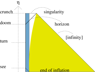
Figure 6: Even a weak perturbation will eventually go nonlinear, but there is plenty of time to avoid getting trapped in the collapse. This conformal diagram shows an exact solution constructed with the help of Birkhoff’s theorem. The blue region is a small portion of a closed universe (the polar cap of the three-sphere). Because its curvature radius is much larger than its size, it represents only a slightly overdense region embedded in a flat universe. The world volume of the unperturbed dust particles is shown in yellow. The white region is vacuous and is a portion of the Schwarzschild solution. It develops as the overdense region decouples from the ambient expansion. The perturbation is first fully seen at $\eta_{\rm see}$. It goes nonlinear much later, at $\eta_{\rm turn}$. Only at $\eta_{\rm doom}$ does the inert observer enter a black hole.

For small perturbations (Fig. 6), we thus see that the small parameter ${\cal P}_{\cal R}$ leads to large separations between $\eta_{\rm see}$, the time when the perturbation is first detected; $\eta_{\rm turn}$, the time when it becomes nonlinear; and finally, $\eta_{\rm doom}$, the time when black hole forms and the singularity is near. This leaves an observer plenty of time for escape from the overdense region, by moving to an underdense region after detecting a perturbation that would eventually enclose him in a black hole.

However, for larger perturbations, the separation of timescales shrinks. As longer wavelengths enter the horizon, there is less and less time for the observer to react and move to safety. Overdense perturbations of order one are lethal: For ${\cal P}_{\cal R}\sim 1$,

$$\eta_{\rm doom}\lesssim\eta_{\rm see}~{}.$$ (26)

By the time the observer can measure the curvature, he is already engulfed in a black hole and doomed to crunch. An example is shown in Fig. 7.

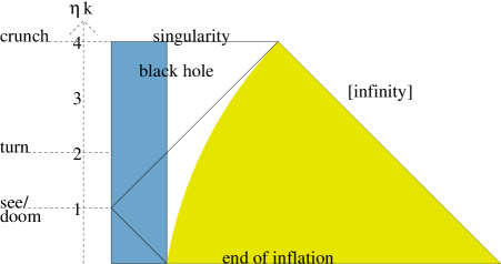
Figure 7: A strong perturbation catches the observer unaware (compare to Fig. 1). This conformal diagram shows another exact solution, but this time we keep half of the three-sphere of the closed universe (blue). This represents a strong perturbation because its size is comparable to its curvature radius. The observer can see the overdense region only as he is already falling into the black hole it forms.

Of course, not every perturbation is overdense; at any given time, it is just as likely that the next fluctuation to become visible will be underdense. But from the perspective of a local observer, one overdense perturbation is enough to cause a singularity. As the deformations of the metric due to inflaton field fluctuations become larger, there will eventually be an overdense fluctuation that will engulf the observer in a black hole.

IV False vacuum eternal inflation

We will begin this section by reviewing the conventional global description of FVEI. Next, we will describe the experience of a typical observer, and identify which aspects of the global description are unobservable. We find that observers who exit FVEI into a zero cosmological constant vacuum experience an open exapanding FRW universe. The presence of asymptotic regions with $\Lambda=0$ sharply distinguishes FVEI from SREI. We will argue that the inevitable collisions between true vacuum bubbles do not lead to gravitational collapse on large scales, so the asymptotic $\Lambda=0$ regions persist even after collisions are taken into account. We will support our claim by finding an exact solution describing the collision of two true vacuum bubbles. Furthermore, an infinite number of bubble collisions are contained within the horizon of an observer who exits to $\Lambda=0$.

IV.1 Conventional global description

The starting point for the global description of FVEI is the global de Sitter geometry associated with a metastable vacuum. Decay occurs by bubble nucleation, as described by Coleman and de Luccia CDL . Typically the new vacuum has lower cosmological constant (otherwise, interestingly, it cannot really be represented globally as a nucleation event in a background geometry). The bubble expands into the ambient de Sitter space, asymptotically approaching the speed of light. However, because the de Sitter space is itself expanding, it is not completely eaten by the bubble.

Eventually an infinite number of bubbles will nucleate, eating all of the comoving volume. However, the proper volume of each of the false vacua continues to grow. Vacua with $\Lambda\leq 0$ do not decay further and are called terminal. As described by Guth and Weinberg GutWei83 , a given bubble of true vacuum eventually collides with an infinite number of other bubbles. However, in the regime where inflation is eternal, the true vacuum regions form disconnected islands in the sea of false vacuum. Each island consists of an infinite number of bubbles, and there are an infinite number of islands.

A Penrose diagram of the global geometry is shown in Fig. 1. As discussed in Sec. II, this geometry cannot be constructed from initial conditions without appealing to an infinite number of causally disconnected observers.

IV.2 The fate of a generic observer

Just like in SREI, for any given worldline, inflation will not be eternal. The worldline will simply experience a sequence of tunneling events (typically decreasing the cosmological constant). If there are terminal vacua, it will end up in one after a finite time.

Thus, no single observer can see the complicated fractal global geometry described above. Observers who end up in a region with negative cosmological constant experience a big crunch within a time set by the curvature of the AdS space (see for example BJ ).

Observers in $\Lambda=0$ regions are much luckier. As the solution below shows, they find themselves in an expanding open FRW universe. Depending on the details, gravitational collapse can occur on short length scales. However, on sufficiently large length scales the curvature dominates and collapse cannot occur.

We describe the solution in some detail because we will need it in order to analyze bubble collisions in the following section. We confine ourselves to the thin wall approximation for simplicity, but indicate which features persist beyond this approximation.

The single bubble solution consists of a region of true vacuum surrounded by a domain wall, with false vacuum outside. Inside the domain wall, the spacetime is approximately empty, so the geometry is simply a region of Minkowski space glued across the thin domain wall to a portion of de Sitter space. The domain wall is a hyperboloid, whose worldvolume describes a three-dimensional de Sitter spacetime. Its curvature radius is $r_{0}$, where $r_{0}$ is determined by the tension $\sigma$ of the domain wall and the ($4$-dimensional) de Sitter radius $R$,

$$r_{0}={8\pi\sigma R^{2}\over(4\pi\sigma R)^{2}+1}~{}.$$ (27)

In the flat spacetime enclosed by the hyperboloid, the position of the domain wall satisfies

$$X_{\mu}X^{\mu}=-r_{0}^{2}~{},$$ (28)

where $X_{\mu}$ are the standard Minkowski coordinates. The wall expands from a minimum radius $r_{0}$, at $X_{0}=0$, to infinite size as $X_{0}\to\pm\infty$. To describe the motion of the domain wall from the de Sitter side, it is simplest to embed de Sitter space in $5$-dimensional Minkowski space as the surface

$$X_{\mu}X^{\mu}=-R^{2},~{}~{}~{}~{}~{}\mu=0,1,...,4$$ (29)

The domain wall is the intersection of the de Sitter space with the plane

$$X_{4}=(R^{2}-r_{0}^{2})^{1/2}.$$ (30)

The part of the space farther from the origin than the plane is discarded and replaced by the piece of flat space described above. An embedding picture of the solution is shown in figure 8.

Figure 8: The Coleman-De Luccia bounce geometry, as an embedding in Minkowski space. The flat piece has zero cosmological constant, while the curved piece has positive cosmological constant. A domain wall separates the two regions.

The solution is invariant under the symmetry group of the hyperboloid, $SO(1,3)$. On the de Sitter side, the full $SO(1,4)$ de Sitter symmetry is broken down to those boosts and rotations which leave $X_{4}$ unchanged. On the Minkowski side, the symmetry arises because the domain wall picks out an origin, breaking translation invariance while preserving the Lorentz group. The surviving $SO(1,3)$ symmetry is not an artifact of the thin wall approximation. It is present in the full solution.

One can write the metric in the flat space region in coordinates adapted to the symmetry,

$$ds^{2}=-dt^{2}+a(t)^{2}dH_{3}^{2}$$ (31)

In the thin wall approximation, $a(t)=t$ and these coordinates simply cover a piece of Minkowski space with hyperbolic time slices. Beyond the thin wall approximation, the $SO(1,3)$ symmetry which acts on $H_{3}$ is still present, but the scale factor changes. Beyond the thin wall approximation, a uniform energy density is present on the spatial slices, so the spacetime is an open expanding FRW universe.

IV.3 Bubble collisions

This picture is complicated by collisions with other true vacuum bubbles. However, we will now argue that they do not alter the conclusion that gravitational collapse stops after curvature domination. For this purpose, we will present an exact solution describing the collision of two bubbles of the same $\Lambda=0$ vacuum.

We will assume that all of the energy in the domain walls is converted to dust upon colliding. Since dust is generally more eager to collapse than any other type of matter, we expect that our conclusion extends to more general collisions.

We can use the de Sitter symmetries to make both bubbles time symmetric with respect to the global de Sitter time. Then in the embedding picture, each bubble is characterized by picking out a plane which is parallel to the $X_{0}$ axis. (In the one-bubble description above, we chose the plane $X_{4}=\sqrt{R^{2}-r_{0}^{2}}$.) The whole embedding picture is then the de Sitter hyperboloid cut by two planes. At $X_{0}=0$, the two bubbles are separated by a region of false vacuum, but as they grow they will collide. The surface along which they collide is a $2$-dimensional surface defined by the intersection of the de Sitter hyperboloid with the two planes: a spacelike 2-hyperboloid. When the true vacuum bubbles collide, the energy in the domain walls is converted to dust, and we will need a new solution to describe this part of the evolution. The two-bubble geometry preserves $SO(1,2)$ symmetry out of the original $SO(1,4)$ symmetry, because picking out the two planes is picking out two special directions. Rotations and boosts which leave the two special directions invariant are still symmetries of the problem.

We now construct a solution with the appropriate $SO(1,2)$ symmetry which consists of two flat spaces connected across a wall of dust. Since in the full solution dust is formed when the domain walls annihilate, we will need to use only a piece of this solution. The solution will be similar to the more familiar VIS solution in that it will consist of two spatially compact (in the Minkowski time slicing) regions of flat space joined across a wall of dust. Everything expands as time goes on.

We choose the $SO(1,2)$ symmetry to act on the coordinates $X_{0},X_{1},X_{2}$. To preserve the symmetry, the solution should only depend on the invariant interval $X_{0}^{2}-X_{1}^{2}-X_{2}^{2}$, and not on the coordinates separately. Defining a coordinate $\tau$ to be the proper time along the worldline of a dust particle, the wall will be described by two functions

$$X_{0}^{2}-X_{1}^{2}-X_{2}^{2} =f_{1}(\tau)$$ (32)

$$X_{3} =f_{2}(\tau)$$ (33)

The motion of the wall is determined by the Israel junction condition,

$$K_{ab}-h_{ab}K=8\pi T_{ab}$$ (34)

where $K_{ab}$ is the extrinsic curvature of the wall, $h_{ab}$ is the induced metric on the wall, $K$ is the trace of $K_{ab}$, and $T_{ab}$ is the stress tensor of the wall, which in our case should have a form appropriate for dust.

The solution is

$$X_{0}^{2}-X_{1}^{2}-X_{2}^{2} = \tau^{2}-L^{2}$$ (35)

$$X_{3} = b\pm L\cosh^{-1}({\tau\over L}).$$ (36)

Here $b$ is an arbitrary shift in the choice of origin and $L$ is a parameter which depends on the energy of the colliding domain walls. We can eliminate $\tau$ to find a single equation for the motion of the dust,

$$X_{0}^{2}-X_{1}^{2}-X_{2}^{2}=L^{2}\sinh^{2}\left({X_{3}-b\over L}\right)$$ (37)

The intrinsic geometry of the dust is given by

$$ds^{2}=-d\tau^{2}+(\tau^{2}-L^{2})dH_{2}^{2}$$ (38)

It is straightforward but tedious to check that this solution indeed satisfies the appropriate junction conditions for dust. The dust solution has a singularity at $\tau=L$; since we will only use part of the dust solution, this singularity will not concern us.

Now we need to patch the dust solution onto the domain wall solution to get our full solution. As noted above, the two true vacuum bubbles collide on a spacelike 2-hyperboloid, so it is along such a hyperboloid that we should match onto the dust solution. In the dust solution, the plane $X_{3}=constant$ intersects the wall of dust in a 2-hyperboloid.

To match, we require the radius of curvature of the $2$-hyperboloid to be equal to the radius of curvature $R_{H}$ along which the domain walls collide,

$$\tau_{0}^{2}-L^{2}=R_{H}^{2}$$ (39)

We also need energy conservation in the conversion of domain walls to dust. The junction condition relates the energy density to the parameters in the metric. To match, at the time the dust is created its energy should equal the center of mass energy $\rho_{0}$ of the domain wall collision,

$$\rho_{0}={L\over 2\pi(\tau_{0}^{2}-L^{2})}$$ (40)

Combining these equations, we solve for the parameters of the dust solution in terms of the parameters of the collision,

$$L = 2\pi R_{H}^{2}\rho_{0}$$ (41)

$$\tau_{0} = R_{H}\sqrt{1+(2\pi R_{H}\rho_{0})^{2}}$$ (42)

Let us summarize the entire solution, focusing on an observer at the center of one of the true vacuum bubbles. If there were just one true vacuum bubble, such an observer would see true vacuum out to a domain wall described by

$$X_{\mu}X^{\mu}=-r_{0}^{2}~{},$$ (43)

and false vacuum on the other side of the domain wall. Adding another bubble means that we replace part of the domain wall with dust. We can choose coordinates so that the part of the domain wall replaced by dust is the region with $X_{3}>a$. In the region it exists, the dust is described by Eq. (37). Given a collision which occurs along a $2$-hyperboloid with curvature radius $R_{H}$ and with center of mass energy $\rho_{0}$, the parameters in the solution are

$$L = 2\pi R_{H}^{2}\rho_{0}$$ (44)

$$a = \sqrt{r_{0}^{2}+R_{H}^{2}}$$ (45)

$$b = a-L\sinh^{-1}(R_{H}/L)$$ (46)

Passing through the wall of dust leads not to a region of false vacuum, but rather to another identical region of true vacuum.

The motion of individual dust particles obeys

$$X_{1} = \tanh\gamma\sin\phi~{}X_{0}~{},$$

$$X_{2} = \tanh\gamma\cos\phi~{}X_{0}~{},$$ (47)

$$X_{3} = b+L\sinh^{-1}\left(\frac{X_{0}}{L\cosh\gamma}\right)~{},$$

where $\gamma$ and $\phi$ label the worldline. Their asymptotic velocity is given by

$$\dot{X_{1}} =\tanh\gamma\sin\phi$$

$$\dot{X_{2}} =\tanh\gamma\cos\phi$$ (48)

$$\dot{X_{3}} ={1\over\sqrt{\cosh^{2}\gamma+\left({X_{0}\over L}\right)^{2}}}\to 0$$

where overdot signifies the derivative with respect to the Minkowski time $X_{0}$.

This shows that the dust particles are asymptotically moving away from each other with a relative velocity which depends on their location. As a result, the dust is not susceptible to gravitational collapse on large scales.

To understand the effect of the wall of dust on the open FRW universe present in the single bubble solution, it is helpful to rewrite the motion of the dust wall in coordinates suited to the open slicing, as well as to the symmetries preserved by the two-bubble solution. We write the metric in the form

$$ds^{2}=-dt^{2}+t^{2}dH_{3}^{2}\ ,$$ (49)

with the metric on the 3-hyperboloid in the form

$$dH_{3}^{2}=d\chi^{2}+\cosh^{2}\chi dH_{2}^{2}\ .$$ (50)

The $SO(1,2)$ symmetry of the solution is realized on the 2-hyperboloid. In these coordinates, at late times the dust wall obeys

$$\sinh\chi\approx{L\over t}\log\left({2t\over L}\right)\to 0\ .$$ (51)

On a given time slice, the spatial geometry consists of a piece of a 3-hyperboloid glued across a wall of dust to another copy of itself. The situation is most easily pictured by suppressing one dimension and using the Poincare disk representation of the hyperbolic plane, as shown in figures 9 and 10.

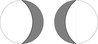
Figure 9: A constant time slice of the two-bubble solution. The spatial geometry consists of two 3-hyperboloids glued across a wall of dust to each other. Here the 3-hyperboloids are pictured, with one dimension suppressed, in the Poincare disk representation. The two disks are to be glued along the dust wall (heavy line), and the shaded regions are to be thrown away.

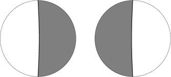
Figure 10: At late time, the wall of dust moves to the center of the hyperboloids. In this limit, the geometry reverts to one hyperboloid. Physically, this occurs because the dust has diluted and no longer causes a discontinuity in the geometry across the wall. Again, the shaded regions are to be thrown away and the two sides glued along the heavy line.

As seen in the above equation, at late times $\chi\to 0$. The surface $\chi=0$ is the diameter of the Poincare disk. Figure 9 shows the dust wall at a finite value of $\chi$, while figure 10 shows a later time, with the dust wall approaching $\chi=0$. Asymptotically, the two disks glue smoothly together into a single hyperboloid, so in this sense the open FRW geometry of the one-bubble solution is not destroyed by bubble collisions. However, note that although on the Poincare disk the dust wall approaches the center, the proper distance from an observer at the center ($X_{1}=X_{2}=X_{3}=0$) and the wall of dust grows to infinity, as is clear from (37). It approaches the center of the disk because the distance from the origin to the dust wall grows slower than the radius of curvature of the hyperboloid.

We have described the domain wall collision in a frame where the two bubbles of true vacuum are symmetric. A generic observer will typically see one of the bubbles nucleated long before the other, and hence much bigger than the other. Let us focus on an observer at the center of the biggest bubble (the “central observer”), keeping in mind that many observers can be brought to the same position by using the de Sitter symmetries. The central observer does not see the bubble collision occur in the center of mass frame; since his bubble has had much longer to expand, its domain wall is moving much faster than the domain wall of the smaller bubble.

To be precise, the central observer is related to the symmetric observer by a boost in the $X_{3}$ direction. To make the bubbles very asymmetrical requires a large boost. Now, instead of the wall of dust coming to rest at late times, as it did in the symmetric observer’s frame, it moves away from the central observer with a finite asymptotic velocity determined by the boost. This is shown in figure 11.

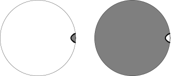
Figure 11: A typical observer sees a boosted version of the previous figure, with the dust wall asymptotically moving away at a finite velocity.

Recall that an infinite number of bubbles will eventually collide with the “central” bubble. These bubbles will collide with larger and larger boosts. The overall picture is of a central observer looking out at the night sky, seeing walls of dust moving away with bigger and bigger redshift. Gravitational collapse does not occur.

Acknowledgements

We would like to thank M. Kleban and L. Susskind for discussions. This work was supported by the Berkeley Center for Theoretical Physics, by a CAREER grant of the National Science Foundation, and by DOE grant DE-AC03-76SF00098.

Appendix A Slow-roll inflation and linear perturbations

In this appendix, we summarize slow-roll inflation and the production of perturbations of the spatial curvature. For a more detailed review, see Ref. LidLyt93 , whose notation we mostly follow.

A.1 The flat FRW universe

We work in the framework of a large, homogeneous, isotropic cosmology: the flat FRW universe. This is appropriate, assuming that inflation lasts slightly longer than necessary to explain the flatness of the observable universe.

The unperturbed metric is given by

$$ds^{2}=-dt^{2}+a(t)^{2}(dx^{2}+dy^{2}+dz^{2})~{}.$$ (52)

The scale factor $a$ satisfies the Friedmann equation,

$$H^{2}=\frac{8\pi}{3}\rho~{},$$ (53)

and the Raychaudhuri equation,

$$\dot{H}=-H^{2}-\frac{4\pi}{3}(\rho+3p)~{}.$$ (54)

The Hubble parameter $H$ is given by $\dot{a}/a$, $\rho$ is the density, and $p$ is the pressure of matter.

The apparent horizon is the hypersurface on which the past lightcones centered at $\mathbf{x}=0$ have maximal area (vanishing expansion) RMP . It is located at

$$ax=H^{-1}~{}.$$ (55)

Light-rays satisfy $dt/a=\pm dx$.

In a universe dominated by matter with equation of state $p=w\rho$, with $w\in(-1,1]$ a constant, the scale factor and density obey

$$a=t^{2/(3+3w)}~{},~{}~{}~{}\rho=\rho_{0}a^{-3-3w}~{}.$$ (56)

A cosmological constant, $w=-1$, yields de Sitter space (in the flat slicing):

$$a=e^{Ht}~{},~{}~{}~{}\rho=\frac{3H^{2}}{8\pi}=\mbox{const}~{}.$$ (57)

In this case the apparent horizon is light-like ($dt/a=-dx$) and coincides with a cosmological event horizon.

A.2 Inflation

For simplicity, we will consider only inflationary models driven by a single scalar field, $\phi$, with potential $V(\phi)$. Its equation of motion is

$$\ddot{\phi}+3H\dot{\phi}=-V^{\prime}(\phi)~{}.$$ (58)

The energy density and pressure are given by

$$\rho=V+\frac{1}{2}\dot{\phi}^{2}~{},~{}~{}p=-V+\frac{1}{2}\dot{\phi}^{2}~{}.$$ (59)

The Friedmann equations imply

$$\dot{H}=-4\pi\dot{\phi}^{2}$$ (60)

We assume the slow-roll conditions $\epsilon\ll 1$ and $|\eta|\ll 1$, where

$$\epsilon = \frac{1}{16\pi}\left(\frac{V^{\prime}}{V}\right)^{2}~{},$$ (61)

$$\eta = \frac{1}{8\pi}\frac{V^{\prime\prime}}{V}~{}.$$ (62)

The $\ddot{\phi}$ term in Eq. (58) can then be neglected, and we have

$$\dot{\phi}=-\frac{V^{\prime}}{3H}~{}.$$ (63)

That is, the motion of $\phi$ in its potential is overdamped. Moreover, we have $\dot{\phi}^{2}\ll V$ in Eq. (59), so

$$H^{2}=\frac{8\pi}{3}V$$ (64)

by the Friedmann equation (53).

Because $p\approx-\rho$ ($w\approx-1$), the evolution is similar to de Sitter space,

$$a(t)=\exp\int H(t)dt~{},\\$$ (65)

except that the Hubble parameter slowly decreases as $\phi$ rolls down. The above equations imply in particular that $\dot{H}/H^{2}<0$, $|\dot{H}/H^{2}|\ll 1$. Hence $H$ changes only by a small fraction over one Hubble time, $H^{-1}$, slowly increasing the size of the apparent horizon. From Eq. (55) one finds that the apparent horizon is (barely) timelike, satisfying

$$\frac{dt/a}{dx}=-\left(1+\frac{\dot{H}}{H^{2}}\right)^{-1}~{}.$$ (66)

A.3 Fluctuations of the inflaton

Density perturbations arise from quantum fluctuations of the inflaton field. Perturbing Eq. (58), one obtains Muk85 ; LidLyt93

$$\ddot{\phi_{\mathbf{k}}}+3H\dot{\phi_{\mathbf{k}}}+\left(\frac{k}{a}\right)^{2}\phi_{\mathbf{k}}=0~{},$$ (67)

where $\phi_{\mathbf{k}}$ is the Fourier transform of the field perturbation $\delta\phi$:

$$\delta\phi({\mathbf{x}},t)=(2\pi)^{-3}\int d^{3}{\mathbf{k}}\,\phi_{\mathbf{k}}(t)\,e^{i{\mathbf{k}}{\mathbf{x}}}~{}.$$ (68)

Note that ${\mathbf{x}}$ is a comoving coordinate. Hence, its conjugate, ${\mathbf{k}}$, is a comoving momentum. Physical scales are given by $a{\mathbf{x}}$ and ${\mathbf{k}}/a$.

Canonical quantization yields

$$\hat{\phi}_{\mathbf{k}}(t)=f_{k}(t)\hat{a}_{\mathbf{k}}+f^{*}_{-k}(t)\hat{a}^{\dagger}_{-\mathbf{k}}$$ (69)

where the creation and annihilation operators satisfy

$$[\hat{a}_{\mathbf{k}_{1}},\hat{a}^{\dagger}_{\mathbf{k}_{2}}]=(2\pi)^{3}\delta^{3}({\mathbf{k}_{1}}-{\mathbf{k}_{2}})~{},$$ (70)

and

$$f_{k}(t)=\frac{H}{(2k^{3})^{1/2}}\left(i+\frac{k}{aH}\right)e^{ik/aH}$$ (71)

is a solution to Eq. (67) which is positive frequency at early times. At very early times, the wavelength $a/k$ is much smaller than the curvature radius, and one expects the field to be in the vacuum:

$$\hat{a}_{\mathbf{k}}|0\rangle=0~{}.$$ (72)

As long as they are inside the horizon, the modes oscillate much like those of a scalar field in Minkowski space. After exiting the horizon, the modes freeze but continue expanding, so they contain more and more quanta. If the number of quanta is much greater than one, the field can be probed without altering the amplitude much. Let us assume, perhaps optimistically, that a stable, non-destructive measurement becomes possible when the mode has expanded by a couple of e-foldings after exit, when it is about a factor of $N_{\rm freeze}\approx 10$ larger than the horizon.

The corresponding “freezing surface” satisfies $ax=N_{\rm freeze}H^{-1}$. Its conformal slope is $1/N_{\rm freeze}$ times the slope of the apparent horizon, given in Eq. (66):

$$\frac{dt/a}{dx}=-\frac{1}{N_{\rm freeze}}\left(1+\frac{\dot{H}}{H^{2}}\right)^{-1}~{}.$$ (73)

Since $N_{\rm freeze}-1$ is not small, and since $\dot{H}/H^{2}\ll 1$, we have $|\frac{dt/a}{dx}|<1$.

This shows that the freezing surface is spacelike and becomes visible only after inflation ends (Fig. 12).

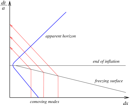
Figure 12: The hypersurface where inflationary modes freeze out is spacelike. Hence, frozen modes can be measured only after inflation has ended.

The expectation value of the Fourier amplitudes is given by

$$\langle 0|\hat{\phi}_{\mathbf{k}}\hat{\phi}_{-{\mathbf{k}}}|0\rangle=|f_{k}(t)|^{2}~{}.$$ (74)

After the mode exits the horizon ($k/a<H$), the first term in Eq. (71) becomes dominant and it ceases to oscillate. Then

$$\langle 0|\hat{\phi}_{\mathbf{k}}\hat{\phi}_{-{\mathbf{k}}}|0\rangle=\frac{H^{2}}{2k^{3}}~{}.$$ (75)

The fluctuations are Gaussian, i.e., the phases of the Fourier coefficients are random. In position space, the field perturbation is therefore given by the sum of the squared amplitudes:

$$\langle 0|\delta\phi(x)^{2}|0\rangle=\frac{1}{(2\pi)^{3}}\int d^{3}k\,|f_{k}|^{2}~{}.$$ (76)

In practice one does not measure a single mode, but a range of wavelengths and orientations (say, all momenta with magnitude between $k$ and $ek$). The resulting perturbation is captured by the power spectrum, ${\cal P}_{\phi}(k)$, defined by

$$\langle 0|\delta\phi({\mathbf{x}})\delta\phi({\mathbf{x+r}})|0\rangle=\int_{0}^{\infty}{dk\over k}{\sin(kr)\over kr}{\cal P}_{\phi}(k)\ .$$ (77)

The power spectrum for any other perturbation $\beta$ is defined analogously. The power spectrum is simply related to the mode functions $f_{k}$,

$${\cal P}_{\phi}(k)=\frac{k^{3}}{2\pi^{2}}|f_{k}|^{2}~{}.$$ (78)

After horizon exit (for $Ha/k>1$), a typical fluctuation is $H/2\pi$:

$${\cal P}_{\phi}=\left(\frac{H}{2\pi}\right)^{2}~{}.$$ (79)

We are particularly interested in the behavior of the fluctuations on the Hubble scale. The inflaton fluctuation averaged over the Hubble scale is given by

$$\delta\phi_{H}(t)=(2\pi)^{-3}\int d^{3}{\mathbf{k}}\ \sigma_{t}(k)\phi_{k}(t)$$ (80)

where $\sigma_{t}(k)$ is a smearing function appropriate to averaging over one Hubble volume at time $t$. A natural quantity to compute which captures the buildup of the fluctuations on the Hubble scale is

$$\langle\left[\delta\phi_{H}(t_{2})-\delta\phi_{H}(t_{1})\right]^{2}\rangle~{}.$$ (81)

Using the definition of $\delta\phi_{H}$, we find

$$\langle\left[\delta\phi_{H}(t_{2})-\delta\phi_{H}(t_{1})\right]^{2}\rangle=$$

$$\langle\left[(2\pi)^{-3}\int d^{3}{\mathbf{k}}\ \sigma_{t_{2}}(k)\hat{\phi}_{\mathbf{k}}(t_{2})-\sigma_{t_{1}}(k)\hat{\phi}_{\mathbf{k}}(t_{1})\right]^{2}\rangle$$ (82)

Using momentum conservation, we can bring the square inside the integral. Also, we decompose the field in terms of creation and annihilation operators as in equation (69). We find

$$\langle\left[\delta\phi_{H}(t_{2})-\delta\phi_{H}(t_{1})\right]^{2}\rangle=$$

$$(2\pi)^{-3}\int d^{3}{\mathbf{k}}\ \left|\sigma_{t_{2}}(k)f_{k}(t_{2})-\sigma_{t_{1}}(k)f_{k}(t_{1})\right|^{2}\ .$$ (83)

We consider a particularly simple smearing function whose value is 1 for modes with wavelength longer than the Hubble scale and 0 otherwise,

$$\sigma_{t}(k)=\begin{cases}1\ \ &{\rm for}\ k<a(t)H\\ 0&{\rm for}\ k>a(t)H\end{cases}$$ (84)

Because the position space smearing function should integrate to 1, the momentum space smearing function should satisfy $\sigma_{t}(k=0)=1$. Our smearing function has this property. Incidentally, this property guarantees that the quantity we are calculating is free of the infrared divergences which appear in many computations of the inflaton fluctuations. Continuing with our calculation, we note that since the smearing function only has support on wavelengths larger than the Hubble radius, we can approximate

$$f_{k}(t)\approx iH/\sqrt{2k^{3}}$$ (85)

in equation (83). (In fact, this approximation becomes good for modes well outside the horizon. We will focus on the buildup of fluctuations over many efoldings, and we will see that the dominant contribution comes from modes well outside the horizon.) With this approximation, the integral simplifies to

$$\langle\left[\delta\phi_{H}(t_{2})-\delta\phi_{H}(t_{1})\right]^{2}\rangle=$$

$${1\over 2\pi^{2}}\int_{0}^{\infty}dk\ k^{2}\left|\sigma_{t_{2}}(k)-\sigma_{t_{1}}(k)\right|^{2}{H^{2}\over 2k^{3}}\ .$$ (86)

Using the definition of the smearing function $\sigma$, the integral becomes

$$\langle\left[\delta\phi_{H}(t_{2})-\delta\phi_{H}(t_{1})\right]^{2}\rangle$$

$$=\left({H\over 2\pi}\right)^{2}\int_{a(t_{1})H}^{a(t_{2})H}{dk\over k}$$

$$=\left({H\over 2\pi}\right)^{2}\log{a(t_{2})\over a(t_{1})}\ .$$ (87)

The logarithmic integral above receives equal weight from every efolding. Since we are interested in integrating over a large number of efoldings, it is dominated by modes well outside the horizon, so our approximation (85) is justified. We can rewrite our answer in a more suggestive way,

$$\langle\left[\delta\phi_{H}(t_{2})-\delta\phi_{H}(t_{1})\right]^{2}\rangle=\left({H\over 2\pi}\right)^{2}Ht$$ (88)

This formula is correct in the limit that the number of efoldings, $Ht$, is large. Furthermore, since the action is quadratic, the fluctuations will be gaussian. The above formula makes clear that the variance of the gaussian grows linearly with time, just as for a random walk. One way to think about it is that the inflaton field on the Hubble scale is performing a random walk, taking a step of size $H/2\pi$ every Hubble time.

A.4 Curvature perturbations

Next, let us discuss how the perturbations of the inflaton field lead to perturbations of the metric. In semiclassical gravity, the stress tensor entering the Einstein equation is the expectation value of the stress tensor of quantum field theory:

$$R_{ab}-\frac{1}{2}Rg_{ab}=8\pi\langle T_{ab}\rangle~{}.$$ (89)

In this framework the fluctuations computed above would be irrelevant, since $\langle\delta\phi\rangle=0$. The metric would remain unperturbed, because the expectation value of the quantum field remains unperturbed at linear order.

If quantum fluctuations are to shape the metric, one must go somewhat beyond the framework of semiclassical gravity. The point is that if the field is measured, it takes on a typical value in the range where its wavefunction has support. A typical value will deviate from the expectation value by approximately $\pm\delta\phi$. But using a typical value would not be appropriate for the ultraviolet fluctuations of fields in flat space. We must therefore justify this approach carefully for the case of frozen modes of the inflaton field.

First, consider high frequency modes of $\phi$. They are shorter than the Hubble length, $a/k<H^{-1}$, and behave as in flat space. By Eq. (78), the power spectrum in this regime is

$${\cal P}_{\phi}=\frac{k^{2}}{2a^{2}}=\frac{p^{2}}{2}$$ (90)

Thus a typical fluctuation is of order $p$, the physical momentum, which is large in the ultraviolet. These fluctuations would be seen if such modes were measured, that is, if the field interacted with probes sufficiently energetic to resolve small distances. Even then, they would not be stable, in the sense that the field would continue to oscillate. The interaction will have imparted significant unknown momentum to the field, so that multiple measurements of the same range of modes would not be strongly correlated. Note that in the inflationary universe, no probes are available at very high energies, so presumably such interactions do not occur, and the quantum state of the inflaton field remains coherent.

Modes that are larger than the Hubble scale, however, decohere KiePol98 . They are probed by the environment (at least, by gravity). Thus, their quantum state becomes entangled with the environment. After tracing over unobservable environmental degrees of freedom, coherence is lost and a density matrix remains. Because the amplitude remains constant while the wavelength expands, each mode will contain a large number of quanta, and its state will not be significantly altered by interactions. Hence, the modes behave classically, drawn from the statistical sample described by the density matrix.

Now let us relate the perturbations of the inflaton field to deformations of the spatial metric. In the unperturbed spacetime, Eq. (52), the spatial metric is flat and the inflaton field is constant ($\delta\phi=0$) on any flat slice. With perturbations included, the backreaction on the metric is second order, so one can still consider flat slices, but with $\delta\phi\neq 0$. However, in order to evolve the effects of perturbations into the radiation and matter dominated eras, it is more convenient to work in the comoving gauge. This slicing is defined by the requirement that the momentum density of the cosmological fluid, $T_{0i}$, vanish. During inflation this means that $\delta\phi=0$ on comoving slices.

Therefore, comoving slices are slightly deformed relative to the flat slices, by a position-dependent time difference

$$\delta t({\mathbf{x}})=-\delta\phi({\mathbf{x}})/\dot{\phi}~{}.$$ (91)

The three-dimensional curvature will not vanish on a comoving slice. It is given by LytRio98

$${\cal R}({\mathbf{x}})=H\delta t({\mathbf{x}})~{},$$ (92)

where ${\cal R}$ is “sourced” by the three-dimensional curvature scalar:

$$-4\nabla^{2}{\cal R}=\mbox{}^{3}\!R~{}.$$ (93)

Note that ${\cal R}$ is dimensionless. Its physical significance is best understood by thinking of its Fourier transform

$${\cal R}_{\mathbf{k}}=\frac{1}{4}\frac{a^{2}}{k^{2}}\,\mbox{}^{3}\!R_{\mathbf{k}}~{}.$$ (94)

As above, one can define a power spectrum for ${\cal R}$, via

$$\langle{\cal R}({\mathbf{x}}){\cal R}(\mathbf{x+r})\rangle=\int_{0}^{\infty}{dk\over k}{\sin(kr)\over kr}{\cal P}_{\cal R}(k)\ .$$ (95)

If ${\cal P}_{\cal R}^{1/2}(k)\ll 1$, then the spatial geometry is nearly flat on the physical distance scale $a/k$. On the other hand, ${\cal P}_{\cal R}^{1/2}(k)\sim 1$ indicates that the spatial geometry is significantly curved on the physical distance scale $a/k$.

If pressure gradients are small, different regions in a weakly perturbed universe evolve independently. This leads to an important property of ${\cal P}_{\cal R}(k)$ LidLyt93 : it is time-independent as long as the pressure gradient remains negligible and the perturbations remain linear. This holds during conventional slow-roll inflation, and remains true when the mode is frozen outside the horizon. It also holds during matter domination since the pressure vanishes then. Thus ${\cal P}_{\cal R}(k)$ remains constant for all modes that re-enter after matter has begun to dominate. We are interested in large scales, so we will neglect the radiation dominated era. Then ${\cal R}_{k}$ is constant for all $k$, as long as perturbations are linear.

The curvature perturbation ${\cal R}$ is simply related to the density contrast

$$\delta\equiv\frac{\delta\rho}{\rho}$$ (96)

during the matter dominated era, through

$$\left(\frac{aH}{k}\right)^{2}\delta_{\mathbf{k}}=\frac{2}{5}{\cal R}_{\mathbf{k}}~{}.$$ (97)

The spectral index, $n$, is defined via

$$n-1=\frac{d\log{\cal P}_{\cal R}(k)}{d\log k}~{}.$$ (98)

Observables such as the temperature variations in the CMB can be computed from these quantities. However, in the context of the questions posed in this paper, it will serve clarity if we suppress the indirect routes by which aspects of the geometry of the universe are determined in practice. Instead we will pretend, optimistically, that we are able to measure directly the geometry of post-inflationary comoving three-surfaces—at least, the portions contained in our past lightcone.

We are now ready to combine results from the above discussion. From Eqs. (91) and (92) the spectrum of curvature perturbations is

$${\cal P}_{\cal R}^{1/2}(k)=\frac{H_{*}}{|\dot{\phi}_{*}|}{\cal P}_{\phi}^{1/2}(k)=\frac{H_{*}^{2}/2\pi}{V^{\prime}_{*}/3H_{*}}=\frac{H_{*}^{2}}{H_{*}^{\prime}}~{}.$$ (99)

The star indicates that quantities are to be evaluated at the time when $aH/k=1$, i.e., when the mode $k$ exits the horizon during inflation. This is just before the quantum state decoheres and becomes a classical perturbation of the comoving geometry. (Because both $H$ and $H^{\prime}$ change slowly, it does not matter whether they are evaluated a few Hubbles times too early.) Thereafter, inflation continues and the Hubble constant varies, but as explained above, the curvature perturbation remains constant.

References

- (1) S. Coleman and F. D. Luccia: Gravitational effects on and of vacuum decay. Phys. Rev. D 21, 3305 (1980).
- (2) A. H. Guth and E. J. Weinberg: Could the universe have recovered from a slow first-order phase transition?. Nucl. Phys. B212, 321 (1983).
- (3) A. Vilenkin: The birth of inflationary universes. Phys. Rev. D 27, 2848 (1983).
- (4) A. Linde: Eternal chaotic inflation. Mod. Phys. Lett. A1, 81 (1986).
- (5) A. G. Riess et al.: Observational evidence from supernovae for an accelerating universe and a cosmological constant. Astron. J. 116, 1009 (1998), astro-ph/9805201.
- (6) A. D. Sakharov: Cosmological transitions with a change in metric signature. Sov. Phys. JETP 60, 214 (1984).
- (7) S. Weinberg: Anthropic bound on the cosmological constant. Phys. Rev. Lett. 59, 2607 (1987).
- (8) R. Bousso and J. Polchinski: Quantization of four-form fluxes and dynamical neutralization of the cosmological constant. JHEP 06, 006 (2000), hep-th/0004134.
- (9) S. Kachru, R. Kallosh, A. Linde and S. P. Trivedi: De Sitter vacua in string theory. Phys. Rev. D 68, 046005 (2003), hep-th/0301240.
- (10) A. D. Linde: Particle physics and inflationary cosmology. Harwood, Chur, Switzerland (1990).
- (11) A. S. Goncharov, A. D. Linde and V. F. Mukhanov: The global structure of the inflationary universe. Int. J. Mod. Phys. A2, 561 (1987).
- (12) A. Linde, D. Linde and A. Mezhlumian: Nonperturbative amplifications of inhomogeneities in a self-reproducing universe. Phys. Rev. D 54, 2504 (1996), gr-qc/9601005.
- (13) L. Susskind, L. Thorlacius and J. Uglum: The stretched horizon and black hole complementarity. Phys. Rev. D 48, 3743 (1993), hep-th/9306069.
- (14) R. Bousso: Holographic probabilities in eternal inflation (2006), hep-th/0605263.
- (15) L. Dyson, M. Kleban and L. Susskind: Disturbing implications of a cosmological constant. JHEP 10, 011 (2002), hep-th/0208013.
- (16) N. Kaloper, M. Kleban and L. Sorbo: Observational implications of cosmological event horizons. Phys. Lett. B600, 7 (2004), astro-ph/0406099.
- (17) M. Schlosshauer: Decoherence, the measurement problem, and interpretations of quantum mechanics. Rev. Mod. Phys. 76, 1267 (2004), quant-ph/0312059.
- (18) S. Coleman and F. D. Luccia: Gravitational effects on and of vacuum decay. Phys. Rev. D 21, 3305 (1980).
- (19) T. Banks and M. Johnson: Regulating eternal inflation (2005), hep-th/0512141.
- (20) A. R. Liddle and D. H. Lyth: The cold dark matter density perturbation. Phys. Rept. 231, 1 (1993), astro-ph/9303019.
- (21) R. Bousso: The holographic principle. Rev. Mod. Phys. 74, 825 (2002), hep-th/0203101.
- (22) V. F. Mukhanov: Gravitational instability of the universe filled with a scalar field. JETP Lett. 41, 493 (1985).
- (23) C. Kiefer, D. Polarski and A. A. Starobinsky: Quantum-to-classical transition for fluctuations in the early universe. Int. J. Mod. Phys. D7, 455 (1998), gr-qc/9802003.
- (24) D. H. Lyth and A. Riotto: Particle physics models of inflation and the cosmological density perturbation. Phys. Rept. 314, 1 (1999), hep-ph/9807278.