Ricci flow and black holes

Abstract:

Gradient flow in a potential energy (or Euclidean action) landscape provides a natural set of paths connecting different saddle points. We apply this method to General Relativity, where gradient flow is Ricci flow, and focus on the example of 4-dimensional Euclidean gravity with boundary $S^{1}\times S^{2}$, representing the canonical ensemble for gravity in a box. At high temperature the action has three saddle points: hot flat space and a large and small black hole. Adding a time direction, these also give static 5-dimensional Kaluza-Klein solutions, whose potential energy equals the 4-dimensional action. The small black hole has a Gross-Perry-Yaffe-type negative mode, and is therefore unstable under Ricci flow. We numerically simulate the two flows seeded by this mode, finding that they lead to the large black hole and to hot flat space respectively, in the latter case via a topology-changing singularity. In the context of string theory these flows are world-sheet renormalization group trajectories. We also use them to construct a novel free energy diagram for the canonical ensemble.

1 Introduction and summary

Gradient flow is a powerful theoretical tool for exploring a system’s potential energy landscape, which has been applied in contexts ranging from biophysics to string theory. Similarly, it is sometimes useful to study gradient flow of a system’s action on its space of histories, for example in the context of the path integral formulation of quantum mechanics. (Like the path integral, the gradient flow will strictly speaking be well defined only in the Euclidean framework.)

The purpose of this paper is to investigate gradient flow, both of the potential energy and of the Euclidean action, in the context of General Relativity. Gradient flow of the Einstein-Hilbert action on the space of metrics on a given manifold is governed by the following equation:

$$\frac{\partial g_{\mu\nu}}{\partial\lambda}=-2R_{\mu\nu},$$ (1)

where $\lambda$ is the flow time. In the mathematical literature, the flow defined by equation (1) is known as Ricci flow, and in recent years has been the subject of intense study. It also arises in string theory as the one-loop approximation to the renormalization group (RG) flow of sigma models. Section 2 of this paper is devoted to a review of the basic properties of Ricci flow.

As our laboratory for the application of Ricci flow to gravity, we take one of the simplest systems that admits multiple saddle points: 4-dimensional pure gravity (without cosmological constant) in a spherical box of radius $R$, in the canonical ensemble at temperature $\beta^{-1}$. The path integral for this system involves all Euclidean metrics, on all topologies, with boundary $S^{1}_{\beta}\times S^{2}_{R}$. At high temperature there are three saddle points of the action: a large and a small black hole, and the product of $S^{1}_{\beta}$ with a flat 3-ball. The Lichnerowicz operators for the large black hole and hot flat space metrics are positive definite, whereas, as we show, the one for the small black hole has a single negative eigenvalue, analogous to that of Gross, Perry, and Yaffe (GPY) [1] in the asymptotically flat case. This indicates that the small black hole is truly a saddle point of the action, whereas the other two solutions are actually local minima (not counting Weyl fluctuations of the metric, which always decrease the action; these are dealt with in the path integral by rotating their contours of integration). GPY argued that, due to this negative mode, the small black hole serves as a bounce (or sphaleron) that allows the system to pass from one minimum to the other by thermal fluctuations. Furthermore, according to arguments given by Whiting and York [2], Whiting [3], Prestidge [4], and Reall [5], this negative mode is related to the local thermodynamic instability of the corresponding Lorentzian black hole.

We can also add a time direction to the system, and consider 5-dimensional Lorentzian gravity with boundary $\mathbf{R}\times S^{1}_{\beta}\times S^{2}_{R}$. Ignoring the Hamiltonian constraint (which in any case is automatically satisfied at the saddle points), the space of time-symmetric initial data is the space of Euclidean 4-metrics, and the potential energy is the 4-dimensional Euclidean action. The three saddle points give static solutions, which are reinterpreted in this context as large and small bubbles of nothing and the Kaluza-Klein vacuum, respectively. Their dynamical stability is controlled by the Lichnerowicz operators for the respective Euclidean 4-metrics, so the small bubble has a tachyon while the other two solutions are stable. Further details about both the Euclidean and the Lorentzian versions of this system are given in Section 3.

In both of the above contexts, Ricci flow describes gradient flow: of the potential energy in the 5-dimensional Lorentzian context, and of the action in the 4-dimensional Euclidean one. The small black hole’s negative mode indicates that it is unstable under Ricci flow. This raises the question of where the two flows that start at this saddle point, moving opposite ways along the unstable direction, ultimately end up. One guess would be that each flow asymptotes to one of the other two saddle points. Using numerical simulations we were able to confirm this guess; this is the main result of this paper. Ricci flow thus defines a unique path in the space of metrics connecting the small black hole to each of the other two saddle points. The one connecting the small black hole to hot flat space is particularly interesting, because at a finite flow time the metric passes through a localized topology-changing singularity (the metrics are otherwise smooth throughout the flows). The flows are described in detail in Section 4.

These flows have various applications. In the context of string theory, they represent world-sheet RG trajectories, with the small black hole as the ultraviolet fixed point and hot flat space and the large black hole as the infrared ones. It is interesting that they qualitatively mirror the time evolution of the Lorentzian small black hole perturbed by its thermodynamic instability, as it either evaporates or grows to become the large black hole. Quantitatively, however, the evolution is different, since at every point along the evaporation process the geometry remains Schwarzschild to a good approximation, whereas as we will see along the RG flows it does not.

RG flow is also often applied to the spatial part of a world-sheet theory as a technique for studying closed-string tachyons. Hence we may use the terminology of the 5-dimensional Lorentzian context and say that the small bubble of nothing (which has a tachyon, and therefore a relevant operator on the world-sheet) is the UV fixed point, and the large bubble and Kaluza-Klein vacuum are the IR fixed points. These flows are in accord with the arguments made in the paper [6], that the ADM energy of the target space should be lower in the IR than in the UV of a world-sheet RG flow. The full dynamical evolution of the unstable small bubble has been performed by Lehner and Sarbach [7, 8], and we may contrast this behavior with the RG flows. In the case where the small bubble initially expands, the dynamical simulations were consistent with the large stable bubble being the end state, although the simulations were not performed in a box and so saw only continued expansion. The more interesting case is initial collapse of the small bubble, which in RG flow goes to Kaluza-Klein flat space, but dynamically forms a Kaluza-Klein black string. Whilst this will indeed evaporate to flat space eventually, RG flow and classical dynamics clearly do not agree for this system. We attribute the difference to the fact that this flow involves a topology change, and whilst this may occur smoothly in RG flow, in the dynamical case cosmic censorship is expected to form a horizon to shield it.

Another application of our flows is in the Euclidean (thermal) context. The fact that Ricci flow is gradient flow means that, at any point along the flow, the action is stationary in the directions orthogonal to it. Hence in principle these directions can be integrated out to define an off-shell free energy; in a saddle point approximation this free energy is simply equal to the value of the action at that point on the curve. Thus, Ricci flow can be used to construct a new type of free energy diagram for this thermal system. This diagram, shown in figure 10, is discussed further in Section 5.

Although we studied the specific case of 4 dimensions, it seems likely that the flows are qualitatively similar in higher dimensions. Also, while we employed a simple box as our infrared regulator, our results would likely have been qualitatively unchanged had we instead included a negative cosmological constant and imposed asymptotically anti-de Sitter boundary conditions. It would be interesting to see whether they have physical implications in the context of the AdS-CFT correspondence, and we conclude the paper with a brief comment on this.

Ricci flow has previously been studied numerically in a variety of contexts. For example, a 2-dimensional flow asymptoting to the dilaton black hole was studied by Hori and Kapustin [9]. The formation of singularities in 3 dimensions was studied by Garfinkle and Isenberg [10, 11]. And Ricci flow was investigated as a numerical method for solving the Einstein equation on the 4-dimensional manifold K3 by the present authors [12]. However, as far as we know the flows we study in this paper are the first explicitly known that connect different saddle points of the action.

2 Ricci flow

Ricci flow is an analog of the heat equation for geometry, a diffusive process acting on the metric of a Riemannian manifold. In this section we define it, explain its basic mathematical properties, and describe how it appears in several different contexts in physics. Indeed, historically it was in physics that Ricci flow first made its appearance, in the work of Friedan [13] on the renormalization group for two-dimensional sigma models. It was subsequently introduced into mathematics by Hamilton [14] as a tool for studying the topology of manifolds. Among other things, he developed a program, recently brought to fruition by Perelman [15, 16], for proving Thurston’s geometrization conjecture concerning the classification of 3-manifolds (for reviews see [17, 18]). By now there is a very extensive literature (including a textbook [19]) on Ricci flow.

The material in this section is review, except the discussion of boundary conditions in subsection 2.2, which is new as far as we know.

2.1 Definition and basic properties

Let $M$ be a $D$-dimensional compact manifold, and $\mathcal{H}$ the space of Euclidean (i.e. positive definite) metrics $g_{\mu\nu}(x)$ on it (not the space of metrics modulo diffeomorphisms). Ricci flow is the first-order flow on $\mathcal{H}$, with respect to an auxiliary “time” variable $\lambda$, defined by

$$\frac{\partial g_{\mu\nu}(x,\lambda)}{\partial\lambda}=-2R_{\mu\nu}(x,\lambda).$$ (2)

The flow is obviously invariant under ($\lambda$-independent) diffeomorphisms of $M$. It is sometimes useful to consider the more general equation

$$\frac{\partial g_{\mu\nu}}{\partial\lambda}=-2R_{\mu\nu}+2\nabla_{(\mu}\xi_{\nu)},$$ (3)

where $\xi^{\nu}(x,\lambda)$ is some vector field. In fact, it’s easy to see that the solutions to equations (2) and (3) are the same, up to the diffeomorphism obtained by integrating $\xi^{\mu}$ with respect to $\lambda$. Thus the two equations describe different flows in $\mathcal{H}$, but the same flow in the quotient of $\mathcal{H}$ by diffeomorphisms of $M$.

In what sense is Ricci flow diffusive? Let us examine how a short-wavelength, small-amplitude perturbation of the metric evolves. If the wavelength is much shorter than the typical curvature radius of the manifold, then it is sufficient to expand about flat space. With $g_{\mu\nu}=\delta_{\mu\nu}+h_{\mu\nu}$, we find, to linear order,

$$\frac{\partial h_{\mu\nu}}{\partial\lambda}=\nabla^{2}h_{\mu\nu}+2\partial_{(\mu}v_{\nu)}+O(h^{2}),$$ (4)

where

$$v_{\nu}\equiv\frac{1}{2}\partial_{\nu}h_{\lambda\lambda}-\partial_{\lambda}h_{\lambda\nu}.$$ (5)

We see that the perturbation evolves according to the heat equation, accompanied by a small diffeomorphism. Just as with the scalar heat equation, we are restricted to Euclidean signature, since on a Lorentzian background the flow is infinitely unstable to modes with timelike momentum, and therefore ill defined.

How unique is Ricci flow? Suppose that we wish to define a flow equation for the metric that is local and diffeomorphism-invariant and that contains at most two second derivatives acting on the metric. There are only two terms we could add to the right-hand side of (2):

$$\frac{\partial g_{\mu\nu}}{\partial\lambda}=-2R_{\mu\nu}+\alpha Rg_{\mu\nu}+2\Lambda g_{\mu\nu}.$$ (7)

Because it contains no derivatives, the $\Lambda$ term does not change the behavior of short-wavelength perturbations, and therefore does not affect the locally diffusive nature of the flow. While it is useful when one is interested in flows that start or end on Einstein metrics with non-zero cosmological constant, in this paper we will set $\Lambda=0$ for simplicity. On the other hand, having a non-zero $\alpha$ changes the right-hand side of (4), adding the terms $\alpha(\partial_{\lambda}\partial_{\rho}h_{\lambda\rho}-\nabla^{2}h_{\lambda\lambda})\delta_{\mu\nu}$, which has the effect of making different polarizations diffuse at different rates. A given perturbation can be decomposed into a part obeying $\partial_{\lambda}\partial_{\rho}h_{\lambda\rho}-\nabla^{2}h_{\lambda\lambda}=0$, which evolves independently of $\alpha$, and a Weyl part (proportional to $\delta_{\mu\nu}$), which evolves with a diffusion constant $1-\alpha(D-1)$. In particular, unless $\alpha\leq 1/(D-1)$ the flow is ill defined. In this sense Ricci flow is singled out; as we will discuss below, the value $\alpha=0$ is also physically selected in the context of RG flow. It would be interesting to understand how general our results are for the other values of $\alpha$ for which the flow is well defined.

Now let us review the basic global properties of Ricci flow. The fixed points are obviously Ricci-flat metrics. The generalization of the linearization (4) to the case $g_{\mu\nu}=\hat{g}_{\mu\nu}+h_{\mu\nu}$, where $\hat{g}_{\mu\nu}$ is Ricci-flat, is

$$\frac{\partial h_{\mu\nu}}{\partial\lambda}=-\Delta_{\rm L}h_{\mu\nu}+2\nabla_{(\mu}v_{\nu)}+O(h^{2}),$$ (8)

where $v_{\nu}\equiv\frac{1}{2}\partial_{\nu}{h^{\lambda}}_{\lambda}-\nabla_{\lambda}{h^{\lambda}}_{\nu}$, and $\Delta_{\rm L}$ is the Lichnerowicz operator:

$$\Delta_{\rm L}h_{\mu\nu}\equiv-\nabla^{\lambda}\nabla_{\lambda}h_{\mu\nu}-2{{{R_{\mu}}^{\kappa}}_{\nu}}^{\lambda}h_{\kappa\lambda}$$ (9)

(everything is calculated with respect to the background metric $\hat{g}_{\mu\nu}$). The linear stability of the fixed point is thus determined by the existence of negative eigenvalues of $\Delta_{\rm L}$. ($\Delta_{\rm L}$ is non-negative on pure gauge modes, so any negative mode must be physical.) $\Delta_{\rm L}$ acts separately on Weyl ($h_{\mu\nu}(x)=\epsilon(x)\hat{g}_{\mu\nu}(x)$) and traceless (${h^{\mu}}_{\mu}(x)=0$) modes. For Weyl modes it reduces to minus the scalar Laplacian, which is non-negative on a compact manifold. On the other hand, for traceless modes the Riemann tensor acts as a “potential” on the manifold (in the sense of the Schrödinger equation), with regions of positive curvature corresponding to negative potential energy. The operator may therefore have a finite number of “bound states”, i.e. modes with negative eigenvalue.

Another important property of Ricci flow, obvious from the definition, is that regions (and, within a region, directions) with positive Ricci curvature tend to collapse. This can lead to the formation of curvature singularities in finite flow time. The simplest example is to start with the round metric on the $D$-sphere. We will see a more complicated example in the flows we study in this paper.

2.2 Boundaries

In Section 4 we will consider Ricci flow on a manifold with boundary. We should therefore consider what boundary conditions are required to render the flow well defined. Let us locally divide the coordinates into ones that are parallel ($x^{i}$) and normal ($x^{n}$) to the boundary. In general for a diffusive flow one should impose a single boundary condition (such as Dirichlet or Neumann) on any variable $f$ which is acted on by a second derivative normal to the boundary, i.e. where $\partial_{n}^{2}f$ appears, while for any variable acted on by fewer than two normal derivatives, no boundary condition should be imposed. In the Ricci tensor only the metric components along the boundary, $g_{ij}$, appear with two normal derivatives, so it is only on these that we should impose boundary conditions. For example, in the Dirichlet case we would fix the induced metric $\gamma_{ij}$ on the boundary, while in the Neumann case we would fix its extrinsic curvature $K_{ij}$ (the latter case is treated in the paper [21]). These are the same kinds of boundary conditions one can impose on the hyperbolic time evolution of general relativity.

In what follows, we will adopt Dirichlet boundary conditions. $\mathcal{H}$ is therefore defined as the space of Euclidean metrics on $M$ with a fixed induced metric $\gamma_{ij}$ on $\partial M$. An important technical point is that, with these boundary conditions, we cannot make the usual decomposition of perturbations into Weyl and traceless parts. Specifically, a perturbation whose component $h_{nn}$ doesn’t vanish at the boundary cannot be expressed as the sum of an allowed Weyl and an allowed traceless perturbation.

2.3 Ricci flow as gradient flow

The fixed points of Ricci flow, namely the Ricci-flat metrics, coincide for $D>2$ with the critical points of the Euclidean Einstein-Hilbert action,

$$S[g_{\mu\nu}(x)]=-\frac{1}{16\pi G_{\rm N}}\int_{M}\sqrt{g}R-\frac{1}{8\pi G_{\rm N}}\int_{\partial M}\sqrt{\gamma}K+S_{0}$$ (10)

($S_{0}$ is an arbitrary constant). This suggests that Ricci flow might be gradient flow of $S$. We will now show that this is the case.

Recall that the general gradient flow equation, on a space with coordinates $g^{A}$ and “energy” function $S$, is

$$\frac{dg^{A}(\lambda)}{d\lambda}=-G^{AB}\frac{\partial S}{\partial g^{B}}.$$ (11)

The inverse metric $G^{AB}$ is necessary to raise the index on the gradient. In our case $g^{A}$ is $g_{\mu\nu}(x)$, the index $A$ standing for both the point $x$ in $M$ and the component $\mu\nu$, and $S$ is the Einstein-Hilbert action. But what should we take for $G_{AB}$? The most general metric on $\mathcal{H}$ that is local and diffeomorphism-invariant (on $M$) and contains no derivatives is of the form

$$G^{(a)}_{AB}dg^{A}dg^{B}=\frac{1}{32\pi G_{\rm N}}\int_{M}\sqrt{g}\left({dg^{\mu}}_{\nu}{dg^{\nu}}_{\mu}+a({dg^{\mu}}_{\mu})^{2}\right),$$ (12)

where ${dg^{\mu}}_{\nu}=g^{\mu\lambda}dg_{\lambda\nu}$. The only free parameter is $a$ (except the trivial overall factor which has been fixed for convenience). With this metric we find

$$-G^{AB}_{(a)}\frac{\partial S}{\partial g^{B}}=-2R_{\mu\nu}+\alpha Rg_{\mu\nu},$$ (13)

where

$$\alpha=\frac{2a+1}{Da+1}.$$ (14)

Gradient flow thus establishes a one-to-one map between $a$ and the parameter $\alpha$ from (7). In particular, Ricci flow ($\alpha=0$) is obtained when $a=-1/2$. We will simply refer to this metric as $G_{AB}$:

$$G_{AB}dg^{A}dg^{B}=\frac{1}{32\pi G_{\rm N}}\int_{M}\sqrt{g}\left({dg^{\mu}}_{\nu}{dg^{\nu}}_{\mu}-\frac{1}{2}({dg^{\mu}}_{\mu})^{2}\right).$$ (15)

Notice that $G_{AB}$ is not positive definite, as Weyl perturbations have negative norm. This is somewhat unconventional for a gradient flow, and implies that $S$ does not necessarily decrease along the flow (hence we should avoid the terminology “gradient descent”). The fact that $G_{AB}$ is negative on Weyl modes is actually crucial for obtaining a well-defined gradient flow from the Euclidean Einstein-Hilbert action. (In fact, notice that more generally the condition $\alpha<1/(D-1)$ mentioned below (7) requires $a<-1/D$, i.e. requires the Weyl modes to have negative norm.) The reason is that short-wavelength Weyl modes decrease the value of $S$. A conventional gradient descent would be therefore be unstable to all such modes. However, if they have negative norm then the flow runs uphill in those directions, rendering it well behaved.

The Weyl modes’ negative norm plays a similar role in Euclidean Quantum Gravity, where one integrates $e^{-S}$ over $\mathcal{H}$. In that context, the fact that these modes decrease the action, which is therefore not bounded below, threatens to make the path integral ill defined. The standard cure is to rotate the contour of integration for each Weyl mode to lie parallel to the imaginary axis [23]. In analogy with the path integral for a particle or string moving in a Lorentzian background, where the contours for the timelike target space direction are similarly rotated, this prescription is quite natural if one takes $G_{AB}$ as the metric on $\mathcal{H}$. We know of no argument for Euclidean Quantum Gravity that requires this metric to have $a=-1/2$. This value naturally gives rise to the de Donder gauge condition when removing pure gauge modes from the one-loop determinant, as we will review in subsection 3.1. However, it would be interesting to study the path integral and its gradient flows arising from different choices of $a$.

2.4 Relation to sigma-model RG flow

A two-dimensional sigma model is defined, at a given energy scale $\Lambda$, by a target space manifold $M$ equipped with a metric $g_{\mu\nu}(x)$, a two-form $B_{\mu\nu}(x)$, and a dilaton $\Phi(x)$. Let us set $B_{\mu\nu}=0$ (which is equivalent to imposing parity symmetry). To first order in the coupling $\alpha^{\prime}$, the running of the metric and dilaton is given by

$$\frac{\partial g_{\mu\nu}}{\partial\lambda}=-2R_{\mu\nu}-4\nabla_{\mu}\partial_{\nu}\Phi,\qquad\frac{\partial\Phi}{\partial\lambda}=-\frac{D}{3\alpha^{\prime}}+\nabla^{2}\Phi-2(\partial_{\mu}\Phi)^{2},$$ (16)

where $\lambda=-\frac{1}{2}\alpha^{\prime}\ln\Lambda$. (We have written the equations for the bosonic sigma model, but the only change for the supersymmetric versions at this order in $\alpha^{\prime}$ is the coefficient of $1/\alpha^{\prime}$ in the dilaton equation.) The flow equation for $g_{\mu\nu}$ is of the form (3), with $\xi_{\mu}=-2\partial_{\mu}\Phi$. Therefore, irrespective of how the dilaton evolves, the metric evolves according to Ricci flow, up to a $\lambda$-dependent diffeomorphism. (However, one as to be careful: because of the dilaton a fixed point of RG flow is not necessarily a fixed point of Ricci flow, and vice versa.) Alternatively, one can consistently set the dilaton to a constant, in which case $g_{\mu\nu}$ evolves strictly according to Ricci flow.

Just as Ricci flow is gradient flow of the Einstein-Hilbert action, the RG flow defined by (16) is gradient flow of the spacetime effective action of string theory,

$$S[g_{\mu\nu}(x),\Phi(x)]=-\frac{1}{2\kappa^{2}}\int_{M}\sqrt{g}e^{-2\Phi}\left(-\frac{2D}{3\alpha^{\prime}}+R+4(\partial_{\mu}\Phi)^{2}\right)-\frac{1}{\kappa^{2}}\int_{\partial M}\sqrt{\gamma}e^{-2\Phi}K,$$ (17)

with respect to the metric

$$\frac{1}{4\kappa^{2}}\int\sqrt{g}e^{-2\Phi}\left({dg^{\mu}}_{\nu}{dg^{\nu}}_{\mu}-\frac{1}{2}({dg^{\mu}}_{\mu}-4d\Phi)^{2}\right).$$ (18)

Note that the timelike direction is now a particular mixture of the dilaton and the Weyl mode of the metric.

The RG flow of two-dimensional quantum field theories is a subject of physical interest in its own right. Recently it has also become a popular tool for exploring the off-shell configuration space of string theory, for example in the study of tachyon condensation. We will not include a dilaton in the analysis that follows, but since as explained above the dilaton doesn’t enter into the running of the metric, our work can be seen as an off-shell exploration either of pure gravity or of string theory.

3 Gravity in a cavity

In this paper we will study Ricci flow on 4-manifolds with boundary $S^{1}\times S^{2}$, employing Dirichlet boundary conditions with the boundary metric fixed to be a round sphere of radius $R$ times a circle of circumference $\beta$. These boundary conditions arise in two distinct physical contexts. The first is the canonical ensemble for 4-dimensional gravity in a spherical box, with the circle representing the imaginary time direction. The second is the superspace for 5-dimensional gravity Kaluza-Klein reduced on a circle, again in a spherical box.

We will begin by reviewing the canonical ensemble for gravity in a box. We will then explain how the mathematical features of this system are to be physically reinterpreted in the Kaluza-Klein context.

3.1 Thermal interpretation

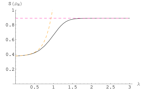
The canonical ensemble for gravity in asymptotically flat space at finite temperature is ill defined due to infrared instabilities, both perturbative (Jeans instability) and non-perturbative (nucleation of black holes). An infrared regulator is therefore necessary, the simplest one being the spherical box we employ here. Other regulators are possible; for example one can introduce a negative cosmological constant and work in asymptotically anti-de Sitter spaces. The thermodynamics of the system doesn’t depend qualitatively on which regulator is used. What is described in this subsection was largely the work of Gross, Perry, and Yaffe [1], Hawking and Page [25], and York [26], except for the calculations of the negative mode for the small black hole (resulting in figure 2) which are new.

We consider pure gravity in a rigid spherical box of radius $R$, which is kept in contact with a heat bath at a temperature $\beta^{-1}$. Note that it is the boundary that is kept at that temperature; even though the system is in thermal equilibrium, observers at different points inside the box may experience different temperatures due to gravitational red- and blue-shifting. According to the prescription of Euclidean Quantum Gravity, the partition function for this system is obtained by integrating $e^{-S[g]}$ over all Riemannian manifolds with boundary metric $S^{1}_{\beta}\times S^{2}_{R}$. This involves both summing over topologies and integrating over metrics.

The path integral is usually treated by the saddle point method. The number of saddle points (i.e. Ricci-flat metrics) depends on the dimensionless ratio $b\equiv\beta/(2\pi R)$. For any value of $b$, we have hot flat space, $S^{1}_{\beta}\times B^{3}_{R}$, where $B^{3}_{R}$ is a flat 3-ball of radius $R$. For $b<b_{\rm crit}=4/3\sqrt{3}\approx 0.77$ (in other words, at sufficiently high temperature), there are two other solutions. Both of them have topology $B^{2}\times S^{2}$, and both have the Euclidean Schwarzschild metric, but with different values of the horizon radius $r_{0}$:

$$ds^{2}=4r_{0}^{2}\left(1-\frac{r_{0}}{r}\right)d\tau^{2}+\left(1-\frac{r_{0}}{r}\right)^{-1}dr^{2}+r^{2}d\Omega_{2}^{2}.$$ (19)

The radial coordinate $r$ goes from $r_{0}$ (at the horizon) to $R$ (at the boundary). The imaginary time coordinate has periodicity $2\pi$, and the factor of $4r_{0}^{2}$ in the metric ensures smoothness at the horizon. For the circle to have the right length at the boundary, we must have

$$\beta=4\pi r_{0}\sqrt{1-\frac{r_{0}}{R}},$$ (20)

which fixes $r_{0}$ in terms of $\beta$ and $R$. For $b<b_{\rm crit}$ there are two solutions, with $r_{0}$ greater than and less than $\frac{2}{3}R$ respectively, which we refer to as the small and large black holes. Although it has not been proven, it is believed that these are the only saddle points for these boundary conditions [27], and this is what we will assume. In the limit that we remove the cutoff ($R\to\infty$, $\beta$ fixed), the small black hole goes over to the usual asymptotically flat Schwarzschild black hole ($r_{0}\to\beta/4\pi$), while the large black hole disappears ($r_{0}\to\infty$). Hot flat space persists as well in this limit, of course.

Figure 1: Action versus inverse temperature parameter $b\equiv\beta/(2\pi R)$ for the three saddle points. For $b>b_{\rm crit}$ only hot flat space is allowed, while for $b<b_{\rm crit}$ there are also small and large black hole solutions. At $b_{\rm HP}$ there is a first-order phase transition, the Hawking-Page transition: for $b>b_{\rm HP}$ flat space has the lowest action and therefore dominates thermodynamically, while for $b<b_{\rm HP}$ the large black hole dominates. The dashed lines indicate the three values of $b$ which will be used in later figures to display the qualitative behavior of the simulated Ricci flows. For this and all other figures we have chosen units such that $R=1$.

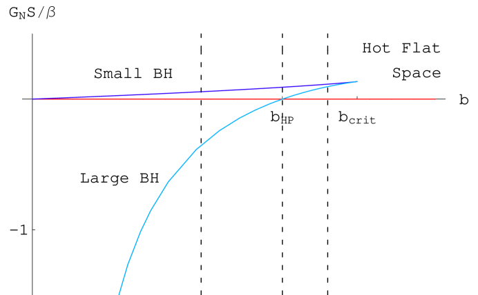
The system’s partition function, and therefore its thermodynamical properties, are dominated by the saddle point with the lowest value of the action (10). Choosing the constant $S_{0}$ to conform to the convention that flat space has zero action, the Schwarzschild solutions have action

$$S=\frac{\beta R}{G_{\rm N}}\left[1+\frac{4\pi r_{0}}{\beta}\left(\frac{3r_{0}}{4R}-1\right)\right].$$ (21)

The actions of the three saddle points are plotted as a function of $b$ in figure 1 (for this and all other figures we choose units such that $R=1$). We see that, for all temperatures where it exists, the small black hole has the largest action of all the saddle points. At low temperatures, specifically for $b>b_{\rm HP}=16/27\approx 0.59$, hot flat space dominates, while at higher temperatures the large black hole dominates. The first-order phase transition separating these two regimes is known as the Hawking-Page transition, by analogy with the same phenomenon in AdS [25].

Figure 2: Lowest eigenvalue $\mu$ of the Lichnerowicz operator $\Delta_{\rm L}$ on the black hole background (3.1). The small and large black holes are separated by the value $r_{0}/R=\frac{2}{3}$, where the eigenvalue passes from negative to positive. At this point the mode becomes tangent to this one-parameter family of solutions.

So far we have neglected the one-loop determinant in the saddle-point approximation to the path integral (not to mention the higher-loop corrections, which require an ultraviolet cutoff, such as string theory, to define). This correction is indeed negligible at small $\hbar$ (i.e. when the system is much larger than the Planck length), as long as all the eigenvalues are positive; otherwise the saddle point approximation doesn’t make sense. The operator in question, taking into account the rotation of the contours for the conformal modes, is

$${\Delta^{A}}_{C}=G^{AB}\frac{\partial^{2}S}{\partial g^{B}\partial g^{C}}.$$ (22)

Acting on a perturbation $h_{\mu\nu}$, ${\Delta^{A}}_{C}$ yields precisely (minus) the right-hand side of (8) (since the latter is just $\partial_{C}(-G^{AB}\partial_{B}S)h^{C}$, and of course $\partial_{B}S=0$ at the saddle point). This operator has infinitely many zero eigenvectors corresponding to pure gauge fluctuations, of the form $h^{\rm gauge}_{\mu\nu}=\nabla_{(\mu}w_{\nu)}$, which must be removed before the determinant is calculated. Since ${\Delta^{A}}_{C}$ is self-adjoint (with respect to $G_{AB}$) the physical eigenvectors are orthogonal to the pure gauge ones, and therefore correspond to fluctuations obeying the de Donder gauge condition $\nabla_{\mu}{h^{\mu}}_{\nu}-\frac{1}{2}\partial_{\nu}h=0$ (since $G_{AB}h_{\rm gauge}^{A}h^{B}=\int\sqrt{g}\nabla_{(\mu}w_{\nu)}(h^{\mu\nu}-\frac{1}{2}hg^{\mu\nu})=-\int\sqrt{g}w_{\nu}(\nabla_{\mu}h^{\mu\nu}-\frac{1}{2}\partial^{\nu}h)$). Restricting to the orthogonal complement of the gauge zero eigenvectors leaves these physical fluctuations on which ${\Delta^{A}}_{C}$ is just the Lichnerowicz operator $\Delta_{\rm L}$. (Equivalently, one can follow the Faddeev-Popov procedure and add a gauge-fixing term and ghosts [23].)

On the hot flat space background, $\Delta_{\rm L}$ is positive since the Riemann tensor vanishes and we have imposed Dirichlet boundary conditions. What about on the black hole backgrounds? In figure 2, the lowest eigenvalue of $\Delta_{\rm L}$ is plotted against $r_{0}$. For the large black hole ($r_{0}>\frac{2}{3}R$) it is positive, so like flat space it is indeed a good candidate for the thermal ground state of the system. In the regime where each has the lowest action, that action (divided by $\beta$) is the classical approximation to the system’s free energy. The small black hole, on the other hand, has a negative eigenvalue mode, the cavity generalization of the Gross-Perry-Yaffe instability of an asymptotically flat black hole [1]. As in the asymptotically flat case, this negative mode is mainly localized near the horizon, and preserves the $U(1)\times SO(3)$ isometries of the black hole (i.e. only depends on the radial coordinate). In past literature there is some confusion over the calculation of this mode in a cavity [29, 26, 4]. The important point is that, unlike in the asymptotically flat case, the mode is not traceless, since the cavity boundary conditions (constant Euclidean circle and 2-sphere radius) explicitly couple the trace and traceless modes. When this is taken into account one finds the curve in figure 2. (See Appendix A for details of the calculation.) In particular, as expected, one finds that the instability disappears exactly at the transition from the small to the large black hole, and therefore at the transition from local thermodynamic instability to stability. As pointed out by Hawking and Page [25], the zero mode that appears corresponds to slightly changing the black hole’s radius without altering the boundary condition.

What is the meaning of this negative mode? It has been argued to be related to the fact that the corresponding Lorentzian solution is locally thermodynamically unstable since it has a negative specific heat [2, 4, 5]. The negative mode also means that the Euclidean solution can serve as a bounce, representing thermal fluctuations that take hot flat space to the large black hole and vice versa, allowing the system to find its true ground state whichever side of the Hawking-Page transition it’s on [1, 26]. So although it is never the lowest-action saddle point, the small black hole nevertheless plays an important physical role in the system’s dynamics.

3.2 Kaluza-Klein interpretation

The three 4-dimensional Euclidean Ricci-flat geometries discussed in the previous subsection have an entirely different physical meaning if we interpret the circle direction, which was the imaginary time in the thermal context, instead as a Kaluza-Klein circle, and add a real time direction. The resulting 5-dimensional Lorentzian geometries are static solutions to the 5-dimensional Einstein equation with boundary $\mathbf{R}\times S^{1}_{\beta}\times S^{2}_{R}$. Note that, whereas in the 4-dimensional context these solutions are believed to be the only ones, in the 5-dimensional context there are certainly other static solutions, such as the uniform black string, which is (4-dimensional Lorentzian Schwarzschild)$\times S^{1}_{\beta}$. This is because there is an additional degree of freedom present, namely the time-time metric component.

What do these 5-dimensional solutions look like? First note that the ADM energy of each is equal to the Euclidean action of the corresponding 4-dimensional solution, plotted in figure 1. Furthermore, its linear stability is controlled by the 4-dimensional Lichnerowicz operator, since each mode of that operator can be put on shell by dressing it with a time dependence $e^{\pm i\sqrt{\mu}t}$, where $\mu$ is the $\Delta_{\rm L}$ eigenvalue. Let us fix $\beta$. For all values of $R$ we have “hot flat space”, which in this context is the Kaluza-Klein vacuum. As pointed out by Witten, although it is perturbatively stable, in the limit $R\to\infty$ the Kaluza-Klein vacuum is unstable due to nucleation of bubbles of nothing [30]. At large but finite $R$ we might therefore expect to find a ground state with negative energy; indeed we find the “large black hole”, which in this context is a static bubble of nothing that almost fills the container, but leaves a shell of “something” around the edge. This is also perturbatively stable. It seems likely that, for $b>b_{\rm HP}$, the true ground state is the Kaluza-Klein vacuum, while for $b<b_{\rm HP}$ it is the large bubble of nothing. Finally, we have the “small black hole”, or small bubble of nothing, which has higher energy than either the Kaluza-Klein vacuum or the large bubble, and is unstable.

In the context of string theory, such a gravitational instability is classified as a closed string tachyon. It is always interesting to study the world-sheet RG flow seeded by the vertex operator of such a tachyon, and to compare it to the system’s dynamical evolution. The classical evolution of the bubble perturbed by its unstable mode has in fact already been studied by Sarbach and Lehner using numerical simulation [7, 8]. Those simulations were performed without the box, which simplifies the analysis because it allows radiation to escape to infinity and the energy thereby to decrease. It was found that, when perturbed in one direction, the bubble grew without bound, while in the other it settled down to the black string. Apparently cosmic censorship prevents the system from classically reaching its local ground state, the Kaluza-Klein vacuum, because that would entail the appearance of a naked topology-changing singularity. (Of course quantum mechanically the black string would presumably evaporate, eventually settling down to the vacuum.) We will see in the next section that RG flow (which is well approximated by Ricci flow when the system is much larger than the string scale) does not suffer from such prudishness.

4 Where does the small black hole flow?

Let us call the negative mode of the small black hole $h_{\mu\nu}^{\rm GPY}$. If we perturb the small black hole by this mode and evolve the metric by Ricci flow, then, as long as it remains sufficiently small, the mode will grow exponentially. How does the metric evolve once it leaves the linear regime? At late times does it converge to one of the other saddle points? These are the questions we will answer in this section. Note that there are two different flows to follow, depending on whether $h_{\mu\nu}^{\rm GPY}$ is added with a positive or negative coefficient. These are physically distinct; in one direction the mode increases the horizon size and in the other decreases it. We will fix the convention that $h_{\mu\nu}^{\rm GPY}$ increases the horizon size. We performed numerical simulations of both of these Ricci flows at several values of the parameter $b$, below, at, and above the Hawking-Page value $b_{\rm HP}$. Details of the simulations are given in Appendix A. In this section we summarize the main results.

First, however, we would like to point out two obvious generalizations of our work. The first is to dimensions $D>4$. The second is to the small black hole in anti-de Sitter space, in which case the flow equation must be modified to include the cosmological constant term:

$$\frac{\partial g_{\mu\nu}}{\partial\lambda}=-2R_{\mu\nu}+2\Lambda g_{\mu\nu}.$$ (23)

In both cases the system is so closely analogous to the one we studied that it seems reasonable to guess that the behavior of the flows would be qualitatively the same.

We begin with the flow seeded by the perturbation $+h_{\mu\nu}^{\rm GPY}$. Since the perturbation does not break the black hole’s $U(1)\times SO(3)$ isometry group, the geometry enjoys this symmetry throughout the flow. In principle we would consider an infinitesimal perturbation. In practice for the initial data we perturbed the small black hole such that the horizon was increased in radius by one percent. This was sufficiently small that for some time the flow remained well described by the linear theory.

Figure 3: Euclidean time radius $T$ (red) and sphere radius $S$ (purple) against proper radial coordinate $\rho$, for the flow of the small black hole perturbed by $+h_{\mu\nu}^{\rm GPY}$, at $b=b_{\rm HP}\approx 0.59$. The boundary is at $\rho=0$. Snapshots are drawn at intervals of $\lambda$ of $0.05$. The heavy blue curves show those functions for the unperturbed small black hole. The heavy black curves show them for the corresponding large black hole, to which the flow clearly asymptotes at late times.

Figure 4: Horizon radius, $S(\rho_{\rm H})$, against $\lambda$ for small black hole perturbed by $+h_{\mu\nu}^{\rm GPY}$, at $b=0.40,0.59,0.70$ (the middle value equals $b_{\rm HP}$). The horizontal (red) dashed lines show the horizon radius for the corresponding large black hole, which the metric asymptotically converges to in each case. The curved (orange) dashed lines give the initial exponential growth of the negative mode.

To characterize the geometry it is sufficient to know the radii of the time circle and sphere, as functions of proper radial distance; in other words, to eliminate the gauge ambiguity the metric may be put into the form

$$ds^{2}=T(\rho)^{2}d\tau^{2}+d\rho^{2}+S(\rho)^{2}d\Omega_{2}^{2},$$ (24)

setting $\rho=0$ at the cavity wall (and $\rho<0$ in the cavity interior). $T(\rho)$ and $S(\rho)$ are plotted in figure 3 for a representative value of $b$, namely $b_{\rm HP}$. We see that the metric tends at large $\lambda$ to the large black hole solution. Let $\rho_{\rm H}$ to be the value of $\rho$ at the horizon. In figure 4 the horizon radius, i.e. $S(\rho_{\rm H})$, is plotted as a function of $\lambda$ for three different values of $b$. Again, in each case it asymptotes to the value for the large black hole. The initial growth of the small perturbation is governed by the linear theory, growing exponentially as $e^{-\mu\lambda}$, with $\mu$ given in figure 2. The same behavior was found for all values of $b$ tested: the metric relaxes to the large black hole solution.

4.1 Singularity and surgery

Figure 5: (Top) $T(\rho)$ (red) and $S(\rho)$ (purple) for the flow of the small black hole perturbed by $-h_{\mu\nu}^{\rm GPY}$, at $b=b_{\rm HP}$. Snapshots are drawn at intervals of $\lambda$ of $0.01$. The metric flows to a singularity, where the horizon shrinks to zero size. (Bottom) The metric after surgery, and the continuation of the Ricci flow. The metric asymptotically tends to flat space.

Figure 6: Horizon radius, $S(\rho_{H})$, as a function of $\lambda$ for the flow of the small black hole perturbed by $-h_{\mu\nu}^{\rm GPY}$. In all such flows the horizon collapses to zero size in finite time. The dashed lines show the initial exponential growth of the negative mode given by perturbation theory.

The behavior was quite different for the flows seeded by the perturbation $-h_{\mu\nu}^{\rm GPY}$. For every value of $b$ tested, after a finite flow time the horizon collapsed to a point, giving rise to a curvature singularity and stopping the flow. An example is shown in the top panel of figure 5. In figure 6, the horizon radius is plotted against $\lambda$ for the same three values of $b$ as shown in figure 4. More details of the local model for the singularity are given in appendix B.

Figure 7: An $S^{2}$ fibered over an interval will typically collapse under Ricci flow, producing a curvature singularity. This can be cured, allowing the flow to continue, by a local topology change known as a surgery.

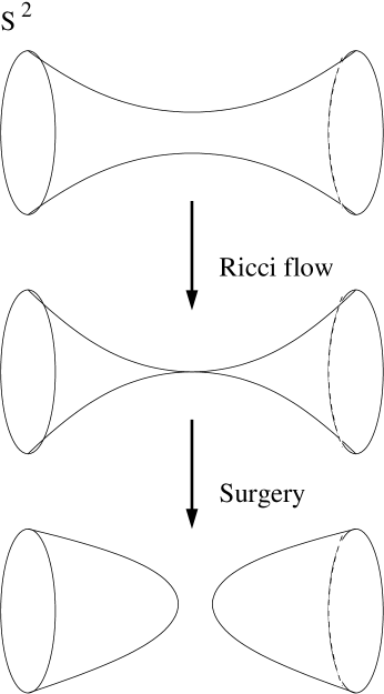
The spontaneous formation of singularities is generic in Ricci flow, and has been much studied by mathematicians, particularly in the case $D=3$. A common type of singularity that arises there, and is analogous to what we observe here, involves an $S^{2}$ fibered with varying radius over an interval (in a region of the manifold). The fibers’ positive curvature tends to make them shrink, and typically in finite time one of them will collapse to zero size, giving rise to a curvature singularity. In order to be able to continue the flow, mathematicians perform “surgery” on the singular manifold: a small neighborhood of the singular point is excised and replaced with a smooth metric. To avoid having the singularity re-appear, the topology is changed. Specifically, a piece of the base is removed, and smooth caps are sewn onto the two ends, as shown in figure 7. As a result of this process, the manifold (or at least this part of it) becomes disconnected, and the $S^{2}$ fibers, which were previously non-contractible, become contractible.

Figure 8: When perturbed by $-h_{\mu\nu}^{\rm GPY}$, the small black hole geometry (which is a 2-sphere fibered over a disk) evolves under Ricci flow until the horizon (the fiber over the center of the disk) collapses, giving rise to a singularity. The surgery we perform on the singular manifold involves excising a small disk from the base, making it an annulus, and making the sphere go to zero size on the inner boundary so that the resulting total space is smooth and topologically $S^{1}\times B^{3}$. We do this in such a way that the $U(1)\times SO(3)$ isometries of the geometry are preserved.

The singularity that appears in the Ricci flow of the black hole is quite analogous. Again, we have an $S^{2}$ fibered over a base, which in this case is a disk. And again, the fiber over a point on the base collapses to zero size after a finite flow time. We are therefore inspired by the above example to perform a similar surgery in order to continue the flow. Specifically, we excise a small disk from the base in a neighborhood of the singular fiber. The base thus becomes an annulus, and on its new inner boundary the fiber radius is made to go to zero in order to produce a smooth total space with topology $S^{1}\times B^{3}$; the $S^{2}$, which was non-contractible, is now contractible, and vice-versa for the $S^{1}$. The change to the metric is localized to a small distance $\epsilon$ from the singularity, and is required to respect the geometries $U(1)\times SO(3)$ isometry group. A cartoon of it is shown in figure 8. The resulting geometry can be seen in the example of figure 5 in the first snapshot of the bottom panel. Details of how the surgery was carried out are given in Appendix B.

Those who are interested in Ricci flow chiefly insofar as it approximates the RG flow of sigma models might ask the following question: What happens to the RG flow when the Ricci flow hits the singularity? When the curvatures become large in string units, the $\alpha^{\prime}$ corrections to the beta functions (16) become important, and Ricci flow is no longer a good approximation to RG flow. However, in general this will not be sufficient to stop a singularity from forming. This is shown by a simple example, namely the round metric on $S^{D}$ (otherwise known as the $O(N)$ model, with $N=D+1$). On the Ricci flow side, the sphere collapses to zero size in finite time. On the RG flow side, the model confines at a finite energy scale, and is massive below that scale. In the case of a sphere fibered over a base, it seems reasonable to guess that, similarly, when the fiber over some point on the base collapses (“confines”), it is removed from the target space, whose topology would change accordingly. In other words, we are proposing that, when the Ricci flow hits the singularity, the RG flow dynamically performs the surgery we have described above. The fact that this surgery is the unique local topology change that respects the manifold’s isometries means that the RG flow could hardly do otherwise.

After the surgery, the manifold has the same topology as hot flat space, and under Ricci flow the metric relaxes to that saddle point without encountering any further singularities. This can be seen in the bottom panel of figure 5; the same behavior was observed for the other values of $b$ tested. A key assumption is that, provided the metric deformation in the surgery is restricted to a region of size $\epsilon$, for small enough $\epsilon$ the details of the flow following the resolution will be independent of the precise nature of this deformation, and of the actual value of $\epsilon$. This is to be expected since the diffusive nature of Ricci flow quickly removes the fine details of the small resolved region. While we do not have a rigorous mathematical argument that this is the case, we found it to be true in our simulations, as shown in Appendix B. (The value of $\epsilon$ used to generate the singularity resolution in figure 5 was $0.07$).

5 A novel free energy diagram

Figure 9: Action $S$ versus flow time for the flows from the small black hole to hot flat space (left) and the large black hole (right), at $b=0.40,0.59,0.70$ (top, middle, bottom). The black lines indicate the topology $B^{2}\times S^{2}$, and the blue the topology $S^{1}\times B^{3}$, their join in the left plots being the point of singularity formation where the action remains continuous (up to a small numerical error in the case $b=0.40$).

Figure 10: $S/\beta$ against proper distance along the one-parameter family in the space of metrics defined by Ricci flow. In the left-hand (blue) part of each curve the topology is $S^{1}\times B^{3}$, while in the right-hand (black) part the topology is $B^{2}\times S^{2}$. As explained in the text, for these curves the value of $S/\beta$ can be interpreted as a free energy.

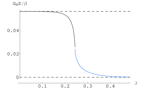
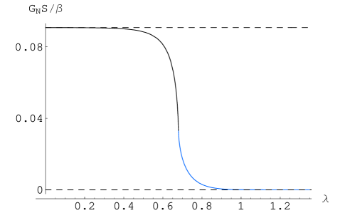
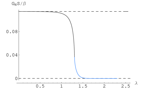
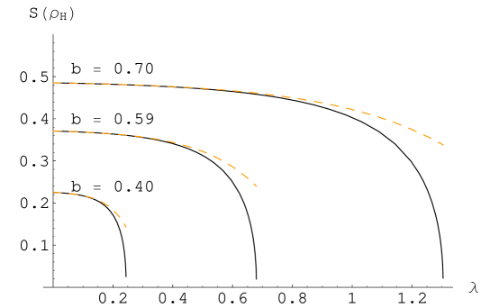
In the last section we saw that Ricci flow defines paths in the space of metrics connecting the small black hole to the large black hole and to hot flat space, in the latter case via a topology change. Since Ricci flow is gradient flow of the Einstein-Hilbert action (10), it is interesting to plot the action along the flow. This is done in figure 9 for the two flows at the three representative values of $b$ used in previous figures. We would like to point out two interesting features of these plots.

First, in the flow to hot flat space, the action stays finite when the singularity forms and is continuous across the topology change; although the Ricci scalar blows up on the horizon when it collapses, it remains integrable. The local singularity model described in Appendix B indicates that the divergence in the Ricci scalar is entirely due to the shrinking 2-sphere, so that $R\sim 1/S^{2}$ at the horizon. This is compensated by the factor of the 2-sphere volume in the measure $\sqrt{g}\sim TS^{2}$, and since $T\rightarrow 0$ at the horizon too, there is no contribution to the action from this singular point. From the point of view of the action, therefore, the singularity is harmless, and the surgery can be thought of as an infinitesimal change in the metric.

Second, the action is a monotonically decreasing function of $\lambda$. This is not a straightforward consequence of the fact that Ricci flow is gradient flow of the action, since the metric $G_{AB}$ is not positive definite (which is why we have used the term gradient flow, rather than gradient descent). The monotonicity of $S$ for these particular flows shows that they move through the space of metrics always in a spacelike direction; in other words, at every point along the flow we have

$$-\frac{\partial S}{\partial\lambda}=G_{AB}\frac{\partial g^{A}}{\partial\lambda}\frac{\partial g^{B}}{\partial\lambda}=\frac{1}{8\pi G_{\rm N}}\int_{M}\sqrt{g}\left(R_{\mu\nu}R^{\mu\nu}-\frac{1}{2}R^{2}\right)>0.$$ (25)

Hence the proper distance along the curves is well defined; it is given by

$$\alpha\equiv\int d\lambda\sqrt{G_{AB}\frac{\partial g^{A}}{\partial\lambda}\frac{\partial g^{B}}{\partial\lambda}}.$$ (26)

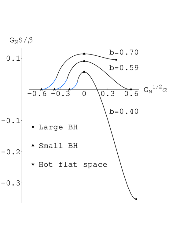
In figure 10, we plot $S$ against $\alpha$, putting the two flows starting at the small black hole back to back where they join smoothly. Note that the saddle points are a finite distance away from each other along these curves.

Figure 10 bears a strong resemblance to a free energy diagram. Can it be interpreted as such in a physically meaningful way? To clarify this question, let us first briefly review how free energy diagrams are conventionally defined. Suppose one is interested in knowing the expectation value of some macroscopic observable $a$ (for example, the magnetization of a ferromagnet). To do this, one calculates the free energy $f(a)$ in the sub-ensemble where the value of $a$ is fixed; this calculation can, for example, be done in a saddle point approximation. The expectation value of $a$, and the actual free energy $F$ of the system, are determined by integrating $e^{-\beta f(a)}$ over $a$, which, again in a saddle point approximation, amounts to minimizing $f(a)$. In other words, in calculating the partition function the degrees of freedom are integrated over in two steps: first everything but $a$, then $a$ itself. The free energy diagram appears between these steps.

Let us illustrate these ideas for the case at hand, gravity in a cavity; our discussion follows York [26]. We choose as our macroscopic observable $a$ the horizon area. Working on the topology $B^{2}\times S^{2}$, the horizon area is fixed by adding a Lagrange multiplier term to the action:

$$S_{a}[g]=S[g]+\lambda\left(A[g]-a\right).$$ (27)

This term introduces into the Einstein equation a source term in the form of a two-dimensional delta function on the disk at the location of the horizon, leading to a conical singularity. The saddle point of the new action is therefore the Euclidean Schwarzschild metric (19), but with $r_{0}$ determined by $4\pi r_{0}^{2}=a$ rather than by (20), and with the periodicity of $\tau$ equal to $\beta/(2r_{0}\sqrt{1-r_{0}/R})$ rather than $2\pi$. The action of this solution is easily calculated, giving a free energy of the familiar form “energy minus temperature times entropy”:

$$f=\frac{S}{\beta}=\frac{R}{G_{\rm N}}\left[1-\sqrt{1-\sqrt{\frac{a}{4\pi R^{2}}}}-\frac{a}{4\beta R}\right].$$ (28)

Following Whiting and York [2], we plot $f$ in figure LABEL:fig:York, where the three saddle points are easily identified. Hot flat space is at $a=0$; in fact the topology change from $B^{2}\times S^{2}$ to $S^{1}\times B^{3}$ occurs at that very point on the free energy diagram (which to some extent excuses the rather singular behavior of $f$ there).

Let us now return to our putative free energy plot, figure 10, derived from the Ricci flows. $S/\beta$, which is plotted for each point $g^{A}(\lambda)$ along the flow, can justifiably be called a free energy if it is the saddle point approximation to the partition function of some sub-ensemble. We will now show that it is. First note that the gradient of $S$, restricted to the directions orthogonal to the curve $g^{A}(\lambda)$, vanishes, since the tangent vector to the curve is in the gradient direction. Furthermore the second-derivative operator ${\Delta^{A}}_{C}$ (defined in (22)) restricted to those directions is positive, since its only negative direction is along the curve. Therefore the saddle point approximation to the path integral along the directions orthogonal to the curve is given by the value of the action on the curve. This defines the sub-ensembles for which figure 10 is the appropriate free energy diagram. It is obviously crucial for this construction that $g^{A}(\lambda)$ is defined by a gradient flow of the action. In fact the same construction could be applied to any system equipped with a natural metric on the configuration space. The major difference between this construction and the conventional one is that this one does not require singling out a particular macroscopic observable.

We note that York’s prescription of fixing the horizon area is motivated by the Lorentzian dynamics of an evaporating black hole, since the horizon size is the slow variable in that process. From the point of view of the canonical Euclidean path integral, York’s construction is less natural, as seen by the conical singularity that arises in the Euclidean geometries.

We conclude by commenting that in the context of the AdS-CFT duality it is interesting to consider the constrained free energy of asymptotically AdS spacetimes with and without horizons. On the field theory side of the correspondence, at weak coupling, one can naturally compute such an off-shell free energy [33], which has a similar appearance to ours. At strong coupling, this is expected to be similar, with the extrema corresponding on the gravity side to exactly the small and large AdS-Schwarzschild black holes, and thermal AdS, and the Hawking-Page phase transition being interpreted in field theory as the confinement/deconfinement transition. We note however, that the constraint in the field theory is placed on the expectation value of the trace of the Polyakov loop. On the gravity side, this presumably translates into a constraint on the area of a string world sheet wrapping the thermal Euclidean time circle at the asymptotic AdS boundary. Hence this is a different constraint than the one imposed by York; it would be interesting to find the relevant constrained off-shell geometries.

Appendix A Details of Ricci flow simulation

In practice we choose units so that $R=1$. Then the small black holes are given by (19) for $r_{0}<\frac{2}{3}$, and the large black holes with $\frac{2}{3}<r_{0}<1$. Our boundary conditions on the box wall are fixing the sphere radius ($R=1$), and fixing the Euclidean time period $\beta=2\pi b$. We start with the small black hole metric, perturbed by a suitably small $h^{\mathrm{GPY}}$ which satisfies the above boundary conditions. For the data presented here, the amplitude of the perturbation was chosen to change the horizon radius by one percent. The initial perturbation $\pm h^{\mathrm{GPY}}$ respects the $U(1)\times SO(3)$ isometry of the black hole, and hence the entire flow will share this isometry. We exploit this, using the metric,

$$ds^{2}=e^{2A}r^{2}b^{2}d\tau^{2}+e^{2B}dr^{2}+e^{2C}d\Omega_{2}^{2}$$ (29)

where $\tau$ has period $2\pi$. Since we initially are interested in the topology $B^{2}\times S^{2}$ then $A,B,C$ are finite functions of $r$ and the flow parameter $\lambda$, and we take $0\leq r\leq 1$. At $r=1$ we take $A=0,C=0$ appropriate to our finite box boundary condition. The new ‘boundary’ at $r=0$ is fictitious, since we know the Euclidean black hole geometries are smooth manifolds without an interior boundary. Regularity of the Ricci flow equations implies $A_{,r}=B_{,r}=C_{,r}=0$ at this origin. In particular, one finds as expected that $(A/C)|_{r=0}$ is preserved under the flow, and hence an initially smooth 4-d solution remains smooth, without developing conical singularities.

For asymptotically flat spacetime we are free to make any choice of $\xi_{\mu}$ in (3). However, on a manifold with boundary we must take care. We have covered our manifold with coordinates such that the boundary is at $r=1$. Hence Ricci flow with $\xi_{\mu}=0$ is only equivalent to flow with non-vanishing $\xi_{\mu}$ provided $\xi_{r}=0$ at $r=1$. Otherwise the coordinate location of the boundary will change during the flow.

Subject to $\xi_{r}=0$ at the box wall, we are free to specify any $\xi_{\mu}$ in (3). We make the choice,

$$\xi^{\mu}=-\Delta_{\rm S}x^{\mu}+\Delta_{\rm S}x^{\mu}|_{A,B,C=0}$$ (30)

where $x^{\mu}$ are the coordinates and $\Delta_{\rm S}$ is the scalar Laplacian. This choice is similar to the DeTurck flow, and ensures strong parabolicity—in analogy with the harmonic coordinate choice which yields strongly elliptic Euclidean Einstein equations. The flow equation becomes,

$$\frac{d}{d\lambda}g_{\mu\nu}=\Delta_{\rm S}g_{\mu\nu}+F(g,\nabla g)$$ (31)

where on the right-hand side we have only explicitly displayed the second derivative terms, which are simply given by the scalar Laplacian. This parabolic flow requires boundary conditions for all components of the metric, namely $A,B,C$, at the cavity wall. There we take $A=0$, $C=0$, since we fix the induced metric there. The only non-zero component of $\xi_{\mu}$ is,

$$\xi_{r}=-\partial_{r}A+\partial_{r}B-2\partial_{r}C$$ (32)

and hence we see the boundary condition that $\xi_{r}=0$ at $r=1$ translates into a boundary condition of the gradient of $B$. Hence $A,B,C$ all have boundary conditions on their value, or gradient, compatible with the parabolic flow.

It is interesting to note that the 4-d Schwarzschild metric takes the elegant analytic form,

$$ds^{2}=r_{0}^{2}\left[4(1-r_{0})\left(r^{2}d\tau^{2}+\frac{1}{(1-(1-r_{0})r^{2})^{4}}dr^{2}\right)+\frac{1}{(1-(1-r_{0})r^{2})^{2}}d\Omega_{2}^{2}\right]$$ (33)

in the coordinate system where $\xi^{\mu}=0$ everywhere, and furthermore the derived metric functions $A,B,C$ are finite as we require. Hence we take this as a background metric. We compute $\pm h^{\mathrm{GPY}}$ using the Lichnerowicz operator in this background, also in the gauge $\xi^{\mu}=0$. As usual, the resulting coupled ordinary differential equations are best solved as a shooting problem. Note that the condition $\xi_{r}=0$ together with $A=C=0$ implies that we cannot expect $B=0$ at the cavity wall. As mentioned in the main text, this means the mode cannot be traceless there, which clearly would also require $B=0$. Hence the cavity wall couples the trace and traceless perturbations, unlike in the asymptotically flat or AdS computations.

Having computed this, we use it to perturb the small black hole with the amplitude chosen as described above. This forms our initial data for the Ricci flow, and ensures our condition $\xi_{r}=0$ is satisfied at the box wall.

We simulated the full Ricci flows for

$$b=0.10,0.20,0.30,0.40,0.59,0.62,0.64,0.66,0.68,0.70,0.72,0.74.$$ (34)

The value $b=16/27\approx 0.59$ gives the middle dotted line in figure 1 where the free energies of hot flat space and the large black hole are equal. The values $0.40$ and $0.70$ give the other dotted lines in this figure. Properties of the flows for these three values are displayed in the various figures here, but we obtained qualitatively similar behavior for all values of $b$ above.

We used a uniform lattice discretization, and solve the Ricci flow using the implicit Crank-Nicholson method since it has diffusive character. We performed flows at various resolutions and confirmed the correct convergence to the continuum. Data presented here use $dr=0.0025$, i.e. 400 points.

After singularity resolution for the $-h^{\mathrm{GPY}}$ flows, we are interested in the topology $S^{1}\times B^{3}$ where we use the metric,

$$ds^{2}=e^{2\tilde{A}}b^{2}d\tau^{2}+e^{2\tilde{B}}dr^{2}+e^{2\tilde{C}}r^{2}d\Omega^{2}$$ (35)

and take finite $\tilde{A},\tilde{B},\tilde{C}$, again with $0\leq r\leq 1$. Now regularity of the Ricci flow equations at $r=0$ requires the boundary conditions $\tilde{B}=\tilde{C}$ and $\tilde{A}_{,r}=\tilde{B}_{,r}=\tilde{C}_{,r}=0$ at the origin, ensuring again a regular 4-d Euclidean geometry. As for (29) we make the choice,

$$\xi^{\mu}=-\Delta_{\rm S}x^{\mu}+\Delta_{\rm S}x^{\mu}|_{\tilde{A},\tilde{B},\tilde{C}=0},$$ (36)

again ensuring a strongly parabolic flow. As above, we require $A=C=0$ at the cavity wall, and obtain a boundary condition for $B$ from the condition that $\xi_{r}$ vanishes there.

Appendix B More on the singularity and surgery

Figure 12: $(R_{\alpha\beta\mu\nu}R^{\alpha\beta\mu\nu})^{1/4}$ against $r$, at different values of flow time as the singularity is approached, for the flow seeded by $-h_{\mu\nu}^{\rm GPY}$ with $b=0.59$.

Figure 13: $T(\rho)$ and $S(\rho)$ plotted against proper distance from the horizon, $(\rho-\rho_{H})$, in the vicinity of the horizon as the singularity is approached. Snapshots are taken at intervals of $\lambda$ of $0.002$.

In figure 12 we plot the curvature invariant $(R_{\alpha\beta\mu\nu}R^{\alpha\beta\mu\nu})^{1/4}$ for the flow generated by $-h^{\rm{GPY}}_{\mu\nu}$. We see that, as expected, the shrinking of the 2-sphere at the horizon leads to an increasingly singular curvature there. This nature of the singularity that forms may be seen by plotting $T,S$ in the vicinity of the horizon, as in figure 13. We see that since the geometry is smooth before the singular flow time, the gradient of $T$ is fixed at the horizon. The interesting part of the geometry is then the shrinking 2-sphere, and we see that whilst the size of this at the horizon decreases towards the singularity, the rate of expansion of the sphere away from the horizon appears to remain zero as the singularity is approached. Hence the local model for this singularity is simply $\mathbf{R}^{2}\times S^{2}$. Note that the only other option we know of for the singularity model would have been a cone with base $S^{1}\times S^{2}$.

Figure 14: Comparison of two different resolutions of the singularity formed in the $b=0.59$ flow. The size of the region where the surgery is performed is different in the two cases, and characterized by $\epsilon=0.07$ (orange) and $0.14$ (blue), but the resulting flows appear very similar after a short time. The geometries are plotted for intervals $0.002$ in $\lambda$ after the resolution. Both flows eventually tend to flat space, although this is not shown here for clarity.

We wish to perform surgery on the geometry just before the singularity is reached. We do this by taking the geometry at some flow time $\lambda_{0}$ before the singularity, with functions $A,B,C$ in 29, and moving to the topology 35, with,

$$e^{2\tilde{A}} = (\epsilon^{2}+r^{2})e^{2A}$$ (37)

$$e^{2\tilde{B}} = e^{2B}$$ (38)

$$e^{2\tilde{C}} = \frac{1}{(\epsilon^{2}+r^{2})}e^{2C}$$ (39)

with,

$$\epsilon=e^{C-B}|_{r=0}.$$ (40)

Note the resulting geometry with topology $S^{1}\times B^{3}$ is smooth, and for $r\gg\epsilon$ the geometry before and after surgery is the same, the modification only occurring for $r\sim\epsilon$. The size of $\epsilon$ therefore determines the size of the region where surgery is performed. This is smaller the closer one takes $\lambda_{0}$ to the singularity. In figure 14 we show two flows for $b=0.59$ which use different values of $\lambda_{0}$, giving $\epsilon=0.07$ and $0.14$. We note that both do indeed flow to flat space, and furthermore, the large scale form of the flow appears to be insensitive to the details of the resolution.

References

- [1] D. J. Gross, M. J. Perry, and L. G. Yaffe, Instability of flat space at finite temperature, Phys. Rev. D25 (1982) 330–355.
- [2] B. F. Whiting and J.W. York, Jr., Action principle and partition function for the gravitational field in black hole topologies, Phys. Rev. Lett. 61 (1988) 1336.
- [3] B. F. Whiting, Black holes and thermodynamics, Class. Quant. Grav. 7 (1990) 15–18.
- [4] T. Prestidge, Dynamic and thermodynamic stability and negative modes in Schwarzschild-anti-de Sitter, Phys. Rev. D61 (2000) 084002, [hep-th/9907163].
- [5] H. S. Reall, Classical and thermodynamic stability of black branes, Phys. Rev. D64 (2001) 044005, [hep-th/0104071].
- [6] M. Gutperle, M. Headrick, S. Minwalla, and V. Schomerus, Space-time energy decreases under world-sheet RG flow, JHEP 01 (2003) 073, [hep-th/0211063].
- [7] O. Sarbach and L. Lehner, No naked singularities in homogeneous, spherically symmetric bubble spacetimes?, Phys. Rev. D69 (2004) 021901, [hep-th/0308116].
- [8] O. Sarbach and L. Lehner, Critical bubbles and implications for critical black strings, Phys. Rev. D71 (2005) 026002, [hep-th/0407265].
- [9] K. Hori and A. Kapustin, Duality of the fermionic 2d black hole and N = 2 Liouville theory as mirror symmetry, JHEP 08 (2001) 045, [hep-th/0104202].
- [10] D. Garfinkle and J. Isenberg, Critical behavior in Ricci flow, math.dg/0306129.
- [11] D. Garfinkle and J. Isenberg, Numerical studies of the behavior of Ricci flow, in Geometric evolution equations, vol. 367 of Contemp. Math., pp. 103–114. Amer. Math. Soc., Providence, RI, 2005.
- [12] M. Headrick and T. Wiseman, Numerical Ricci-flat metrics on K3, Class. Quant. Grav. 22 (2005) 4931–4960, [hep-th/0506129].
- [13] D. H. Friedan, Nonlinear models in two + epsilon dimensions, Ann. Phys. 163 (1985) 318.
- [14] R. S. Hamilton, Three-manifolds with positive Ricci curvature, J. Differential Geom. 17 (1982), no. 2 255–306.
- [15] G. Perelman, The entropy formula for the Ricci flow and its geometric applications, math.DG/0211159.
- [16] G. Perelman, Ricci flow with surgery on three-manifolds, math.DG/0303109.
- [17] J. W. Morgan, Recent progress on the Poincaré conjecture and the classification of 3-manifolds, Bull. Amer. Math. Soc. (N.S.) 42 (2005), no. 1 57–78 (electronic).
- [18] P. Topping, Lectures on the Ricci flow, http://www.maths.warwick.ac.uk/~topping/RFnotes.html.
- [19] B. Chow and D. Knopf, The Ricci flow: an introduction, vol. 110 of Mathematical Surveys and Monographs. American Mathematical Society, Providence, RI, 2004.
- [20] D. M. DeTurck, Deforming metrics in the direction of their Ricci tensors, J. Differential Geom. 18 (1983), no. 1 157–162.
- [21] Y. Shen, On Ricci deformation of a Riemannian metric on manifold with boundary, Pacific J. Math. 173 (1996), no. 1 203–221.
- [22] B. S. DeWitt, Quantum theory of gravity. 1. the canonical theory, Phys. Rev. 160 (1967) 1113–1148.
- [23] G. W. Gibbons, S. W. Hawking, and M. J. Perry, Path integrals and the indefiniteness of the gravitational action, Nucl. Phys. B138 (1978) 141.
- [24] D. Z. Freedman, M. Headrick, and A. Lawrence, On closed string tachyon dynamics, Phys. Rev. D73 (2006) 066015, [hep-th/0510126].
- [25] S. W. Hawking and D. N. Page, Thermodynamics of black holes in anti-de Sitter space, Commun. Math. Phys. 87 (1983) 577.
- [26] J.W. York, Jr., Black hole thermodynamics and the Euclidean Einstein action, Phys. Rev. D33 (1986) 2092–2099.
- [27] G. Gibbons. Private communication.
- [28] J. J. Atick and E. Witten, The Hagedorn transition and the number of degrees of freedom of string theory, Nucl. Phys. B310 (1988) 291–334.
- [29] B. Allen, Euclidean Schwarzschild negative mode, Phys. Rev. D30 (1984) 1153–1157.
- [30] E. Witten, Instability of the Kaluza-Klein vacuum, Nucl. Phys. B195 (1982) 481.
- [31] K. Copsey and G. T. Horowitz, Gravity dual of gauge theory on , hep-th/0602003.
- [32] A. Adams, X. Liu, J. McGreevy, A. Saltman, and E. Silverstein, Things fall apart: Topology change from winding tachyons, JHEP 10 (2005) 033, [hep-th/0502021].
- [33] O. Aharony, J. Marsano, S. Minwalla, K. Papadodimas, and M. Van Raamsdonk, The Hagedorn / deconfinement phase transition in weakly coupled large N gauge theories, Adv. Theor. Math. Phys. 8 (2004) 603–696, [hep-th/0310285].
- [34] J. L. F. Barbon and E. Rabinovici, Closed-string tachyons and the Hagedorn transition in AdS space, JHEP 03 (2002) 057, [hep-th/0112173].
- [35] J. L. F. Barbon and E. Rabinovici, Remarks on black hole instabilities and closed string tachyons, Found. Phys. 33 (2003) 145–165, [hep-th/0211212].
- [36] J. L. F. Barbon and E. Rabinovici, Touring the Hagedorn ridge, hep-th/0407236.
- [37] Y. S. Myung, Tachyon condensation and off-shell gravity / gauge duality, hep-th/0604057.