Soliton Junctions
in the Large Magnetic Flux Limit

Stefano Bolognesi and Sven Bjarke Gudnason

The Niels Bohr Institute, Blegdamsvej 17, DK-2100 Copenhagen Ø, Denmark

Abstract

We study the flux tube junctions in the limit of large magnetic flux. In this limit the flux tube becomes a wall vortex which is a wall of negligible thickness (compared to the radius of the tube) compactified on a cylinder and stabilized by the flux inside. This wall surface can also assume different shapes that correspond to soliton junctions. We can have a flux tube that ends on a wall, a flux tube that ends on a monopole and more generic configurations containing all three of them. In this paper we find the differential equations that describe the shape of the wall vortex surface for these junctions. We will restrict to the cases of cylindrical symmetry. We also solve numerically these differential equations for various kinds of junctions. We finally find an interesting relation between soliton junctions and dynamical systems.

June, 2006

1 Introduction

In a recent series of works [1, 2, 3] we studied the behavior of the Abrikosov-Nielsen-Olesen (ANO) vortex [4] in the large $n$ limit, where $n$ is the number of quanta of magnetic flux carried by the vortex. We have seen that in this limit the ANO vortex becomes essentially a bag, analogous to the bag models of hadrons [6, 5]. We now briefly review the essential results.

The theory under consideration is the Abelian-Higgs model

$$\mathcal{L}=-\frac{1}{4}F_{\mu\nu}F^{\mu\nu}-|(\partial_{\mu}-ieA_{\mu})q|^{2}-V(|q|)\ ,$$ (1.1)

where the potential is chosen such that it has a minimum in the Higgs phase $|q|=q_{0}\neq 0$. The ANO vortex is a string-like soliton that extends in time and one spatial dimension. The simplest way to describe it is to introduce cylindrical coordinates $(z,r,\theta)$ and orientate it in the $\hat{z}$ direction. The fields can then be put into the following form

$$q =q_{0}e^{in\theta}\,q(r)\ ,$$ (1.2)

$$A_{\theta} =\frac{n}{er}\,A(r)\ .$$

The problem is now to evaluate the profile functions $q(r)$ and $A(r)$ subjected to the boundary conditions $q(0)=0$, $q(\infty)=q_{0}$ and $A(0)=0$, $A(\infty)=1$. The claim is that, for every Higgs-like potential $V$, in the large $n$ limit the profiles become

$$\lim_{n\rightarrow\infty}q(r) \rightarrow\theta_{H}(r-R_{\mathrm{V}})\ ,$$ (1.3)

$$\lim_{n\rightarrow\infty}A(r) \rightarrow\left\{\begin{array}[c]{cc}r^{2}/{R_{\mathrm{V}}}^{2}&0\leq r\leq R_{\mathrm{V}}\ ,\\ 1&r>R_{\mathrm{V}}\ .\end{array}\right.$$ (1.6)

This conjecture has been proved in [3] by numerical computations. We show in Figure 1 the result obtained for the BPS potential and $n=25,000$.

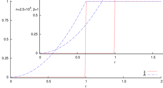
Figure 1: This plot is one of the outcomes of the numerical analysis made in [3]. It shows the profile functions $q(r)$ (red/solid line) and $A(r)$ (blue/dashed line) for the BPS potential ($\beta=1$) and winding number $n=25,000$.

The step function of the profile $q(r)$ reveals the presence of a substructure: a domain wall interpolating between the Coulomb phase $q=0$ and the Higgs phase $q=q_{0}$. For this reason we have named this object wall vortex.

The wall vortex is essentially a bag, such as the ones used in the context of the bag models of hadrons. A domain wall of thickness $\Delta_{\mathrm{W}}$ and tension $T_{\mathrm{W}}$ is wrapped onto a cylinder of radius $R$. The bag model is a good approximation when the thickness of the wall is small compared to the radius of the vortex. There are three energy terms that must be considered. The first one comes from the tension of the wall and is proportional to the radius $R$. The second comes from the energy density of the interior of the bag and is proportional to $R^{2}$. The third energy term comes from the magnetic flux and is proportional to $1/R^{2}$. When they are summed we obtain the tension as function of the radius $R$:

$$T(R)=\frac{2\pi n^{2}}{e^{2}R^{2}}+T_{\mathrm{W}}2\pi R+\varepsilon_{0}\pi R^{2}\ .$$ (1.7)

The radius of the vortex $R_{\mathrm{V}}$ is the one that minimizes this expression. Physically we can understand it in this way. When we derive (1.7) with respect to $R$ we obtain the various forces that act on the surface of the bag. The first two terms bring a collapse force that tends to squeeze the tube. The third term acts instead as a pressure that tends to expand the tube. When the two opposite forces are equilibrated we have a stable configuration.

The aim of the present paper is to study a more generic embedding of the wall vortex in the three dimensional space. The configuration (1.7) has the maximal number of possible symmetries, it is invariant under cylindrical rotation and $z$ translation. Now we want to relax the last condition, namely we consider a wall that has only cylindrical symmetry. The radius $R$ is no longer a constant but a function $R=f(z)$, and the force balance will not be an algebraic equation but a system of differential equations.

Solitons in the Higgs phase have received great attention in the last years. A lot of different models in different limits have been investigated and the jungle of solitons and soliton junctions is enormously vast. Here we just mention the works that have mostly influenced the present paper: solitons in nonlinear sigma models [15, 16], vortices and walls in supersymmetric models with a Fayet-Ilioupoulos term [7, 8, 9], the moduli matrix approach [17, 18, 19], nonabelian vortices and their junction with nonabelian monopoles [10, 11, 12], the vortex-monopole-vortex junction [13, 14] and also the MQCD realization of soliton junctions [23, 24, 25]. We find particularly amazing the various relations between the two fundamental solitons in the Higgs phase: the vortex and the wall. More recent works are [20, 21, 22]. The large magnetic flux limit is a very general approach, it applies to the Abelian-Higgs model (1.1) that is the basic building block of all the more sophisticated theories that contain solitons in the Higgs phase. Our result can thus be applied also to these theories and maybe explain some of the various relations between walls and vortices. Some of these recent developments on solitons are summarized in the reviews [26, 27].

The paper is divided into two main parts. In Section 2 we derive the system of differential equations that governs the vortex junctions. In Section 3 we explicitly study the physical solutions of the differential equations. We conclude in 4 with comments and possible applications.

2 The Differential Equations

To obtain the differential equations for the profile $r=f(z)$ we proceed in three steps. First in Subsection 2.1 we redo the wall vortex analysis interpreting the minimization of $T(R)$ (1.7) as a balance of forces acting on the wall. Then in Subsection 2.2 we find the mechanical forces (the ones coming from the tension $T_{\mathrm{W}}$ and the energy density $\varepsilon_{0}$) for a generic profile with cylindrical symmetry. Finally in Subsection 2.3 we obtain the master equation governing the profile $f(z)$.

2.1 Wall vortex redone

The wall vortex radius is obtained by the minimization of the function $T(R).$ The derivative of (1.7) divided by the perimeter $2\pi R$ gives

$$-\frac{2n^{2}}{e^{2}R^{4}}+\frac{T_{\mathrm{W}}}{R}+\varepsilon_{0}=0\ .$$ (2.1)

This equation can be interpreted as a balance of forces per unit of area acting on the surface of the wall. Preceding from the right to left of (2.1) we have:

• The energy density $\varepsilon_{0}$ is a force per unit area directed inwards;

• The tension of the wall $T_{\mathrm{W}}$ divided by the radius of curvature $R$ is a force per unit area directed inwards. Note that the other radius of curvature of the surface is infinite and does not contribute any extra force;

• The remaining term $-\frac{2n^{2}}{e^{2}R^{4}}$ must be interpreted as a force due to the magnetic field on the boundary of the cylinder and directed outwards. To check the consistency, note that since the flux carried by the wall vortex is $\Phi_{B}=\frac{2\pi n}{e}$ and the magnetic field is $B=\frac{2n}{eR^{2}}$, the term $\frac{2n^{2}}{e^{2}R^{4}}$ is exactly equal to the magnetic field energy density $\frac{B^{2}}{2}$.

There is a simple way to understand the origin of the magnetic field force $\frac{B^{2}}{2}$.

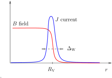
Figure 2: The magnetic field $B$ and the magnetic current $J$ at the boundary of the wall vortex.

We can write the magnetic field as a function of the radius $B(r)$ where $B=\frac{2n}{eR^{2}}$ inside the wall vortex, $B=0$ outside and the transition is encoded in the function $B(r)$. Using the Maxwell equation $\vec{\nabla}\wedge\vec{B}\ =\vec{J}\$ we find $J(r)=\frac{dB(r)}{dr}$. The force per unit volume acting on density current is $\vec{F}=\vec{J}\wedge\vec{B}$ thus the force per unit of area acting on the surface of the wall is

$$\int B(r)\frac{dB(r)}{dr}dr=\int d\left(\frac{B\left(r\right)^{2}}{2}\right)=\left.\frac{B^{2}}{2}\right|_{\mathrm{inside}}\ ,$$ (2.2)

and is directed outwards. Note that this force is independent on the precise behavior of the function $B(r)$.

2.2 Mechanical Forces

Now we want to find the mechanical forces in the case of a generic profile $r=f(z)$. We proceed in this way. First we write the mechanical energy as an integral with respect to $z$ of the surface element times the tension $T_{\mathrm{W}}$ plus the volume element times the energy density $\varepsilon_{0}$:

$$E_{\mathrm{mech}}=\int dz\left(2\,\pi T_{\mathrm{W}}\,f\,\sqrt{1+f^{\prime\,2}}\,+\pi\varepsilon_{0~{}}f^{2}\right)~{}.$$ (2.3)

In absence of the magnetic field, the profile $f(z)$ is the solution to the Euler-Lagrange equations obtained by varying $E_{\mathrm{mech}}$:

$$2\pi T_{\mathrm{W}}~{}\frac{1+f^{\prime\,2}-f^{\prime\prime}\,f}{(1+{f^{\prime}}^{2})^{3/2}}+2\pi\varepsilon_{0}~{}f\ =0~{}.$$ (2.4)

Dividing by the perimeter $2\pi f$ one obtains the forces per unit area

$$T_{\mathrm{W}}\frac{1}{f(1+f^{\prime\,2})^{1/2}}-T_{\mathrm{W}}\frac{~{}f^{\prime\prime}}{(1+{f^{\prime}}^{2})^{3/2}}+\varepsilon_{0}=0$$ (2.5)

$\varepsilon_{0}$ is a force per unit area due to the internal energy density and it does not depend on the profile. The other two terms can be identified with the tension divided by the two radia of curvature of the surface. To verify it we now compute the two radia of curvature geometrically.

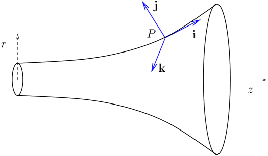
Figure 3: Geometry of the wall vortex surface.

Take a point $P=(r,\phi,z)=(f(z),0,z)$, or in the Cartesian coordinates, $(x,y,z)=(f(z),0,z)$ on the surface. The tangent vector in that point is

$$\mathbf{i}=(\frac{f^{\prime}}{\sqrt{1+f^{\prime\,2}}},0,\frac{1}{\sqrt{1+f^{\prime\,2}}})~{}.$$ (2.6)

The plane orthogonal to $\mathbf{i}$ and passing through $P$ is

$$f^{\prime}\,(X-f)+(Z-z)=0~{}.$$ (2.7)

The unit orthonormal vectors lying on the plane (2.7) and orthogonal to $\mathbf{i}$ are $(\mathbf{j},\,\mathbf{k})$, where

$$\mathbf{j}=(\frac{-1}{\sqrt{1+f^{\prime\,2}}},0,\frac{f^{\prime}}{\sqrt{1+f^{\prime\,2}}})~{},\qquad\mathbf{k}=\mathbf{i}\wedge\mathbf{j}=(0,1,0)~{}.$$ (2.8)

One radius of curvature is in the plane $(\mathbf{i},\,\mathbf{j})$ and is the easiest one to compute

$$\frac{1}{R_{1}}=-\frac{f^{\prime\prime}}{(1+f^{\prime 2})^{2/3}}~{}.$$ (2.9)

It is directed outwards in case of positive $f^{\prime\prime}$ or inwards in case of negative $f^{\prime\prime}$. The other radius of curvature is in the plane $(\mathbf{j},\,\mathbf{k})$ defined by Eq. (2.7). The curvature inwards that lies in the plane $(\mathbf{j},\,\mathbf{k})$ is

$$\frac{1}{R_{2}}=\frac{1}{f\,\sqrt{1+f^{\prime 2}}}~{}.$$ (2.10)

In summary, the force inwards and outwards at the point $P=(f(z),z)$ is respectively

$$F_{1}=\frac{1}{f\,\sqrt{1+f^{\prime 2}}}\,T_{\mathrm{W}};\qquad F_{2}=-\frac{f^{\prime\prime}}{(1+f^{\prime 2})^{2/3}}\,T_{\mathrm{W}}~{},$$ (2.11)

in agreement with Eq. (2.5).

2.3
Master equations

Now we finally write the differential equations that define the wall vortex profile $r=f(z)$. First of all we have the Maxwell equations $\vec{\nabla}\cdot\vec{B}=0$ and $\vec{\nabla}\wedge\vec{B}=0$ inside the profile. We can rewrite them introducing the magnetic scalar potential $\varphi$ defined by $\vec{B}=\vec{\nabla}\varphi$. In this way the second Maxwell equation is automatically satisfied while the first becomes the Laplace equation for the magnetic scalar potential. The boundary conditions are that the $\vec{B}$ field is tangent to the surface of the wall and parallel to the vector $\mathbf{i}$ defined in Eq. (2.6). In this way the magnetic flux is constant along $z$ and is equal to $\frac{2\pi n}{e}$. In summary

$$\Delta\varphi=0~{},\qquad\ \ \ \vec{\nabla}\varphi\parallel\mathbf{i~{},\qquad\ \ }\Phi_{B}=\frac{2\pi n}{e}~{}.$$ (2.12)

The other equation is the balance of the forces acting on the wall, that is the generalization of (2.1) in the case of generic cylindrically symmetric surface:

$$-\left.\frac{B^{2}}{2}\right|_{\mathrm{wall}}+T_{\mathrm{W}}\frac{1+f^{\prime 2}-~{}f^{\prime\prime}f}{f(1+f^{\prime 2})^{3/2}}+\varepsilon_{0}=0~{},$$ (2.13)

where by $\left.B^{2}/2\right|_{\mathrm{wall}}$ we mean the magnetic field force evaluated at the wall surface. Equations (2.12) and (2.13) are a system of coupled differential equations (one partial and one ordinary) that defines the profile $f(z)$.

3 The Junctions

In this section we will discuss the physical solutions to the master equation (the system (2.12) and (2.13)). We first make a rescaling in order to simplify the master equation. We rescale the lengths of a quantity $l\rightarrow R_{\mathrm{V}}l$ such that the radius of the vortex now is $1$. Note that this rescaling applies to all the lengths, so $f\rightarrow R_{\mathrm{V}}f$, $f^{\prime}\rightarrow f^{\prime}$ and $f^{\prime\prime}\rightarrow R_{\mathrm{V}}^{-1}f^{\prime\prime}.$ We rescale also the magnetic field such that $B=1$ in the case of the wall vortex. Thus the rescaled master equations are:

$$\Delta\varphi=0~{},\qquad\vec{\nabla}\varphi\parallel\mathbf{i~{},\qquad}\Phi_{B}=\pi\mathbf{~{};}$$ (3.1)

$$-\left.B^{2}\right|_{\mathrm{wall}}+\rho\frac{1+f^{\prime 2}-~{}f^{\prime\prime}f}{f(1+f^{\prime 2})^{3/2}}+(1-\rho)=0~{}.$$ (3.2)

It depends only on one parameter $\rho$ defined by

$$\frac{\rho}{1-\rho}=\frac{T_{\mathrm{W}}}{R_{\mathrm{V}}\varepsilon_{0}}~{}.$$ (3.3)

The parameter $\rho$ can take on values from $0$ to $1$. If $\rho=0$ the collapse force is due only to the internal energy density (MIT bag), while if $\rho=1$ it is due only to the tension of the wall (SLAC bag).

3.1 “Near vortex” approximation

To determine the solution we start with an approximation that is valid when the junction is near the vortex (soon it will be clear what we mean). The difficult part of the master equations is the partial differential equation that determines the magnetic field. To overcome this problem we use an approximation that is valid only when the profile is near to be a cone. To determine the $B$ field we proceed with the following steps. We take a point $P=(z,r=f(z))$ on the surface and then we consider the cone that passes through it and is tangent to the surface (see Figure 4).

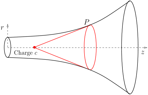
Figure 4: The ”near vortex” approximation.

Then we find the magnetic field that is generated by a charge $c$ at the tip of the cone

$$|\vec{B}|=\frac{c}{d^{2}}=c\left(\frac{f^{\prime}}{f}\right)^{2}\frac{1}{1+\left(\frac{rf^{\prime}}{f}\right)^{2}}\ .$$ (3.4)

where $d$ is the distance from a generic point $(z,r)$ on the red surface to the tip of the cone. In order to have a constant magnetic flux as we vary $z$, the charge $c$ must be a function of $z$. The magnetic flux is

$$\Phi_{B}=\int B_{z}=2\pi\int_{0}^{f^{\prime}}dr\,rc\left(\frac{f^{\prime}}{f}\right)^{2}\frac{1}{\left(1+\left(\frac{rf^{\prime}}{f}\right)^{2}\right)^{3/2}}~{}.$$ (3.5)

Performing the integral we finally obtain:

$$\Phi_{B}=2\pi c\left(1-\frac{1}{\sqrt{1+{f^{\prime}}^{2}}}\right)~{}.$$ (3.6)

This expression gives us the function $c(z)$. The magnetic field in the point $P$ is what we need for the differential equation (3.2). To obtain it we just take (3.4) evaluated at $r=f(z)$. The function $c(z)$ is given by (3.6) where we have also to remember that in our rescaled unit where the radius of the vortex is $1$ and the magnetic field inside is $1$, the magnetic flux is $\pi$. Finally the differential equation (3.2) becomes:

$$-\frac{f^{\prime}{}^{4}}{4f^{4}\left(1+f^{\prime 2}\right)\left(\sqrt{1+f^{\prime 2}}-1\right)^{2}}+\rho\frac{1+f^{\prime 2}-~{}f^{\prime\prime}f}{f(1+f^{\prime 2})^{3/2}}+(1-\rho)=0~{}.$$ (3.7)

As we mentioned before this differential equation is only an approximation. The procedure we have used to compute the magnetic field is not exact but becomes reliable when the surface is very well approximated by a cone. This means that the quantity $ff^{\prime\prime}$ must be very small. Near the vortex the second derivative $f^{\prime\prime}$ is very small and thus we can use the ordinary differential equation (3.7) to understand the physical properties of the junctions near the vortex.

Now we take a look at the solutions to the differential equation. From now on we use $\rho=1$ that means only tension and zero energy density. In Figure 5 we have the two fundamental junctions: (A) is a vortex connected to a domain wall and (B) a vortex that ends on a point. Since this point must be a source of magnetic flux, we can call it a monopole. In Figure 6 we have more general junctions: (C) is a wall-vortex-wall, (D) is a monopole-vortex-wall, (F) monopole-vortex-monopole.

Figure 5: The orbits.

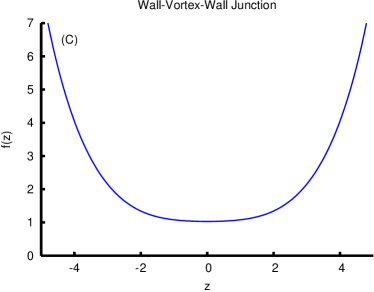
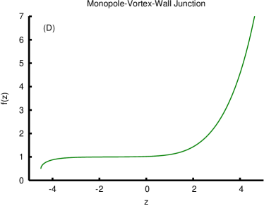
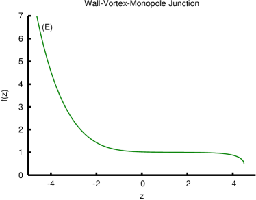
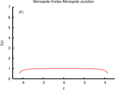
Figure 6: More general junctions.

The overall picture becomes more clear if we consider the differential equation (3.7) as a dynamical system. This means simply that we rewrite the second order differential equation in the following way

$$\left\{\begin{array}[c]{r@{\hspace{1.5pt}}l}f^{\prime}\hskip&=g\\ g^{\prime}\hskip&=\mathcal{F(}f,g\mathcal{)}\end{array}\right.\ ,$$ (3.8)

where $\mathcal{F(}f,g\mathcal{)}$ is just what remains if we isolate $f^{\prime\prime}$ in the differential equation (3.7). The differential equations (3.8) are a simple example of a dynamical system. We have a phase space $(f,g)$ and a flow defined on it. The time of the flow is in this case the $z$ coordinate. The vortex is the fixed point of the flow $f=1$ and $g=0$. To understand the physical behavior around the fixed point we make a Taylor expansion

$$\left(\begin{array}[c]{c}f^{\prime}\\ g^{\prime}\end{array}\right)=\left(\begin{array}[c]{cc}0&1\\ 3&0\end{array}\right)\left(\begin{array}[c]{c}f-1\\ g\end{array}\right)+\dots$$ (3.9)

The diagonalization leads to

$$\left(g\pm\sqrt{3}\left(f-1\right)\right)^{\prime}=\pm\sqrt{3}\left(g\pm\sqrt{3}\left(f-1\right)\right)+\dots$$ (3.10)

What we read from this is the following. The vortex is a stationary point of the dynamical system. The linear expansion shows that this is a saddle point. The solutions of Figure 5 (with the corresponding $z\rightarrow-z$ reflected ones) are the orbits that at $z\rightarrow-\infty$ ($z\rightarrow\infty$) go into the vortex. The orbits around the vortex are the two lines (3.10) $g=\pm\sqrt{3}\left(f-1\right)$. If we draw the solutions in a phase plot we obtain Figure 7.

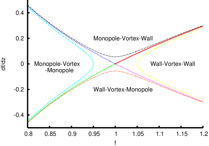
Figure 7: The phase diagram $(f,f^{\prime})$ around the stationary point $(1,0)$.

3.2 Flux tube, domain wall and monopole ($\rho=1$)

The first junction we want to study is the flux tube that ends on a domain wall. In this case we have to take $\rho=1$ so the Higgs phase and the Coulomb phase are both true vacua of the theory.

First we want determine the coefficient of the logarithmic deformation of the wall when a vortex is attached to it. What we are going to describe is summarized in Figure 8.

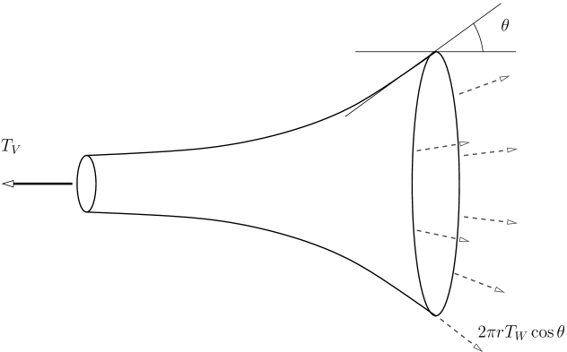
Figure 8: Asymptotic behavior of the logarithmical bending.

The piece of junction in the figure has two forces that acts on it. The first is the vortex that pulls it down with a tension $T_{V}$. The second is the wall that pulls it up. These two forces must be equal:

$$T_{\mathrm{V}}=2\pi rT_{\mathrm{W}}\frac{1}{\sqrt{1+{\tan{\theta}}^{2}}}\ ,$$ (3.11)

where $\tan{\theta}=\mathrm{d}r/\mathrm{d}z$. At the end we obtain a differential equation for the profile $r(z)$:

$${r^{\prime}(z)}^{2}-(2\pi T_{\mathrm{W}}/T_{\mathrm{V}})^{2}{r(z)}^{2}+1=0\ .$$ (3.12)

This equation can be trusted only at large $r$. In fact in making the balance of the forces we have not considered the magnetic field inside the wall. For large $r$ its contribution is negligible since $B$ fall offs as $1/r^{2}$ which implies that the energy density $B^{2}r^{2}$ falls of as $1/r^{2}$. Anyway (3.12) gives the correct coefficient of the logarithmic bending at large $r$:

$$z\simeq\frac{T_{\mathrm{V}}}{2\pi T_{\mathrm{W}}}\log{r}+\cos t\ .$$ (3.13)

Since $\frac{T_{\mathrm{V}}}{2\pi T_{\mathrm{W}}}=\frac{3}{2}R_{\mathrm{V}}$, and we are choosing units in which $R_{\mathrm{V}}=1$, this means that the vortex-wall junction asymptotically goes like

$$r\propto e^{\frac{2}{3}z}~{}.$$ (3.14)

Now it is time to finally compute the vortex-wall junction. The strategy we use is the following. Eqs. (3.10) and (3.14) give us the asymptotic behavior of the profile function at $z\rightarrow-\infty$ (near the vortex) and $z\rightarrow+\infty$ (near the wall). We construct a trial function with the desired asymptotic behaviors and with a certain number of free parameters. These parameters will be adjusted by our numerical code in order to approximate in the best possible way the “real” vortex-wall solution. The more the free parameters are the bigger is the space of profile functions that our trial function can span. For any given choice of the parameters we have a certain profile function and we can thus solve the Laplace equation (2.12) and the mechanical forces. To solve the Laplace equation we use a finite element method routine. Once we have the mechanical force and the magnetic force for a given profile we can compute the total force that is just the sum of the two. For the “real” vortex-wall junction the two forces must be exactly equal but opposite in direction in every point on the profile (2.13). For our trial function we thus compute the norm of the total force (the integral of the total force squared) and then minimize it. The minimization gives, within the space spanned by our trial functions, the best approximation to the real junction. For the vortex-wall junction the result of the computation is given in Figure 9. We show both the junction and the force diagram.

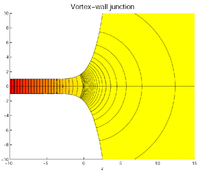
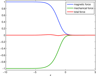
Figure 9: Vortex-wall junction and its force plot ($\rho=1$).

We have used the same strategy to compute the vortex-monopole junction. The result is given in Figure 10.

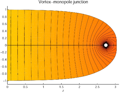
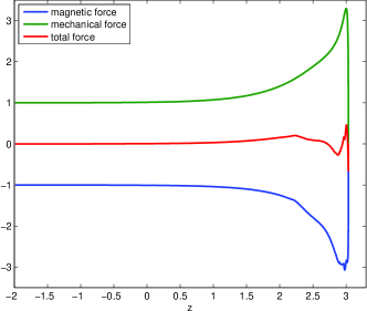
Figure 10: Vortex-monopole junction and its force plot ($\rho=1$).

We can finally plot the global phase diagram in Figure 11.

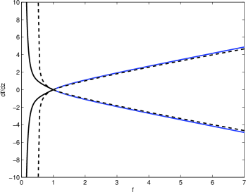
Figure 11: Phase diagram for $\rho=1$. The dashed lines correspond the near vortex approximation given in Figure 7.

3.3 Flux tube, domain wall and monopole ($\rho<1$)

Now we want to study the same junctions in the case $\rho<1$. We can expand the “near vortex” approximation (3.7) around the stationary point $(1,0)$ and we obtain

$$\left(\begin{array}[c]{c}f^{\prime}\\ g^{\prime}\end{array}\right)=\left(\begin{array}[c]{cc}0&1\\ \frac{4-\rho}{\rho}&0\end{array}\right)\left(\begin{array}[c]{c}f-1\\ g\end{array}\right)+\dots$$ (3.15)

The diagonalization leads to

$$\left(g\pm\sqrt{\frac{4-\rho}{\rho}}\left(f-1\right)\right)^{\prime}=\pm\sqrt{\frac{4-\rho}{\rho}}\left(g\pm\sqrt{\frac{4-\rho}{\rho}}\left(f-1\right)\right)+\dots$$ (3.16)

And so the orbits around the vortex are the two lines $g=\pm\sqrt{\frac{4-\rho}{\rho}}\left(f-1\right)$.

The first junction we want to study is the vortex-wall. In the case $\rho<1$ the energy density of the Coulomb vacuum is not zero and this means that a stable domain wall does not exist. On the other hand we have a beautiful solution for the vortex-wall junction in the case $\rho<1$ in Figure 12. What happens to this solution when $\rho$ is decreased? The fact is that a vortex-wall junction can exist if the two dimensional space orthogonal to the vortex is compactified. If we compactify the two dimensional space on a circle then its radius $R_{\mathrm{Max}}$ is given by

$$T_{\mathrm{V}}=\frac{\Phi_{B}^{2}}{2\pi R_{\mathrm{V}}^{2}}+T_{\mathrm{W}}2\pi R_{\mathrm{V}}+\varepsilon_{0}\pi R_{\mathrm{V}}^{2}\ =\frac{\Phi_{B}^{2}}{2\pi R_{\mathrm{Max}}^{2}}+\varepsilon_{0}\pi R_{\mathrm{Max}}^{2}~{}.$$ (3.17)

The previous equation is simply the balance of forces. The tension of the vortex, that is equal to the sum of the magnetic field, wall and bulk energies, must be equal to the tension in the Coulomb vacuum that is given only by the magnetic field and the energy density. With our units ($\Phi_{B}=\pi,T_{\mathrm{W}}=\frac{\rho}{2},\varepsilon_{0}=\frac{1-\rho}{2}$) the radius $R_{\mathrm{Max}}$ is determined by the following equation

$$\pi\left(1+\frac{\rho}{2}\right)=\frac{\pi}{2R_{\mathrm{Max}}^{2}}+\frac{1-\rho}{2}\pi R_{\mathrm{Max}}^{2}~{}.$$ (3.18)

For the vortex-wall junction the result of the computation is given in Figure 12.

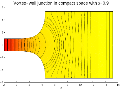
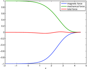
Figure 12: Vortex-wall junction and its force plot ($\rho=0.9$).

The last junction is the vortex-monopole junction for the case $\rho<1$. This junction is the most difficult to compute and is also the one where we have reached least precision. The difficult part comes from the shape of the wall vortex surface around the point where it intersects the axial line $r=0$. Due to symmetry reasons the magnetic field in this point must be zero so the total mechanical force must be zero. In the case $\rho=1$ the Coulomb energy density $\varepsilon_{0}$ is zero and so also the curvature of the wall vortex surface must be zero (see Figure 10). When the Coulomb energy density $\varepsilon_{0}$ is not zero and it exerts a force that tends to retreat the surface. The two radia of curvature are equal, directed outwards and with modulus given by

$$2\frac{T_{\mathrm{W}}}{R_{\mathrm{Curv}}}=\varepsilon_{0}\ ,$$ (3.19)

that in our units means

$$R_{\mathrm{Curv}}=\frac{2\rho}{1-\rho}~{}.$$ (3.20)

For the vortex-monopole junction the result is given in Figure 13.

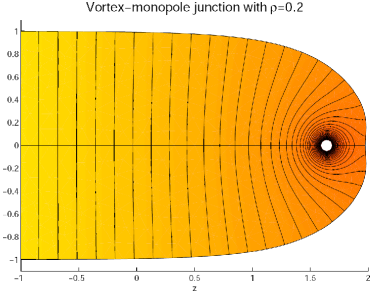
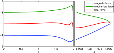
Figure 13: Vortex-monopole junction and its force plot ($\rho=0.2$).

We also plot the global phase for $\rho=0.2$ in Figure 14.

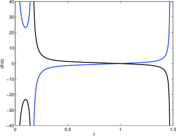
Figure 14: Phase diagram for $\rho=0.2$.

4 Conclusions and Discussions

We conclude the paper with a discussion on possible generalizations and physical applications of the junctions of large $n$ vortices.

4.1 Soliton junctions and dynamical systems   

One interesting outcome of this paper is the relation between soliton junctions and a dynamical system (see [33] for an introduction to the subject). Considering $z$ as the time of the dynamical system, the flux tube is a stationary point of the differential equation. The linear expansion around it shows that this is a saddle point where two lines of orbits intersect. Now think about the junction with a vortex in the middle, for example the wall-vortex-wall or the monopole-vortex-monopole. We can have a lot of this kind of junctions since the length of the vortex in the middle can be fixed at pleasure. From the dynamical system point of view this is very simple to understand. Since the vortex is a saddle point we can have orbits that goes arbitrarily near to the vortex and then escape.

In the analysis of Subsection 3.1 we have a very simple dynamical system. The phase space is two dimensional and consist of the profile $f(z)$ and its derivative $f^{\prime}(z)$. Now suppose we are dealing with a non-large $n$ vortex. The phase space will be an infinite dimensional space This is the space of the field configurations $q(r,z)$ and $A_{i}(r,z)$ and their derivatives. Even in this infinite dimensional space we can think of the vortex as a stationary saddle point of the dynamical system. The fact that the vortex is a saddle point is just a consequence of the $z\rightarrow-z$ reflection symmetry. If we make a linearization around a stationary point and we have a subspace $H^{(-)}$ of orbits that go to the vortex solution at $z\rightarrow-\infty$, we also have a mirror symmetric subspace $H^{(+)}$ of orbits that go to the vortex solution at $z\rightarrow+\infty$.

The theory of dynamical systems is a very vast and evolutes branches of mathematics. What we have used in this paper is just a tiny bit of it. A lot of interesting phenomena arise in the study of the global properties of the dynamical systems. It would be interesting to adopt this point of view in the study of soliton junctions in more sophisticated theories.

4.2 Web of flux tubes  

It is possible to relax the condition of cylindrical symmetry and look for generic stationary configurations of the wall vortex surface. Consider first the case of the junction between three flux tubes. A vortex that carries $n$ units of flux can be split into two vortices with fluxes $n_{1}$ and $n_{2}$ where $n=n_{1}+n_{2}$. As long as $\rho$ is different from zero, the vortices are of type I and this means that the tensions satisfy the inequality $T_{1}+T_{2}>T$. A non-trivial junction between the three vortices is thus possible and the angles are uniquely determined by the tensions. If $\rho=0$ the angle between the two smaller vortices is zero and so the junction is trivial. It is nevertheless possible to obtain a four-vortex junction.  With these basic junctions we can construct a web of flux tubes in three dimensions.

The master equations (2.12) and (2.13) can be generalized relaxing the condition of cylindrical symmetry. We have to take a map from a generic punctured oriented two dimensional surface to the three dimensional space. The punctures on the surface are mapped to the flux tubes at infinity and every handle correspond to an additional flux tube in the web. The master equation is now a system of two partial differential equations. The first one is just the Laplace equation (2.12) for magnetic scalar potential inside the tubes (with the correct boundary conditions) and the other one is the balance of forces

$$-\left.\frac{B^{2}}{2}\right|_{\mathrm{wall}}+\frac{T_{\mathrm{W}}}{R_{1}}+\frac{T_{\mathrm{W}}}{R_{2}}+\varepsilon_{0}=0~{},$$ (4.1)

where now $R_{1}$ and $R_{2}$ are the two radia of curvature of the surface.

4.3 Confining strings

A possible physical application of large $n$ vortices is in the context of confining strings in large $N$ gauge theories (see [28] and [30] for reviews). We briefly review the hypothesis pointed out in [2] which is the following. Consider an $SU(N)$ pure gauge theory and denote by $k$-string the string that confines two heavy probes quark and anti-quark in the $k$-index antisymmetric representation. We then consider the saturation limit that is the limit where we send both $k$ and $N$ to infinity keeping fixed the ratio $x=k/N$. The large $N$ limit is as usual accompanied by the ’t Hooft rescaling of the coupling constant $g^{2}=\widetilde{g}^{2}N$. A useful physical quantity is the ratio of string tensions divided by $N$

$$\mathcal{R}(x,N)=\frac{1}{N}\frac{T(k,N)}{T(1,N)}~{}.$$ (4.2)

$\mathcal{R}(x,N)$ is the a quantity with a smooth saturation limit. Now comes an assumption. Inside the ${\EuFrak{su}}(N)$ Lie algebra there is a particular generator, that up to gauge invariance is unique, that exponentiated passes trough all the elements of the center of the gauge group. We assume that the $k$-strings are a sort of dual vortices of this $U(1)$. This is of course a non-proved assumption but the nice thing, as we are going to see, is that it has a very clear signal that can be tested with lattice computations [29]. The fact is that the string tension must now satisfy two constraints. The first is that in the free string limit ($k$ fixed while $N$ goes to infinity) the tension must be linear in $k$ plus subleading corrections. On the other hand, based on the assumption we just made, the tension for the dual $U(1)$ vortex must also be linear when $k$ is large. The only reasonable way to combine these two limits is that $\mathcal{R}(x,N)$ in the saturation limit is the triangular function plus subleading corrections.

$$\mathcal{R}(x,N)=\min{(x,1-x)+}\mathcal{O(}1/N\mathcal{)}~{}.$$ (4.3)

If this turns out to be correct, the vortex-monopole junction studied in the present paper will be a good description of the $k$-string quark junction and will maybe be visible in lattice computations with a large number of colors.

5 Acknowledgments

We thank K. Konishi for useful comments and for the precious collaboration to the initial stages of the work. We thank also D.Tong for a useful discussion. The work of S.B. supported by the Marie Curie Excellence Grant under contract MEXT-CT-2004-013510.

References

- [1] S. Bolognesi, “Domain walls and flux tubes,” Nucl. Phys. B 730, 127 (2005) [arXiv:hep-th/0507273].
- [2] S. Bolognesi, “Large N, Z(N) strings and bag models,” Nucl. Phys. B 730, 150 (2005) [arXiv:hep-th/0507286].
- [3] S. Bolognesi and S. B. Gudnason, Nucl. Phys. B 741 (2006) 1 [arXiv:hep-th/0512132].
- [4] A. A. Abrikosov, “On The Magnetic Properties Of Superconductors Of The Second Group,” Sov. Phys. JETP 5 (1957) 1174 [Zh. Eksp. Teor. Fiz. 32 (1957) 1442]. H. B. Nielsen and P. Olesen, “Vortex-Line Models For Dual Strings,” Nucl. Phys. B 61, 45 (1973).
- [5] W. A. Bardeen, M. S. Chanowitz, S. D. Drell, M. Weinstein and T. M. Yan, “Heavy Quarks And Strong Binding: A Field Theory Of Hadron Structure,” Phys. Rev. D 11 (1975) 1094.
- [6] A. Chodos, R. L. Jaffe, K. Johnson, C. B. Thorn and V. F. Weisskopf, “A New Extended Model Of Hadrons,” Phys. Rev. D 9 (1974) 3471. K. Johnson and C. B. Thorn, “String - Like Solutions Of The Bag Model,” Phys. Rev. D 13, 1934 (1976).
- [7] M. Shifman and A. Yung,“Domain walls and flux tubes in N = 2 SQCD: D-brane prototypes,” Phys. Rev. D 67 (2003) 125007 [arXiv:hep-th/0212293].
- [8] N. Sakai and D. Tong,“Monopoles, vortices, domain walls and D-branes: The rules of interaction,” JHEP {0503} (2005) 019 [arXiv:hep-th/0501207].
- [9] R. Auzzi, M. Shifman and A. Yung,“Studying boojums in N = 2 theory with walls and vortices,” Phys. Rev. D 72 (2005) 025002 [arXiv:hep-th/0504148].
- [10] A. Hanany and D. Tong, “Vortices, instantons and branes,” JHEP 0307 (2003) 037 [arXiv:hep-th/0306150].
- [11] R. Auzzi, S. Bolognesi, J. Evslin, K. Konishi and A. Yung, “Nonabelian superconductors: Vortices and confinement in N = 2 SQCD,” Nucl. Phys. B 673 (2003) 187 [arXiv:hep-th/0307287]; R. Auzzi, S. Bolognesi, J. Evslin and K. Konishi,“Nonabelian monopoles and the vortices that confine them,” Nucl. Phys. B 686 (2004) 119 [arXiv:hep-th/0312233].
- [12] R. Auzzi, S. Bolognesi and J. Evslin,“Monopoles can be confined by 0, 1 or 2 vortices,” JHEP 0502 (2005) 046 [arXiv:hep-th/0411074].
- [13] D. Tong, “Monopoles in the Higgs phase,” Phys. Rev. D 69 (2004) 065003 [arXiv:hep-th/0307302].
- [14] M. Shifman and A. Yung, “Non-Abelian string junctions as confined monopoles,” Phys. Rev. D 70 (2004) 045004 [arXiv:hep-th/0403149].
- [15] J. P. Gauntlett, R. Portugues, D. Tong and P. K. Townsend, “D-brane solitons in supersymmetric sigma-models,” Phys. Rev. D 63 (2001) 085002 [arXiv:hep-th/0008221].
- [16] J. P. Gauntlett, D. Tong and P. K. Townsend, “Multi-domain walls in massive supersymmetric sigma-models,” Phys. Rev. D 64 (2001) 025010 [arXiv:hep-th/0012178].
- [17] Y. Isozumi, M. Nitta, K. Ohashi and N. Sakai, “Construction of non-Abelian walls and their complete moduli space,” Phys. Rev. Lett. 93 (2004) 161601 [arXiv:hep-th/0404198].
- [18] Y. Isozumi, M. Nitta, K. Ohashi and N. Sakai, “All exact solutions of a 1/4 Bogomol’nyi-Prasad-Sommerfield equation,” Phys. Rev. D 71 (2005) 065018 [arXiv:hep-th/0405129].
- [19] M. Eto, Y. Isozumi, M. Nitta, K. Ohashi, K. Ohta, N. Sakai and Y. Tachikawa, “Global structure of moduli space for BPS walls,” Phys. Rev. D 71 (2005) 105009 [arXiv:hep-th/0503033].
- [20] D. Tong, “D-branes in field theory,” JHEP 0602 (2006) 030 [arXiv:hep-th/0512192].
- [21] M. Shifman and A. Yung, “Bulk-brane duality in field theory,” arXiv:hep-th/0603236.
- [22] M. Eto, T. Fujimori, Y. Isozumi, M. Nitta, K. Ohashi, K. Ohta and N. Sakai, “Non-Abelian vortices on cylinder: Duality between vortices and walls,” Phys. Rev. D 73 (2006) 085008 [arXiv:hep-th/0601181].
- [23] E. Witten, “Branes and the dynamics of QCD,” Nucl. Phys. B 507 (1997) 658 [arXiv:hep-th/9706109].
- [24] A. Hanany, M. J. Strassler and A. Zaffaroni, “Confinement and strings in MQCD,” Nucl. Phys. B 513 (1998) 87 [arXiv:hep-th/9707244].
- [25] S. Bolognesi and J. Evslin, “Stable vs unstable vortices in SQCD,” JHEP 0603 (2006) 023 [arXiv:hep-th/0506174].
- [26] D. Tong, “TASI lectures on solitons,” arXiv:hep-th/0509216.
- [27] M. Eto, Y. Isozumi, M. Nitta, K. Ohashi and N. Sakai, “Solitons in the Higgs phase: The moduli matrix approach,” arXiv:hep-th/0602170.
- [28] J. Greensite, “The confinement problem in lattice gauge theory,” Prog. Part. Nucl. Phys. 51, 1 (2003) [arXiv:hep-lat/0301023].
- [29] B. Lucini, M. Teper and U. Wenger, “Glueballs and k-strings in SU(N) gauge theories: Calculations with improved operators,” JHEP 0406 (2004) 012 [arXiv:hep-lat/0404008].
- [30] A. Armoni and M. Shifman, “Remarks on stable and quasi-stable k-strings at large N,” Nucl. Phys. B 671 (2003) 67 [arXiv:hep-th/0307020].
- [31] A. Vilenkin and E. P. S. Shellard, “Cosmic Strings And Other Topological Defects”, Cambridge University Press.
- [32] J. D. Jackson, “Classical Electrodynamics”, Wiley.
- [33] D. K. Arrowsmith and C. M. Place, “An Introduction to Dynamical Systems”, Cambridge University Press.