Discreteness and the origin of probability in quantum mechanics

Abstract

Attempts to derive the Born rule, either in the Many Worlds or Copenhagen interpretation, are unsatisfactory for systems with only a finite number of degrees of freedom. In the case of Many Worlds this is a serious problem, since its goal is to account for apparent collapse phenomena, including the Born rule for probabilities, assuming only unitary evolution of the wavefunction. For finite number of degrees of freedom, observers on the vast majority of branches would not deduce the Born rule. However, discreteness of the quantum state space, even if extremely tiny, may restore the validity of the usual arguments.

I Introduction: the problem with probability

Quantum mechanics exhibits an odd dichotomy in the time evolution of states. A quantum state undergoes deterministic, unitary evolution until a measurement causes probabilistic, non-unitary collapse. While many physicists do not feel that there is anything wrong with this standard Copenhagen picture, it seems less than economical to postulate two fundamental processes—unitary evolution and non-unitary measurement—if somehow one could suffice. Everett Everett proposed that unitary time evolution of a closed system is sufficient to account for the appearance of measurement collapse to observers inside the system (see also Hartle Hartle and DeWitt and Graham DeWitt ), in what has now become known as the Many Worlds (MW) formulation of quantum mechanics.

The MW interpretation is regarded as extravagant, and hence implausible, by many (including at least one of the authors), because of the huge multiplicity of branches of the wavefunction, each of which is presumed to be as real as the others fn1 . Before the anti-MW reader abandons this paper, we note that the discussion that follows applies also to the conventional Copenhagen interpretation, with measurement collapse, and may allow a derivation of probability in quantum mechanics from a weaker initial assumption, known as the certainty assumption, along the lines of Hartle Hartle (see also Farhi, Goldstone and Gutmann Farhi and Coleman and Lesniewski CL ). An attractive doctrine (preferred by one of the authors) is the minimalist view outlined by Hartle Hartle2 insisting that physics should be done without ill-defined words and slogans such as “The other worlds are just as real.” Our analysis could also be read within this post-Everett or decoherent histories approach.

We focus on the Born rule in quantum mechanics, and the extent to which it can be derived. The Born rule states that given an observable $A$ with spectrum $\lambda_{i}$ and eigenstates $|\psi_{i}\rangle$, the probability of $\lambda_{i}$ as the outcome of a measurement on state $|\psi\rangle$ is $P_{i}=|\langle\psi_{i}|\psi\rangle|^{2}$. It has been claimed by Everett, Hartle, and others, that this rule arises as a consequence of the assumption of unitary evolution, but as we discuss below, the derivation is unsatisfactory for any system with only a finite number of degrees of freedom. (For recent discussions of the Born rule in MW, see others .)

In a recent paper BHZ we speculated that quantum gravity and related considerations may imply that quantum state space is itself discrete. We will review our argument in the next section. Here we point out that one consequence of this discreteness in state space may be the emergence of the Born rule, even in the case when the number of degrees of freedom is finite.

The original derivation of the Born rule given by Everett Everett , Hartle Hartle , and others, is quite simple. Consider an ensemble of identically prepared states

$$\varPsi=\psi\otimes\cdots\otimes\psi=\otimes_{a=1}^{N}~{}\psi^{(a)},$$ (1)

and a sequence of outcomes $S=(s_{1},s_{2},\ldots,s_{N})$ obtained from measurements on each of the states. The probability $P(S)$ of a given sequence, or class of sequences, calculated using the Born rule, is identical to the norm (magnitude) squared of the projection of $\varPsi$ onto eigenstates with the eigenvalues $(s_{1},s_{2},\ldots,s_{N})$, namely $|\langle s_{1}s_{2}\ldots s_{N}|\varPsi\rangle|^{2}$. As Everett noted, it follows that an improbable sequence corresponds to a component of $\varPsi$ (in the eigenstate basis) with small magnitude. In the formal limit $N\rightarrow\infty$, components of $\varPsi$ which do not correspond to statistically typical sequences generated by the Born rule have zero magnitude (i.e. converge to the null vector), and therefore do not correspond to physical states. From the frequentist perspective on probability, then, the Born rule is a consequence of excluding zero norm states from the Hilbert space.

To further elucidate, consider a simple example using spin states. Let $|\psi\rangle=c_{+}|+\rangle+c_{-}|-\rangle$, and define $p_{\pm}=|c_{\pm}|^{2}$. Then a sequence of measurement outcomes will be of the form $S=\{++-+\cdots\}$. If the sequence is generated by the Born rule, then in the limit of large $N$, the fraction of $(+)$ outcomes will be $p_{+}$ to very good approximation. Any other value for the fraction of $(+)$ outcomes has zero probability at infinite $N$. Correspondingly, the magnitude squared $|\langle s_{1}s_{2}\cdots s_{N}|\varPsi\rangle|^{2}$ is zero for any state $\langle s_{1}s_{2}\cdots s_{N}|$ in which the fraction of outcomes $s_{i}$ equal to $(+)$ is not $p_{+}$.

This can be generalized: if $\langle s_{1}s_{2}\cdots s_{N}|$ corresponds to a sequence $S=\{s_{1},s_{2},\ldots,s_{N}\}$ which is statistically atypical according to the Born rule, its overlap with $\varPsi$ will vanish when $N\rightarrow\infty$. Everett referred to these branches of the wavefunction as “maverick worlds”—observers on these branches would not deduce the Born rule. Below, we will repeat this discussion for those readers who prefer a more standard Copenhagen interpretation to the MW interpretation.

We can define parameters characterizing the deviation of a maverick world from the central Born value. For example, in the spin example, we might consider $f_{+}$ to be the frequency of $(+)$ outcomes, so that $\delta=f_{+}-p_{+}$ is the deviation parameter. Then any branch with non-zero $\delta$ will have vanishing norm in the large $N$ limit. When $N$ is strictly infinite all maverick worlds have zero norm. The remaining branches have outcomes $S$ which satisfy the Born rule in the frequentist sense.

The problem with this reasoning is of course that $N$ is never strictly infinite. In fact, given the finite size of the causal horizon of our universe and an ultraviolet cutoff on modes (e.g., from the Planck scale), we obtain a finite, although very large, upper limit on the number of outcomes $N$ which characterize any particular branch of the MW wavefunction. Without invoking something like the Born rule—a correspondence between probability and norm—there is no reason to exclude branches with small but non-zero norm. The problem is exacerbated by the fact that maverick worlds are generally far more numerous than non-maverick worlds. The MW wavefunction branches with each measurement, regardless of how small either of $|c_{\pm}|^{2}$ is. This leads to $2^{N}$ total branches after $N$ measurements. Even if, e.g., $|c_{+}|^{2}$ is much larger than $|c_{-}|^{2}$, both $(+)$ and $(-)$ outcomes will still occur at each branch, and the structure of the tree is independent of $c_{\pm}$ as long as neither is zero. The overwhelming majority of branches will have roughly equal numbers of $(+)$ and $(-)$ outcomes. Thus the multiplicity of maverick worlds is enormously larger than non-maverick worlds, although their collective magnitude is vanishingly small. Again, without assuming the Born rule, we have no à priori reason to exclude small (but non-zero) norm states.

Of course, a strict frequentist interpretation of probability requires an infinite sequence of outcomes. However, the use of probability by physicists is more Bayesian than frequentist: confronted with a finite sequence of outcomes, $S=(s_{1},s_{2},\ldots,s_{N})$, our goal is to deduce a predictive model for subsequent outcomes. In this way, we deduce the Born rule based on the limited number of measurements thus far performed on quantum systems.

As mentioned, our discussion may be of interest even to those who do not accept MW, as it pertains to the origin of the Born rule within the Copenhagen, or measurement collapse, interpretation. In particular, it has been proposed by Hartle Hartle that the Born rule can be derived from the weaker certainty assumption, stating that when a measurement of an observable $A$ is performed on an eigenstate $|a\rangle$ of $A$, the value $a$ is obtained with certainty. Taking $A$ to be, for example, the frequency operator for $(+)$ outcomes, or any other statistical property, Hartle found that for $N$ infinite, $\varPsi$ is an eigenstate of each of these statistical operators, with eigenvalues given by the Born rule.

The discussion parallels that in the MW interpretation. In the standard Copenhagen picture the state $\varPsi$ is, in the eigenstate basis, a sum of $2^{N}$ terms, each term being in one-to-one correspondence with a MW branch or a universe. In the Copenhagen interpretation the outcomes $S$ result from measurements on an ensemble, whereas in MW they specify a particular branch or decoherent history dh of the wavefunction of the entire universe. The mathematics is the same in either picture: maverick terms collectively have a very small norm that approaches zero as $N$ approaches infinity.

This has the same weakness as the earlier MW argument. For any finite $N$, the state $\varPsi$ is only approximately an eigenstate of the frequency operator. The certainty assumption does not specify the outcome of a measurement on an approximate eigenstate, and going further requires an assumption relating the norm of a state vector to the probability of a measurement outcome, which is essentially the Born rule.

II Discrete state space

Consider normalized states $\varPsi=\psi\otimes\cdots\otimes\psi$ and $\varPsi^{\prime}=\psi^{\prime}\otimes\cdots\otimes\psi^{\prime}$. Suppose that, due to fundamental discreteness, one cannot distinguish $\psi$ and $\psi^{\prime}$ when $|\,\psi-\psi^{\prime}|<\epsilon$. This implies that the direct product states cannot be distinguished when (assuming $\sqrt{N}\epsilon\ll 1$)

$$|\,\varPsi-\varPsi^{\prime}|<\sqrt{N}\epsilon.$$ (2)

(We have assumed that $\langle\psi|\psi^{\prime}\rangle$ is real, which would be the case if $\psi^{\prime}$ resulted from rotating $\psi$ slightly on the Bloch sphere. Relative phases could lead to order $N\epsilon$ terms in Eq. (2), which allow an acceptable cutoff of maverick branches for even smaller discreteness scale $\epsilon$.) Motivated by this observation, we assume that any (maverick!) components of $\varPsi$ with norm less than $\sqrt{N}\epsilon$ can be removed from the wavefunction.

We argued in Ref. BHZ that quantum gravity suggests a discreteness scale of order $\epsilon\sim E$, where $E$ is the characteristic energy of the system described by $\psi$, in Planck units. Equivalently, $\epsilon\sim L^{-1}$, where $L$ is the characteristic size, or Compton wavelength, of the system. We can motivate this result by noting that quantum gravity seems to imply a minimal length minlength of order the Planck length. A minimal length restricts our ability to distinguish two different orientations of an experimental apparatus, such as a Stern-Gerlach device for measuring the orientation of a spin. (Rotation of the device by an angle less than $L^{-1}$ does not displace any component by more than the Planck length.) Thus, the resulting ambiguity in the spin state even after an ideal measurement is at least of order $\epsilon$ given above (see Fig. 1). There is no way to ensure that the ensemble states $\psi$ are identical to accuracy better than $\epsilon$. For example, each time we pass a spin through the Stern-Gerlach device to produce another $\psi$ there can be no guarantee that the Stern-Gerlach device remains in precisely the same orientation.

While some might consider fundamental discreteness of the space of quantum states (previously referred to in the earlier paper BHZ as discrete Hilbert space fn2 ) to be a radical notion, we find asserting its absolute continuity in the absence of any supporting experimental evidence to be perhaps just as speculative. Consider the case of spacetime: few would claim that spacetime must be absolutely continuous (in fact, most likely it is not minlength ); why should quantum state space be different?

It is worth emphasizing that the discreteness we propose has nothing to do with the dimensionality of state space. Rather, it has to do with whether the coefficients $c_{i}$ in an eigenstate expansion $|\psi\rangle=\sum_{i}c_{i}|i\rangle$ are continuous or can only take on a discrete set of values (see Fig. 1).

We have not specified the concrete realization of discreteness, other than to assume that states can be defined only modulo some fundamental uncertainty. There are many ways to define the evolution of a state in a discrete state space. One method would be to write the time evolution operator $e^{-iHt}$ as a product of discrete evolution operators $e^{-iH\Delta t}$ and apply this product of operators sequentially to the state, followed by the “snap to” rule (“snap to nearest lattice site”; see Fig. 1) after each step. This is equivalent to taking classical digital computer simulations literally. That is, by accepting the finite precision of the variable $\psi(x)$ in an ordinary computer program, one obtains a naive discretization of Hilbert space with the “snap to” rule implemented by simple numerical rounding. With limited numerical precision, branches of the wavefunction with very small norm are eventually discarded. This scheme leads to small violations of linear superposition, but only at the level of $\epsilon$.

Interestingly, for $\epsilon\sim L^{-1}$, the condition that discreteness have only a small effect on $\varPsi$, $\sqrt{N}\epsilon\ll 1$, leads to a condition on the number of degrees of freedom reminiscent of holography h1 :

$$N\ll L^{2}\sim A,$$ (3)

where $A$ is the surface area of the region. This bound implies far fewer degrees of freedom than the usual extensive scaling $N\sim L^{3}$. It can be deduced as a constraint from gravitational collapse h2 . Excluding states from the Hilbert space of the $L^{3}$ volume which would have already caused gravitational collapse to a black hole, we find the stronger condition $N<A^{3/4}\sim L^{3/2}$.

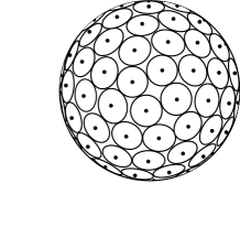
Figure 1: A possible discretization of the Bloch sphere (qubit state space). Points on each disc (of size $\epsilon$) are identified. Points between discs can be assigned to the nearest disc.

III No maverick worlds

Consider the spin example from the first section. Let $n=n_{+}=f_{+}N$ be the number of $(+)$ outcomes in the sequence $S$. We suppress the $+$ subscript in what follows. For $N\gg 1$, the function

$$P(n)=\genfrac{(}{)}{0.0pt}{}{N}{n}\,p^{n}(1-p)^{N-n}.$$ (4)

has a sharp maximum at $n=pN$ and rapidly decreases for $n$ sufficiently far from it. The maximum results from a competition between the combinatorial factor (multiplicity), which is peaked at $n=N/2$, and the product $p^{n}(1-p)^{N-n}$, which is peaked at either $n=0$ or $n=N$, unless $p_{-}$ is extremely close to $p_{+}$. It follows that when calculating $P(n)$ for $n$ not too far from $pN$, we make a negligible error by assuming $n\gg 1$ and $N-n\gg 1$. The Stirling formula gives

$$P(fN)\approx\left[2\pi Nf(1-f)\right]^{-1/2}\exp\left[-N\phi(f)\right],$$ (5)

where

$$\phi(f)=f\ln{(f/p)}+(1-f)\ln{[(1-f)/(1-p)]}$$ (6)

and $f=n/N$. For large $N$ this becomes sharply peaked. Expanding $\phi(f)$ around $f=p$, we find

$$P(fN)\approx\left[2\pi Np(1-p)\right]^{-1/2}\exp\left[-\frac{N(f-p)^{2}}{2p(1-p)}\right].$$ (7)

The collective magnitude squared of all maverick states $|\delta,N\rangle$ with frequency deviation $|\delta|=|f-p|$ greater than $\delta_{0}$ is

$$\sum_{|\delta|>\delta_{0}}\langle\delta,N|\delta,N\rangle\approx 2N\int_{p+\delta_{0}}^{\infty}df~{}P(fN)~{}.$$ (8)

One contribution to the sum comes from the range $f\in[0,p-\delta_{0}]$ and the other from the range $f\in[p+\delta_{0},1]$. Note that we have replaced $f(1-f)$ in the overall factor in $P(fN)$ by $p(1-p)$. The resulting error should be negligible for our purposes here.

Requiring that this collective magnitude squared is less than $N\epsilon^{2}$ yields

$$\delta_{0}>N^{-1/2}\left[2p(1-p)|\ln(N\epsilon^{2})|\right]^{1/2}.$$ (9)

The maximum deviation $\delta$ for undiscarded branches vanishes as $N\rightarrow\infty$ for fixed $p,\epsilon$. If, for finite $N$, an experimenter could measure all $N$ outcomes which define his branch of the wavefunction, he might find a deviation from the predicted Born frequency $f=p$ as large as $|\ln(N\epsilon^{2})|^{1/2}$ standard deviations (i.e., measuring the deviation in units of $N^{-1/2}$). Note that we are working in the regime $N\epsilon^{2}\ll 1$. If the discussion in Ref. BHZ offers a valid guide, the number $\epsilon$ may be much smaller than $10^{-20}$, so that even if $N$ is as large as Avogadro’s number, $N\epsilon^{2}$ will still be a small number (see example below).

However, an experimenter is unlikely to be able to measure more than a small fraction of the outcomes that determine his branch. Recall that in MW a particular branch of the wavefunction is specified by the sequence of outcomes $S=(s_{1},s_{2},\ldots,s_{N})$. $N$ is the total number of decoherent outcomes on a branch, so it is typically enormous—at least Avogadro’s number if the system contains macroscopic objects such as an experimenter. The experimental outcomes available to test Born’s rule will be a much smaller number $N_{*}\ll N$ corresponding to a subset of the $s_{i}$ directly related to the experiment. Any deviation from the Born rule of order $N^{-1/2}$ will be well within the experimental statistical error of order $N_{*}^{-1/2}$. Therefore the Born rule will be observed to hold in all the branches which remain after truncation due to discreteness. This would, however, not be true if we were to set $\epsilon$ to zero, in which case $|\ln(N\epsilon^{2})|^{1/2}$ would be infinite.

For definiteness, consider the following numerical example. Let the discreteness scale be truly tiny: $\epsilon\sim 10^{-100}$, and let $N\sim 10^{160}$, which is the Hubble four-volume in fermis. Then $|\ln(N\epsilon^{2})|^{1/2}\sim 10$, so unless experimenters can measure more than $10^{-2}N\sim 10^{158}$ quantum outcomes, they will have insufficient statistics to exclude any of the maverick branches which remain after truncation.

IV Copenhagen again

If we assume the Copenhagen (collapse) interpretation, our analysis describes when the Born rule can be supplanted by the weaker assumption of certainty of measurement outcome when the measured state is an eigenstate. In a discrete Hilbert space it is natural to extend the notion of eigenstate, so that states within the discreteness distance $\epsilon$ of an eigenstate will also be considered eigenstates. (More precisely, we cannot distinguish between any two such states.) As discussed in the previous section, for large (but finite) $N$, $\varPsi$ is approximately an eigenstate of any statistical operator (such as the frequency operator, but also higher moments) with eigenvalue equal to the Born rule value. For example, the wavefunction is sharply peaked at the Born rule frequency value of $f=p$. If, motivated by the discreteness scale $\epsilon$, we simply modify the certainty assumption to include states which are approximate eigenstates, we will have deduced the Born rule from a more elementary assumption.

There is, however, a technical difficulty in defining how close a state $\varPsi$ is to being an eigenstate of an operator such as the frequency operator. It would be natural to impose a certainty criteria as follows. Given $\varPsi$ satisfying

$$|\varPsi-\varPsi_{f}|<\sqrt{N}\epsilon~{},$$ (10)

where $\varPsi_{f}$ is an eigenstate of the frequency operator with eigenvalue $f$, we identify $\varPsi$ with $\varPsi_{f}$ and require that a measurement of the frequency on $\varPsi$ return the value $f$ with certainty. The problem arises because, for finite $N$, no choice of $\varPsi=\otimes_{a=1}^{N}\psi^{(a)}$ is an exact eigenstate of the frequency operator (except in the trivial cases where $\psi$ is already an eigenstate such as $|+\rangle$ or $|-\rangle$, and in those cases $f$ is either zero or one). The state $\varPsi_{f}$ does not exist, except in the limit $N\rightarrow\infty$, so the distance criteria in Eq. (10) cannot be defined. ($\varPsi$ and $\varPsi_{f}$ live in Hilbert spaces of very different dimensions.) One has to rely on some other criterion for identifying a state $\varPsi$ as a frequency eigenstate.

One possibility is to use the width of $|\varPsi|^{2}$ about the maximum, in comparison to some $\epsilon$-dependent quantity. When the width is sufficiently small, the certainty assumption is assumed to apply. Consider a self-adjoint operator $A$, its eigenvectors $\psi_{i}$ and eigenvalues $\lambda_{i}$, $A\psi_{i}=\lambda_{i}\psi_{i}$, $\langle\psi_{i}|\psi_{j}\rangle=\delta_{ij}$ ($i,j=1,\ldots,n$). (For the qubit case $A$ is the spin operator and $n=2$.) For a state $\psi=\sum_{i=1}^{n}c_{i}\psi_{i}$, projection operators $P_{i}$ satisfy $P_{i}\psi=c_{i}\psi_{i}$. This gives $\langle\psi|P_{i}|\psi\rangle=|c_{i}|^{2}=p_{i}$ and $\sum_{i=1}^{n}p_{i}=1$. Let us consider the state of $N$ copies of $\psi$, $\varPsi=\otimes_{a=1}^{N}\psi^{(a)}$. The frequency operators for the eigenvalues $\lambda_{i}$ are

$$F_{i}=N^{-1}\sum_{j_{1},\ldots,j_{N}=1}^{n}\sum_{a=1}^{N}\delta_{ij_{a}}\otimes_{b=1}^{N}P_{j_{b}}.$$ (11)

We find

$$\langle\varPsi|F_{i}|\varPsi\rangle=p_{i},$$ (12)

$$\langle\varPsi|F_{i}^{2}|\varPsi\rangle=N^{-1}p_{i}+N^{-1}(N-1)p_{i}^{2},$$ (13)

and the variances are $(\Delta F_{i})^{2}=N^{-1}p_{i}(1-p_{i})$.

Consider $\psi^{\prime}=\sum_{i=1}^{n}c^{\prime}_{i}\psi_{i}$ close to $\psi$, and require

$$(p_{i}-p^{\prime}_{i})^{2}<\text{min}\{(\Delta F_{i})^{2},(\Delta F^{\prime}_{i})^{2}\}.$$ (14)

This gives

$$|c_{i}-c^{\prime}_{i}|^{2}<N^{-1}(1-p_{i}),$$ (15)

which leads to

$$|\psi-\psi^{\prime}|^{2}<N^{-1}(n-1).$$ (16)

This condition is satisfied if we require $|\psi-\psi^{\prime}|^{2}\ll\epsilon^{2}$, recalling that $N\epsilon^{2}<1$. It is natural to identify the two states $\psi$ and $\psi^{\prime}$, and consider them both approximate eigenstates of the frequency operator.

V Conclusions

We argued that attempts to derive the Born rule, either in the Many Worlds or Copenhagen interpretation, are unsatisfactory for systems with only a finite number of degrees of freedom. For Many Worlds this is a serious problem, since its goal is to account for apparent collapse phenomena—including the Born rule for probabilities—assuming only unitary evolution of the wavefunction. For finite number of degrees of freedom, observers on the vast majority of branches would not deduce the Born rule.

However, we noted that discreteness of the quantum state space, even if extremely tiny, may restore the validity of the usual arguments. Some may regard discreteness as a radical proposal. We might argue that it is actually less speculative than absolute continuity, something that can never be experimentally verified.

VI acknowledgements

S. H. thanks R. Hanson and J. Hormuzdiar for stimulating his interest in this topic. The authors thank J. Hartle and S. Weinberg for encouraging comments. A. Z. is particularly indebted to J. Hartle for an enlightening discussion of the decoherent history approach as described in Ref. Hartle2 . S. H. and R. B. are supported by the Department of Energy under DE-FG06-85ER40224, while A. Z. is supported in part by the National Science Foundation under grant number PHY 04-56556.

References

- (1) H. Everett, Rev.Mod.Phys 29 3 454 (1957)
- (2) J.B. Hartle, Am. J. Phys. 36 704 (1968)
- (3) B. S. DeWitt and N. Graham in The Many Worlds Interpretation of Quantum Mechanics, Princeton University Press (1973).
- (4) J.B. Hartle, [gr-qc/9210006].
- (5) The MW formalism is familiar to anyone who studies quantum computation. A quantum computer is an isolated system which evolves according to a unitary quantum algorithm during a computation. A description of the state of the quantum computer during the computation involves a wavefunction with many branches, and no collapse until the final read-out of the results. MW proposes that the entire universe should be treated like a quantum computer; a brain only perceives what appears to be a measurement collapse as it becomes correlated with an outcome on a particular branch of the wavefunction, and decoheres from other branches due to vanishing overlap. Those who do not accept MW are either asserting that: (i) quantum mechanics is incomplete or (ii) our brains cannot be simulated by sub-components of a quantum computer, which do split into multiple branches. In case (i), quantum computers will, perhaps at some threshold of complexity, fail to operate as predicted. Case (ii) also denies the possibility of conventional artificial intelligence, since quantum computers can simulate classical Turing machines.
- (6) E. Farhi, J. Goldstone and S. Gutmann, Annals Phys. 192, 368 (1989).
- (7) S. Coleman and A. Lesniewski, unpublished.
- (8) D. Deutsch, Proc. R. Soc. Lond. A455, 3129 (1999); H. Barnum, C.M. Caves, J. Finkelstein, C.A. Fuchs and R. Schack, Proc. R. Soc. Lond., A456, 1175 (2000); W. Zurek, Phys. Rev. Lett. 90, 120404 (2003); Rev. Mod. Phys. 75, 715 (2003), Phys. Rev. A 71, 052105 (2005); R. Hanson, Found. Phys. 33,1129 (2003), Proc. R. Soc. Lond., A462, 1619 (2006).
- (9) R. V. Buniy, S. D. H. Hsu and A. Zee, Phys. Lett. B 630, 68 (2005) [hep-th/0508039].
- (10) M. Gell-Mann and J. B. Hartle, Phys. Rev. D 47, 3345 (1993) [gr-qc/9210010].
- (11) X. Calmet, M. Graesser, S. D. H. Hsu, Phys. Rev. Lett. 93:211101, (2004) [hep-th/0405033], Int. J. Mod. Phys. D 14, 2195 (2005) [hep-th/0505144].
- (12) It has not escaped our notice that discrete Hilbert space is something of an oxymoron, given the mathematical properties of a Hilbert space. However, the identification of quantum state space and Hilbert space in physics has become so strong that the two are almost interchangeable in the minds of physicists.
- (13) L. Susskind, J. Math. Phys. 36, 6377 (1995), [hep-th/9409089]; J. M. Maldacena, Adv. Theor. Math. Phys. 2, 231 (1998), [hep-th/9711200].
- (14) G. ’t Hooft, [gr-qc/9310026]; R. V. Buniy and S. D. H. Hsu, [hep-th/0510021].