FTPI-MINN-06-17

UMN-TH-2504-06

Domain Lines as Fractional Strings

R. Auzzi${}^{\,a}$, M. Shifman${}^{\,a}$ and A. Yung${}^{\,a,b,c}$

^aWilliam I. Fine Theoretical Physics Institute, University of Minnesota, Minneapolis, MN 55455, USA
^bPetersburg Nuclear Physics Institute, Gatchina, St. Petersburg 188300, Russia
^cInstitute of Theoretical and Experimental Physics, Moscow 117250, Russia

We consider $\mathcal{N}=2$ supersymmetric quantum electrodynamics (SQED) with 2 flavors, the Fayet–Iliopoulos parameter, and a mass term $\beta$ which breaks the extended supersymmetry down to $\mathcal{N}=1$. The bulk theory has two vacua; at $\beta=0$ the BPS-saturated domain wall interpolating between them has a moduli space parameterized by a $U(1)$ phase $\sigma$ which can be promoted to a scalar field in the effective low-energy theory on the wall world-volume. At small nonvanishing $\beta$ this field gets a sine-Gordon potential. As a result, only two discrete degenerate BPS domain walls survive. We find an explicit solitonic solution for domain lines — string-like objects living on the surface of the domain wall which separate wall I from wall II. The domain line is seen as a BPS kink in the world-volume effective theory. We expect that the wall with the domain line on it saturates both the $\{1,0\}$ and the $\{\frac{1}{2},\frac{1}{2}\}$ central charges of the bulk theory. The domain line carries a magnetic flux which is exactly $\frac{1}{2}$ of the flux carried by the flux tube living in the bulk on each side of the wall. Thus, the domain lines on the wall confine charges living on the wall, resembling Polyakov’s three-dimensional confinement.

1 Introduction

Supersymmetric gauge theories were shown to support a large variety of extended critical (i.e. BPS-saturated) objects exhibiting various nontrivial dynamical patterns. In particular, gauge theories with extended $\mathcal{N}=2$ supersymmetry (SUSY) present a unique framework in which many strong-coupling problems can be modeled and addressed in a quantitative way. The most famous example of this type is the Seiberg–Witten solution [1, 2].

In the last few years we witnessed extensive explorations of various $\mathcal{N}=2$ models at weak coupling. Solitonic BPS-saturated objects of novel types were found and studied, such as non-Abelian flux tubes (strings) [3, 4], domain-wall junctions [5, 6, 7, 8, 9], domain-wall-string junctions (boojums) [10, 11, 12, 13, 14], trapped monopoles [15, 16, 17] and so on, for recent reviews see [13, 18, 19]. Instantons inside domain walls in five dimensions have been discussed recently in Ref. [20].

In this paper we construct another, so far unknown, example of a composite BPS soliton — strings lying on domain walls. These strings carry one half of the magnetic flux of the bulk strings (hence, the name “fractional”). From 3D perspective of the wall world-volume theory they are akin to Polyakov’s confining strings of (1+2)-dimensional compact electrodynamics [21]. A crucial element of our construction is the fact of the gauge field localization on the wall observed in [10] (a mechanism of such localization was first discussed in [22]).

If we consider two distinct isolated supersymmetric vacua, a domain wall configuration interpolating between them always exists. Moreover, sometimes there is more than one interpolating configuration; all of them must have one and the same tension, as the walls under consideration are BPS-saturated. Such a situation can happen if the wall has a continuous modulus or moduli (in addition to the translational modulus), which can be promoted to field(s) living on the wall world-volume, see e.g. [10].

Another possibility is that just a finite number of domain walls exist interpolating between the two given vacua. The first example of this type, two distinct walls, was found in SU(2) SQCD [23]. In [24] it was argued that in SU($N$) super-Yang–Mills with $\mathcal{N}=1$ the number of distinct “minimal” domain walls between vacua in any given pair of “adjacent” vacua is $N$. A weak coupling analysis can be carried out by passing to a weakly coupled Higgs phase through addition of fundamental matter (see Refs. [25, 26]).

Given the existence of a finite number of non-gauge-equivalent walls connecting two given bulk vacua, it is natural at this point to address the problem of domain lines, which are junctions between two of the above walls. In this paper this problem is addressed in the controllable regime of weak coupling. From the bulk perspective the domain lines to be analyzed below can be viewed as bulk strings put on the brane, see Fig. 1. Since these domain lines carry magnetic flux they are of an explicitly different class than those discussed in [26].

Where does the magnetic flux come from? In SQED per se one can introduce magnetic monopoles à la Dirac, as probe external objects. Alternatively, we could embed the U(1) theory in the ultraviolet in an SU(2) gauge theory, with SU(2) being spontaneously broken down to U(1) at some high scale. Then the magnetic charges would appear as the ’t Hooft–Polyakov monopoles. Since the electric charges are condensed in both vacua, to the left and to the right of the wall, a magnetic charge placed in the bulk would form a flux tube, which would go to the wall in the perpendicular direction. On the wall world-volume this tube splits in two distinct domain lines. Each of them carries a half of the monopole magnetic flux. Since we have two distinct domain lines, it is possible to build a static configuration where the monopole is represented by a junction of the two domain lines. This is conceptually similar to the confined monopoles of Refs. [15, 16, 17, 27, 28]. Thus, the monopoles can be trapped not only by non-Abelian strings — they can be nested inside the walls too!

Our basic bulk model is $\mathcal{N}=2$ SQED with $N_{f}=2$ flavors and the Fayet–Iliopoulos (FI) parameter $\xi$. This is the model used in [10], where the reader can find all relevant details. In $\mathcal{N}=2$ SQED there are two equivalent ways of introducing the FI parameter: through the $D$-term and through superpotential [29, 30]. We will introduce $\xi$ in the superpotential, along with a small mass parameter $\beta$ breaking $\mathcal{N}=2$ down to $\mathcal{N}=1$. We will work in the limit

$$\xi\gg m_{A},\,\,\beta\,,\qquad A=1,2\,,$$ (1)

where $m_{A}$ are the mass parameters of the two matter hypermultiplets. An effective Lagrangian emerging at low energies is that of the sigma model with the Eguchi–Hanson manifold as the target space. The domain walls at $\beta=0$ in this problem were studied previously in [31, 32].

The theory at $\beta=0$ has a moduli space of BPS walls which can be parameterized by a phase $\sigma$,

$$0<\sigma<2\pi\,.$$

This is due to the fact that the symmetry of the bulk theory is U(1)$\times$U(1). In each vacuum the local U(1) gets Higgsed while the other one remains unbroken. However, it is spontaneously broken on the wall [10]. At $\beta=0$ the (probe) magnetic charges, monopoles, are confined in the bulk since their magnetic flux gets squeezed into the Abrikosov–Nielsen–Olesen (ANO) flux tubes [33]. Inside the wall the charged matter condensates vanish, and the magnetic flux can spread all over the brane, so that the probe magnetic charges on the wall world-volume are in the Coulomb phase. This is the mechanism responsible for localization of a gauge field on the domain wall.

Indeed, the scalar $\sigma$ can be dualized à la Polyakov [21] into a gauge vector on the wall world-volume. The field strength tensor is given by (see e.g. Ref. [10]):

$$F^{(2+1)}_{nm}=\frac{e^{2}_{2+1}}{2\pi}\,\epsilon_{nmk}\,\partial^{k}\sigma\,.$$ (2)

The end-point of the ANO string on the wall becomes a dual electric charge, the source of the dual electric field in Eq. (2) which, in the original description, was the magnetic field.

Now, what happens if we deform the above theory by switching on $\beta\neq 0\,$?

Once we introduce a small $\beta$ perturbation (we will consistently work in the first nontrivial order in $\beta$), the main impact on the bulk theory is an explicit breaking of the global U(1). As a result, the modulus $\sigma$ ceases to be a massless field. A potential of the form

$$V=\frac{\beta^{2}\xi}{m}\,\cos^{2}\sigma+\mathcal{O}(\beta^{3})$$ (3)

develops. The interaction (3) is nonlocal in terms of the dual vector field (2).

The potential (3) lifts the moduli space leaving us with two isolated vacua, at $\sigma=\pi/2$ and $\sigma=3\pi/2$. Thus, we have two degenerate BPS domain walls to be referred to as walls of type I and type II. The domain line is a “wall on a wall”, it divides the the wall into two domains – one in which we have the type I wall from another of type II wall. In terms of the effective world-volume description the domain line is a sine-Gordon kink in the effective world-volume theory (3). The sine-Gordon potential we obtain at $\beta\neq 0$ is in one-to-one correspondence with Polyakov’s sine-Gordon potential [21]. There are three nuances, though: (i) Polyakov’s potential is generated by instantons of the compact 3D electrodynamics; (ii) in our case we deal with $\mathcal{N}=1$ sine-Gordon, while Polyakov’s model was not supersymmetric; (iii) the flux tube in Polyakov’s model was unique, while we have two distinct types, see below.

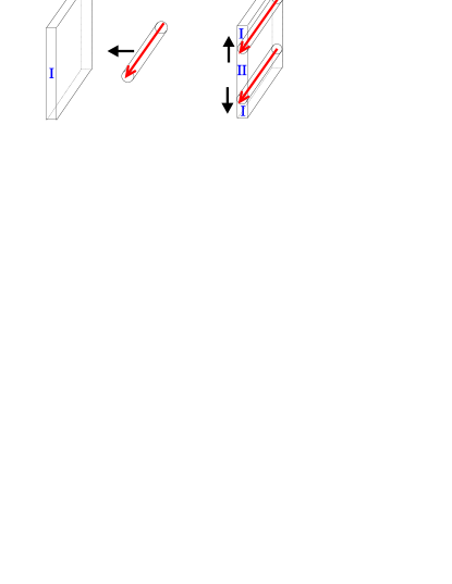
Figure 1: The fate of the bulk flux tube parallel to a nearby domain wall of type I. In the bulk the string tension is of order $\xi$ while on the wall of order $\xi\beta/m$. So for small $\beta$ the vortex is attracted by the wall. On the wall world-volume the string is a composite Sine-Gordon double kink; two Sine-Gordon kinks repel each other and so a region of type II domain wall will appear in between. At $\beta=0$ the kink disappears and the vortex just annihilates due to the fact that magnetic charges are in Coulomb phase on the wall world-volume.

With the potential (3) generated, the Coulomb-like picture of the dual field flux lines disappears, since the flux gets collimated inside the domain lines. Note that in three dimensions there exist two distinct ways in which long-range gauge potential can acquire a mass gap. First, through a Chern–Simons term

$$S_{\rm CS}=\frac{1}{2\pi}\,\epsilon_{nmk}\,A_{n}\partial_{m}A_{k}\,.$$ (4)

as e.g. in Refs. [24] and [34, 35]. The Chern-Simon term is nonlocal when written in term of the scalar filed $\sigma$. Second, through a sine-Gordon-type potential for $\sigma$ which, in turn, is nonlocal in terms of the dual vector potential.

The organization of the paper is as follows. In Sect. 2 we outline our bulk model and discuss two vacua of the theory. Sect. 3 is devoted to the the sigma-model limit, applicable at $\xi\gg m,\beta$. Here we follow the parameterization introduced in Ref. [32]. Many computations carried out below are simpler in the sigma-model formalism. In Sect. 4.1 the domain walls at $\beta=0$ are reviewed, while in in Sect. 4.2 we address the problem at $\beta\neq 0$. Exact BPS solutions are found in the sigma-model limit for two distinct walls. In Sect. 5 we derive the effective potential for the quasi-modulus $\sigma$ assuming that $\beta$ is small. The potential is found in the leading nontrivial order in $\beta$, namely $\beta^{2}$. In Sect. 6 we discuss the domain lines (2-wall junctions in the nomenclature of Ref. [26]). They are obtained as kinks of the effective world-volume description. We show that there are two types of the domain lines, which thus have a junction of their own. Sect. 7 contains a short summary and conclusions.

2 Theoretical set-up

2.1 Lagrangian of $\mathcal{N}=2$ SQED with two flavors

The bulk theory which we start from has the gauge group U(1)_G, extended $\mathcal{N}=2$ supersymmetry, and $N_{f}=2$ hypermultiplets of matter $\{Q^{A},\,\,\tilde{Q}_{A}\},\,\,\,A=1,2$. We endow it with the Fayet–Iliopoulos parameter $\xi$ in the superpotential. The latter contains the coupling ${\cal A}\sum_{B}\left(Q^{B}\,\tilde{Q}_{B}\right)$ where ${\cal A}$ is the $\mathcal{N}=1$ chiral superfield, the $\mathcal{N}=2$ superpartner of the photon. It also contains the mass term

$$\tilde{Q}_{A}\,{\cal M}^{A}_{B}\,Q^{B}$$ (5)

where ${\cal M}$ is a mass matrix. If the matrix $\mathcal{M}_{ij}$ was Hermitean we could always diagonalize it by unitary transformations of $Q^{A}$ and $\tilde{Q}_{A}$, to obtain a real diagonal matrix. In our case ${\cal M}^{A}_{B}$ is not Hermitean. Without loss of generality we can choose it as follows:

$${\cal M}=\left(\begin{array}[]{c|c}m&-\beta/\sqrt{2}\\ \hline\cr\beta/\sqrt{2}&-m\end{array}\right)\,,$$ (6)

where $m$ and $\beta$ are real and positive parameters. If $\beta=0$ the superpotential (5) is compatible with $\mathcal{N}=2$. If $\beta\neq 0$ we break $\mathcal{N}=2$ supersymmetry down to $\mathcal{N}=1$ once the Fayet–Iliopoulos term is added to the theory. As was mentioned, we assume that $\beta\ll m$.

With these assumptions the superpotential takes the form

$$\mathcal{W}=\frac{1}{\sqrt{2}}\,\mathcal{A}\,Q^{B}\tilde{Q}_{B}+m\left(Q^{1}\tilde{Q}_{1}-Q^{2}\tilde{Q}_{2}\right)+\frac{\beta}{\sqrt{2}}\left(Q^{1}\tilde{Q}_{2}-\tilde{Q}_{1}Q^{2}\right)-\frac{1}{2\sqrt{2}}\,\xi\,\mathcal{A}\,.$$ (7)

The bosonic part of the action can be written as

$$S=\int d^{4}x\left\{\frac{1}{4g^{2}}F_{\mu\nu}^{2}+\frac{1}{g^{2}}|\partial_{\mu}a|^{2}+\bar{\nabla}_{\mu}\bar{q}_{A}\nabla_{\mu}q^{A}+\bar{\nabla}_{\mu}\tilde{q}_{A}\nabla_{\mu}\bar{\tilde{q}}^{A}+V_{D}+V_{F}\right\},$$ (8)

where

$$\nabla_{\mu}=\partial_{\mu}-\frac{i}{2}A_{\mu},\,\,\,\bar{\nabla}_{\mu}=\partial_{\mu}+\frac{i}{2}A_{\mu}\,,$$

and $a$, $q$ and $\tilde{q}$ are the lowest components of the chiral superfields $\mathcal{A}$, $Q$ and $\tilde{Q}$, respectively. Moreover, the potential is the sum of the $D$ and $F$ terms,

$$V_{D}=\frac{g^{2}}{8}\left(|q^{B}|^{2}-|\tilde{q}_{B}|^{2}\right)^{2}\,,$$ (9)

and

$$V_{F}=\frac{1}{2}\left|q^{1}(a+\sqrt{2}m)-\beta q^{2}\right|^{2}+\frac{1}{2}\,\left|\tilde{q}_{2}(a-\sqrt{2}m)-\beta\tilde{q}_{1}\right|^{2}$$

$$+\frac{1}{2}\left|(a+\sqrt{2}m)\tilde{q}_{1}+\beta\tilde{q}_{2}\right|^{2}+\frac{1}{2}\left|(a-\sqrt{2}m)q^{2}+\beta q^{1}\right|^{2}+\frac{g^{2}}{2}\left|\tilde{q}_{A}q^{A}-\frac{\xi}{2}\right|^{2}\,.$$

(10)

At $m=\beta=0$ the theory at hand has two global symmetries: the SU(2)_F flavor symmetry  and the SU(2)_R $R$-symmetry, which is a general feature of $\mathcal{N}=2$ theories.

We pause here to comment on the Fayet–Iliopoulos parameter. One can introduce a generalized Fayet–Iliopoulos term $\vec{\xi}$ (for details see [30]) as a triplet under SU(2)_R. The triplet is formed from the real and imaginary parts of the appropriate $F$-term coefficient in the superpotential (see the last term in Eq. (7)) and the $D$-term coefficient which is real. In this paper we take

$$\hbox{\rm Im}(\xi_{F})=\xi_{D}=0\quad\mbox{ and}\quad\hbox{\rm Re}(\xi_{F})=\xi\,.$$ (11)

We always can bring the Fayet–Iliopoulos parameter to this form by an SU(2)_R rotation. Therefore, our parameter $\xi$ is real; we also assume it to be the largest in the scale hierarchy, $\sqrt{\xi}\gg m/g$. We call $U(1)_{R}$ the $SU(2)_{R}$ subgroup which leaves the Fayet-Iliopolous term in the form of Eq. (11).

The flavor group SU(2)_F is broken down to U(1)_F by the parameter $m\neq 0$; the parameter $\beta\neq 0$ breaks the flavor symmetry completely. Furthermore, SU(2)_R is not broken by $m$ since this mass term preserves $\mathcal{N}=2$. At the same time, SU(2)_R is broken by $\beta\neq 0$. A ${Z}_{2}$ subgroup of U(1)${}_{R}\times$U(1)_F generated by a $\pi$ rotation in both U(1)’s is left unbroken by $\beta$ (this nontrivial property is somewhat hidden in the gauge theory; it becomes more transparent in the sigma-model formalism).

2.2 Two vacua

It is convenient to introduce two parameters,

$$\Omega=\frac{1}{2}\sqrt{\xi+\frac{m\xi}{\sqrt{m^{2}-\beta^{2}/2}}},\qquad\omega=\frac{1}{2}\sqrt{-\xi+\frac{m\xi}{\sqrt{m^{2}-\beta^{2}/2}}}\,.$$ (12)

Note that $\omega=0$ and $\Omega=\sqrt{\frac{\xi}{2}}$ at $\beta=0$.

It is not difficult to see that for $\beta<\sqrt{2}m$ the theory has two vacua. The first vacuum is

$$a=-\sqrt{2m^{2}-\beta^{2}},$$

$$q^{1}=\bar{\tilde{q}}_{1}=\Omega,\quad q^{2}=-\bar{\tilde{q}}_{2}=\omega\,.$$ (13)

The second vacuum is

$$a=\sqrt{2m^{2}-\beta^{2}},$$

$$q^{1}=-\bar{\tilde{q}}_{1}=\omega,\quad q^{2}=\bar{\tilde{q}}_{2}=\Omega\,.$$ (14)

In order to check that the potential vanishes in these vacua we have to use the following arithmetic identity:

$$\sqrt{a\pm\sqrt{b}}=\sqrt{\frac{a+\sqrt{a^{2}-b}}{2}}\pm\sqrt{\frac{a-\sqrt{a^{2}-b}}{2}}\,.$$ (15)

At $\beta=0$ Eqs. (13) and (14) reduce to two vacua considered in [10]. We will be interested in the domain walls interpolating between them.

3 Sigma model description ($\beta,m\ll g\sqrt{\xi}$)

3.1 Constraints and parameters

Under the above choice of parameters we can integrate out the scalar field $a$ and the gauge field. The low-energy effective description is given by a sigma model with the target space on $q^{A},\tilde{q}_{A}$ which is the Eguchi–Hanson manifold defined by the constraints

$$|q^{1}|^{2}+|q^{2}|^{2}=|\tilde{q}_{1}|^{2}+|\tilde{q}_{2}|^{2}\,,\qquad\tilde{q}_{A}q^{A}=\frac{\xi}{2}\,,$$ (16)

in addition, one has to factor out the action of the U(1) gauge group.

A convenient way to parameterize these constraints is explained by Sakai and collaborators in Ref. [32]. Let us introduce the following functions:

$$f(r)=\sqrt{-\frac{\xi}{2}+\sqrt{r^{2}+(\xi/2)^{2}}}\,,\qquad g(r)=\sqrt{\frac{\xi}{2}+\sqrt{r^{2}+(\xi/2)^{2}}}\,.$$ (17)

The Eguchi–Hanson manifold can be parameterized by the radial coordinate $r\geq 0$ plus three angles $\theta,\,\,\psi$ and $\varphi$ with

$$0\leq r<\infty\,,\quad 0\leq\theta\leq\pi\,,\quad 0\leq\varphi\leq 2\pi\,,\quad 0\leq\psi\leq 2\pi\,.$$ (18)

In terms of these functions and angle variables the explicit expression is

$$q^{1} = \frac{e^{i\varphi/2}}{2}\left(e^{i\psi/2}g(r)\cos{\frac{\theta}{2}}+e^{-i\psi/2}f(r)\sin{\frac{\theta}{2}}\right),$$

$$q^{2} = \frac{e^{-i\varphi/2}}{2}\left(e^{i\psi/2}g(r)\sin{\frac{\theta}{2}}-e^{-i\psi/2}f(r)\cos{\frac{\theta}{2}}\right),$$

$$\tilde{q}_{1} = \frac{e^{-i\varphi/2}}{2}\left(e^{-i\psi/2}g(r)\cos{\frac{\theta}{2}}-e^{i\psi/2}f(r)\sin{\frac{\theta}{2}}\right),$$

$$\tilde{q}_{2} = \frac{e^{i\varphi/2}}{2}\left(e^{-i\psi/2}g(r)\sin{\frac{\theta}{2}}+e^{i\psi/2}f(r)\cos{\frac{\theta}{2}}\right).$$ (19)

The generic sections at $r>0$ are three-dimensional submanifolds parameterized by the three angles $\theta,\,\,\varphi$ and $\psi$. The section at $r=0$ is a two-dimensional sphere; only $\theta$ and $\varphi$ are the relevant coordinates here, while the $\psi$-circle shrinks to zero. A compact expression for $r$ in term of the squark vacuum expectation values (VEVs) is

$$\sqrt{4r^{2}+\xi^{2}}=|q^{1}|^{2}+|q^{2}|^{2}+|\tilde{q}_{1}|^{2}+|\tilde{q}_{2}|^{2}\,.$$ (20)

The following formulas are useful, because they readily imply the expressions for the angles $\theta,\,\,\varphi$ and $\psi$ in term of gauge invariant squark bilinears,

$$q^{1}\tilde{q}_{1} = \frac{\xi+\sqrt{4r^{2}+\xi^{2}}\cos\theta}{4}-\frac{ir\sin\theta\sin\psi}{2}\,,$$

$$q^{1}\bar{q}_{2} = \frac{e^{i\varphi}(\xi\sin\theta-2r\cos\theta\cos\psi-2ir\sin\psi)}{4}\,.$$ (21)

3.2 Metric

With this parameterization, the metric is given by the kinetic part of the SQED Lagrangian

$$\mathcal{L}_{\rm k}=-|\partial_{\mu}q|^{2}-|\partial_{\mu}\tilde{q}|^{2}+\frac{i}{2}A_{\mu}\left(\bar{q}\stackrel{{\scriptstyle\leftrightarrow}}{{\partial_{\mu}}}q-\bar{\tilde{q}}\stackrel{{\scriptstyle\leftrightarrow}}{{\partial_{\mu}}}\tilde{q}\right)-\frac{1}{4}A_{\mu}A^{\mu}\left(q\bar{q}+\tilde{q}\bar{\tilde{q}}\right),$$ (22)

where

$$\bar{q}\stackrel{{\scriptstyle\leftrightarrow}}{{\partial_{\mu}}}q=\bar{q}(\partial_{\mu}q)-(\partial_{\mu}\bar{q})q\,.$$ (23)

Since $A_{\mu}$ enters with no derivatives, we can eliminate this field by virtue of the classical equation of motion,

$$A_{\mu}=\frac{i\left(\bar{q}\stackrel{{\scriptstyle\leftrightarrow}}{{\partial_{\mu}}}q-\bar{\tilde{q}}\stackrel{{\scriptstyle\leftrightarrow}}{{\partial_{\mu}}}\tilde{q}\right)}{\bar{q}q+\bar{\tilde{q}}\tilde{q}}\,.$$ (24)

The metric of the low-energy sigma model is (see Ref. [32])

$$\mathcal{L}_{\rm k} = \frac{1}{\sqrt{4r^{2}+\xi^{2}}}\left\{-(\partial_{\mu}r)^{2}-(\partial_{\mu}\theta)^{2}\left(r^{2}+\left(\frac{\xi}{2}\right)^{2}\right)\right.$$

$$- \left.(\partial_{\mu}\varphi)^{2}\left(r^{2}+\left(\frac{\xi}{2}\right)^{2}\sin^{2}\theta\right)-(\partial_{\mu}\psi)^{2}\,r^{2}-(\partial_{\mu}\varphi)\,(\partial_{\mu}\psi)\,(2r^{2}\cos\theta)\right\}.$$

At $\theta=0$ and $\theta=\pi$ there are some singularities in the coordinates (at $\theta=0$ the part of the metric which is bilinear in $d\varphi,d\psi$ is of the form $(d\varphi+d\psi)^{2}$); at $\theta=\pi$ it has the form $(d\varphi-d\psi)^{2}$). Another coordinate singularity takes place at $r=0$, where the coefficients of the bilinears in $d\psi$ vanish. All these singularities are only due to the coordinate choice; the vacuum manifold is smooth everywhere.

3.3 Potential

Now, let us integrate out the gauge field and the scalar field $a$. We observe that the expression for $a$ gets a correction due to $\beta$,

$$a=\frac{\sqrt{2}m\left(|q^{2}|^{2}+|\tilde{q}_{2}|^{2}-|q^{1}|^{2}-|\tilde{q}_{1}|^{2}\right)+\beta\left(\bar{q_{1}}q^{2}-q^{1}\bar{q_{2}}+\tilde{q}_{1}\bar{\tilde{q}}^{2}-\bar{\tilde{q}}^{1}\tilde{q}_{2}\right)}{\sum\left(|q^{A}|^{2}+|\tilde{q}_{A}|^{2}\right)}\,.$$ (26)

Eliminating $A_{\mu}$ and $a$ we get the scalar potential in the form

$$V = \frac{m^{2}(4r^{2}+\xi^{2}\sin^{2}\theta)}{\sqrt{4r^{2}+\xi^{2}}}+2\sqrt{2}m\,\beta\,r\left(\cos\theta\cos\varphi\cos\psi-\sin\varphi\sin\psi\right)$$ (27)

$$+ \frac{\beta^{2}\left(4r^{2}+3\left(\frac{\xi}{2}\right)^{2}+2\xi^{2}\cos 2\theta\left(\sin\varphi\right)^{2}+\xi^{2}\cos 2\varphi\right)}{2\sqrt{4r^{2}+\xi^{2}}}\,.$$

This potential has two vacua, one at $\theta=0$ and $\varphi+\psi=\pi$, the other at $\theta=\pi$ and at $\varphi-\psi=0$ (remember that at $\theta=0,\pi$ it is only a combination of $\varphi,\psi$ that is the coordinate). Both of the vacua are at the same value of $r_{0}$,

$$r_{0}=\frac{\beta\xi}{2\sqrt{2m^{2}-\beta^{2}}}\,.$$ (28)

These are just the vacua discussed in Sect. 2.2 in the sigma-model formalism.

The U(1) rotation of the phase $\varphi$ corresponds to the U(1)_F group of the bulk gauge theory while the rotation of the phase $\psi$ corresponds to U(1)_R. It easy to verify that the part of the potential proportional to $m$ breaks SU(2)${}_{F}\times$U(1)_R down to U(1)${}_{F}\times$U(1)_R. At $\beta=0$ the potential (27) does not depend on $\varphi$ and $\psi$. On the other hand, the part which depends on $\beta$ breaks both U(1) factors. However, a ${Z}_{2}$ subgroup generated by a $\pi$ rotation in both U(1)’s is left unbroken by $\beta\neq 0$.

4 BPS domain walls

4.1 $\beta=0$

First of all let us consider the case $\beta=0,\,\,m\neq 0$. This problem has been studied in detail in Refs. [10, 31, 32], therefore we only briefly review it here.

The ansatz

$$q^{A}=\overline{\tilde{q}_{A}}\equiv\bar{\tilde{q}}^{A}$$

can be used in this case. The BPS equations for the wall are

$$\nabla_{3}q^{1}\pm\frac{1}{\sqrt{2}}\left(q^{1}(\bar{a}+\sqrt{2}m_{1})\right)=0\,,$$

$$\nabla_{3}q^{2}\pm\frac{1}{\sqrt{2}}q^{2}\left(\bar{a}+\sqrt{2}m_{2}\right)=0\,,$$

$$\frac{1}{g}\partial_{3}a\pm\frac{g}{\sqrt{2}}\left(\bar{q}_{B}\,\bar{\tilde{q}}^{B}-\frac{\xi}{2}\right)=0\,.$$ (29)

The tension of the wall $T_{\rm wall}$ is given by the central charge,

$$T_{\rm wall}=2\left|\mathcal{W}({\infty})-\mathcal{W}(-\infty)\right|=2\xi m\,.$$ (30)

This domain wall is a $1/2$ BPS solution of the Bogomol’nyi equations [36]: four of the eight supersymmetry generators of the $\mathcal{N}=2$ bulk theory are broken by the soliton.

The bosonic moduli space is described by two collective coordinates. One of them is of course associated with the translations in the $z$ direction. The other one is a compact U(1) phase parameter $0<\sigma<2\pi$. Indeed, if

$$\{q_{1}(z),\,\,q_{2}(z),\,\,a(z)\}$$

is a solution, we can easily build another solution which is not gauge equivalent, namely

$$\{e^{i\sigma}q_{1}(z),\,\,q_{2}(z),\,\,a(z)\}\,.$$

This is due to a specific feature [10] of the breaking of the U(1)${}_{G}\times$U(1)_F symmetry. In both vacua only one squark develops a VEV, and only one of the two U(1)’s is broken. In each vacuum the phase of the “condensed” squark field is eaten by the Higgs mechanism. On the other hand, on the wall both the U(1)’s are broken — one phase is eaten by the Higgs mechanism, while the other becomes a Goldstone mode localized on the wall.

If we change the relative ratio between $m$ and $\sqrt{\xi}$ the shape of the profiles functions changes. In both limits $m\gg\sqrt{\xi}$ and $m\ll\sqrt{\xi}$ (the sigma-model limit) a simple and compact solution can be found. The $m\gg\sqrt{\xi}$ limit was studied in Ref. [10]. In this case the wall has a three-layer structure: there are two edges of width $\approx 1/\sqrt{\xi}$, where each of the squark VEVs quickly drops to zero, and a large intermediate domain, of width $2m/(g^{2}\xi)$ (see Fig. 2, on the left).

Figure 2: The wall profile functions at $\beta=0$. the plot on the left represents the large $m$ regime (a good approximation is achieved already at $m=3\sqrt{\xi}$); on the right we see the small-$m$ sigma-model regime at $m=0.1\sqrt{\xi}$. The field $q^{1}$ is depicted by blue color, $q^{2}$ by violet and $a$ by red. The units used for $a$ are different from those used for $q^{1}$.

The wall in the sigma-model limit was studied in Refs. [31, 32]. Let us summarize the results of these works, in our notation. The potential is a function only of $r$ and $\theta$, namely,

$$V=\frac{m^{2}\left(8r^{2}+2\xi^{2}\sin^{2}\theta\right)}{\sqrt{4r^{2}+\xi^{2}}}\,.$$ (31)

The two vacua are at $r=0,\,\,\theta=0$ and $r=0,\,\,\theta=\pi$. Indeed, the wall also lives in the $S^{2}$ submanifold at $r=0$. We can use this ansatz (where a profile function $\eta(z)$is introduced for $\theta(z)$) to obtain the following wall equations:

$$q^{1} = \bar{\tilde{q}}^{1}=\sqrt{\frac{\xi}{2}}\left(\cos\frac{\eta(z)}{2}\right)\,,$$

$$q^{2} = \bar{\tilde{q}}^{2}=\sqrt{\frac{\xi}{2}}\left(\sin\frac{\eta(z)}{2}\right)e^{i\sigma}\,,$$

$$a = m\sqrt{2}\left(\sin^{2}\frac{\eta}{2}-\cos^{2}\frac{\eta}{2}\right)=-m\sqrt{2}\,\cos\eta\,.$$ (32)

The profile function $\eta(z)$ is determined by minimization of the following energy functional:

$$\int dz\,\mathcal{H}=\int dz\,\left\{\frac{\xi}{4}\left[(\partial_{z}\eta)^{2}+\sin^{2}\eta\,(\partial_{\mu}\varphi)^{2}\right]+\xi m^{2}\sin^{2}\eta\right\}\,,$$ (33)

which, in turn, implies the BPS equation

$$\eta^{\prime}(z)=2m\sin(\eta(z))\,,$$ (34)

The solution of this equation is

$$\eta(z)=2\arctan\,(\exp(2mz))\,.$$ (35)

A compact expression can be written for the field profiles (see the plot on the right-hand side of Fig. 2),

$$a=\sqrt{2}m\tanh(2mz)\,,$$

$$q^{1}=\bar{\tilde{q}}^{1}=\frac{\sqrt{\xi}}{2}\frac{e^{-mz}}{(\cosh 2mz)^{1/2}}\,,$$

$$q^{2}=\bar{\tilde{q}}^{2}=\frac{\sqrt{\xi}}{2}\frac{e^{mz}}{(\cosh 2mz)^{1/2}}\,.$$ (36)

Note that in the sigma-model limit ($m\ll\xi$ ) the wall thickness $R$ is of the order of $1/m$ (in the $m\gg\xi$ limit it was of the order of $m/(g\sqrt{\xi})$). This is interesting, because this means that $R$ is infinite in both limits: $m\rightarrow 0$ and $m\rightarrow\infty$. This happens because in both limits ($m\to 0$ and $\xi\to 0$) certain states in the bulk theory become light. The minimal wall thickness is at $m=\mathcal{O}(\sqrt{\xi})$, where we cannot use any of the above approximations.

It is possible to promote the moduli parameters to fields depending on the world-volume coordinates. The effective Lagrangian was found in Ref. [10] using an explicit ansatz which takes into account the world-volume dependence of $\sigma$. The bosonic part of the world-volume action is

$$\int d^{3}x\left\{\frac{T_{\rm wall}}{2}\left(\partial_{n}z\right)^{2}+\frac{\xi}{4m}\left(\partial_{n}\sigma\right)^{2}\right\},$$ (37)

where the field $z$ describes the wall position in the perpendicular direction. Furthermore, the phase $\sigma$ can be dualized to a vector field in $(1+2)$ dimensions [21],

$$F^{(2+1)}_{nm}=\frac{e^{2}_{2+1}}{2\pi}\,\epsilon_{nmk}\,\partial^{k}\sigma\,,$$ (38)

where

$$e^{2}_{2+1}=\frac{2\pi^{2}\xi}{m}\,.$$ (39)

Then the bosonic part of the world-volume action takes the form

$$\int d^{3}x\left\{\frac{T_{\rm wall}}{2}\,(\partial_{n}z)^{2}\,-\frac{1}{4e^{2}_{2+1}}(F_{mn}^{2+1})^{2}\right\}.$$ (40)

The full theory is $\mathcal{N}=2$ Abelian gauge theory in three dimensions.

In both vacua of the bulk theory the heavy trial magnetic charges are confined by the Abrikosov–Nielsen–Olesen strings [33]. For example, in the vacuum where $a=-\sqrt{2}m$, the ansatz

$$q^{2}=\tilde{q}_{2}=0\,,\qquad\bar{\tilde{q}}^{1}=q^{1}$$

can be used to derive the following BPS equations for the string:

$$\frac{1}{2}\,\epsilon_{ijk}\,F_{jk}-\frac{g^{2}}{2}\left(|q^{1}|^{2}-\xi\right)=0\,,\qquad\left(\nabla_{1}-i\nabla_{2}\right)q^{1}=0\,.$$ (41)

The string tension is given by the $\{\frac{1}{2},\,\frac{1}{2}\}$ central charge [6]

$$T_{\rm string}=2\pi\xi\,.$$ (42)

The magnetic flux of the minimal-winding flux tube is $4\pi$. Absolutely similar equations can be written in the other vacuum, $a=\sqrt{2}m$. The only difference is that here we now use the ansatz

$$q^{1}=\tilde{q}_{1}=0\,,\qquad q^{2}=\bar{\tilde{q}}^{2}\,,$$

and a nontrivial equation is that for the field $q^{2}$. A BPS configuration exists in which the flux tube is perpendicular to the wall and injects its magnetic flux into the wall (this soliton is called boojum; it is studied in Refs. [10, 11, 13, 14]).

So far, the magnetic field can freely propagate inside the wall. String ends play the role of electric charges in the effective U(1) gauge theory (40) on the wall [10]. They are in the Coulomb phase on the wall world-volume. If we take a flux tube parallel to the wall, it will be attracted to the wall in order to minimize the energy of the configuration. If it reaches the wall it will dissolve, due to the fact that the charges are not confined on the wall.

4.2 Switching on $\beta\neq 0$

We know that if $\beta=0$ there is a moduli space for the BPS walls parameterized by the phase $\sigma$,

$$0\leq\sigma\leq 2\pi\,.$$

Now let us generalize the BPS equations to take into account $\beta\neq 0$. We expect to find just a finite number of BPS wall solutions, because the U(1)${}_{G}\times$U(1)_F symmetry which was responsible for the existence of the continuous modulus $\sigma$ is explicitly broken down to U(1) by the parameter $\beta$. The U(1) phase is eaten up by the Higgs mechanism, and there is no extra global symmetry which can be used in order to build a Goldstone boson localized on the wall.

At $\beta\neq 0$ the ansatz $q^{A}=\bar{\tilde{q}}^{A}$ is no longer satisfied even in the vacua; therefore, it is no more selfconsistent. We have to keep all the squark profiles as independent functional variables. The Bogomolny completion (see Ref. [36]) of the wall energy functional is

$$\int d^{3}x\,\mathcal{H}=\int dx_{3}\left\{\left|\nabla_{3}q^{1}\pm\frac{1}{\sqrt{2}}\left(\bar{\tilde{q}}^{1}\,(\bar{a}+\sqrt{2}m_{1})+\beta\,\bar{\tilde{q}}^{2}\right)\right|^{2}\right.$$

$$+\left|\nabla_{3}\tilde{q}_{1}\pm\frac{1}{\sqrt{2}}\bar{q}_{1}(\bar{a}+\sqrt{2}m_{1})-\beta\,\bar{q}_{2}\right|^{2}+\left|\nabla_{3}q^{2}\pm\frac{1}{\sqrt{2}}\bar{\tilde{q}}^{2}(\bar{a}+\sqrt{2}m_{2})-\beta\,\bar{\tilde{q}}^{1}\right|^{2}$$

$$+\left|\nabla_{3}\tilde{q}_{2}\pm\frac{1}{\sqrt{2}}(\bar{q}_{2}(\bar{a}+\sqrt{2}m_{2})+\beta\,\bar{q}_{1})\right|^{2}+\left|\frac{1}{g}\partial_{3}a\pm\frac{g}{\sqrt{2}}\left(\bar{q}_{B}\,\,\bar{\tilde{q}}^{B}-\frac{\xi}{2}\right)\right|^{2}$$

$$\left.+\partial_{3}\left[\left(\frac{a}{\sqrt{2}}+m_{B}\right)\,q^{B}\tilde{q}_{B}-\frac{\xi a}{2\sqrt{2}}+\frac{\beta\,(q^{1}\,\tilde{q}_{2}-\tilde{q}_{1}\,q^{2})}{\sqrt{2}}\right]\mp{\rm c.c.}\right\}.$$ (43)

The $D$-term constraint is

$$\nabla_{3}\left(|q|^{2}-|\tilde{q}|^{2}\right)^{2}=0\,;$$ (44)

it is recovered as a consequence of the BPS equations (43). The tension of the BPS wall is given by the appropriate central charge,

$$T_{\rm wall}=2\left|\mathcal{W}({\infty})-\mathcal{W}(-\infty))\right|=2\xi\sqrt{m^{2}-\beta^{2}/2}\,.$$ (45)

Figure 3: Plot of the potential at some sections at $r=r_{0}$ and at $\theta=\pi/3,\,\,\pi/2$ and $2\pi/3$. There are always two supersymmetric minima, one at $\phi=\psi=\pi/2$ and the other at $\phi=\psi=3\pi/2$. This is true for all values of $r$ and $\theta$, due to the ${Z}_{2}$ subgroup of U(1)${}_{F}\times$U(1)_R which is left unbroken by $\beta$.

In the gauge-theory approach the solution of the BPS equations are rather contrived. It turns out that the problem is much easier in the sigma model approach. If we plot the potential in different slices at $r,\theta$ constant, we find that there are always two minima, one at $\varphi=\psi=\pi/2$ and the other at $\varphi=\psi=3\pi/2$ (see Fig. 3). Therefore, this is the appropriate ansatz we have to use in order to find two distinct wall solutions. Two profile functions $r(z)$ and $\eta(z)$ are introduced for the sigma-model coordinates $r$ and $\theta$. Then the potential energy is

$$V(r,\eta) = \frac{1}{2\sqrt{4r^{2}+\xi^{2}}}\,\Big{\{}(8m^{2}r^{2}-4\sqrt{2}\,m\,\beta\,r\,\sqrt{4r^{2}+\xi^{2}}$$ (46)

$$+ \beta^{2}\,(4r^{2}+\xi^{2})+(2m^{2}-\beta^{2})\,\xi^{2}\,(\sin\eta)^{2}\Big{\}}\,.$$

At $r=r_{0}$ the part of the potential which is constant in $\eta$ vanishes. In terms of the profile functions the Bogomolny completion of the wall energy is

$$\int d^{3}x\,\mathcal{H} = \int d^{3}x\left\{\left(\frac{\partial_{z}r}{\sqrt[4]{4r^{2}+\xi^{2}}}-\frac{2mr-(\beta/\sqrt{2})\sqrt{4r^{2}+\xi^{2}}}{\sqrt[4]{4r^{2}+\xi^{2}}}\right)^{2}\right.$$ (47)

$$+ \left(\frac{\sqrt[4]{4r^{2}+\xi^{2}}}{2}\,(\partial_{z}\eta)-\frac{\sqrt{m^{2}-\beta^{2}/2}\,\,\xi\sin\eta}{\sqrt[4]{4r^{2}+\xi^{2}}}\right)^{2}$$

$$- \left.\xi\,\sqrt{m^{2}-\beta^{2}/2}\,\,(\partial_{z}\,\cos\eta)\right\}\,.$$

The solution for $r(z)$ is just the constant value $r_{0}$. The solution for $\theta$ is completely similar to the case of vanishing $\beta$,

$$\eta^{\prime}(z) = (2m-\beta^{2}/m)\sin(\eta(z))\,,$$

$$\eta(z) = 2\arctan\,\left[\exp\left((2m-\beta^{2}/m)z\right)\right]\,.$$ (48)

The tension is given by the total derivative term

$$T_{\rm wall}=2\xi\sqrt{m^{2}-\beta^{2}/2}\,,$$ (49)

which, of course, agrees with the result obtained from the central charge of the gauge theory presented in Eq. (45).

At this point we can return to original SQED and write the solutions for the squark fields. For $\phi,\psi=\pi/2$ we have

$$q^{1} = i\Omega\cos(\eta/2)+\omega\sin(\eta/2)\,,\quad q^{2}=i\omega\cos(\eta/2)+\Omega\sin(\eta/2)\,,$$

$$\tilde{q}_{1} = -i\Omega\cos(\eta/2)-\omega\sin(\eta/2)\,,\quad\tilde{q}_{2}=i\omega\cos(\eta/2)+\Omega\sin(\eta/2)$$

$$a = -\sqrt{2m^{2}-\beta^{2}}\left(\cos\eta+i\frac{\beta}{\sqrt{2}m}\sin\eta\right)\,.$$ (50)

Moreover, for $\phi,\psi=3\pi/2$ we have

$$q^{1} = -i\Omega\cos(\eta/2)+\omega\sin(\eta/2)\,,\quad q^{2}=-i\omega\cos(\eta/2)+\Omega\sin(\eta/2)\,,$$

$$\tilde{q}_{1} = i\Omega\cos(\eta/2)-\omega\sin(\eta/2)\,,\quad\tilde{q}_{2}=-i\omega\cos(\eta/2)+\Omega\sin(\eta/2)\,,$$

$$a = -\sqrt{2m^{2}-\beta^{2}}\left(\cos\eta-i\frac{\beta}{\sqrt{2}m}\sin\eta\right)\,.$$ (51)

These solutions correspond to $\sigma=\frac{1}{2}\pi$ and $\sigma=\frac{3}{2}\pi$ of the $\beta=0$ case. We checked by direct substitution that they solve the gauge-theory BPS equations (43) in the limit in which the field $a$ is integrated out (this is a cross-check for our calculations). These wall solutions break spontaneously the ${Z}_{2}$ residual symmetry of the theory at $\beta\neq 0$. This is the reason why we have two distinct walls.

5 Unstable walls

When $\beta\neq 0$ there are just two stable domain wall solutions interpolating between the two vacua of the bulk theory. At generic $\sigma\neq\pi/2$ or $3\pi/2$ we expect that the wall becomes unstable (perhaps, it is better to say, quasistable, at small $\beta$). We will show that from the standpoint of the world-volume theory this can be interpreted as an effective potential with two degenerate minima for the world-volume modulus $\sigma$.

Our purpose is to compute the tension of the unstable walls in the first nontrivial order in $\beta$. The nonconstant part of the wall tension will give us the effective potential of the world-volume effective theory. To this end we have to guess a field configuration which interpolates between the two stable-wall configurations. The following ansatz is a natural extension of the $\beta=0$ case, where the exact answer is known:

$$q^{1} = \frac{e^{i\sigma}\Omega\cos(\eta/2)+\omega\sin(\eta/2)}{A}\,,$$

$$q^{2} = \frac{e^{i\sigma}\omega\cos(\eta/2)+\Omega\sin(\eta/2)}{A}\,,$$

$$\tilde{q}_{1} = \frac{e^{-i\sigma}\Omega\cos(\eta/2)-\omega\sin(\eta/2)}{A}\,,$$

$$\tilde{q}_{2} = \frac{-e^{-i\sigma}\omega\cos(\eta/2)+\Omega\sin(\eta/2)}{A}\,.$$ (52)

As we will show below, the profile function $\eta(z)$ can be identified with the sigma-model coordinate $\theta$ only up to terms of order $\beta^{2}$. The factor $A$ is introduced in order to maintain the sigma-model constraint $|q^{1}|^{2}+|q^{2}|^{2}=|\tilde{q}_{1}|^{2}+|\tilde{q}_{2}|^{2}$. This constraint implies

$$A=\left[\frac{\sqrt{2}m+\beta\sin(\eta/2)\cos\sigma}{\sqrt{2}m-\beta\sin(\eta/2)\cos\sigma}\right]^{1/4}\,.$$ (53)

As will be seen shortly, the above ansatz gives, in the first nontrivial order in $\beta$, an elegant and compact result for the potential.

First of all, let us translate Eqs. (52) and (53) in the sigma-model language. This can be done using the expressions (20) and (21). In the first relevant order in $\beta$ we have

$$r = \frac{\xi\beta}{8m}\sqrt{6+2\cos(2\eta)\cos(2\sigma)+2\cos(2\eta)-2\cos(2\sigma)}+\mathcal{O}(\beta^{2})\,,$$

$$\theta = \eta+\frac{\beta^{2}\cos\eta\sin\eta\cos^{2}\sigma}{4m^{2}}+\mathcal{O}(\beta^{3})\,,$$

$$\phi = \sigma+\mathcal{O}(\beta^{2})\,,$$

$$\sin\psi = \frac{2\sqrt{2}\sin\sigma}{\sqrt{6+2\cos(2\eta)\cos(2\sigma)+2\cos(2\eta)-2\cos(2\sigma)}}+\mathcal{O}(\beta)\,.$$ (54)

The plot of the functions $r(\eta)$ and $\psi(\eta)$ for some values of $\sigma$ is presented in Fig. 4.

Figure 4: Left: $r^{2}(\eta)$ for different values of $\sigma$. At $\sigma=\pi/2$ we have $r$ constant. At $\sigma=0$ and $\eta=\pi/2$ we have $r=0$. Right: $\psi(\eta)$ for different values of $\sigma$. At $\sigma=\pi/2$ we have $\psi$ constant. At $\sigma=0$, $\psi$ tends to a step function, but this is not a problem because $\sigma=0$ we have $r=0$.

We will solve the problem for the effective potential for the modulus $\sigma$ at order $\beta^{2}$. To this end we have to compute the function $\eta(z)$ in the second order in $\beta$. Let us write the energy density as a function of $\sigma$ and $\eta(z)$ in the second order in $\beta$. The kinetic part can be easier found using Eq. (54) in the sigma-model metric (3.2). The kinetic part takes the form

$$\left(\frac{\xi}{4}+\beta^{2}\frac{10+6\cos(2\eta)+2\cos(2\sigma)+6\cos(2\eta)\cos(2\sigma)}{128m^{2}}\right)\left(\frac{d\eta}{dz}\right)^{2}\,.$$ (55)

The potential part can be easier found in the original bulk gauge theory, substituting Eq. (52) in Eq. (10). The potential part is

$$(\sin(\eta))^{2}\left(m^{2}\xi-\frac{\beta^{2}\xi}{32}(10+6\cos(2\eta)-14\cos(2\sigma)+6\cos(2\eta)\cos(2\sigma))\right).$$ (56)

Now, a second order equation can be obtained for the profile function $\eta(z)$,

$$\eta^{\prime\prime}\left(32m^{2}+\beta^{2}(10+6\cos(2\eta)+2\cos(2\sigma)+6\cos(2\eta)\cos(2\sigma))\right)$$

$$+\,4\,\xi m^{2}(\sin 2\eta)\left(-16m^{2}+\beta^{2}(2+6\cos(2\eta)-10\cos(2\sigma)+6\cos(2\eta)\cos(2\sigma))\right)$$

$$\,+\,\eta^{\prime}(24\beta^{2}(\cos\sigma)^{2}\sin 2\eta)=0\,.$$ (57)

We will find the solution to the above equation iteratively in $\beta$. Let us write

$$\eta=\eta_{0}+\beta^{2}\eta_{2}+\mathcal{O}(\beta^{3})\,,$$ (58)

where from Eq. (35) we have

$$\eta_{0}=2\arctan\,(e^{2mz})\,.$$ (59)

Substituting Eqs. (58) and (59) in Eq. (57) we arrive at a linear differential equation for $\eta_{2}$,

$$2\left(\cosh(2mz)\right)^{4}\eta_{2}^{\prime\prime}+4m^{2}\left(\cosh(2mz)\right)^{2}\left(3-\cosh(4mz)\right)\eta_{2}$$

$$+2\sinh(2mz)\left(-2+15(\cos\sigma)^{2}-2\cosh(4mz)\right)=0\,,$$ (60)

which can be readily solved exactly

$$\eta_{2}=-\frac{1}{m^{2}}\,\,\frac{e^{2mz}\left(15\cos^{2}\sigma+8(1+e^{4mz})mz\right)}{4(1+e^{4mz})^{2}}\,.$$ (61)

Note that for $\sigma=\pi/2,\,\,3\pi/2$ Eq. (61) reduces to Eq. (48) in the second order in $\beta$. The final result for $\eta$ thus takes the form

$$\eta(z)=2\arctan(e^{2mz})-\frac{\beta^{2}}{m^{2}}\,\frac{e^{2mz}\left(15\cos^{2}\sigma+8(1+e^{4mz})mz\right)}{4(1+e^{4mz})^{2}}+\mathcal{O}(\beta^{3})\,.$$ (62)

Now we can substitute the solution (62) back in the energy density and integrate in the $z$ direction. In this way we find the tension of the unstable wall at generic values $\sigma$, namely,

$$T_{\rm wall}(\sigma)=2\xi m+\frac{\beta^{2}\xi}{2m}\,\cos(2\sigma)+\mathcal{O}(\beta^{3})\,.$$ (63)

Of course, the minima at $\sigma=1/2\pi,\,\,3\pi/2$ correspond to the two degenerate stable BPS walls. The unstable-wall tension versus $\sigma$ reduces to

$$T_{\rm wall}(\sigma)=T_{\rm wall0}+V(\sigma)+\mathcal{O}(\beta^{3})\,,$$ (64)

where

$$T_{\rm wall0}=2\xi m-\frac{\beta^{2}\xi}{2m}$$ (65)

is the tension of the stable walls (note that this coincides with Eq. (45) in the first order in $\beta^{2}$) and

$$V(\sigma)=\frac{\beta^{2}\xi}{m}\,(\cos\sigma)^{2}$$ (66)

is the world-volume potential for the field $\sigma$. One can (and should) supersymmetrize the world-volume Lagrangian with no difficulty.

6 Domain line as a sine-Gordon kink

The action of the effective theory on the wall world-volume, in the first approximation in $\beta^{2}$, is that of the supersymmetric sine-Gordon model, with 2 supercharges. (We leave aside the translational modulus and its superpartner.) The bosonic part of the Lagrangian (at $\mathcal{O}(1)$ in $\beta$ for the kinetic part and $\mathcal{O}(\beta^{2})$ for the potential) is

$$S=\int d^{3}x\left[\frac{\xi}{4m}(\partial_{n}\sigma)^{2}-\frac{\beta^{2}\xi}{m}\cos^{2}\sigma\right].$$ (67)

We can choose the vacuum at $\sigma=-\pi/2$ as vacuum I and at $\sigma=\pi/2$ as vacuum II (see Fig. 5).

Figure 5: The potential energy for the field $\sigma$ defined on a circle $\sigma\in[0,2\pi)$. The potential energy is presented by the height of the vertical lines. Two minima with the vanishing potential energy are vacua $I$ and $II$, respectively. There are two types of strings in the world-volume theory.

Now it is time to discuss the sine-Gordon kinks interpolating between these two vacua. From Fig. 5 it is obvious that there are two distinct kinks which represent trajectories starting in vacuum I and ending in vacuum II.

Let us denote the world-volume spatial coordinates as $\{x,\,\,y\}$. The domain line is assumed to be oriented in the ${y}$ direction. Therefore the field $\sigma$ in the kink solution will depend on $x$.

The Bogomol’nyi completion of the energy functional can be represented as

$$\mathcal{H} = \int d^{2}x\left(\frac{\xi}{4m}(\partial_{n}\sigma)^{2}+\frac{\beta^{2}\xi}{m}\cos^{2}\sigma\right)$$ (68)

$$= \int d^{2}x\left\{\frac{\xi}{2m}\left(\frac{1}{\sqrt{2}}(\partial_{x}\sigma)\mp\sqrt{2}\beta\cos\sigma\right)^{2}\pm\frac{\xi\beta}{m}\partial(\sin\sigma)\right\}\,.$$

It is not difficult to obtain two distinct kink solutions interpolating between vacuum I and vacuum II,

$$\sigma=2\arctan\,(\exp(2\beta x))-\frac{\pi}{2}\,,$$ (69)

(this solution has $\sigma(x\rightarrow-\infty)=-\pi/2$, $\sigma(x\rightarrow+\infty)=\pi/2$, let us call it $a$-string) and

$$\sigma=-2\arctan\,(\exp(2\beta x))-\frac{\pi}{2}\,,$$ (70)

(this solution has $\sigma(x\rightarrow-\infty)=-\pi/2$, $\sigma(x=+\infty)\rightarrow-3\pi/2$, let us call it $b$-string). Of course, there are two domain lines interpolating between vacuum II and I — antilines — which can be obtained by replacing $x\rightarrow-x$. We denote them as $\bar{a}$ and $\bar{b}$.

The transverse size of these objects is of the order of $1/\beta$ and the tension is

$$T_{\rm dl}=\frac{2\beta\xi}{m}\,.$$ (71)

Note that at this order in $\beta$ the kink is BPS-saturated in the world-volume theory. We expect that the domain line saturates the $\{\frac{1}{2},\,\,\frac{1}{2}\}$ central charge of the $(1+3)$-dimensional theory and that these solitons remain BPS-saturated to all orders in $\beta$.

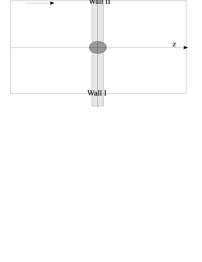
Figure 6: Computation of the domain-line magnetic flux.

From the standpoint of $(1+3)$-dimensional theory the above domain lines are strings each of which carries the magnetic flux that is $1/2$ of the magnetic flux of the flux tube living in the bulk. It is easy to calculate the magnetic flux in the nonsingular gauge; it is given by line integral over the vector potential. Let us consider a rectangular path depicted in Fig. 6. On the left-hand side of the rectangle, at $z\rightarrow-\infty$, we choose $q^{A}=e^{i\sigma(x)}q^{A}_{\rm vac}$ where $q^{A}_{\rm vac}$ are the squark VEVs. On the right-hand side we choose to keep $q^{A}$ constant; on the two horizontal sides we use the gauge in which $A_{z}=0$ (this can be done for each of the wall solutions). In order to keep the covariant derivatives vanishing on the left-hand side we take

$$A_{x}=2\partial_{x}\sigma(x)\,,$$ (72)

where $\sigma(x\rightarrow-\infty)=-\pi/2,\sigma(x\rightarrow+\infty)=\pi/2$ for the $a$-string and $\sigma(x\rightarrow-\infty)=-\pi/2,\sigma(x\rightarrow+\infty)=-3\pi/2$ for the $b$-string. On the other sides we have $A_{k}=0$. The magnetic flux is then given by

$$\mathcal{F}_{\rm dl}=\oint\vec{A}\cdot d\vec{x}=2(\sigma_{x\rightarrow\infty}-\sigma_{x\rightarrow-\infty})=\pm 2\pi,$$ (73)

where the $+$ sign is for the $a$-string and the $-$ sign is for the $b$-string. On the other hand, if we compute in a similar way the flux of the bulk Abrikosov–Nielsen–Olesen string, we find

$$\mathcal{F}_{\rm ANO}=4\pi\,.$$

The two different solutions we obtained — the domain lines $a$ and $b$ — correspond to two possible orientations of the magnetic flux in the ${y}$ direction. An isolated string can not be taken out of the wall, because it connects two different vacua of the wall world-volume theory. On the other hand, if we take a bound state of an $a$-line and a $\bar{b}$-line, this configuration interpolates, through one winding, between one and the the same vacuum of the world-volume theory. Indeed, this bound state carries the same magnetic flux as the flux tube living in the bulk, and, therefore, can be pulled out from the wall. If we take a bound state of an $a$- and $\bar{a}$-lines we get a topologically trivial configuration: $a$ and $\bar{a}$ domain lines annihilate each other.

In our U(1) theory per se there are no magnetic monopoles, but we could introduce these objects by embedding the U(1) theory in the ultraviolet in an SU(2) gauge theory. If we consider a probe magnetic monopole in the bulk, its magnetic flux will be squeezed in a bulk string which orients itself perpendicular to the domain wall. At a certain point this flux tube hits the wall (Fig. 7). This junction is seen in the world-volume as the source of two domain lines, $a$ and $\bar{b}$, each carrying one half of the flux of the bulk string. A static stable configuration appears when two domain lines point in the opposite directions on the wall.

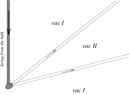
Figure 7: Two type of strings in the world-volume theory. A bulk string is a bound state of the $a$ and the $\bar{b}$ domain lines.

In the (2+1) dimensional effective theory on the wall the end-point of the bulk ANO string is seen as an electric charge coupled to the (dual) U(1) gauge field at $\beta=0$ [10, 14, 34, 35]. However, at non-vanishing $\beta$ we can no longer dualize the phase $\sigma$ into the U(1) gauge field because the cosine term in (67) becomes non-local. Therefore, at nonvanishing $\beta$ it is better to use the sine-Gordon formulation (67). In this formulation the end-point of the bulk ANO string looks as a vortex of the field $\sigma$ in the $(x,y)$-plane. At $\beta=0$ this vortex is given by the solution [10]

$$\sigma=\alpha,$$ (74)

where $\alpha$ is the polar angle in the $(x,y)$-plane. At nonvanishing $\beta$ the vortex $\sigma(\alpha)$ has two jumps — each by the angle $\pi$ — tied up to the directions of the $a$ and $\bar{b}$ domain lines. We see that at $\beta\neq 0$ we have no local description of the junction of the bulk ANO string with $a$ and $\bar{b}$ domain lines.

Now we can move the heavy trial monopole (the source of the bulk ANO string) towards the wall. The length of the bulk string becomes shorter and, eventually, when the monopole hits the wall, the bulk string disappears. The configuration becomes a junction of the monopole trapped inside the wall with the $a$ and $\bar{b}$ domain lines. It is depicted, on the $(x,y)$-plane, in Fig. 8. This construction is analogous (conceptually rather than technically) to non-Abelian strings in the bulk, whose junction represents a monopole trapped on the string [27, 15, 16, 17]. If a pair of such wall-trapped monopoles (more precisely, an $M\bar{M}$ pair) is nailed at two distant fixed points on the 2D plane, the strings stretched between them are slightly curved because of their repulsion due to their non-BPS nature.

Figure 8: A static configuration where a monopole is the junction of two domain lines is possible on the wall world-volume.

7 Conclusions

In this paper we presented an explicit construction of the domain line solitons in a weakly coupled $\mathcal{N}=2$ Abelian theory. In our example the world-volume effective theory describing physics on the wall is the sine-Gordon model in $2+1$ dimensions, with two degenerate vacua. The domain line is a kink of the sine-Gordon effective Lagrangian. Magnetic charges on the wall are confined by these objects; the magnetic flux carried by them is one half of the one carried by the the Abrikosov–Nielsen–Olesen flux tubes in the bulk.

The effective description of the world-volume physics found in this theory is different from the Chern-Simon description proposed for the domain-wall world-volume theory in $\mathcal{N}=1$ super-Yang–Mills in Ref. [24], and we know why. In particular, the Chern-Simon term is local only in terms of the dual gauge field description while, on the other hand, the sine-Gordon description is local only in terms of the phase field $\sigma$.

Also we would like to note that instantons inside domain wall in five dimensional gauge theory were recently discussed in [20]. In the effective world volume theory these instantons are seen as skyrmions. This has certain analogy with our results: string-like objects inside the domain wall are seen as kinks in the effective sine-Gordon theory on the wall.

References

- [1] N. Seiberg and E. Witten, Nucl. Phys. B426, 19 (1994), (E) B430, 485 (1994) [hep-th/9407087].
- [2] N. Seiberg and E. Witten, Nucl. Phys. B431, 484 (1994) [hep-th/9408099].
- [3] A. Hanany and D. Tong, JHEP 0307, 037 (2003) [hep-th/0306150].
- [4] R. Auzzi, S. Bolognesi, J. Evslin, K. Konishi and A. Yung, Nucl. Phys. B 673 (2003) 187 [hep-th/0307287].
- [5] G. W. Gibbons and P. K. Townsend, Phys. Rev. Lett. 83 (1999) 1727 [hep-th/9905196]; S. M. Carroll, S. Hellerman and M. Trodden, Phys. Rev. D 61 (2000) 065001 [hep-th/9905217].
- [6] A. Gorsky and M. A. Shifman, Phys. Rev. D 61, 085001 (2000) [hep-th/9909015].
- [7] M. A. Shifman and T. ter Veldhuis, Phys. Rev. D 62 (2000) 065004 [hep-th/9912162].
- [8] H. Oda, K. Ito, M. Naganuma and N. Sakai, Phys. Lett. B 471 (1999) 140 [hep-th/9910095]; K. Ito, M. Naganuma, H. Oda and N. Sakai, Nucl. Phys. B 586 (2000) 231 [hep-th/0004188]; M. Naganuma, M. Nitta and N. Sakai, Phys. Rev. D 65 (2002) 045016 [hep-th/0108179]; K. Kakimoto and N. Sakai, Phys. Rev. D 68 (2003) 065005 [hep-th/0306077].
- [9] M. Eto, Y. Isozumi, M. Nitta, K. Ohashi and N. Sakai, Phys. Rev. D 72 (2005) 085004 [hep-th/0506135]; M. Eto, Y. Isozumi, M. Nitta, K. Ohashi and N. Sakai, Phys. Lett. B 632 (2006) 384 [hep-th/0508241].
- [10] M. Shifman and A. Yung, Phys. Rev. D 67 (2003) 125007 [hep-th/0212293].
- [11] Y. Isozumi, M. Nitta, K. Ohashi and N. Sakai, Phys. Rev. D 71 (2005) 065018 [hep-th/0405129].
- [12] M. Shifman and A. Yung, Phys. Rev. D 70, 025013 (2004) [hep-th/0312257].
- [13] N. Sakai and D. Tong, JHEP 0503, 019 (2005) [hep-th/0501207].
- [14] R. Auzzi, M. Shifman and A. Yung, Phys. Rev. D 72 (2005) 025002 [hep-th/0504148].
- [15] M. Shifman and A. Yung, Phys. Rev. D 70, 045004 (2004) [hep-th/0403149].
- [16] A. Hanany and D. Tong, JHEP 0404 (2004) 066, [hep-th/0403158].
- [17] R. Auzzi, S. Bolognesi and J. Evslin, JHEP 0502, 046 (2005) [hep-th/0411074].
- [18] D. Tong, TASI Lectures on Solitons, hep-th/0509216.
- [19] M. Eto, Y. Isozumi, M. Nitta, K. Ohashi and N. Sakai, Solitons in the Higgs Phase — the Moduli Matrix Approach, hep-th/0602170.
- [20] M. Eto, M. Nitta, K. Ohashi and D. Tong, Phys. Rev. Lett. 95 (2005) 252003 [arXiv:hep-th/0508130].
- [21] A. M. Polyakov, Nucl. Phys. B 120, 429 (1977).
- [22] G. R. Dvali and M. A. Shifman, Phys. Lett. B 396, 64 (1997) (E) B407, 452 (1997), [hep-th/9612128].
- [23] A. Kovner, M. A. Shifman and A. Smilga, Phys. Rev. D 56, 7978 (1997) [hep-th/9706089].
- [24] B. S. Acharya and C. Vafa, On Domain Walls of Supersymmetric Yang–Mills in Four Dimensions, hep-th/0103011.
- [25] A. Ritz, M. Shifman and A. Vainshtein, Phys. Rev. D 66, 065015 (2002) [hep-th/0205083];
- [26] A. Ritz, M. Shifman and A. Vainshtein, Phys. Rev. D 70 (2004) 095003 [hep-th/0405175].
- [27] D. Tong, Phys. Rev. D 69 (2004) 065003, [hep-th/0307302].
- [28] V. Markov, A. Marshakov and A. Yung, Nucl. Phys. B 709, 267 (2005) [hep-th/0408235].
- [29] A. Hanany, M. J. Strassler and A. Zaffaroni, Nucl. Phys. B 513, 87 (1998) [hep-th/9707244].
- [30] A. I. Vainshtein and A. Yung, Nucl. Phys. B 614, 3 (2001) [hep-th/0012250].
- [31] J. P. Gauntlett, D. Tong and P. K. Townsend, Phys. Rev. D 63 (2001) 085001 [hep-th/0007124]; Phys. Rev. D 64 (2001) 025010 [hep-th/0012178]; J. P. Gauntlett, R. Portugues, D. Tong and P. K. Townsend, Phys. Rev. D 63 (2001) 085002 [hep-th/0008221].
- [32] M. Arai, M. Naganuma, M. Nitta and N. Sakai, Nucl. Phys. B 652 (2003) 35 [hep-th/0211103]; BPS Wall in SUSY Nonlinear Sigma Model with Eguchi-Hanson Manifold, in Garden of Quanta, Eds. J. Arafune, et al., (World Scientific, Singapore, 2003), p. 299, [hep-th/0302028].
-
[33]
A. Abrikosov, Sov. Phys. JETP 32, 1442 (1957)
[Reprinted in Solitons and Particles, Eds. C. Rebbi and G. Soliani
(World Scientific, Singapore, 1984), p. 356];
H. Nielsen and P. Olesen, Nucl. Phys. B61, 45 (1973) [Reprinted in Solitons and Particles, Eds. C. Rebbi and G. Soliani (World Scientific, Singapore, 1984), p. 365]. - [34] D. Tong, JHEP 0602, 030 (2006) [hep-th/0512192];
- [35] M. Shifman and A. Yung, Bulk-Brane Duality in Field Theory, hep-th/0603236.
- [36] E. Bogomolny, Sov. J. Nucl. Phys. 24, 449 (1976). [Reprinted in Solitons and Particles, Eds. C. Rebbi and G. Soliani (World Scientific, Singapore, 1984), p. 389].