Cosmologies from higher-order string corrections

Abstract.

We study cosmologies based on low-energy effective string theory with higher-order string corrections to a tree-level action and with a modulus scalar field (dilaton or compactification modulus). In the presence of such corrections it is possible to construct nonsingular cosmological solutions in the context of Pre-Big-Bang and Ekpyrotic universes. We review the construction of nonsingular bouncing solutions and resulting density perturbations in Pre-Big-Bang and Ekpyrotic models. We also discuss the effect of higher-order string corrections on dark energy universe and show several interesting possibilities of the avoidance of future singularities.

1. Introduction

String theory has continuously stimulated its application to cosmology in a number of profound ways [1, 2, 3]. It is actually very important to test the viability of string theory by extracting cosmological implications from it. In particular string cosmology has an exciting possibility to resolve the big-bang singularity which plagues in General Relativity.

The Pre-Big-Bang (PBB) model [4, 5] based on the low energy, tree-level string effective action is one of the first attempts to apply string theory to cosmology. In this scenario there exist two disconnected branches, one of which corresponds to the dilaton-driven inflationary stage and another of which is the Friedmann branch with a decreasing curvature. Then string corrections to the effective action can be important around the high-curvature regime where the branch change occurs. Ekpyrotic/Cyclic cosmologies [6, 7, 8] have a similarity to the PBB scenario in the sense that the description in terms of the tree-level effective action breaks down around the collision of two branes in a five dimensional bulk.

When the universe evolves toward the strongly coupled, high-curvature regime with growing dilaton, it is inevitable to implement higher-order string corrections to the tree-level action. Indeed it was found that two branches can be smoothly joined by taking into account the dilatonic higher-order string corrections in the context of PBB [9, 10] and Ekpyrotic [11] scenarios. In the system where a (compactification) modulus field is dynamically important rather than the dilaton, Antoniadis et al. showed that the big-bang singularity can be avoided by including the Gauss-Bonnet (GB) curvature invariant coupled to the modulus [12].

In order to test these string-motivated models from observations, it is important to investigate spectra of density perturbations and to compare them with temperature anisotropies in Cosmic Microwave Background (CMB). For example, inflationary cosmology generically predicts nearly scale-invariant spectra of density perturbations. This prediction agrees well with the recent observations in CMB anisotropies [13]. While inflationary cosmology is based upon the potential energy of a scalar field with a slow-roll evolution, the kinematic energy of dilaton or modulus field dominates in PBB and Ekpyrotic/Cyclic cosmologies. Hence it is expected that the spectrum of density perturbations in the latter case is different from the prediction in inflationary cosmology. We shall address the problem of density perturbations generated in PBB and Ekpyrotic/Cyclic cosmologies by using nonsingular bouncing solutions obtained by including second-order string corrections. We note that the effect of string corrections can be important in constructing inflation models, see Refs. [14] for such possibilities.

The effect of such string corrections can be also important in the context of dark energy. From recent observations the equation of state (EOS) parameter $w$ of dark energy lies in a narrow strip around $w=-1$ quite likely being below of this value [15, 16] (see Refs. [17] for reviews of dark energy). The region where the EOS parameter $w$ is less than $-1$ is referred as a phantom (ghost) dark energy universe [18]. The phantom dominated universe ends up with a finite-time future singularity called Big Rip or Cosmic Doomsday [19, 20, 21]. The Big Rip singularity is characterized by divergent behavior of the energy and curvature invariants at Big Rip time. Hence it is natural to account for higher-order curvature corrections in the presence of dark energy [22, 23, 24, 25, 26, 27, 28, 29, 30, 31, 32]. In fact it is possible to avoid or moderate the Big Rip singularity when such corrections are present [22, 24, 25] and showed that it is possible to avoid or moderate the Big Rip singularity. We shall review cosmological solutions in second-order string gravity in the context of dark energy and consider the avoidance of future singularities.

In what follows the effect of string corrections will be reviewed in two separate sections–(i) PBB/Ekpyrotic cosmologies (sec. 2) and (ii) dark energy universe (sec. 3). It is interesting to note that such corrections can play important roles for both past and future singularities.

2. Pre-Big-Bang and Ekpyrotic cosmologies

The PBB scenario is based upon low-energy, tree-level effective string theory using toroidal compactifications [4, 5]. The string effective action in four dimensions is given by

$${\cal S}_{S}\,=\,\int{\rm d}^{4}x\sqrt{-g}e^{-\phi}\left[\frac{1}{2}R+\frac{1}{2}(\nabla\phi)^{2}-V_{S}(\phi)+{\cal L}_{c}+{\cal L}_{m}\right]\,,$$ (1)

where $\phi$ is a dilaton field that controls the string coupling parameter, $g_{s}^{2}=e^{\phi}$, and $\sqrt{-g}$ is the determinant of metric $g_{\mu\nu}$. We neglect here additional modulus fields corresponding to the size and shape of the internal space of extra dimensions. The potential $V_{S}(\phi)$ for the dilaton vanishes in the perturbative string effective action. The Lagrangian ${\cal L}_{c}$ corresponds to higher-order string corrections which we will present later, whereas ${\cal L}_{m}$ is the Lagrangian of additional matter fields (e.g., fluids, kinetic components, axion etc.). In this section we do not consider the contribution of ${\cal L}_{m}$, but in Sec. 3 we will account for it as a barotropic fluid. The above action is so-called the “string frame” action in which the dilaton is coupled to a scalar curvature, $R$.

The dilaton $\phi$ starts out from a weakly coupled regime ($g_{s}\ll 1$) and evolves toward a strongly coupled region ($g_{s}>1$). The Hubble parameter grows during this stage. This “superinflation” is driven by a kinematic energy of the dilaton field, which is so-called a PBB branch. There exists another Friedmann branch with a decreasing curvature. It is possible to connect the two branches by accounting for higher-order string corrections ${\cal L}_{c}$ to the tree-level action [9, 10, 33, 34]. This is one of the main topics in this review.

In Ekpyrotic [6, 7] and Cyclic [8] cosmologies the universe contracts before the bounce because of the presence of a negative potential characterizing an attraction force between two parallel branes in an extra-dimensional bulk. The collision of two parallel branes signals the beginning of the hot, expanding, big bang of standard cosmology. After the brane collision the universe connects to a standard Friedmann branch as in the case of PBB cosmology. The origin of large-scale structure is supposed to be generated by quantum fluctuations of a field $\phi$ characterizing the separation of a bulk brane. It is important to construct nonsingular bouncing cosmological solutions in order to make concrete prediction of the power spectrum generated in Ekpyrotic/Cyclic cosmologies. This is actually possible by accounting for higher-order string corrections as in the PBB case [11].

The PBB model has a similarity to Ekpyrotic/Cyclic cosmologies in a sense that the universe exhibits a bounce in “Einstein frame”. Making a conformal transformation

$$\hat{g}_{\mu\nu}=e^{-\phi}g_{\mu\nu}\,,$$ (2)

the action in Einstein frame is given by

$${\cal S}_{E}\,=\,\int{\rm d}^{4}x\sqrt{-\hat{g}}\left[\frac{1}{2}\hat{R}-\frac{1}{4}(\hat{\nabla}\phi)^{2}-V_{E}(\phi)+\cdots\right]\,,$$ (3)

where $V_{E}(\phi)\equiv e^{\phi}V_{S}(\phi)$. Introducing a rescaled field $\varphi=\pm\phi/\sqrt{2}$, the action (3) yields

$${\cal S}_{E}\,=\,\int{\rm d}^{4}x\sqrt{-\hat{g}}\left[\frac{1}{2}\hat{R}-\frac{1}{2}(\hat{\nabla}\varphi)^{2}-V_{E}(\phi(\varphi))+\cdots\right]\,.$$ (4)

This is the action for an ordinary scalar field $\varphi$ with potential $V_{E}$. Hence it can be used to describe both the PBB model in Einstein frame, as well as the ekpyrotic scenario [35].

In the original version of the Ekpyrotic scenario [6], the Einstein frame is used where the coupling to the Ricci curvature is fixed, and the field $\phi$ describes the separation of a bulk brane from our four-dimensional orbifold fixed plane. In the case of the second version of the Ekpyrotic scenario [7] and in the cyclic scenario [8], $\phi$ is the modulus field denoting the size of the orbifold (the separation of the two orbifold fixed planes).

The Ekpyrotic scenario is described by a negative exponential potential [6]

$$V_{E}=-V_{0}\exp\left(-\sqrt{\frac{2}{p}}\,\varphi\right)\,,$$ (5)

with $0<p\ll 1$. The branes are initially widely separated but are approaching each other, which means that $\varphi$ begins near $+\infty$ and is decreasing toward $\varphi=0$. In the PBB scenario the dilaton starts to evolve from a weakly coupled regime with $\phi$ increasing from $-\infty$. If we want the potential (5) to describe a modified PBB scenario with a dilaton potential which is important when $\phi\to 0$ but negligible for $\phi\to-\infty$, we have to use the relation $\varphi=-\phi/\sqrt{2}$ between the field $\varphi$ in the ekpyrotic case and the dilaton $\phi$ in the PBB case.

In the flat Friedmann-Robertson-Walker (FRW) metric ${\rm d}s^{2}=-{\rm d}t_{E}^{2}+a_{E}^{2}{\rm d}x_{E}^{2}$ in Einstein frame, the background equations with ${\cal L}_{c}=0$ are given by

$$3H_{E}^{2}=\frac{1}{2}\dot{\varphi}^{2}+V_{E}(\varphi)\,,$$ (6)

$$\ddot{\varphi}+3H_{E}\dot{\varphi}+\frac{{\rm d}V_{E}}{{\rm d}\varphi}=0\,,$$ (7)

where a dot represents a derivative with respect to $t_{E}$ and $H_{E}\equiv\dot{a}_{E}/a_{E}$. Here the subscript “E ” denotes the quantities in the Einstein frame. The exponential potential (5) has the following exact solution [36]

$$a_{E}\propto|t_{E}|^{p},\quad H_{E}=\frac{p}{t_{E}},\quad V_{E}=-\frac{p(1-3p)}{t_{E}^{2}},\quad\dot{\varphi}=\frac{\sqrt{2p}}{t_{E}}\,.$$ (8)

The solution for $t_{E}<0$ describes the contracting universe prior to the collision of branes. The Ekpyrotic scenario corresponds to a slow contraction with $0<p\ll 1$. From Eq. (8) the potential vanishes for $p=1/3$, which corresponds to the PBB scenario.

In string frame the scale factor $a_{S}$ and the cosmic time $t_{S}$ are related with those in Einstein frame via the relation ${\rm d}t_{S}=e^{-\varphi/\sqrt{2}}{\rm d}t_{E}$ and $a_{S}=e^{-\varphi/\sqrt{2}}a_{E}$. Then we find [11, 35]

$$a_{S}\propto(-t_{S})^{-\sqrt{p}},\quad\phi=-\frac{2\sqrt{p}}{1-\sqrt{p}}\ln\left[-(1-\sqrt{p})t_{S}\right]\,.$$ (9)

This illustrates a super-inflationary solution with growing dilaton. Hence the contraction in Einstein frame corresponds to the superinflation driven by a kinematic energy of the field $\phi$. We note that there exists another branch of an accelerated contraction ($a_{S}\propto(-t_{S})^{\sqrt{p}}$) [3], but this is out of our interest.

The above solution needs to be regularized around $t_{S}=0$ (or $t_{E}=0$) in order to connect to the Friedmann branch after the bounce. In the context of PBB cosmology, it was realized that higher-order string corrections (defined in the string frame) to the action induced by inverse string tension and coupling constant corrections can yield a nonsingular background cosmology. A possible set of corrections include terms of the form [9, 10]

$${\cal L}_{c}=-\frac{1}{2}\alpha^{\prime}\lambda\zeta(\phi)\left[cR_{\rm GB}^{2}+d(\nabla\phi)^{4}\right]\,,$$ (10)

where $\alpha^{\prime}$ is a string expansion parameter, $\zeta(\phi)$ is a general function of $\phi$ and $R_{\rm GB}^{2}=R^{2}-4R^{\mu\nu}R_{\mu\nu}+R^{\alpha\beta\mu\nu}R_{\alpha\beta\mu\nu}$ is the Gauss-Bonnet (GB) term. $\lambda$ is an additional parameter which depends on the types of string theories: $\lambda=-1/4$, $-1/8$ and 0 correspond to bosonic, heterotic and superstrings, respectively. If we require that the full action agrees with the three-graviton scattering amplitude, the coefficients $c_{i}^{\prime}s$ are fixed to be $c=-1$ and $d=1$ with $\zeta(\phi)=-e^{-\phi}$ [37].

The corrections ${\cal L}_{c}$ are the sum of the tree-level $\alpha^{\prime}$ corrections and the quantum $n$-loop corrections ($n=1,2,3,\cdots$), with the function $\xi(\phi)$ given by

$$\zeta(\phi)=-\sum_{n=0}C_{n}e^{(n-1)\phi}\,,$$ (11)

where $C_{n}$ ($n\geq 1$) are coefficients of $n$-loop corrections, with $C_{0}=1$. There exist regular cosmological solutions in the presence of tree-level and one-loop corrections, but this is not realistic in the sense that the Hubble rate in Einstein frame continues to increase after the bounce (see Fig. 1 of Ref. [11]). Nonsingular bouncing solutions that connect to a Friedmann branch can be obtained by accounting for the corrections up to two-loop with a negative coefficient ($C_{2}<0$).

It was shown in Ref. [11] that nonsingular bouncing solutions exist in Einstein frame even in the presence of a negative exponential potential. When $p\ll 1$ the potential is vanishingly small for $\varphi\gg 1$, in which case the dynamics of the system is practically the same as that of the zero potential discussed in Ref. [10]. In this case the dilaton starts out from the low-curvature regime $|\phi|\gg 1$, which is followed by the string phase with linearly growing dilaton and nearly constant Hubble parameter. During the string phase one has [9]

$$a_{S}\propto(-\eta_{S})^{-1},\quad\phi=-\frac{\dot{\phi}_{f}}{H_{f}}{\rm ln}(-\eta_{S})+{\rm const}\,,$$ (12)

where $\dot{\phi}_{f}\simeq 1.40$ and $H_{f}\simeq 0.62$. In the Einstein frame this corresponds to a contracting Universe with

$$a_{E}\propto(-\eta_{E})^{\dot{\phi}_{f}/(2H_{f})-1}\,.$$ (13)

On the other hand, we can consider the scenario where the negative Ekpyrotic potential dominates initially but the higher-order correction becomes important when two branes approach sufficiently. By including the correction terms of ${\cal L}_{c}$ only for $\varphi~{}\mbox{\raisebox{-4.30554pt}{$\stackrel{{\scriptstyle\textstyle<}}{{\textstyle\sim}}$}}~{}1$, we have numerically confirmed that it is possible to obtain regular bouncing solutions, see Fig. 1. In this case the background solutions are described by Eq. (8) or (9) before the higher-order correction terms begin to work.

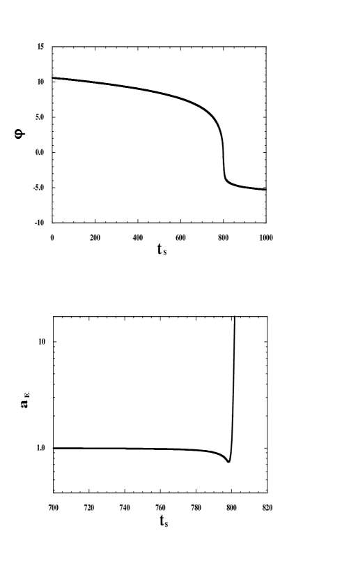
Figure 1. Evolution of $\varphi$ and $a_{E}$ with $c=-1$, $d=1$, $p=0.1$, $C_{1}=1.0$ and $C_{2}=-1.0\times 10^{-3}$. In this case we include the correction term ${\cal L}_{c}$ only for $\varphi<1$. We choose initial conditions $\phi=-15$, $H=1.5\times 10^{-3}$. Prior to the collision of branes at $\varphi=0$, the universe is slowly contracting, which is followed by the bouncing solution through higher-order corrections.

The spectrum of scalar perturbations was studied by a number of authors in the cases of PBB cosmology [38, 39, 40] and Ekpyrotic cosmology [41, 42, 43, 44] (see also Ref. [45]). A perturbed space-time metric has the following form for scalar perturbations in an arbitrary gauge [46]:

$${\rm d}s^{2}=-(1+2A){\rm d}t^{2}+2a(t)B_{,i}{\rm d}x^{i}{\rm d}t+a^{2}(t)[(1-2\psi)\delta_{ij}+2E_{,i,j}]{\rm d}x^{i}{\rm d}x^{j}\,,$$ (14)

where a comma denotes the usual flat space coordinate derivative. The curvature perturbation, ${\cal R}$, in the comoving gauge is given by [47]

$${\cal R}\equiv\psi+\frac{H}{\dot{\phi}}\delta\phi\,.$$ (15)

The power spectrum of ${\cal R}$ is defined by ${\cal P}_{\cal R}\equiv k^{3}|{\cal R}|^{2}/(2\pi^{2})\propto k^{n_{\cal R}-1}$, where $k$ is a comoving wavenumber. The spectral index $n_{\cal R}$ of curvature perturbations generated before the bounce is given by [45, 41] (see also Refs. [42, 43, 44]):

$$n_{\cal{R}}-1 = \frac{2}{1-p}\,\,\,\,\,\,\,\,\,({\rm for}~{}~{}0<p\leq 1/3)\,,$$ (16)

$$= \frac{4-6p}{1-p}\,\,\,\,\,\,\,\,\,({\rm for}~{}~{}1/3\leq p<1)\,.$$ (17)

We see that a scale-invariant spectrum with $n_{\cal R}=1$ is obtained either as $p\to\infty$ in an expanding universe, corresponding to conventional slow-roll inflation, or for $p=2/3$ during collapse [48, 45]. In the case of the PBB cosmology ($p=1/3$) one has $n_{\cal{R}}=4$, which is a highly blue-tilted spectrum. The ekpyrotic scenario corresponds to a slow contraction ($0<p\ll 1$), in which case we have $n_{\cal{R}}\simeq 3$.

The spectrum (16) corresponds to the one generated before the bounce. In order to obtain the final power spectrum at sufficient late-times in an expanding branch, we need to connect the contracting branch with the Friedmann (expanding) one. As we mentioned, the two branches are joined each other by including the corrections given in Eq. (11). This then allows the study of the evolution of cosmological perturbations without having to use matching prescriptions. The effects of the higher-order string corrections to the action on the evolution of fluctuations in the PBB cosmology was investigated numerically in [49, 11]. It was found that the final spectrum of fluctuations is highly blue-tilted ($n_{\cal R}\simeq 4$) and the result obtained is the same as what follows from the analysis using matching conditions between two Einstein Universes [50, 51] joined along a constant scalar field hypersurface.

It was shown in Ref. [11] that the spectrum of curvature perturbations long after the bounce is given as $n_{\cal R}\simeq 3$ for $0<p\ll 1$ by numerically solving perturbation equations in a nonsingular background regularized by the correction term (10). In particular comoving curvature perturbations are conserved on cosmologically relevant scales much larger than the Hubble radius around the bounce, which means that the spectrum (16) can be used in an expanding background long after the bounce.

The authors in [7] showed that the spectrum of the gravitational potential $\Phi$, generated before the bounce is nearly scale-invariant for $0<p\ll 1$, i.e., $n_{\Phi}-1=-2p/(1-p)$. A number of authors argued [41, 42, 43, 44] that this corresponds to the growing mode in the contracting phase but to the decaying mode in the expanding phase. Cartier [52] recently performed detailed numerical analysis using nonsingular perturbation equations and found that in the case of the $\alpha^{\prime}$-regularized bounce both $\Phi$ and ${\cal R}$ exhibit the highly blue-tilted spectrum (16) long after the bounce. It was numerically shown that the dominant mode of the gravitational potential is fully converted into the post-bounce decaying mode. Similar conclusions have also been reached in investigations of perturbations in other specific non-singular models [53]. Arguments can given that the comoving curvature perturbation is conserved for adiabatic perturbations on large scales under very general conditions [41, 54].

Nevertheless we have to caution that these studies are based on non-singular four-dimensional bounce models and in the Ekpyrotic/Cyclic model the bounce is only non-singular in a higher-dimensional completion of the model [55]. The ability of the ekpyrotic/cyclic model to produce a scale-invariant spectrum of curvature perturbations after the bounce relies on this higher-dimensional physics being fundamentally different from conventional four-dimensional physics, such that the growing mode of $\Phi$ in the contracting phase does not decay after the bounce [56].

3. Dark energy

In the previous section we have discussed the role of higher-order string corrections to the tree-level action in the context of early universe. Recent observations show that the present universe is dominated by dark energy responsible for an accelerated expansion. When the universe is dominated by a phantom matter ($w<-1$), this leads to the growth of the energy and curvature invariants. In such a circumstance higher-order string corrections may be important when the energy scale grows up to a Planck one. We are interested in the effect of such corrections around the Big Rip singularity. In fact the Big Rip singularity can be avoided in the presence of such corrections as we will see in this section. We shall also derive cosmological solutions for an effective string Lagrangian together with a barotropic perfect fluid.

Our starting action is the generalization of (1):

$${\cal S}=\int{\rm d}^{D}x\sqrt{-g}\left[\frac{1}{2}f(\phi,R)-\frac{1}{2}\omega(\phi)(\nabla\phi)^{2}-V(\phi)+\xi(\phi){\cal L}_{c}^{(\phi)}+{\cal L}_{m}^{(\phi)}\right]\,,$$ (18)

where $\phi$ is a scalar field corresponding either to the dilaton or to another modulus, and $f$ is a generic function of the scalar field and the Ricci scalar $R$. $\omega$, $\xi$ and $V$ are functions of $\phi$. In this section we do not consider the cosmological dynamics in the presence of the field potential $V$. ${\cal L}_{m}^{(\phi)}$ is the Lagrangian of a barotropic perfect fluid with energy density $\rho$ and pressure density $p$. We assume that the barotropic index, $w\equiv p/\rho$, is a constant. In general the fluid can be coupled to the scalar field $\phi$. The $\alpha^{\prime}$-order quantum corrections are encoded in the term

$${\cal L}_{c}^{(\phi)}=a_{1}R_{\alpha\beta\mu\nu}R^{\alpha\beta\mu\nu}+a_{2}R_{\mu\nu}R^{\mu\nu}+a_{3}R^{2}+a_{4}(\nabla\phi)^{4}\,,$$ (19)

where $a_{i}$ are coefficients depending on the string model one is considering. We are most interested in the Gauss-Bonnet parametrization ($a_{1}=a_{3}=1$, $a_{2}=-4$ and $a_{4}=-1$) discussed in the previous section, but we keep the coefficients general in deriving basic equations.

For a flat FRW background with a scale factor $a$, we obtain the Friedmann equation [49, 25]

$$d(d-1)FH^{2}=RF-f-2dH\dot{F}+2(\rho+\rho_{\phi}+\xi\rho_{c}),$$ (20)

where $d=D-1$ and

$$\rho_{\phi} = (\omega/2)\dot{\phi}^{2}+V,$$ (21)

$$\rho_{c} = 3a_{4}\dot{\phi}^{4}-d[4c_{1}\Xi H^{3}+(d-3)c_{1}H^{4}+c_{2}(2\Xi H\dot{H}+2dH^{2}\dot{H}-\dot{H}^{2}+2H\ddot{H})].$$ (22)

Here $F\equiv\partial f/\partial R$, $\Xi\equiv\dot{\xi}/\xi$, and

$$c_{1}\equiv 2a_{1}+da_{2}+d(d+1)a_{3},\,\,\,\,\,c_{2}\equiv 4a_{1}+(d+1)a_{2}+4da_{3}.$$ (23)

In four dimensions ($d=3$), the coefficients read $c_{1}=2a_{1}+3a_{2}+12a_{3}$ and $c_{2}=4(a_{1}+a_{2}+3a_{3})$, while the $H^{4}$ term in $\rho_{c}$ vanishes. At low energy it was shown that the unique higher-order gravitational Lagrangian giving a theory without ghosts is the Gauss–Bonnet one ($a_{1}=a_{3}=1$, $a_{2}=-4$, $a_{4}=-1$). In this case, $c_{2}$ vanishes identically while $c_{1}=2+d(d-3)$. With fixed dilaton coupling ($\Xi=0$) equation (20) reduces to the standard Friedmann equation in four dimensions, in agreement with the fact that the GB term is topological when $d=3$. In three dimensions ($d=2$), the GB higher-derivative contribution vanishes identically except for the $\dot{\phi}^{4}$ term.

The continuity equation for the dark energy fluid contains a source term given by the coupling between this fluid and the scalar field $\phi$. We choose the covariant coupling considered in [57]: $\delta{\cal S}_{m}/\delta\phi=-\sqrt{-g}\,Q(\phi)\rho$, where ${\cal S}_{m}=\int{\rm d}^{D}x\sqrt{-g}{\cal L}_{m}^{(\phi)}$ and $Q(\phi)$ is an unknown function which we shall set to a constant later. In synchronous gauge we have

$$\dot{\rho}+dH\rho(1+w)=Q\dot{\phi}\rho,$$ (24)

while the equation of motion for the field $\phi$ is

$$\omega(\ddot{\phi}+dH\dot{\phi})+V^{\prime}-\xi^{\prime}{\cal L}_{c}^{(\phi)}+4a_{4}\xi\dot{\phi}^{2}(3\ddot{\phi}+dH\dot{\phi}+\Xi\dot{\phi})+\left(\dot{\omega}\dot{\phi}-\omega^{\prime}\frac{\dot{\phi}^{2}}{2}-\frac{f^{\prime}}{2}\right)=-Q\rho,$$ (25)

where the Lagrangian of the quantum correction is written as

$${\cal L}_{c}^{(\phi)}=d\left[(d+1)c_{1}H^{4}+4c_{1}H^{2}\dot{H}+c_{2}\dot{H}^{2}\right]+a_{4}\dot{\phi}^{4}.$$ (26)

Equations (20)–(25) are the master equations of the physical system under study. We note that the $\dot{\phi}^{4}$ term can be important even in the absence of curvature corrections in a dilatonic ghost condensate model [59].

The massless dilaton discussed in the previous section corresponds to

$$F=-\omega=e^{-\phi},\,\,\,\,\,V=0,\,\,\,\,\,\xi=\frac{\lambda}{2}e^{-\phi}.$$ (27)

The full contribution of $n$-loop corrections is given by Eq. (11). In this work we shall take only the tree-level term (27) into account.

Generally moduli fields appear whenever a submanifold of the target spacetime is compactified with compactification radii described by the expectation values of the moduli themselves. In the case of a single modulus (one common characteristic length) and heterotic string ($\lambda=1/8$), the four-dimensional action corresponds to [58]

$$F=1,\,\,\,\,\omega=3/2,\,\,\,\,a_{4}=0,\,\,\,\,\xi=-\frac{\delta}{16}\ln[2e^{\phi}\eta^{4}(ie^{\phi})],$$ (28)

where $\eta$ is the Dedekind function and $\delta$ is a constant proportional to the 4D trace anomaly. $\delta$ depends on the number of chiral, vector, and spin-$3/2$ massless supermultiplets of the $N=2$ sector of the theory. In general it can be either positive or negative, but it is positive for the theories in which not too many vector bosons are present. Again the scalar field corresponds to a flat direction in the space of nonequivalent vacua and $V=0$. At large $\phi$ the last equation can be approximated as

$$\xi\approx\xi_{0}\cosh\phi,\,\,\,\,\,\xi_{0}\equiv\frac{\pi\delta}{24},$$ (29)

which we shall use instead of the exact expression. In fact it was shown in Ref. [60] that this approximation gives results very close to those of the exact case.

3.1. Modulus driven solution

In Ref. [25] cosmological solutions based on the action (18) without a potential ($V=0$) were discussed in details for three cases–(i) fixed scalar field ($\dot{\phi}=0$), (ii) linear dilaton ($\dot{\phi}={\rm const}$), and (iii) logarithmic modulus ($\dot{\phi}\propto 1/t$). In the case (i) we obtain geometrical inflationary solutions only for $D\neq 4$. In the case (ii) pure de-Sitter solutions exist in string frame, but this corresponds to a contracting universe in Einstein frame. These solutions are not realistic when we apply to dark energy. In what follows we shall focus on cosmological solutions in the case (iii) with a fixed dilaton.

Introducing the following new variables

$$x\equiv H\,,\qquad y\equiv\dot{H}\,,\qquad u\equiv\phi\,,\qquad v\equiv\dot{\phi}\,,\qquad z\equiv\rho\,,$$ (30)

the equations of motion for the modulus action corresponding to Eqs. (20)-(25) read

$$\dot{x}=y,$$ (31)

$$\dot{y}=\frac{2z+3v^{2}/2-d(d-1)x^{2}-8dc_{1}\dot{\xi}x^{3}-2d(d-3)c_{1}\xi x^{4}-2dc_{2}\xi y(2\Xi x+2dx^{2}-y)}{4dc_{2}\xi x},$$

(32)

$$\dot{v}=\frac{2d}{3}\xi^{\prime}[(d+1)c_{1}x^{4}+4c_{1}x^{2}y+c_{2}y^{2}]-dxv-\frac{2Q}{3}z,$$ (33)

$$\dot{z}=\left[-dx(1+w)+Qv\right]z.$$ (34)

While only derivatives of $\xi$ appear in the equations of motion for $d=3$ and $c_{2}=0$ (GB case), there are non-vanishing contributions of $\xi$ itself for general coefficients $c_{i}$. When $c_{2}=0$, the equations of motion for $x$ and $v$ read

$$\dot{x} = \frac{\dot{z}+3v\dot{v}/2-dc_{1}x^{3}[4\ddot{\xi}+(d-3)\dot{\xi}x]}{dx[(d-1)+12c_{1}\dot{\xi}x+4(d-3)c_{1}\xi x^{2}]},$$ (35)

$$\frac{\dot{v}}{v^{2}} = \frac{2d}{3}c_{1}\xi^{\prime}\frac{x^{2}}{v^{2}}[(d+1)x^{2}+4\dot{x}]-d\frac{x}{v}-\frac{2Q}{3}\frac{z}{v^{2}},$$ (36)

while the Friedmann equation is

$$d(d-1)\frac{x^{2}}{v^{2}}-\frac{3}{2}-2\frac{z}{v^{2}}+2dc_{1}\xi\frac{x^{3}}{v^{2}}[4\Xi+(d-3)x]=0.$$ (37)

In addition $c_{1}$ can be set equal to 1 and absorbed in the definition of $\xi_{0}$, so that the coefficient $c_{2}$ is the only free parameter of the higher-order Lagrangian.

We search for future asymptotic solution of the form

$$x \sim \omega_{1}t^{\beta},\quad y\sim\beta\omega_{1}t^{\beta-1},\quad u\sim u_{0}+\omega_{2}\ln t,\quad v\sim\frac{\omega_{2}}{t},\quad\xi\sim\frac{1}{2}\xi_{0}e^{u_{0}}t^{\omega_{2}},$$ (38)

$$z \sim z_{0}t^{Q\omega_{2}}\exp\left[-\frac{d(1+w)\omega_{1}}{\beta+1}t^{\beta+1}\right],\qquad\beta\neq-1,$$ (39)

$$z \sim z_{0}t^{\alpha},\qquad\beta=-1,$$ (40)

where the barotropic index $w$ is constant and

$$\alpha\equiv Q\omega_{2}-d(1+w)\omega_{1}.$$ (41)

We define $\tilde{\delta}\equiv(1/2)c_{1}\xi_{0}e^{u_{0}}$, so that in any claim involving the sign of $\tilde{\delta}$ ($\delta$) a positive $c_{1}$ coefficient is understood. In order to find a solution in the limit $t\to+\infty$, one has to match the exponents of $t$ to get algebraic equations in the parameters $\beta,\omega_{i},c_{2}$ and $\tilde{\delta}$.

In Ref. [58, 25] the following four solutions were found. We can obtain a number of analytic solutions depending on the regimes we are in:

1. A low-curvature regime in which $\xi$ terms are subdominant at late times.

2. An intermediate regime where some terms in the equations of motion, either coupled to $\xi$ or not, are damped.

3. A high-curvature regime in which $\xi$ terms dominate.

4. A solution of the form (38)–(40) for the full equations of motion.

Below we summarize the properties of each solution.

1. A low-curvature regime

   In this regime the solution is given by

   $$\beta=-1,\qquad\omega_{2}<2,$$ (42)

   with the constraints

   $$\omega_{1}=\frac{1}{d}-\frac{2Qz_{0}t^{\alpha+2}}{3d\omega_{2}},\quad 3\omega_{2}^{2}=2d(d-1)\omega_{1}^{2}-4z_{0}t^{\alpha+2},\quad\alpha\leq-2.$$ (43)

2. An intermediate regime

   In this regime the solution exists only for $c_{2}=0$ and is given by

   $$\beta=-2,\quad\omega_{2}=5,\quad Q\leq-2/5,\quad\omega_{1}^{3}=\frac{1}{16d\tilde{\delta}}\left(15-2Qz_{0}t^{5Q+2}\right),$$ (44)

   for a non-vanishing fluid. The condition, $\tilde{\delta}>0$, is required in order to obtain an expanding solution characterized by $a(t)\sim a_{0}\exp(-\omega_{1}/t)$. This solution reaches Minkowski spacetime asymptotically. If the fluid decays, then one recovers the $C_{\infty}$ solution of Ref. [58] with $d=3$ and $z=0$.

3. A high-curvature regime

   In this regime the solution is given by

   $$\beta=-1,\quad\omega_{2}>2,\quad\alpha\leq\omega_{2}-4,$$ (45)

   together with constraint equations

   $$\tilde{\delta}d\omega_{1}^{2}[(d+1)\omega_{1}^{2}-4\omega_{1}+c_{2}]-Qz_{0}t^{\alpha-\omega_{2}+4}=0,$$ (46)

   $$d\tilde{\delta}\omega_{1}^{2}[(3-d)\omega_{1}^{2}-4\omega_{2}\omega_{1}+c_{2}(2d\omega_{1}+2\omega_{2}-3)]+z_{0}t^{\alpha-\omega_{2}+4}=0.$$ (47)

   In the GB case ($c_{2}=0$) the solution corresponding to a decaying fluid ($\alpha<\omega_{2}-4$) is

   $$\omega_{1}=\frac{4}{d+1},\quad\omega_{2}=\frac{3-d}{d+1},$$ (48)

   which contradicts the condition (45) in any dimension. Hence in the GB scenario with $\omega_{2}\neq 4$ only the marginal case $\alpha=\omega_{2}-4$ is allowed.

4. An exact solution

   An exact solution which is valid at all times is

   $$\beta=-1,\quad\omega_{2}=2,$$ (49)

   together with the constraints on $\omega_{1}$:

   $$2\tilde{\delta}d\omega_{1}^{2}[(d+1)\omega_{1}^{2}-4\omega_{1}+c_{2}]-6d\omega_{1}+6-Qz_{0}t^{\alpha+2}=0,$$ (50)

   $$2\tilde{\delta}d\omega_{1}^{2}[(d-3)\omega_{1}^{2}+8\omega_{1}-c_{2}(2d\omega_{1}+1)]+d(d-1)\omega_{1}^{2}-6-2z_{0}t^{\alpha+2}=0,$$ (51)

   and Eq. (43).

The low-curvature solution (42) and the Minkowski solution (44) can be joined each other if the coupling constant $\delta$ given in Eq. (28) is negative [58, 61]. The exact solution (49) is found to be unstable in numerical simulations of Ref. [25]. In the asymptotic future the solutions tend to approach the low-curvature one given by Eq. (42) rather than the others, irrespective of the sign of the modulus-to-curvature coupling $\delta$.

3.2. Constraints from the recent universe

We compare the observational constraints on $\omega_{1}$ for the recent evolution of the universe with the modulus solutions found in the previous section ($d=3$). The situation we study is the case in which a perfect fluid is vanishing asymptotically. The results are summarized in Table 3.2 at the 68% confidence level. We also address the cases in the presence of a cosmological constant $\Lambda$. Note that the solution (44) in an intermediate regime is discarded.

[htb]

Solutions $t\to\infty$	$\omega_{1}^{(0)}$	Stability
Low curvature		Yes
High curvature, $c_{2}=0$		$\Lambda>0$
High curvature, $c_{2}\neq 0$, $\Lambda=0$
High curvature, $c_{2}\neq 0$, $\Lambda\neq 0$	$\omega_{1}^{+}$, $c_{2}<-8$	$\omega_{1}^{+}$, $\Lambda>0$
Exact, $c_{2}=0$
Exact, $c_{2}\neq 0$	Yes

Constraints on modulus solutions in the asymptotic future for the Hubble parameter $H=\omega_{1}t^{-1}$, vanishing fluid, and $d=3$. Blank entries are excluded by experiments or numerical analysis.

The logarithmic modulus solution with the GB parametrization and no extra fluid does not provide a viable cosmological evolution in the current universe. In the next subsection, however, we will see that the GB case in the presence of dark energy fluid may exhibit interesting features for the future evolution of the universe. The low redshift constraint on $c_{2}$ for the high curvature solution ($\Lambda\neq 0$) can be relaxed up to $c_{2}<-1$ at the 99% confidence level. Hence we have shown that there are models which can in principle explain the current acceleration without using the dark energy fluid.

The situation becomes more complicated in the presence of a barotropic fluid. The low-curvature solution can describe the very recent universe if $Q$ is negative and non-vanishing. The other cases crucially depend upon the interplay between all the theoretical parameters.

3.3. Dark energy universe with modulus gravity

In the universe dominated by a phantom fluid ($w<-1$), the energy density of the universe continues to grow and the Hubble rate eventually exhibits a divergence at finite time (Big Rip). Then the effect of higher-order curvature corrections can become important when the energy density grows up to the Planck scale. In fact it was shown that quantum curvature corrections coming from conformal anomaly can moderate the future singularities [63, 22].

We would like to consider the effect of $\alpha^{\prime}$ quantum corrections when the curvature of the universe increases in the presence of a phantom fluid. We shall concentrate on the modulus case with $\xi$ given by Eq. (29). Our main interest is the cosmological evolution in four dimensions ($d=3$) in the presence of a GB term. The dilaton is assumed to be fixed, so that there are no long-range forces to take into account except gravity.

From the discussion in subsection 3.1, the growth of the barotropic fluid is weaker than that of the Hubble rate when the condition

$$\alpha=Q\omega_{2}-d(1+w)\omega_{1}\leq-2\,,$$ (52)

is satisfied. This condition is not achieved for a phantom fluid when the coupling $Q$ between the fluid and the field $\phi$ is absent ($Q=0$).

Figure 2. Evolution of $H$ and $\rho$ with $\xi_{0}=-2$, $w=-1.1$ for (a) $Q=0$ and (b) $Q=-5$. We choose initial conditions as $H_{i}=0.2$, $\phi_{i}=2.0$ and $\rho_{i}=0.1$. The curves (a1) and (b1) represent the evolution of $H$ for $Q=0$ and $Q=-5$, respectively, while the curves (a2) and (b2) show the evolution of $\rho$ for corresponding $Q$.

In Ref. [25] the equations of motion were solved numerically by varying initial conditions of $H$, $\phi$ and $\rho$. When $\delta<0$, we numerically found that the solutions approach a Big Rip singularity for $Q=0$ and $w<-1$ (see Fig. 2). The condition (43) can be satisfied for negative $Q$ provided that $\omega_{2}$ is positive. In Fig. 2 we plot the evolution of $H$ and $\rho$ for $Q=-5$ and $w=-1.1$. In this case $\rho$ decreases faster than $t^{-2}$, which means that the energy density of the fluid eventually becomes negligible relative to that of the modulus. Hence the universe approaches the low-curvature solution given by Eq. (42) at late times, thereby showing the avoidance of Big Rip singularity even for $w<-1$. By substituting the asymptotic values $\omega_{1}=1/3$ and $\omega_{2}=2/3$ in equation (43), the condition for decaying fluid reads $Q<3(w-1)/2=-3.15$. We checked that the Big Rip singularity can be avoided in a wide range of the parameter space for negative $Q$. These results do not change even for smaller values of $\delta$ such as $|\delta|={\cal O}(1)$ (corresponding to $|\xi_{0}|=0.1$).

When $Q$ is positive, the condition (43) is not satisfied for $\omega_{2}>0$. However numerical calculations show that $\dot{\phi}$ becomes negative even if $\dot{\phi}>0$ initially. We found that the system approaches the low-energy regime characterized by $\omega_{1}=1/3$ and $\omega_{2}=-2/3$. Since $\omega_{2}<0$, the Big Rip singularity can be avoided even for positive $Q$. In fact we numerically checked that the Hubble rate continues to decrease provided that the condition (43) is satisfied in the asymptotic regime.

When $\delta>0$, there is another interesting situation in which the Hubble rate decreases in spite of the increase of the energy density of the fluid. This corresponds to the solution in the high-curvature regime in which the growing energy density $\rho$ can balance with the GB term ($\rho\approx 24H^{3}\dot{\xi}$ in the Friedmann equation). In this case the Big Rip does not appear even when $w<-1$ and $Q=0$. Thus the GB corrections provide us several interesting possibilities to avoid the Big Rip singularity.

3.4. Other corrections

We should mention several attempts to apply curvature corrections to dark energy. Nojiri et al. [23] studied the case of the tree-level dilatonic-type coupling (27) in the presence of an exponential potential and showed that the scalar-Gauss-Bonnet coupling acts against the occurrence of the Big Rip singularity. In Ref. [24] the evolution of phantom dark energy universe was studied with fixed dilaton and modulus by taking into account string corrections up to the 4-th order. It was found that the universe reaches a Big Crunch singularity instead of a Big Rip one for type II strings, while the Big Rip singularity is not avoided for heterotic and bosonic strings.

Apart from string corrections, a number of authors [62, 63, 22, 64, 65] studied the effect of quantum backreactions of conformal matter around several singularities which can appear in future. They usually contain second-order curvature corrections such as the Gauss-Bonnet term and the square of a Weyl tensor. In Ref. [22] it was shown that quantum corrections coming from conformal anomaly can be important when the curvature of the universe grows large, which typically moderates future singularities. Finally we note that loop quantum cosmology leads to a modified Friedmann equation when the energy scale grows to a Planck one, which typically gives us a regular cosmological evolution without future singularities [66].

4. Conclusions

In this article we have discussed cosmological implications of higher-order string corrections to the tree-level effective action. In the context of Pre-Big-Bang (PBB) and Ekpyrotic cosmologies regular bouncing solutions can be constructed by including such corrections. This allows us to evaluate the spectrum of density perturbations long after the bounce. For the correction terms given by Eq. (11) we found that the spectra of scalar perturbations are highly blue-tilted: $n_{\cal R}=4$ in the PBB case and $n_{\cal R}=3$ in the Ekpyrotic case. This is different from the nearly scale-invariant spectrum ($n_{\cal R}\simeq 1$) observed in CMB anisotropies. As long as nonsingular bouncing solutions are constructed by using the correction terms presented in this paper, we need another scalar field (e.g., curvaton [67]) to generate nearly scale-invariant density perturbations.

We also applied second-order string corrections to dark energy. In particular we reviewed several cosmological solutions in the presence of modulus-type corrections with a fixed dilaton. In the asymptotic future the solutions tend to approach the low-curvature one given by equation (42) rather than the others, irrespective of the sign of the modulus-to-curvature coupling $\delta$. We placed constraints on the viability of modulus-driven solutions using the current observational data. The Gauss-Bonnet parametrization is excluded in any of the above mentioned regimes when a barotropic fluid is vanishing; see table 3.2. In the presence of a phantom dark energy fluid we discussed the effect of the modulus coupling with Gauss-Bonnet curvature invariants. It is possible to consider a situation in which the energy density of the fluid decays when the coupling $Q$ between the field $\phi$ and the phantom fluid ($w<-1$) is present. We showed that the Big Rip singularity can be avoided for the coupling $Q$ which satisfies the condition $Q\omega_{2}-3(1+w)\omega_{1}<-2$ asymptotically. This is actually achieved irrespective of the sign of $Q$ and the asymptotic solutions are described by the low-curvature one given by Eq. (42). We also briefly mentioned the effect of other forms of higher-order string corrections to future singularities.

Thus we showed that string corrections can be important in a number of cosmological situations. We hope that the development of string theory will further provide us rich and fruitful implications to cosmology.

References

- [1] J. E. Lidsey, D. Wands and E. J. Copeland, Phys. Rept. 337, 343 (2000).
- [2] M. P. Dabrowski, Annalen Phys. 10 (2001) 195.
- [3] M. Gasperini and G. Veneziano, Phys. Rept. 373, 1 (2003).
- [4] G. Veneziano, Phys. Lett. B 265, 287 (1991); K. A. Meissner and G. Veneziano, Phys. Lett. B 267, 33 (1991).
- [5] M. Gasperini and G. Veneziano, Astropart. Phys. 1 (1993) 317.
- [6] J. Khoury, B. A. Ovrut, P. J. Steinhardt and N. Turok, Phys. Rev. D 64, 123522 (2001).
- [7] J. Khoury, B. A. Ovrut, P. J. Steinhardt and N. Turok, Phys. Rev. D 66, 046005 (2002).
- [8] P. J. Steinhardt and N. Turok, Science 296, 1436 (2002); Phys. Rev. D 65, 126003 (2002).
- [9] M. Gasperini, M. Maggiore and G. Veneziano, Nucl. Phys. B 494, 315 (1997).
- [10] R. Brustein and R. Madden, Phys. Rev. D 57, 712 (1998).
- [11] S. Tsujikawa, R. Brandenberger and F. Finelli, Phys. Rev. D 66, 083513 (2002).
- [12] I. Antoniadis, J. Rizos and K. Tamvakis, Nucl. Phys. B 415, 497 (1994).
- [13] D. N. Spergel et al., Astrophys. J. Suppl. 148, 175 (2003).
- [14] A. A. Starobinsky, Phys. Lett. B 91, 99 (1980); M. C. Bento and O. Bertolami, Phys. Lett. B 228, 348 (1989); Class. Quant. Grav. 17, 4855 (2000); S. W. Hawking, T. Hertog and H. S. Reall, Phys. Rev. D 63, 083504 (2001); K. i. Maeda and N. Ohta, Phys. Lett. B 597, 400 (2004); Phys. Rev. D 71, 063520 (2005); K. Akune, K. i. Maeda and N. Ohta, Phys. Rev. D 73, 103506 (2006).
- [15] A. G. Riess et al. [Supernova Search Team Collaboration], Astron. J. 116, 1009 (1998); S. Perlmutter et al., Astrophys. J. 517, 565 (1999); A. G. Riess et al., Astrophys. J. 607, 665 (2004).
- [16] U. Alam, V. Sahni, T. D. Saini and A. A. Starobinsky, Mon. Not. Roy. Astron. Soc. 354, 275 (2004); P. S. Corasaniti, M. Kunz, D. Parkinson, E. J. Copeland and B. A. Bassett, Phys. Rev. D 70, 083006 (2004).
- [17] V. Sahni and A. A. Starobinsky, Int. J. Mod. Phys. D 9, 373 (2000); V. Sahni, Lect. Notes Phys. 653, 141 (2004); S. M. Carroll, Living Rev. Rel. 4, 1 (2001); T. Padmanabhan, Phys. Rept. 380, 235 (2003); P. J. E. Peebles and B. Ratra, Rev. Mod. Phys. 75, 559 (2003); E. J. Copeland, M. Sami and S. Tsujikawa, arXiv:hep-th/0603057.
- [18] R. R. Caldwell, Phys. Lett. B 545, 23 (2002).
- [19] R. R. Caldwell, M. Kamionkowski and N. N. Weinberg, Phys. Rev. Lett. 91, 071301 (2003).
- [20] S. M. Carroll, M. Hoffman and M. Trodden, Phys. Rev. D 68, 023509 (2003).
- [21] P. Singh, M. Sami and N. Dadhich, Phys. Rev. D 68, 023522 (2003).
- [22] S. Nojiri, S. D. Odintsov and S. Tsujikawa, Phys. Rev. D 71, 063004 (2005).
- [23] S. Nojiri, S. D. Odintsov and M. Sasaki, Phys. Rev. D 71, 123509 (2005).
- [24] M. Sami, A. Toporensky, P. V. Tretjakov and S. Tsujikawa, Phys. Lett. B 619, 193 (2005).
- [25] G. Calcagni, S. Tsujikawa and M. Sami, Class. Quant. Grav. 22, 3977 (2005).
- [26] L. Amendola, C. Charmousis and S. C. Davis, arXiv:hep-th/0506137.
- [27] B. M. N. Carter and I. P. Neupane, arXiv:hep-th/0510109; arXiv:hep-th/0512262; I. P. Neupane, arXiv:hep-th/0602097.
- [28] G. Cognola, E. Elizalde, S. Nojiri, S. D. Odintsov and S. Zerbini, Phys. Rev. D 73, 084007 (2006).
- [29] G. Calcagni, B. de Carlos and A. De Felice, arXiv:hep-th/0604201.
- [30] I. Y. Aref’eva and A. S. Koshelev, arXiv:hep-th/0605085.
- [31] S. Nojiri, S. D. Odintsov and M. Sami, arXiv:hep-th/0605039.
- [32] T. Koivisto and D. F. Mota, arXiv:astro-ph/0606078.
- [33] S. Foffa, M. Maggiore and R. Sturani, Nucl. Phys. B 552, 395 (1999).
- [34] C. Cartier, E. J. Copeland and R. Madden, JHEP 0001, 035 (2000).
- [35] R. Durrer and F. Vernizzi, Phys. Rev. D 66, 083503 (2002).
- [36] F. Lucchin and S. Matarrese, Phys. Rev. D 32, 1316 (1985).
- [37] R. R. Metsaev and A. A. Tseytlin, Nucl. Phys. B 293, 385 (1987).
- [38] R. Brustein, M. Gasperini, M. Giovannini, V. F. Mukhanov and G. Veneziano, Phys. Rev. D 51, 6744 (1995).
- [39] E. J. Copeland, R. Easther and D. Wands, Phys. Rev. D 56, 874 (1997).
- [40] J. c. Hwang, Astropart. Phys. 8, 201 (1998).
- [41] D. H. Lyth, Phys. Lett. B 524, 1 (2002); Phys. Lett. B 526, 173 (2002).
- [42] R. Brandenberger and F. Finelli, JHEP 0111, 056 (2001).
- [43] J. c. Hwang, Phys. Rev. D 65, 063514 (2002).
- [44] S. Tsujikawa, Phys. Lett. B 526, 179 (2002).
- [45] D. Wands, Phys. Rev. D 60, 023507 (1999).
- [46] H. Kodama and M. Sasaki, Prog. Theor. Phys. Suppl. 78, 1 (1984); V. F. Mukhanov, H. A. Feldman and R. H. Brandenberger, Phys. Rept. 215, 203 (1992); B. A. Bassett, S. Tsujikawa and D. Wands, Rev. Mod. Phys. 78, 537 (2006).
- [47] D. H. Lyth, Phys. Rev. D 31, 1792 (1985).
- [48] A. A. Starobinsky, JETP Lett. 30 (1979) 682 [Pisma Zh. Eksp. Teor. Fiz. 30 (1979) 719].
- [49] C. Cartier, J. c. Hwang and E. J. Copeland, Phys. Rev. D 64, 103504 (2001).
- [50] R. Brustein, M. Gasperini, M. Giovannini, V. F. Mukhanov and G. Veneziano, Phys. Rev. D 51, 6744 (1995).
- [51] N. Deruelle and V. F. Mukhanov, Phys. Rev. D 52, 5549 (1995).
- [52] C. Cartier, arXiv:hep-th/0401036.
- [53] M. Gasperini, M. Giovannini and G. Veneziano, Phys. Lett. B 569, 113 (2003); M. Gasperini, M. Giovannini and G. Veneziano, Nucl. Phys. B 694, 206 (2004); L. E. Allen and D. Wands, Phys. Rev. D 70, 063515 (2004); T. J. Battefeld and G. Geshnizjani, Phys. Rev. D 73, 064013 (2006); V. Bozza and G. Veneziano, JCAP 0509, 007 (2005); V. Bozza, JCAP 0602, 009 (2006); M. Giovannini, Phys. Rev. D 73, 083505 (2006).
- [54] P. Creminelli, A. Nicolis and M. Zaldarriaga, Phys. Rev. D 71, 063505 (2005).
- [55] A. J. Tolley and N. Turok, Phys. Rev. D 66, 106005 (2002).
- [56] A. J. Tolley, N. Turok and P. J. Steinhardt, Phys. Rev. D 69, 106005 (2004).
- [57] L. Amendola, Phys. Rev. D 60, 043501 (1999); Phys. Rev. D 62, 043511 (2000); B. Gumjudpai, T. Naskar, M. Sami and S. Tsujikawa, JCAP 0506, 007 (2005); L. Amendola, M. Quartin, S. Tsujikawa and I. Waga, Phys. Rev. D 74, 023525 (2006).
- [58] I. Antoniadis, J. Rizos and K. Tamvakis, Nucl. Phys. B 415, 497 (1994).
- [59] F. Piazza and S. Tsujikawa, JCAP 0407, 004 (2004).
- [60] H. Yajima, K. i. Maeda and H. Ohkubo, Phys. Rev. D 62, 024020 (2000); A. Toporensky and S. Tsujikawa, Phys. Rev. D 65, 123509 (2002).
- [61] P. Kanti, J. Rizos and K. Tamvakis, Phys. Rev. D 59, 083512 (1999).
- [62] E. Elizalde, S. Nojiri and S. D. Odintsov, Phys. Rev. D 70, 043539 (2004).
- [63] S. Nojiri and S. D. Odintsov, Phys. Lett. B 595, 1 (2004); Phys. Rev. D 70, 103522 (2004).
- [64] S. K. Srivastava, arXiv:hep-th/0411221.
- [65] P. Tretyakov, A. Toporensky, Y. Shtanov and V. Sahni, Class. Quant. Grav. 23, 3259 (2006).
- [66] M. Sami, P. Singh and S. Tsujikawa, arXiv:gr-qc/0605113, Physical Review D to appear.
- [67] D. H. Lyth and D. Wands, Phys. Lett. B 524, 5 (2002); K. Enqvist and M. S. Sloth, Nucl. Phys. B 626, 395 (2002); T. Moroi and T. Takahashi, Phys. Lett. B 522, 215 (2001) [Erratum-ibid. B 539, 303 (2002)].