We consider the Renormalization-Group coupled equations for the effective potential $V(\phi)$ and the field strength $Z(\phi)$ in the spontaneously broken phase as a function of the infrared cutoff momentum $k$. In the $k\to 0$ limit, the numerical solution of the coupled equations, while consistent with the expected convexity property of $V(\phi)$, indicates a sharp peaking of $Z(\phi)$ close to the end points of the flatness region that define the physical realization of the broken phase. This might represent further evidence in favor of the non-trivial vacuum field renormalization effect already discovered with variational methods.

Pacs 11.10.Hi , 11.10.Kk

1.  Renormalization Group (RG) techniques originally inspired to the Kadanoff-Wilson blocking procedure [1] represent a powerful method to approach non-perturbative phenomena in quantum field theory. A widely accepted technique consists in starting from a bare action defined at some ultraviolet cutoff $\Lambda$ and effectively integrating out shells of quantum modes down to an infrared cutoff $k$. This procedure provides a $k-$dependent effective action $\Gamma_{k}[\Phi]$ that evolves into the full effective action $\Gamma[\Phi]$ in the limit $k\to 0$.

The $k-$dependence of $\Gamma_{k}[\Phi]$ is determined by a differential functional flow equation that is known in the literature in slightly different forms [2, 3, 4, 5, 6]. In particular, with the flows discussed in detail in Ref.[7] one starts form first principles and obtains a class of functionals that interpolates between the classical bare Euclidean action and the full effective action of the theory. However, some features, such as the basic convexity property of the effective action for $k\to 0$ [8, 9, 10, 11], are independent of the particular approach.

In this Letter, we shall study the coupled equations for the $k-$dependent effective potential $V_{k}(\phi)$ and field strength $Z_{k}(\phi)$, which naturally appear in a derivative expansion of $\Gamma_{k}[\Phi]$ (around the coordinate independent configuration $\Phi(x)=\phi$ ), using a proper-time infrared regulator. This approach generates evolution equations which are well defined truncations of the first-principle flows within a background field formulation [12, 13]. Incidentally, as shown in [12], they are also an approxmation to another exact flow (a generalised Callan-Symanzik flow) without background fields.

The equations for $V_{k}(\phi)$ and $Z_{k}(\phi)$, derived in Ref.[14], correspond to such first-principle flows up to additional terms explicitly determined in Ref.[12]. An indication of the reliability of such an approximation is provided by the consistent computation of the critical exponents in scalar self-interacting theories for various numbers $D$ of the space-time dimensions and $N$ of field components [14]. At the same time, in Ref.[11], it was shown that going beyond the approximation $Z=1$ is essential to reproduce successfully the energy gap between the exact ground state and the first excited state of the double well potential in the quantum-mechanical limit of the theory $D=1$. In addition, the coupled equations obtained by using the proper time regulator are not affected by singularities and/or ambiguities that instead appear using a sharp infrared cutoff [15].

With these premises, assuming the possibility to neglect the additional terms of Ref.[12] and adopting the same notations of Refs.[11, 14], we shall start our analysis considering the two equations

$$k{{\partial V}\over{\partial k}}=\left({k^{2}\over{4\pi}}\right)^{D/2}e^{-V^{\prime\prime}/(Zk^{2})}$$ (1)

$$k{{\partial Z}\over{\partial k}}=\left({k^{2}\over{4\pi}}\right)^{D/2}e^{-V^{\prime\prime}/(Zk^{2})}$$

$$\times\Biggl{(}-{{Z^{\prime\prime}}\over{Zk^{2}}}+{{(4+18D-D^{2})(Z^{\prime})^{2}}\over{24Z^{2}k^{2}}}+{{(10-D)Z^{\prime}V^{\prime\prime\prime}}\over{6(Zk^{2})^{2}}}-{{Z(V^{\prime\prime\prime})^{2}}\over{6(Zk^{2})^{3}}}\Biggr{)}$$ (2)

where we have set $V=V_{k}(\phi)$, $Z=Z_{k}(\phi)$ and used the notation $V^{\prime},Z^{\prime}$,…to indicate differentiation with respect to $\phi$. In the following, we shall first analyze these two equations to understand the approach to convexity and obtain informations on $Z$ and finally provide a possible physical interpretation of our numerical results.

2.  For a numerical solution of Eqs.(1) and (2) it is convenient to use dimensionless variables defined as follows: $t={\rm ln}(\Lambda/k)$, $x=k^{1-D/2}\phi$, $V(t,x)=k^{-D}V_{k}(\phi)$ and $Z(t,x)=Z_{k}(\phi)$. By defining the first derivative of the effective potential $f(x,t)=\partial_{x}V(t,x)$, Eqs.(1,2) become

$${{\partial f}\over{\partial t}}={{(D+2)}\over{2}}f+{{(2-D)}\over{2}}~{}x{{\partial f}\over{\partial x}}-{{1}\over{(4\pi)^{D/2}}}~{}{{\partial}\over{\partial x}}e^{-f^{\prime}/Z}$$ (3)

$${{\partial Z}\over{\partial t}} = {{(2-D)}\over{2}}~{}x{{\partial Z}\over{\partial x}}+{{1}\over{(4\pi)^{D/2}}}~{}{{\partial}\over{\partial x}}\left({{Z^{\prime}}\over{Z}}e^{-f^{\prime}/Z}\right)$$

$$-{{e^{-f^{\prime}/Z}}\over{(4\pi)^{D/2}}}~{} \Biggl{(} {{f^{\prime}(Z^{\prime})^{2}}\over{Z^{3}}}+{{18D-D^{2}-20}\over{24}}{{(Z^{\prime})^{2}}\over{Z^{2}}}+{{(4-D)Z^{\prime}f^{\prime\prime}}\over{6Z^{2}}}-{{(f^{\prime\prime})^{2}}\over{6Z^{2}}}\Biggr{)}$$ (4)

It is easy to show that these two coupled equations can be transformed into the structure ($i,j$=1-3)

$$P_{ij}{{\partial U_{j}}\over{\partial t}}+Q_{i}={{\partial R_{i}}\over{\partial x}}$$ (5)

where the components of the vector $U_{i}(x,t)$ are the unknown functions of the problem and where $P_{ij}$, $Q_{i}$ and $R_{i}$ can depend on $x,t,U_{i},{{\partial U_{i}}\over{\partial x}}$.

In this way, the numerical solution has been obtained with the help of the NAG routines that integrate a system of non-linear parabolic partial differential equations in the $(x,t)$ two-dimensional plane. The spatial discretisation is performed using a Chebyshev $C^{o}$ collocation method, and the method of lines is employed to reduce the problem to a system of ordinary differential equations. The routines contain two main parameters (the size of the discretisation grid $N_{\rm points}$ in the spatial dimension and the local accuracy $\Delta$ in the time integration) that can be changed to control the stability of the solution. In our case, after reaching sufficiently large values of $N_{\rm points}$ ($\sim 2000$) and sufficiently small values of $\Delta$ ($\sim 10^{-7}$), the numerical results remain remarkably stable for further variations of these parameters.

We shall focus on the quantum-field theoretical case $D=4$ assuming standard boundary conditions at the cutoff scale : i) a renormalizable form for the bare, broken-phase potential

$$V_{\Lambda}(\phi)=-{{1}\over{2}}M^{2}\phi^{2}+\lambda\phi^{4}$$ (6)

and ii) a unit renormalization condition for the derivative term in the bare action

$$Z_{\Lambda}(\phi)=1$$ (7)

With this choice of the classical potential the problem is manifestly invariant under the interchange $\phi\to-\phi$ at all values of $k$.

We shall also concentrate on the weak coupling limit $\lambda=0.1$, fixing $M=1$ and $\Lambda=10$. In this way, one gets a well defined hierarchy of scales where the infrared region corresponds to the limit $k\ll M\ll\Lambda$.

Before addressing the full problem, we have considered the standard approximation of setting $Z=1$. In this case, we can find a good approximation to the exact solution of Eq.(3) for large $x$ and large $t$ as a cubic polynomial with $t-$dependent coefficients

$$f_{\rm asy}(x,t)=A(t)x^{3}+B(t)x^{2}+C(t)x+D(t)$$ (8)

This type of form, motivated by RG arguments, see e.g. [16], becomes exact where $f^{\prime}$ is large and positive so that $e^{-f^{\prime}}\to 0$ yielding $A(t)=A_{0}$, $B(t)=B_{0}\exp(t)$, $C(t)=C_{0}\exp(2t)$, $D(t)=D_{0}\exp(3t)$. Higher powers $x^{n}$, with $n>3$, might also be inserted but they are suppressed by exponential terms $e^{-(n-3)t}$. At the same time, $f=0$ is also a solution of Eq.(3) and corresponds to a flat effective potential in $x$. As we shall see, the $k-$evolution, for $k\to 0$, turns out to be a sort of way to interpolate between $f=0$ and the asymptotic trend in Eq.(8).

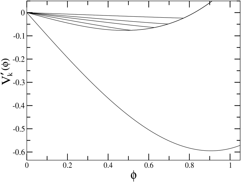
Figure 1: ${V^{\prime}}_{k}(\phi)$ vs. $\phi$, with $Z=1$ fixed, at various values of the infrared cutoff $k$: the lowest curve is for $k=\Lambda=10$, and then, from bottom to the top, $k=0.3,~{}0.13,~{}0.1,~{}0.08,~{}0.05$.

We show in Fig.1 the plots of $V^{\prime}_{k}(\phi)\equiv{{\partial V_{k}(\phi)}\over{\partial\phi}}$ at various values of the infrared cutoff down to the smallest value $k=0.05$ that can be numerically handled by our integration routine. This corresponds to a maximal value $t_{\rm max}\sim 5.3$ which is comparable to the highest value $t=5$ reported in Fig.1a of Ref.[9]. In our problem, this seems to mark the boundary of the region that is very difficult to handle numerically.

As one can see, the approach to convexity is very clean, in full agreement with the general theoretical arguments of Ref.[9]. It is characterized by an almost linear behaviour in the inner $\phi-$region that matches with the outer, asymptotic cubic shape discussed above. In this sense, the limitation in the maximal $t$ is just a numerical artifact of our integration method since from the physical point of view there should be no conceptual problem in the limit $t\to\infty$. This is supported by a fit to the slope $S(k)$ of $V^{\prime}_{k}(\phi)$ at $\phi=0$ in Fig.1, which suggests the following functional form ($a$ and $b$ being numerical coefficients obtained from the fit)

$$S(k)\sim a[{\rm exp}(-bk^{2})-1]$$ (9)

that vanishes in the limit $k\to 0$.

For small $k$, the minimum of the first derivative of the effective potential $\phi=\hat{\phi}(k)$ does not correspond to an analytic behaviour. This is a well known result of quantum field theory [17]: the Legendre-transformed effective potential is not an infinitely differentiable function.

Let us now consider the full problem defined by Eqs.(3) and (S0.Ex2). Again, for large $x$ and $t$, the pair $f=f_{\rm asy}(x,t)$ and $Z=1$ provide a simultaneous solution. However, for finite values of $k$, where the potential is not yet convex downward and $f^{\prime}<0$, the term $e^{{{|f^{\prime}|}\over{Z}}}$ drives $Z$ to grow.

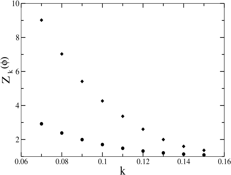
Figure 3: $Z_{k}(\phi)$ at the origin $\phi=0$ (circles) and at the peak $\phi=\hat{\phi}$ (diamonds), at different values of the infrared cutoff $k$.

We show in Fig.2, the simultaneous solutions for $Z_{k}(\phi)$ (upper panel) and $V^{\prime}_{k}(\phi)\equiv{{\partial V_{k}(\phi)}\over{\partial\phi}}$ (lower panel) for various values of the infrared cutoff down to $k=0.07$ (again $t_{\rm max}\sim 5$) that represents, for the coupled problem, the point beyond which the integration routines no longer work. The strong peaking in $Z_{k}(\phi)$, to a very high accuracy, occurs at $\hat{\phi}(k)$ where $V^{\prime}_{k}(\phi)$ has its minimum. On the basis of the general convexification property this point tends, for $k\to 0$, to the end point $\hat{\phi}(0)\equiv\phi_{0}$ of the flatness region that defines the physical realization of the broken phase. Finally, we report in Fig.3 the values of $Z_{k}(\phi)$ at $\phi=0$ (circles) and at the peak for $\phi=\hat{\phi}(k)$ (diamonds) in the range $0.07\leq k\leq 0.15$. Using some extrapolation forms, the value of the peak seems to tend, in the limit $k\to 0$, to a very large but finite value $Z_{k=0}(\phi_{0})$.

3. Let us now explore a possible physical interpretation of the numerical results reported above. We start by observing that spontaneous symmetry breaking is usually considered a semi-classical phenomenon, i.e. based on a classical potential with perturbative quantum corrections. These, with our choice of the bare parameters $\lambda=0.1$ and $M=1$ in Eq.(6), and our cutoff value $\Lambda=10$, are typically small for all quantities. In particular $Z$, in perturbation theory, is a non-leading quantity since its one-loop correction is ultraviolet finite. Therefore, the deviations from unity are expected to be very small.

Re-writing the $\Phi^{4}$ term in the standard form ${{\lambda_{\rm st}}\over{4!}}\Phi^{4}$, with $\lambda_{\rm st}=2.4$, the perturbative prediction is

$$Z_{\rm pert}-1={\cal O}({{\lambda_{\rm st}}\over{16\pi^{2}}})\sim 10^{-2}$$ (10)

This is also consistent with the assumed exact ”triviality” property of the theory for $D=4$ [18] that requires $Z\to 1$ in the continuum limit $\Lambda\to\infty$.

Now, let us compare this prediction with our $Z_{k}(\phi)$ in Fig.2. For large values of the infrared cutoff, when the effective potential is still smooth, we find $Z_{k}(\phi)\sim 1$ for all values of $\phi$, as expected. However, at smaller $k$, say $k<\delta$ with $\delta\sim 0.15$, there are large deviations from unity in the region of $\phi$ where the smooth form of the perturbative potential evolves into the typical non-analytical behaviour of the exact effective potential. This leads to the observed strong peaking phenomenon at the point $\hat{\phi}(k)$, where $V^{\prime}_{k}(\phi)$ reaches its minimum value. This point, on the basis of the general convexification property of $V(\phi)$ tends, for $k\to 0$, to the value $\hat{\phi}(0)=\phi_{0}$, the end point of the flatness region that defines the physical realization of the broken phase.

If we express the full scalar field $\Phi(x)$ as

$$\Phi(x)=\phi+h(x)$$ (11)

the above results indicate that the higher frequency components of the fluctuation field $h(x)$, those with 4-momentum $p_{\mu}$ such that $\delta\leq|p|\leq\Lambda$, represent genuine quantum corrections for all values of the background field $\phi$ in agreement with their perturbative representation as weakly coupled massive states.

On the other hand, the components with a 4-momentum $p_{\mu}$ such that $|p|\leq\delta$, are non-perturbative for values of the background field in the range $0\leq\phi\leq\hat{\phi}(|p|)$. In particular, the very low-frequency modes with $|p|\to 0$ behave non-perturbatively for all values of the background in the full range $0\leq\phi\leq\phi_{0}$. They can be thought as collective excitations of the scalar condensate and cannot be represented as standard massive states.

The existence of a peculiar $p_{\mu}\to 0$ limit in the broken phase, for which one can give some general arguments [19], finds support in the results of lattice simulations of the broken-symmetry phase (see Ref.[20]). There, differently from what happens in the symmetric phase, the connected scalar propagator deviates significantly from (the lattice version of) the massive single-particle form $1/(p^{2}+{\rm const})$ for $p_{\mu}\to 0$. In particular, looking at Figs. 7, 8 and 9 of Ref.[21], one can clearly see that, approaching the continuum limit of the lattice theory, these deviations become more and more pronounced but also confined to a smaller and smaller region of momenta near $p_{\mu}=0$.

This observation suggests that the existence of a non-perturbative infrared sector in a region $0\leq|p|\leq\delta$ might not be in contradiction with the assumed exact ”triviality” property of the theory if, in the continuum limit, the infrared scale $\delta$ vanishes in units of the physical parameter $m$ associated with the massive part of the spectrum. This means to establish a hierarchy of scales $\delta\ll m\ll\Lambda$ such that ${{\delta}\over{m}}\to 0$ when ${{m}\over{\Lambda}}\to 0$.

If this happens, the region $0\leq|p|\leq\delta$ would just shrink to the zero-measure set $p_{\mu}=0$, for the continuum theory where $m$ sets the unit mass scale, thus recovering the exact Lorentz covariance of the energy spectrum since the point $p_{\mu}=0$ forms a Lorentz-invariant subset. In this limit, the RG function $Z_{k}(\phi)$ would become a step function which is unity for all finite values of $k$ (and $\phi$) and is only singular for $k=0$ in the range $0\leq\phi\leq\phi_{0}$. In this way, one is left with a massive, free-field theory for all non-zero values of the momentum, and the only remnant of the non-trivial infrared sector is the singular re-scaling of $\phi$ (the projection of the full scalar field $\Phi(x)$ onto $p_{\mu}=0$).

This is precisely the scenario of Refs.[22], where for $\Lambda\to\infty$ the re-scaling of the scalar condensate diverges logarithmically as $\sim\ln\Lambda$ and the re-scaling of the finite-momentum modes tends to unity. The existence of such a divergent re-scaling factor for the vacuum field would have potentially important phenomenological implications for the scalar sector of the standard model and for the validity of the generally accepted upper bounds on the Higgs boson mass [22].

Of course, for a more precise comparison with the numerical results obtained in this Letter, one should study the value of the peak in $Z_{k}(\phi)$ at different values of the bare parameters to check the predicted logarithmic behaviour $Z_{\rm peak}\sim\ln(\Lambda)$ that, at the present, is just a conjecture suggested by previous works. In turn, this requires to improve on the present integration routines to extend the solution of the RG equations towards the point $k=0$ thus reducing the arbitrariness associated with different extrapolation forms.

At the same time, the existence of a peak in $Z_{k}(\phi)$ is an interesting feature that would deserve to go beyond the present numerical analysis. In this respect, since, according to [23], $V_{k}(\phi)$, for $k\to 0$, is only weakly dependent on the type of infrared regulator, we expect the peak of Z to be a physical phenomenon and not an artifact of the regulator. This can be checked by re-considering the problem from scratch at the level of the exact flow equations.

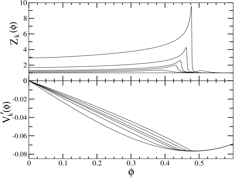
Figure 2: $Z_{k}(\phi)$ (upper panel) and ${V^{\prime}}_{k}(\phi)$ (lower panel), vs. $\phi$ at $k=$0.3, 0.15, 0.13, 0.12, 0.1, 0.07, from bottom to the top.

References

- [1] L.P. Kadanoff, Physica 2 (1966) 263; K.G. Wilson and J. Kogut, Phys. Rep. 12 (1974) 75.
- [2] F. J. Wegner and A. Houghton, Phys. Rev A8 (1973) 401.
- [3] T.S. Chang, D. D. Vvedensky and J.F. Nicoll, Phys. Rep. 217 (1992) 280.
- [4] J. Polchinski, Nucl. Phys. B 231 (1984) 269.
- [5] C. Wetterich, Nucl. Phys. B352 (1991) 529; Phys Lett. B301 (1993) 90.
- [6] T. Morris, Int. J. Mod. Phys. A 9 (1994) 2411; Phys. Lett. B329 (1994) 241.
- [7] J. Berges, N. Tetradis and C. Wetterich, Phys.Rep 363 (2002) 223.
- [8] K.-I. Aoki, A. Horikoshi, M. Taniguchi and H. Terao, The Exact Renormalization Group, Proceedings of the Workshop on the Exact Renormalization Group, Faro, Portugal, September 10-12 1998, (World Scientific 1999), arXiv:hep-th/9812050; A. S. Kapoyannis and N. Tetradis, Phys. Lett. A 276 (2000) 225.
- [9] D. F. Litim, J. M. Pawlowski and L. Vergara, Convexity of the effective action from functional flows , arXiv:hep-th/0602140.
- [10] J. Alexandre, V. Branchina and J. Polonyi, Phys. Lett. 445 (1999) 351.
- [11] D. Zappalà, Phys. Lett. A290 (2001) 35.
- [12] D.F. Litim and J. M. Pawlowski, Phys. Lett. B546 (2002) 279; Phys. Rev. D66 (2002) 025030.
- [13] D.F. Litim and J. M. Pawlowski, Phys. Lett. B516 (2001) 197; Phys. Rev. D65 (2002) 081701.
- [14] A. Bonanno and D. Zappalà, Phys. Lett. B504 (2001) 181; M.Mazza and D. Zappalà, Phys. Rev. D64 (2001) 105013.
- [15] A. Bonanno and D. Zappalà, Phys. Rev. D57 (1998) 7383; A. Bonanno, V. Branchina, H. Mohrbach and D. Zappalà, Phys. Rev. D60 (1999) 065009.
- [16] D. F. Litim, JHEP 0507 (2005) 005.
- [17] K. Symanzik, Commun. Math. Phys. 16 (1970) 48.
- [18] For a review of the rigorous results, see R. Fernández, J. Fröhlich, and A. D. Sokal, Random Walks, Critical Phenomena and Triviality in Quantum Field Theory (Springer-Verlag Berlin Heidelberg 1992).
- [19] M. Consoli, Phys. Rev. D65 (2002) 105217.
- [20] P. Cea, M. Consoli, L. Cosmai and P. M. Stevenson, Mod. Phys. Lett. A14 (1999) 1673, hep-lat/9902020.
- [21] P. M. Stevenson, Nucl. Phys. B729 [FS] (2005) 542.
- [22] M. Consoli and P.M. Stevenson, Z. Phys. C63 (1994) 427; Phys. Lett. B391 (1997) 144; Int. J. Mod. Phys. A15 (2000) 133.
- [23] A. Bonanno, G. Lacagnina, Nucl.Phys. B693 (2004) 36.