Braneworld Stars and Black Holes

Abstract:

We look for spherically symmetric star or black hole solutions on a Randall-Sundrum brane from the perspective of the bulk. We take a known bulk solution, and analyse possible braneworld trajectories within it that correspond, from the braneworld point of view, to solutions of the brane Tolman-Oppenheimer-Volkoff equations. Our solutions are therefore embedded consistently into a full bulk solution. We find the full set of static gravitating matter sources on a brane in a range of bulk spacetimes, analyzing which can correspond to physically sensible sources. Finally, we look at time-dependent trajectories in a Schwarzschild–anti de Sitter spacetime as possible descriptions of time-dependent braneworld black holes, highlighting some of the general features one might expect, as well as some of the difficulties involved in getting a full solution to the question.

1 Introduction / Motivation

The idea that spacetime may not be simply four-dimensional, but have extra dimensions as yet undetected by experiment, has become essentially accepted as fact over the past two decades, largely as a consequence of string or M-theory, but also as a result of earlier work on supergravity. Over the past few years, a new alternative has emerged in our understanding of how extra dimensions can be compactified – braneworlds and warped compactifications. Rather than the old Kaluza-Klein (KK) idea of wrapping up extra dimensions so small we only see them through extra massless fields, the braneworld idea allows us to have relatively large extra dimensions, possibly even up to the microscale, with standard particle physics confined to the “brane” and thereby unable to detect the extra dimensions at ordinary energy scales [1, 2, 3]. Gravity however can sample these extra dimensions, and one of the most alluring aspects of warped compactifications is the possibility of unusual gravitational phenomenology not only at small scales (akin to the KK picture) but at large scales, too [4, 5, 6].

The braneworld paradigm views our universe as a slice of some higher dimensional spacetime, in which we have standard four-dimensional physics confined to the brane, and only gravity (plus possibly a small number of other fields) propagating in the bulk. Confinement to the brane, while at first sounding counter-intuitive, is in fact a common occurrence. The first braneworld scenarios [1] used topological defects to model the braneworld, and zero-modes on the defects to produce confinement, and in string theory, D-branes have ‘confined’ gauge theories on their worldvolumes. The new phenomenology of braneworld scenarios is then primarily located in the gravitational sector, with a particularly nice possible resolution of the hierarchy problem being its primary motivation. Clearly however, the scenario has far outgrown these initial particle phenomenology motivations, and has proved a fertile testbed for new possibilities in cosmology, astrophysics, and quantum gravity. One of the most popular models to explore, and the one which we will be using, has been the Randall-Sundrum scenario, [3], which consists of a domain wall universe living in five-dimensional anti-de Sitter (adS) spacetime. This model can be loosely motivated by the Horava-Witten compactification of M-theory [7], and many of the ideas tested and developed in this simple, calculationally explicit model underly more recent string theory motivated compactifications [8].

The Randall-Sundrum model has one (or two) domain walls situated as minimal submanifolds in adS spacetime. In its usual form, the metric of the braneworld is

$$ds^{2}=e^{-2k|z|}\left[-dt^{2}+d{\bf x}^{2}\right]+dz^{2}\,.$$ (1)

Here, the spacetime is constructed so that there are four-dimensional flat slices stacked along the fifth $z$-dimension, which have a $z$-dependent conformal pre-factor known as the warp factor. Since this warp factor has a cusp at $z=0$, this indicates the presence of a domain wall – the braneworld – which represents an exactly flat Minkowski universe. The reason for choosing this particular slicing of adS spacetime was to have a flat Minkowski metric on the brane – i.e. to choose the “standard vacuum”.

Randall and Sundrum showed that although gravity was inherently five-dimensional, and the spacetime was strongly warped, as far as a four-dimensional brane-world observer was concerned, the gravitational potential of a particle on the brane was the Newtonian $1/r$ potential to leading order. A complete analysis shows that the graviton propagator has the correct tensor structure, and that the effect of the KK modes is to introduce a $1/r^{3}$ correction to the gravitational potential [9].

In astrophysics and cosmology we are not so much interested in the perturbative graviton propagator as in issues such as cosmological models or black holes, which are questions of non-perturbative, or strong gravity. The braneworld generalization of the FRW universe has been well explored and understood [10]; the high degree of symmetry present renders the full five-dimensional problem fully integrable [11], and the general cosmological braneworld is fully understood in terms of a slice of a five-dimensional adS black hole [12]. The mass of this bulk black hole then generates a radiation-style source for the Friedman equation. Interestingly, this understanding feeds in to the second question: What is the metric of a braneworld black hole?

At first sight it might seem that this question should be very similar to answer; as both reduce to a two-dimensional problem, however, the symmetry groups of the two spacetimes are crucially different. For cosmology, the metric splits into two parts – the two dimensions on which it depends, and the spatial part of the universe, which has constant curvature. This problem is equivalent to a two-dimensional field theory which turns out to be totally integrable. For the black hole however, the metric splits into three parts – the two dimensions on which it depends, the time coordinate and the remaining spatial part in which the horizon resides. Thus there are two fields in the two-dimensional theory, and there is no longer a simple solution [13].

The first attempt, [14], to find a black hole solution replaced the Minkowski metric in (1) by the Schwarzschild metric, thus creating a black string sticking out of the brane. Unfortunately, as suspected by the authors, this string is unstable to classical linear perturbations [15]. Chamblin et. al. realised that the true static localised black hole would actually be a slice of a five-dimensional accelerating black hole metric (known as the C-metric, [16], in four dimensions), however no such metric has as yet been found. A lower dimensional version of a black hole living on a $2+1$-dimensional braneworld was however presented by Emparan, Horowitz and Myers [17], using this four-dimensional C-metric. Since then, several authors have attempted to find the full metric using numerical techniques [18], although the main drawback seems to be that it is a very sensitive numerical system. Nonetheless, the results of [19] for small black holes are encouraging.

Analytically, progress has mostly (though see [20]) been limited to considering the brane metric equations of motion, with the only bulk input coming from the projection of the Weyl tensor, the “Weyl term” [21], onto the brane. Since this system contains an unknown bulk dependent term, assumptions have to be made either in the form of the metric or the Weyl term [22, 23]. There is no clear consensus on what the brane black hole metric is, however, some interesting features which do occur are wormholes and singular horizons [24, 23].

One of the reasons this braneworld black hole metric is so interesting is that it is believed to correspond to a quantum corrected black hole. In string theory, it has been realized for some time that there is a correspondence between string theory on adS space, and a CFT on the boundary of that adS space [25]. In other words, all of the information contained in the five-dimensional gravitational spacetime is encoded in a pure quantum field theory living on a four-dimensional spacetime. In the braneworld picture, the brane is not at the adS boundary, but at a finite distance, and the theory on this brane now contains gravity, as well as a conformal energy-momentum tensor – the Weyl term. The effect of the brane on the adS/CFT correspondence therefore is that the bulk theory of gravity in five dimensions corresponds to the four dimensional brane theory of a CFT, with a UV cutoff, interacting with gravity [26]. Since the brane theory is a quantum theory, the holographic correspondence suggests that the classical bulk solution projects to a quantum corrected solution on the brane [27]. Indeed, it was this type of argument that led Tanaka [28] to argue that the braneworld black hole metric would be time-dependent, corresponding to the back-reaction of Hawking radiation on the black hole metric.

For cosmological solutions, this holographic interpretation works very well; the presence of a black hole horizon in the bulk (which is the only allowed class of bulk solution [11]) induces a corresponding source in the Friedman equation which has the form of a radiation source. This source can be interpreted as a CFT in a thermal state corresponding to the Hawking temperature of the bulk black hole. The brane cosmological metric has a constant curvature spatial part, and its symmetries demand that only a radiation energy Weyl term is allowed. From the bulk perspective, this means that every point on the brane is at the same distance from the bulk black hole. Thus a flat universe corresponds to a ‘flat’ bulk black hole, a closed universe to a conventional spherical bulk black hole.

Transporting this intuition over to the brane black hole situation, one can imagine that the black hole becomes displaced from the “center of gravity” of the spherical wall, causing an anisotropy in the brane Weyl term, ${\cal E}_{\mu\nu}$. As the black hole gets closer to the brane, this anisotropy increases, possibly becoming more important than the radiation term. This reasoning argues for a near-horizon equation of state for ${\cal E}_{\mu\nu}$ which leads to a singular ‘event horizon’ [23], which possibly corresponds to a Boulware choice of vacuum in the quantum corrected black hole [27].

However, there is another holographic interpretation possible, and one which is far more intriguing and experimentally relevant – one which incorporates black hole evaporation. Instead of imagining a quasi-static transport of the bulk black hole towards the brane, consider a bulk geodesic. From the point of view of the brane, these trajectories have constant acceleration away from the brane, so a particle in the bulk moving along a geodesic initially moves towards the brane, can touch the brane, but then moves back into the bulk accelerating away (see section 5). Thus a black hole would move towards the brane, hit the brane, then recoil away back off to infinity. From the brane point of view, this would correspond to collapse of conformal matter, localized around the lightcone, formation of an horizon, and subsequent evaporation of the black hole, again localized around the lightcone. This picture was indeed obtained in perturbation theory in [29], where the metric of a particle leaving the brane was obtained to leading order.

Such a picture should be a reasonable approximation for small mass black holes, which, coincidentally, are precisely the type of black holes that are believed to be important in LHC and cosmic ray phenomenology (for some early works, see [30, 31]; for a more complete list of references, see [32]). Such small black holes are thought to be produced after brane-localized particles scatter at high energies and undergo gravitational collapse. A horizon is then formed engulfing the two particles, which can never escape their mutual gravitational attraction. Due to their small mass, these black holes quickly evaporate through the emission of Hawking radiation [32]: for a black hole with mass $M_{BH}\simeq 5$ TeV, and fundamental gravity scale $M_{*}=1$ TeV, their lifetime is only $\tau_{BH}\simeq 10^{-26}$ sec, and therefore exist on our brane only momentarily. Even for a higher mass, that would result in a longer lifetime, the corresponding black hole may still ‘disappear’ from our brane due to the so-called recoil effect [33, 34, 35]. Due to the absence of an analytic solution describing a black hole localized on a brane with a non-vanishing self-energy, all studies of the evaporation of brane-world black holes have been restricted to the case where the black hole mass is assumed to be significantly larger than the brane self-energy. In addition, by assuming that the black hole horizon is much smaller than the inverse adS radius, the bulk warping has also been ignored. As a result, all studies up to now have failed to consider the complete bulk-brane-black-hole gravitational system.

In the present work, we study the aforementioned gravitational system in full. Our analysis will be complementary to work on probe branes [36], and develops the work on specific brane trajectories in black hole backgrounds [37, 38]. We restrict our study to the case of a 5-dimensional spacetime in which a 3-brane with a non-negligible energy-momentum tensor is embedded. By using the Israel’s junction conditions [39], we derive a set of equations corresponding to a spherically symmetric brane with additional matter content corresponding to a homogeneous and isotropic fluid, in other words the brane equivalent of the Tolman-Oppenheimer-Volkoff (TOV) equations. The main difference between this work and the brane based work of [22] is that we have not only a complete brane solution to the TOV equations, but also the full bulk solution. In other words a genuine brane star. Clearly the general brane-bulk system has infinitely many degrees of freedom, so our approach here is to restrict to a spherically symmetric bulk solution, and a variety of bulk backgrounds are considered with the final objective being the consistent embedding of a 3-brane into a Schwarzschild–anti de Sitter spacetime.

The outline of the paper is as follows: In the next section we derive the brane equations of motion for a brane with a general isotropic fluid source living in a (general) spherically symmetric bulk. We then consider the static system in section 3, and show how the static brane is completely integrable. In section 4 we specialize to the physically relevant case of a Schwarzschild–anti de Sitter bulk, exploring possible black hole and stellar solutions. We then briefly consider time dependent solutions in section 5 before concluding.

2 The general brane equations

We now adopt a spherically-symmetric coordinate system, and write the 5-dimensional line-element in the form

$$ds^{2} = -U(r)\,d\tau^{2}+\frac{1}{U(r)}\,dr^{2}+r^{2}(d\chi^{2}+\sin^{2}\chi\,d\Omega_{{}_{\rm{II}}}^{2})\,,$$ (2)

where $U(r)$ is a general function of the global radial coordinate and $d\Omega_{{}_{\rm{II}}}^{2}$ the line element on a unit 2-sphere. We are considering configurations within the second Randall-Sundrum model with a single brane of positive tension and with spacetime reflection symmetric in the wall.

The location of the brane in the 5-dimensional bulk is described by the function $\chi(\tau,r)$. If we take a 5-vector to be described by the component functions $x^{\mu}=(\tau,r,\chi,\theta,\phi)$, we may form a new basis in terms of the (unnormalised) tangent vectors and the unit normal:

$$T^{\mu} = (1,0,\dot{\chi},0,0)$$

$$R^{\mu} = (0,1,\chi^{\prime},0,0)$$

$$\Theta^{\mu} = (0,0,0,1,0)$$ (3)

$$\Phi^{\mu} = (0,0,0,0,1)$$

$$n_{\mu} = n(-\dot{\chi},-\chi^{\prime},1,0,0)\,.$$

In the above, overdot and prime denote partial differentiation with respect to $\tau$ and $r$, respectively, and $\frac{1}{n^{2}}=\left(-\frac{\dot{\chi}^{2}}{U}+U{\chi^{\prime}}^{2}+\frac{1}{r^{2}}\right)$. The tensor $h_{\mu\nu}=g_{\mu\nu}-n_{\mu}n_{\nu}$ projects vectors onto the wall, and its tangential components define the induced metric on the brane. In the aforementioned basis, it can be simply evaluated as

$$h_{\mu\nu}=\left(\begin{array}[]{ccccc}-U+r^{2}\dot{\chi}^{2}&r^{2}\dot{\chi}\chi^{\prime}&&&\\ r^{2}\dot{\chi}\chi^{\prime}&\frac{1}{U}+r^{2}{\chi^{\prime}}^{2}&&&\\ &&r^{2}\sin^{2}\chi&&\\ &&&r^{2}\sin^{2}\chi\sin^{2}\theta&\\ &&&&0\\ \end{array}\right)\,.$$

The Israel junction conditions [39], triggered by the presence of the brane with a non-vanishing distributional energy-momentum tensor $T_{\mu\nu}$, take the form

$$\left[K_{\mu\nu}-Kh_{\mu\nu}\right]^{+}_{-}=\kappa_{5}T_{\mu\nu}\,,$$ (4)

where $K_{\mu\nu}=h^{\rho}_{\mu}h^{\sigma}_{\nu}\nabla_{\rho}n_{\sigma}$ is the extrinsic curvature of the brane, and $\kappa_{5}=8\pi G_{5}$. Using the $Z_{2}$ reflection symmetry around the wall, the Israel conditions can be rewritten as

$$K_{\mu\nu}=\frac{\kappa_{5}}{6}\left(3T_{\mu\nu}-h_{\mu\nu}\,T\right)\,.$$ (5)

Deviating from the simplified ansatz of [14] in which the brane was characterized only by a constant self-energy, in this work we assume that the energy-momentum tensor on the brane may take the general form

$$T_{\mu\nu}=\left[\rho(\tau,r)+p(\tau,r)\right]h_{\mu\sigma}h_{\nu\rho}\,u^{\sigma}u^{\rho}+p(\tau,r)\,h_{\mu\nu}\,.$$ (6)

The above ansatz describes an isotropic distribution of a perfect fluid with $\rho(\tau,r)$ and $p(\tau,r)$ the energy density and pressure, respectively, of the fluid. The vector $u^{\mu}$ is the fluid’s 4-velocity, that satisfies the normalization condition $u^{\mu}u^{\nu}h_{\mu\nu}=-1$. It can be easily shown that working in the rest frame of the fluid on the brane, i.e. writing

$$u^{\mu}=\frac{1}{\sqrt{-h_{TT}}}\,(1,0,0,0,0)$$ (7)

in the basis ($T,R,\Theta,\Phi,n$), is equivalent to taking $u^{\mu}$ to be parallel to the time-like tangent vector $T^{\mu}$ in the original basis ($\tau,r,\chi,\theta,\phi$). The ansatz (7) allows us to rewrite the brane energy-momentum tensor as:

$$T_{\mu\nu}=-(\rho+p)\,\frac{h_{\mu T}h_{\nu T}}{h_{TT}}+p\,h_{\mu\nu}\,.$$ (8)

For convenience, we will write the energy density and pressure of the perfect fluid on the brane in terms of an “equation of state” $p(\tau,r)=w(\tau,r)\rho(\tau,r)$, and define for later convenience the quantity

$$v(\tau,r)\equiv 2+3w(\tau,r)\,.$$ (9)

Note however, that unlike a standard equation of state, in which the pressure is a fixed multiple of the energy, this redefinition does not restrict the pressure in any way since $v$ is an arbitrary function of both $r$ and $\tau$.

By using the form of the energy momentum tensor given in (8) together with (9), the Israel conditions for a brane containing a perfect fluid take the form

$$K_{\mu\nu}=\frac{\kappa_{5}}{6}\,\rho\left[h_{\mu\nu}-(1+v)\,\frac{h_{\mu T}h_{\nu T}}{h_{TT}}\right],$$ (10)

or, more explicitly,

$$K_{TT}=-n\left(\ddot{\chi}+Ur\chi^{\prime}\dot{\chi}^{2}-\frac{1}{2}\,UU^{\prime}\chi^{\prime}\right)=-\frac{\kappa_{5}}{6}\,\rho v\left(-U+r^{2}\dot{\chi}^{2}\right)$$ (11)

$$K_{RR}=-n\left(\chi^{\prime\prime}+\frac{2\chi^{\prime}}{r}+\frac{U^{\prime}\chi^{\prime}}{2U}+Ur{\chi^{\prime}}^{3}\right)=\frac{\kappa_{5}}{6}\rho\left[\frac{1}{U}+r^{2}{\chi^{\prime}}^{2}+\frac{(1+v)\,r^{4}\dot{\chi}^{2}{\chi^{\prime}}^{2}}{U-r^{2}\dot{\chi}^{2}}\right]$$ (12)

$$K_{TR}=-n\left(\dot{\chi}^{\prime}+\frac{\dot{\chi}}{r}+Ur{\chi^{\prime}}^{2}\dot{\chi}-\frac{U^{\prime}\dot{\chi}}{2U}\right)=-\frac{\kappa_{5}}{6}\,\rho vr^{2}\dot{\chi}\chi^{\prime}$$ (13)

$$K_{\Theta\Theta}=-n\left(Ur\chi^{\prime}\sin^{2}\chi-\sin\chi\cos\chi\right)=\frac{\kappa_{5}}{6}\,\rho r^{2}\sin^{2}\chi\,.$$ (14)

Two additional, but not independent, equations are obtained from conservation of energy-momentum:

$$\dot{\chi}\left(1+\frac{1}{2}U^{\prime}r-U+\frac{\kappa_{5}\rho}{6n}(1+v)r^{2}\cot\chi\right) = -\frac{\kappa_{5}\dot{\rho}}{6n}r^{2}\,,$$ (15)

$$\chi^{\prime}\left(1+\frac{1}{2}U^{\prime}r-U+\frac{\kappa_{5}\rho}{6n}\,(1+v)\frac{r^{4}\dot{\chi}^{2}\cot\chi}{-U+r^{2}\dot{\chi}^{2}}\right) = -\frac{\kappa_{5}\rho^{\prime}}{6n}r^{2}\,.$$ (16)

We may summarise the above results by saying that a 4-dimensional brane containing a perfect fluid, described by its energy density $\rho(\tau,r)$ and equation of state $p(\tau,r)=w(\tau,r)\rho(\tau,r)$, can be successfully embedded in a 5-dimensional spherically-symmetric background defined by a single function $U(r)$ as long as we can find a consistent set of functions $\rho(\tau,r)$, $w(\tau,r)$ and $\chi(\tau,r)$ – with the latter denoting the position of the brane in the 5-dimensional spacetime – satisfying (11)-(16). This task is simplified if we define a new function $\alpha=r\cos\chi$, in terms of which equations (11)-(16) may be written as

$$\frac{r^{2}\ddot{\alpha}}{U}-(\alpha^{\prime}r-\alpha)\left(\frac{U^{\prime}r}{2}-U\right)+\alpha+$$

$$\hskip 99.58464pt\frac{(1+v)}{U}\left[U(\alpha^{\prime}r-\alpha)+\alpha\right]\left(-U+\frac{r^{2}{\dot{\alpha}}^{2}}{r^{2}-\alpha^{2}}\right)=0\,,$$

$$Ur^{2}\alpha^{\prime\prime}+(\alpha^{\prime}r-\alpha)\left(\frac{U^{\prime}r}{2}-U\right)-\alpha+$$

$$\hskip 79.6678pt(1+v)\frac{\left[U(\alpha^{\prime}r-\alpha)+\alpha\right]Ur^{2}{\dot{\alpha}}^{2}(\alpha^{\prime}r-\alpha)^{2}}{(r^{2}-\alpha^{2})\left(r^{2}{\dot{\alpha}}^{2}-U({r^{2}-\alpha^{2}})\right)}=0\,,$$ (18)

$$\hskip 51.21504ptr\dot{\alpha}^{\prime}-\frac{1}{2}\frac{U^{\prime}r}{U}\dot{\alpha}+(1+v)(U(\alpha^{\prime}r-\alpha)+\alpha)\frac{\dot{\alpha}(\alpha^{\prime}r-\alpha)}{(r^{2}-\alpha^{2})}=0\,,$$ (19)

$$\hskip 48.36958ptU(\alpha^{\prime}r-\alpha)+\alpha=\frac{\kappa_{5}}{6}\rho r\left(-\frac{r^{2}{\dot{\alpha}}^{2}}{U}+U(\alpha^{\prime}r-\alpha)^{2}+r^{2}-\alpha^{2}\right)^{\frac{1}{2}},$$ (20)

$$\hskip 116.65646pt\frac{\dot{\rho}r}{\rho}=r\dot{\alpha}\left(\frac{1+\frac{1}{2}U^{\prime}r-U}{U(\alpha^{\prime}r-\alpha)+\alpha}+(1+v)\frac{\alpha}{r^{2}-\alpha^{2}}\right),$$ (21)

$$\frac{\rho^{\prime}r}{\rho}=(\alpha^{\prime}r-\alpha)\left(\frac{1+\frac{U^{\prime}r}{2}-U}{U(\alpha^{\prime}r-\alpha)+\alpha}+\frac{(1+v)}{(r^{2}-\alpha^{2})}\frac{r^{2}{\dot{\alpha}}^{2}\alpha}{\left(r^{2}{\dot{\alpha}}^{2}-U({r^{2}-\alpha^{2}})\right)}\right).$$ (22)

In the above, we have also used equation (14) to eliminate the quantity $\kappa_{5}\rho/6n$ from all other equations. The above system may lead to either static or time-dependent brane configurations depending on whether time-dependence is permitted in the brane trajectory $\chi$.

2.1 The Static Brane : An exact solution

If we assume that the brane trajectory is time-independent, then considerable simplifications occur. Since $\dot{\chi}=\dot{\alpha}=0$, ${\dot{\rho}}=0$ from (21). The remaining equations (apart from (19) which is trivially satisfied) become:

$$v = -(\alpha^{\prime}r-\alpha)\left(\frac{\frac{1}{2}U^{\prime}r}{U(\alpha^{\prime}r-\alpha)+\alpha}\right),$$ (23)

$$Ur^{2}\alpha^{\prime\prime} + (\alpha^{\prime}r-\alpha)\left(\frac{1}{2}U^{\prime}r-U\right)-\alpha=0,$$ (24)

$$U(\alpha^{\prime}r-\alpha)+\alpha = \frac{\kappa_{5}}{6}\rho r\left[U(\alpha^{\prime}r-\alpha)^{2}+r^{2}-\alpha^{2}\right]^{\frac{1}{2}},$$ (25)

$$\frac{\rho^{\prime}r}{\rho} = (\alpha^{\prime}r-\alpha)\left(\frac{1+\frac{1}{2}U^{\prime}r-U}{U(\alpha^{\prime}r-\alpha)+\alpha}\right).$$ (26)

Integrating (26) gives the energy density as:

$$\rho(r)=\frac{\rho_{0}}{r^{2}}\,\left[U(\alpha^{\prime}r-\alpha)+\alpha\right],$$ (27)

where $\rho_{0}$ is an integration constant. Substituting for $\rho(r)$ in (25) yields

$$U(\alpha^{\prime}r-\alpha)^{2}-\alpha^{2}+\left(1-\frac{36}{\kappa_{5}^{2}\rho_{0}^{2}}\right)r^{2}=0\,.$$ (28)

In fact, equations (24) and (28) for $\alpha(r)$ can be integrated out in terms of a modified radial variable

$${\tilde{r}}=\int\frac{dr}{r\sqrt{U}}$$ (29)

giving:

$$\cos\chi=ae^{\tilde{r}}+be^{-\tilde{r}}\,,$$ (30)

where

$$4ab=1-\frac{36}{\kappa_{5}^{2}\rho_{0}^{2}}\,.$$ (31)

The energy density and pressure can then be straightforwardly obtained as

$$\rho=\frac{\rho_{0}}{r}\left[\sqrt{U}\left(ae^{\tilde{r}}-be^{-\tilde{r}}\right)+ae^{\tilde{r}}+be^{-\tilde{r}}\right]\,,$$ (32)

$$p(r)=-\frac{2}{3}\rho(r)-\frac{\rho_{0}U^{\prime}}{6\sqrt{U}}\left(ae^{\tilde{r}}-be^{-\tilde{r}}\right)\,.$$ (33)

Finally, we can read off the induced metric on the brane as

$$ds^{2}=-Ud\tau^{2}+\frac{36}{\kappa_{5}^{2}\rho_{0}^{2}}\,\frac{r^{2}dr^{2}}{U(r^{2}-\alpha^{2})}+(r^{2}-\alpha^{2})\,d\Omega_{{}_{\rm II}}^{2}\,.$$ (34)

Note that the constants $a$ and $b$ encode the same information as the integration constant $\rho_{0}$, and the arbitrary constant corresponding to the zero point of $\tilde{r}$ from the integration in (29).

3 Static Braneworld “Stars”

In the previous section, we showed how the static brane equations admitted an (implicit) exact solution in terms of the radial variable $\tilde{r}$, which depended on an integral of the bulk Newtonian potential $U(r)$. Although this is an exact solution, the actual properties of the brane depend on the specifics of the relation between $\tilde{r}$ and $r$. Once this is determined, we have a solution describing a static, spherically symmetric distribution of an isotropic perfect fluid on the brane, i.e. a solution to the brane TOV system. Of course, not all the trajectories we will find will have the interpretation of a star, and, to this end, a careful examination of the energy density and pressure profile will be undertaken.

As a warm up to considering more physically relevant bulk spacetimes, let us consider the simplest possible bulk – the vacuum: $U=1$. In this case ${\tilde{r}}=\ln r$, and $\alpha(r)=ar^{2}+b$. Introducing the polar coordinates

$$x^{*}=r\cos\chi\,,\;\;\;\;y^{*}=r\sin\chi\,,$$ (35)

brings the brane trajectories in the form

$$\left(x^{*}-\frac{1}{2a}\right)^{2}+y^{*2}=\frac{1}{4a^{2}}-\frac{b}{a}\,,$$ (36)

with $x^{*}=b$ in the particular case $a=0$. These solutions are of limited physical importance as they have constant energy and pressure : $\rho=2a\rho_{0}$, $p=-2\rho/3$. They correspond to an Einstein static universe,

$$ds^{2}=-d\tau^{2}+R_{0}^{2}d\Omega_{\rm III}^{2}$$ (37)

where $R_{0}^{2}=(1-4ab)/4a^{2}$.

Now let us consider a more general family of bulk spacetimes. If we make the choice $U(r)=1+Cr^{n}$ for the bulk metric function, where $C$ and $n$ are arbitrary constants, we can integrate $\tilde{r}$ straightforwardly to obtain an analytic solution

$${\tilde{r}}=\frac{1}{n}\ln\left|\frac{\sqrt{U}-1}{\sqrt{U}+1}\right|\,,$$ (38)

which allows us to write $\alpha$ in the general form:

$$\alpha(r)=\left[A\left|\sqrt{U}-1\right|^{\frac{2}{n}}+B\left(\sqrt{U}+1\right)^{\frac{2}{n}}\right]\,,$$ (39)

with $A$ and $B$ convenient redefinitions of the integration constants $a$ and $b$ appearing in the general solution (30).

These solutions (39), in conjunction with the choice for the bulk metric function $U(r)=1+Cr^{n}$, describe different brane configurations in a variety of spherically symmetric bulk backgrounds. Two such backgrounds of immediate physical significance correspond to $n=\pm 2$, i.e. pure adS spacetime, and the Schwarzschild solution in five dimensions.

3.1 A 5-dimensional Anti-de Sitter Bulk

In the case of a 5-dimensional bulk filled with a negative cosmological constant, the bulk metric function may be written as $U(r)=1+k^{2}r^{2}$, where $k$ is the inverse adS radius. The shape of the brane, $\alpha(r)$, is then given by the expression:

$$\alpha(r)\equiv r\cos\chi(r)=A\left(\sqrt{U}-1\right)+B\left(\sqrt{U}+1\right)\,,$$ (40)

where, in terms of (30), we have set ${\tilde{r}}=0$ at infinity, and $A=a/k$, and $B=b/k$. Using the polar coordinates (35), the above trajectory may be written as

$$\left(1-\beta\right)\left(x^{*}+\frac{(A-B)}{1-\beta}\right)^{2}-\beta y^{*2}=\frac{(A+B)^{2}\,\left(1-4ABk^{2}\right)}{\left(1-\beta\right)}\,,$$ (41)

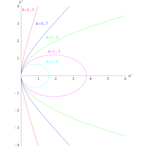
Figure 1: A selection of branes of varying coefficient $A$, for the case $B=0,k=1$ in a 5-dimensional anti-de Sitter bulk.

where $\beta=k^{2}(A+B)^{2}$. These brane trajectories can be seen to be conic sections classified by the parameter $\beta$. For $\beta>1$, the brane is an ellipsoid, $\beta=1$, a paraboloid, and for $\beta<1$ a hyperboloid, with $\beta=0$ corresponding to a straight line. In figure 1, we display the resulting brane configurations for some indicative values of the integration parameters $A$ and $B$. For simplicity, we have set $k=1$, and $B=0$; then, as $A$ varies, the shape of the brane changes gradually covering all three cases outlined above.

The physical significance of $\beta$ becomes apparent from the computation of the energy density from (27):

$$\rho=k^{2}\rho_{0}(A-B)=\frac{6k}{\kappa_{5}}\frac{k(A-B)}{\sqrt{1-\beta+k^{2}(A-B)^{2}}}\;.$$ (42)

This reveals that the energy density is constant throughout the brane, and, for $A>B$, it remains positive. Then, for the critical value $\beta=1$, the energy density has precisely the Randall-Sundrum critical value $\rho_{RS}=6k/\kappa_{5}$, while for $\beta$ less (greater) than unity we have a sub- (super-) critical brane. Turning to the equation of state on the brane, by using equations (23) and (9), we find that

$$p(r)=-\rho+\frac{(A+B)k^{2}\rho_{0}}{3\sqrt{U}}\,.$$ (43)

It is worth noting that we cannot get a static trajectory for a critical or super-critical brane with a pure tension energy momentum ($w=-1$): such a solution follows only for $A+B=0$, that corresponds to $\beta=0$ and thus to a sub-critical, or Karch-Randall brane [40]. For $\beta\neq 0$, we have a varying tension on our brane, equivalent to a surplus pressure in the braneworld.

Finally, we can evaluate the induced metric on the brane:

$$ds^{2} = -U(r)\,d\tau^{2}+\left(\frac{1-4ABk^{2}}{r^{2}-\alpha^{2}(r)}\right)\frac{r^{2}dr^{2}}{U(r)}+\left(r^{2}-\alpha^{2}(r)\right)d\Omega_{\rm{}_{II}}^{2}\,,$$ (44)

$$= -U\left(r({\hat{r}})\right)\,d\tau^{2}+\frac{d{\hat{r}}^{2}}{1-\lambda{\hat{r}}^{2}/3}+{\hat{r}}^{2}d\Omega_{\rm{}_{II}}^{2}\,.$$

where $\lambda/3=-k^{2}+\rho^{2}\kappa^{2}_{5}/36$ is the effective cosmological constant on the brane. Clearly, the spatial part of the metric takes the form of a constant curvature space, being flat, anti de Sitter or de Sitter depending on whether the brane is critical, sub- or super-critical respectively. However, since the relation between $r$ and $\hat{r}$ is in general convoluted, the brane has a nontrivial Newtonian potential. This is because unless $A=-B$, there is a nonvanishing excess pressure on the brane, which acts as a source and results in a non-asymptotically flat (or (a)dS) spacetime. To see this explicitly consider a critical brane

$$ds_{c}^{2}=-\frac{k^{2}\left(A^{2}+B^{2}+{\hat{r}}^{2}/2\right)^{2}}{(A-B)^{2}}\,d\tau^{2}+d{\hat{r}}^{2}+{\hat{r}}^{2}\,d\Omega_{\rm{}_{II}}^{2}\,.$$ (45)

This spacetime is clearly not asymptotically flat, and in fact corresponds to a source

$$T^{0}_{0}=0\,,\qquad T^{r}_{r}=T^{\theta}_{\theta}=T^{\varphi}_{\varphi}=\frac{4}{\kappa_{5}(2A^{2}+2B^{2}+\hat{r}^{2})}\,,$$ (46)

which corresponds to the actual pressure discrepancy on the brane: $p+6k/\kappa_{5}$. Similar results hold also for the case of a sub- or super-critical brane where $T^{0}_{0}=\lambda\neq 0$.

We see therefore that these particular trajectories have excess pressure on the brane, which results in metrics which do not asymptote exact Randall-Sundrum or Karch-Randall branes. However, if $|kA|$ and $|kB|$ are large enough, the metric can be flat (or asymptotically (a)dS) over many orders of magnitude before the effect of the pressure kicks in.

3.2 A 5-dimensional Schwarzschild Bulk

We now assume that the 5-dimensional bulk contains not a cosmological constant, but a mass that creates a spherically symmetric Schwarzschild background with $U(r)=1-\mu/r^{2}$, where $\mu$ is related to the actual mass of the black hole by $M=3\pi\mu/8G_{5}$. In this case, $n=-2$ and $C=-\mu$. Then, equation (39), that describes the shape of the brane, takes the form

$$\alpha(r)=r^{2}\left[A\left(\sqrt{U}-1\right)+B\left(\sqrt{U}+1\right)\right],$$ (47)

where now $A=-b/\sqrt{\mu}$, $B=a/\sqrt{\mu}$, and ${\tilde{r}}=0$ at the horizon. Note that by construction, these trajectories are strictly only valid outside the event horizon of the black hole, since the definition of the ${\tilde{r}}$ coordinate involves a branch cut there. We could in principle redefine ${\tilde{r}}$ inside the horizon, although as we are only interested in the exterior solution we shall not do so here.

Following the same analysis as before, the functions $\rho$ and $p$ are now found to be

$$\rho(r)=\rho_{0}\left[B(\sqrt{U}+1)^{2}-A(\sqrt{U}-1)^{2}\right]\;,$$ (48)

$$p(r)=-\rho(r)+\frac{\rho_{0}}{3\sqrt{U}}\left[B(\sqrt{U}+1)^{2}(2\sqrt{U}-1)-A(\sqrt{U}-1)^{2}(2\sqrt{U}+1)\right]\;,$$ (49)

where $\rho_{0}=\frac{6}{\kappa_{5}\sqrt{1+4AB\mu}}$. Clearly $\rho$ is not a constant for these branes, in contrast to the adS case, and we must now consider what we think of as a physically sensible brane energy and trajectory. Obviously we want $\rho$ to be positive, but in addition, if our solutions are to correspond to stars or black holes, we expect that they will have the interpretation of energy sources, in other words, the energy of the brane will increase towards the centre of the brane. This is not quite as straightforward as having $\rho$ be a decreasing function of $r$, since the brane radial coordinate is in fact $r\sin\chi$, and we must therefore examine each trajectory in turn.

To examine the shape of the brane, we square equation (47) to obtain:

$$4AB\,r^{2}+2(B-A)r\cos\chi-\cos\chi^{2}=\mu(A+B)^{2}\,.$$ (50)

The solutions of the above equation are hyperbolae in the $(\cos\chi,r)$-plane, which leads to the following parametric solution in polar coordinates:

$$r = \sqrt{\mu}\cosh\lambda$$ (51)

$$\chi = {\rm Arccos}\sqrt{\mu}(Be^{\lambda}-Ae^{-\lambda})\,.$$ (52)

Clearly there are constraints on the range of the parameter $\lambda$, since we require that $|\cos\chi|\leq 1$, and in addition we will impose positivity of $\rho$.

With these constraints in mind, we can see qualitatively the different families of trajectories that are allowed. First of all, note that the brane can only touch the event horizon if

$$0<B-A\leq 1/\sqrt{\mu}\,,$$ (53)

the first inequality coming from positivity of energy. Then, computing the derivative $\frac{d\chi}{dr}$ from (51, 52) shows that unless $B=-A$, $\frac{d\chi}{dr}\to\infty$ at the horizon, meaning that the brane touches the horizon at a tangent. However, if $B=-A$, then the brane can actually pass through the horizon, and, as we will see, eventually hits the central singularity.

From (50), we see that the general shape of the trajectories is in fact primarily determined by the quantity $AB$. We will now run through the general brane shapes that are allowed.

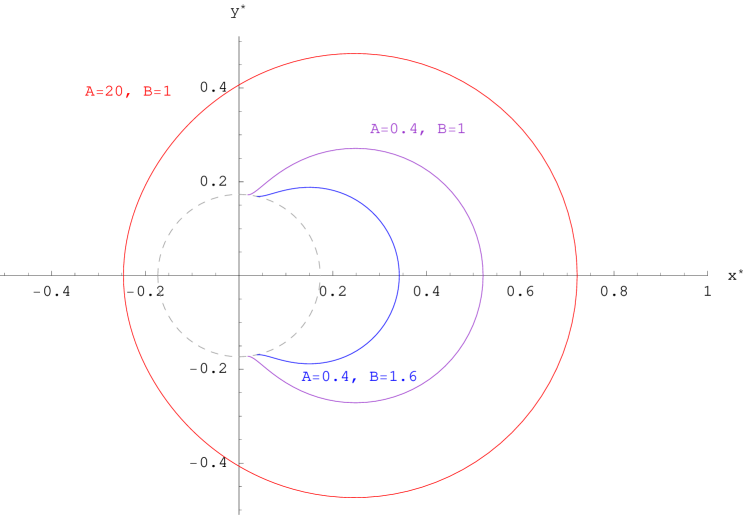
Figure 2: A selection of branes (solid lines) for the case $AB>0$, in a 5-dimensional Schwarzschild bulk of fixed mass parameter $\mu=0.03$. The dashed line denotes the corresponding horizon radius.

$\bullet$ $AB>0$. In this case (52) implies that either the brane completely encloses the event horizon, or it touches (and hence terminates on) the event horizon, depending on the value of $B-A$ compared to the critical value $1/\sqrt{\mu}$. Returning to (47), we see that in the latter case $\cos\chi$ is an increasing function of $r$, and so the brane lies to the right of the points where it touches the event horizon, which are themselves on the right of the $(x^{*},y^{*})$-plane since $B>A$. Figure 2 shows a sample set of brane trajectories in this class. Note that as $\chi^{\prime}<0$ for these trajectories, it is the interior of the bubbles in the bulk that is retained.

For $B>A>0$, it may easily be seen that the energy density (48) remains positive throughout the brane. Turning to (26), we see that this also corresponds to $\rho$ being an increasing function of $r$, hence these branes have an energy surplus at the point located farthest away from the event horizon. The branes terminating on the horizon look like the inside of a bubble, with the event horizon defining its boundary, and its energy density concentrated at its center $\hat{r}=0$. However, the pressure (49) is increasing away from the center of the bubble, eventually acquiring an infinite value at the point where the brane touches the event horizon thus rendering the bubble boundary singular.

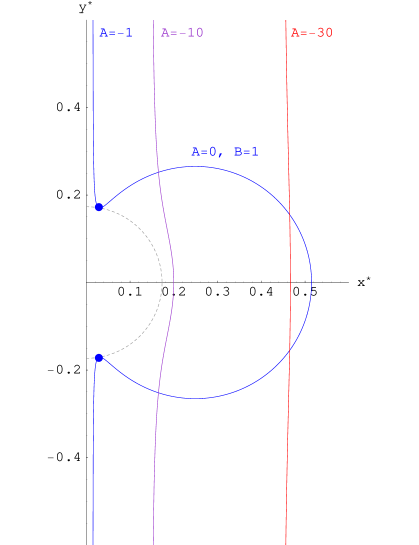
Figure 3: A selection of branes for the case $AB=0$, in a 5-dimensional Schwarzschild bulk of fixed mass parameter $\mu=0.03$. The case $A=0,B=1$ is shown together with a set of branes with $B=0$ and variable $A$. The dashed line denotes again the event horizon.

$\bullet$ $AB=0$. If $A=0$, then (47) will only correspond to a brane exterior to the horizon if $|\cos\chi|=rB\,(1+\sqrt{U})\leq 1$. This leads to the bound $B\leq 1/\sqrt{\mu}$ while positivity of energy demands that $B>0$. Examination of (47) then shows that these trajectories start tangent to the event horizon, curve out into the bulk, then return to the event horizon. The indicative case ($A=0$, $B=1$) is shown in figure 3. The energy density and pressure of these trajectories may be easily shown to be similar to the ones of branes with $AB>0$ terminating on the horizon, and they correspond again to bubbles with a singular pressure boundary.

If $B=0$ on the other hand, the trajectories asymptote $r\cos\chi=-\mu A/2$ at infinity, remaining roughly straight until they near the vicinity of the horizon where they bend away. (Those touching the horizon are the planar solutions of [37].) If $-A<1/\sqrt{\mu}$, then they become tangent to the horizon at the same point as the trajectory, found by swopping $B$ and $-A$. If $-A>1/\sqrt{\mu}$, the trajectories manage to bend sufficiently far that they avoid the event horizon altogether. The borderline case $A=-1/\sqrt{\mu}$ has the brane just skimming the horizon. Figure 3 shows some of these brane trajectories with $B=0$ and variable $A$.

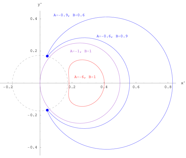
Figure 4: A selection of branes for the case $AB<0$, in a 5-dimensional Schwarzschild bulk of fixed mass parameter $\mu=0.03$. The dashed line denotes again the corresponding horizon radius.

The energy and pressure of these brane trajectories have a particularly simple form :

$$\rho=\frac{-6A}{\kappa_{5}}\left(\sqrt{U}-1\right)^{2}\,,\qquad p=-\frac{\rho}{3}\frac{(\sqrt{U}-1)}{\sqrt{U}}\,.$$ (54)

For $A<0$, these branes have $\rho$ positive and uniformly decreasing as $r$ increases. If $|A|\leq 1/\sqrt{\mu}$, the energy density decreases away from the horizon, however the pressure still diverges there. If $|A|>1/\sqrt{\mu}$, the brane never touches the horizon and the pressure remains everywhere finite. Moreover, the energy density is decreasing away from their centre $\hat{r}=0$, and hence they correspond to asymptotically empty branes with positive mass sources. We will return to these physically interesting cases later.

$\bullet$ $AB<0$. From positivity of energy, we see that here $A$ must be negative, and the brane lies exclusively on the right hand side of the $(x^{*},y^{*})$-plane. The brane can be seen to either be a single arc which touches the horizon, or a closed loop. In fact, by slowly reducing the magnitude of $B-A$, we see that the loop moves closer to the event horizon forming two arcs, each curving away from the horizon, eventually touching it at two points. In this case, the outer half is related to the inner half by exchanging $B\to-A$, and $A\to-B$. A selection of these branes is depicted in figure 4.

For the arc branes with $B-|A|>0$, the energy density increases away from the horizon and reaches its maximum value at the center of the brane $\hat{r}=0$, creating again a bubble with a diverging pressure at its boundary. The same singular behaviour at the event horizon is exhibited by the pressure in the case of arc branes with $B-|A|<0$, although in this case, the energy initially decreases away from the horizon, which corresponds to an energy deficit, and then increases again creating an energy source. In the case of closed loops, that do not touch the horizon, the pressure singularity is again avoided, and the energy density profile resembles one of the two described above depending on the value of $B-|A|$ in that case.

The one exception to the picture described above, where the brane can at most touch the horizon but otherwise it extends outside it, is the special situation alluded to previously, namely the case $A=-B$. The brane equation in this case can be written as

$${y^{*}}^{2}+\left(x^{*}-\frac{1}{4B}\right)^{2}=\frac{1}{16B^{2}}\,.$$ (55)

The above situation is unique in that the brane extends beyond the black hole horizon and even passes through the point mass located at $x^{*}=y^{*}=0$. For this solution the singularity problem associated with crossing the horizon is removed by the choice $A=-B$. The energy density is uniformly increasing with $r$ for $B>0$, and acquires its maximum value at the point located farthest away from the black hole. This type of brane is also shown in figure 4 – the solid purple line indicating the sole trajectory which crosses the horizon.

Having derived these brane trajectories, we would now like to highlight which are likely to be physically useful. First of all, note that the definition of the brane extrinsic curvature means that the normal, defined in (3), is pointing out of the spacetime being kept in this $\mathbb{Z}_{2}$-symmetric identification. This means that, typically, for a trajectory which escapes to infinity, it is the right hand side of the bulk spacetime which is being kept, and for closed branes, it is the interior of the bubble. In other words, for the brane trajectories with $B=0$, the spacetime without the black hole in is the bulk appropriate to the brane trajectory. Similarly, with the small (red) bubble in figure 4, it is the interior of the bubble which is kept, which has no segment of the event horizon in it.

Focussing on the $B=0$ trajectories, as these are asymptotically flat, we now show that these have precisely the energy-momentum one would expect for a TOV star solution. From (54) we see that the energy density is peaked around ${\hat{r}}=r\sin\chi=0$, as is the pressure, the energy falling off as $1/r^{4}$ and the pressure as $1/r^{6}$ (with ${\hat{r}}\propto r$ for large $r$). Plotting the energy and pressure for the brane shows that this does indeed correspond to a localized matter source, with the peak energy density dependent on the minimal distance from the horizon. The central energy and pressure can be readily calculated from this minimal radius, $r_{m}=\mu|A|/2+1/2|A|$:

$$\rho_{c}=\frac{24|A|}{\kappa_{5}(1+\mu A^{2})^{2}}\,,\qquad p_{c}=\frac{16|A|}{\kappa_{5}(\mu A^{2}-1)(1+\mu A^{2})^{2}}\,,$$ (56)

which shows that the central pressure diverges as $\mu A^{2}\to 1$. However, for $|A|=1/\sqrt{\mu}$ the trajectory just touches the event horizon of the black hole, which is the source of this divergent pressure. This is analogous to the divergence of central pressure in the four-dimensional TOV system, which is indicative of the existence of a Chandrasekhar limit for the mass of the star.

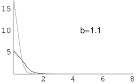
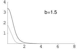
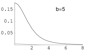
Figure 5: The energy (dark line) and pressure (grey line) of brane stars with a pure Schwarzschild bulk as a function of the brane radial coordinate ${\hat{r}}$. The black hole mass is fixed at $\mu=1$, and the distance of closest approach to the horizon increases across the plots.

Some examples of the solutions to the brane TOV equations are given in figure 5. Notice that as the brane trajectory is moved away from the horizon, the pressure of the matter on the brane decreases; in fact, in the final plot, the pressure can barely be distinguished from the axis. Also note that as $\mu A^{2}$ increases, the spread of the matter on the brane increases. In these spacetimes, there is no actual black hole in the bulk, since it is the bulk to the right of the brane that is retained. Rather, it is the combination of the bulk Weyl curvature and the brane bending which produces the fully coupled gravitational solution.

By working in dimensionless units, $\xi=r/\sqrt{\mu}$ and $b$, we can be more explicit about the dependence of energy on the bulk Weyl mass parameter, $\mu$, and the ‘impact parameter’ $A$ (or $b$). For instance, the energy density on the brane scales as $b/\sqrt{\mu}$, and the spread of the star as $b$. We can also calculate the total mass of the star readily as

$$M_{s}=4\pi\int_{r_{m}}^{\infty}r\rho\,\frac{\sqrt{r^{2}-\alpha^{2}}}{\sqrt{U}}\,dr=\frac{12\pi\mu}{\kappa_{5}}\,F(b)\,,$$ (57)

where $F(b)\to 1$ from above very rapidly. In other words, the total mass of the star is directly proportional to the bulk mass parameter. Referring back to the existence of a central singularity in the pressure, we see that this corresponds to either reducing $b$ to bring the brane to the horizon, or increasing $\mu$, to bring the horizon to the brane (or perhaps a combination of both). In either case, the total mass and the concentration of the matter increases. There is however no overall upper bound on the mass of the star, as we can always have a nonsingular solution for any $\mu$ simply by making $b$ large enough. The limit on mass is therefore not a true Chandrasekhar limit, but more a statement about an upper bound on the concentration of matter. The real reason there is no absolute upper bound is because, unlike the RS system with an adS bulk, gravity on the braneworld is not localized, nor is it four-dimensional. This is also seen in the induced metric on the brane (34), which in the case of a Schwarzschild bulk has no convenient expression in terms of the radial coordinate ${\hat{r}}^{2}=r^{2}-\alpha^{2}$. However, for the one solution which tends to infinity, we see that $\alpha\to\mu|A|/2$, which implies that the asymptotic metric is in fact the projection of the 5-dimensional Schwarzschild metric on the brane.

To sum up: the pure Schwarzschild spacetime has a rich set of brane trajectories, most of which are closed, however, there is a class of asymptotically flat branes which have a localized source satisfying the DEC (mostly) and hence with the interpretation of an isolated gravitating star.

4 Braneworld Stars : A Schwarzschild-adS Bulk

We now turn to the case of a static brane embedded in a 5-dimensional Schwarzschild–anti de Sitter (Sch-adS) spacetime. Since the Randall Sundrum model is a brane in adS spacetime, we expect that any consistent brane trajectories in Sch-adS will potentially correspond to brane stars or black holes. It is worth stressing that these solutions will not just be brane solutions, but full brane and bulk solutions, since the full Israel equations for the brane have been solved in a known bulk background.

Note that in the Randall-Sundrum scenario, our empty brane solution does not have zero energy-momentum, but a background constant energy and tension: $T_{\mu\nu}=\rho h_{\mu\nu}$, where $\rho=\rho_{RS}$ for the critical RS brane, and $\rho<\rho_{RS}$ for the subcritical Karch-Randall brane. Therefore, when we compute $p$ and $\rho$ for a spherically symmetric brane, this background brane energy momentum will be included. According to [21], the brane gravitational field couples to the differential energy momentum

$${\cal T}_{\mu\nu}=T_{\mu\nu}-\frac{\rho_{b}}{\kappa_{5}}h_{\mu\nu}$$ (58)

where $\rho_{b}$ is the background brane tension, as well as a possible brane cosmological constant term corresponding to the difference between $\rho_{b}$ and the critical RS brane tension. For the critical brane, ${\cal T}_{\mu\nu}$ will give the extra matter on the brane which is sourcing the spherically symmetric gravitational field, however, sub- and super-critical branes will also have an additional gravitational effect from the cosmological constant term. For the sake of simplicity, as well as correspondence with the zero bulk black hole mass limit, we will identify the background brane tension as

$$\rho_{b}=\frac{6k(a-b)}{\kappa_{5}\sqrt{1-4ab}}$$ (59)

The metric function $U(r)$ is now given by

$$U(r)=1+k^{2}r^{2}-\frac{\mu}{r^{2}}\,,$$ (60)

and is not covered by the general metric ansatz studied in the previous section. The function $\tilde{r}$ actually has an exact analytic expression

$${\tilde{r}}(r)=\frac{1}{kr_{+}}\,{\rm Elliptic\,F}\left[{\rm Arcsin}\left(\frac{r}{r_{-}}\right),\frac{r_{-}^{2}}{r_{+}^{2}}\right]\,.$$ (61)

In the above, $r_{+}$ (the black hole horizon) and $r_{-}$ are defined by the expressions

$$r_{+}^{2}=\frac{-1+\sqrt{1+4k^{2}\mu}}{2k^{2}}\,,\qquad r_{-}^{2}=\frac{-1-\sqrt{1+4k^{2}\mu}}{2k^{2}}\,.$$ (62)

Although an exact solution, the expression (61) is of limited use because of the imaginary value of $r_{-}$, and the presence of the Elliptic function. It can be used of course to give numerical solutions for the brane, as we will do presently, however we will first deduce some general properties of trajectories based in part on what we have learned from the effects of the black hole mass, and negative cosmological constant separately.

First of all, note that for large enough $r$, the geometry will be dominated by the cosmological constant, therefore we expect that our pure adS solutions will be good approximations to any trajectories for large $r$. Next, if $\mu k^{2}\ll 1$, i.e. if the black hole is much smaller than the adS scale, we expect that in the vicinity of the horizon the Schwarzschild solutions will be good approximations for the brane, therefore for small mass black holes, we might expect brane trajectories to be well approximated by some combination of Schwarzschild and adS branes. We would like to note here that, for convenience and easy comparison with the pure adS limit, we zero the $\tilde{r}$-coordinate at infinity. Then, the range of $\tilde{r}$ in Sch-adS turns out to be finite, and to decrease sharply with increasing $\mu$ (for example, if $\mu=0.01$, $r_{+}\simeq 0.1$ and ${\tilde{r}}_{+}\simeq-3.7$, whereas if $\mu=10^{5}$, $r_{+}\simeq 10$ and ${\tilde{r}}_{+}\simeq-0.13$). This suggests that trajectories in large mass Sch-adS black hole spacetimes are more finely tuned, and possibly more restricted than in small mass black hole spacetimes.

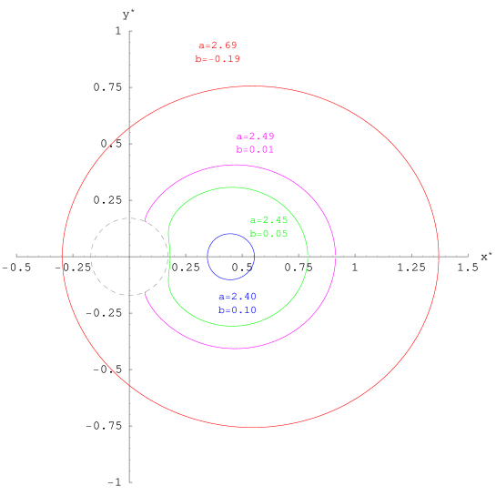
Figure 6: A sample of supercritical brane trajectories with $a+b>1$ in a 5-dimensional Schwarzschild–anti de Sitter background of fixed parameters $k=1$ and $\mu=0.03$. The dashed line denotes again the horizon.

We are clearly interested in branes which have matter that can be interpreted as a gravitating source, i.e. we would like to have a energy excess at the center of the brane. We can see therefore that, unless we have a closed bubble, this will in general correspond to $\rho$ being an increasing function of $r$. From (26), we see that in Sch-adS

$$\rho^{\prime}=\frac{2\mu\rho_{0}}{r^{3}}\,(\cos\chi)^{\prime}\,,$$ (63)

hence $\rho$ will be a decreasing function of $r$ if $\cos\chi$ is. However, from (32), $\rho$ is asymptotically dominated by $\rho_{0}\sqrt{U}(ae^{\tilde{r}}-be^{-{\tilde{r}}})/r\propto(\cos\chi)^{\prime}$, hence any positive energy brane trajectory will have $(\cos\chi)^{\prime}>0$ near infinity, and hence $\rho$ will be increasing near infinity (albeit at a very slow rate), corresponding to an energy deficit at large $r$. However, this underdensity will prove to be extremely marginal, and many trajectories have, as their main feature, energies significantly in excess of their background value in the interior.

Like adS spacetime, the Sch-adS trajectories can be classified according to whether they asymptote the adS boundary at nonzero $\chi$, at $\chi=0$, or do not reach the boundary at all, i.e. are closed bubbles. These correspond to subcritical, critical, or supercritical branes ($a+b>1$, $a+b=1$, and $a+b<1$) respectively.

4.1 Supercritical branes

We will now show that all closed trajectories are supercritical. Clearly if a trajectory is not closed, it is not supercritical, since if a brane asymptotes the adS boundary, then in that asymptotic regime it must have $|\cos\chi|\simeq|a+b|\leq 1$ from the pure adS results. Now suppose that the brane has a finite extent. In that case, the brane must satisfy $\cos\chi=1$ at some value ${\tilde{r}}_{1}<0$. If the brane is closed, it should also satisfy $\cos\chi=\cos\chi_{0}$ at some other value ${\tilde{r}}_{0}<\tilde{r}_{1}$, where $\chi_{0}=0$ if the bubble lies entirely on the RHS of the black hole, and $\chi_{0}=\pi$ if the bubble encloses the black hole. The only other possibility for a finite brane is to terminate on the horizon and, in that case, ${\tilde{r}}_{0}={\tilde{r}}_{h}$ if $\chi_{0}\in(0,\pi)$. Using this information, we find that

$$a=\frac{e^{{\tilde{r}}_{1}}-e^{{\tilde{r}}_{0}}\cos\chi_{0}}{e^{2{\tilde{r}}_{1}}-e^{2{\tilde{r}}_{0}}}\,,\qquad b=e^{{\tilde{r}}_{1}+{\tilde{r}}_{0}}\frac{(e^{{\tilde{r}}_{1}}\cos\chi_{0}-e^{{\tilde{r}}_{0}})}{e^{2{\tilde{r}}_{1}}-e^{2{\tilde{r}}_{0}}}\,.$$ (64)

From the above we may see that, since ${\tilde{r}}_{0}<{\tilde{r}}_{1}<0$, $a+b$ is a decreasing function of ${\tilde{r}}_{1}$; therefore, since $a+b=1$ for ${\tilde{r}}_{1}=0$, $a+b>1$ for a closed bubble with $\tilde{r}_{1}<0$.

In figure 6, we depict a sample of supercritical branes for fixed background parameters $k=1$ and $\mu=0.03$, and various values of the parameters $a$ and $b$ of the general solution (30). The branes exhibit the features discussed above and form either closed loops or arcs terminating on the horizon. The latter characteristic is determined by whether $a$ and $b$ satisfy the constraint $|\cos\chi|\simeq|ae^{\tilde{r}_{+}}+be^{-\tilde{r}_{+}}|\leq 1$ near the horizon. For the arcs terminating on the horizon, it may be easily seen that the energy density remains positive and increases towards the center of the brane. As in the Schwarzschild case, however, the pressure becomes singular at the horizon. For branes forming a closed loop on the RHS of the horizon, a similar behaviour is found to the one encountered in the Schwarzschild background: the energy density decreases near the vicinity of the horizon but increases towards the most distant point of the brane. A uniformly increasing behaviour for the energy density is found also in the case of brane trajectories that enclose the black hole horizon: $\rho$ reaches its maximum positive value at the point of the brane located farthest away from the black hole, although care must be taken over the choice of $a$ and $b$ to ensure that $\rho$ remains positive throughout the trajectory.

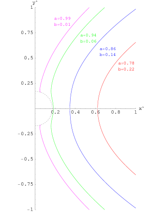
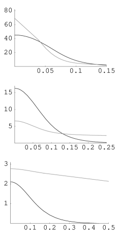
Figure 7: (a) A sample of critical brane trajectories with $a+b=1$ in a 5-dimensional Schwarzschild–anti de Sitter background of fixed parameters $k=1$ and $\mu=0.03$. The dashed line denotes again the horizon. (b) A set of plots of the brane energy (black line) and pressure (grey line) for a sequence of critical branes moving away from the horizon.

4.2 Critical branes

In this case we have $a+b=1$, which means that the brane trajectories asymptote the adS boundary at exactly $\chi=0$. The branes are thus open, and may or may not touch the black hole horizon depending on the exact values of the parameters $a$ and $b$. In order to demonstrate when this happens, we describe our trajectories in terms of a sole parameter by writing $a=(1+c)/2$ and $b=(1-c)/2$. Then, if

$$c<|\tanh{\tilde{r}}_{+}/2|\,,$$ (65)

the trajectory will remain on the RHS of the horizon: after reaching a point of closest proximity, the brane will bend to avoid the horizon and eventually escape to infinity. If $c$ saturates or exceeds the above bound, the brane will terminate on the horizon. A sample of critical trajectories in a Sch-adS background is shown in figure 7(a).

The behaviour of the energy density and pressure in this case is strongly dependent on the location of the brane compared to the black hole. Branes that originate from the horizon and extend to infinity have their energy density positive, provided they intersect the horizon at $\chi_{0}<\pi/2$, i.e. $c<|\coth{\tilde{r}}_{+}|$. The horizon is then a local energy maximum if $c<|\tanh{\tilde{r}}_{+}|$, with the energy decreasing away from the horizon, undershooting the asymptotic value before increasing again towards the asymptotic critical value. If $c>|\tanh{\tilde{r}}_{+}|$, then the energy monotonically increases out to infinity. In addition, the pressure, as expected, diverges at the black hole boundary.

According to figure 7(a), as the value of the $c$ parameter decreases, the brane shifts towards the right. For branes that avoid the horizon the energy density is again positive, peaking at the center, and dropping rapidly to the background value, undershooting it slightly to form the underdense region already discussed. The pressure also reaches its maximum value at the center, but is uniformly decreasing with $r$, at a much slower rate, consistent with the pressure excess observed for the pure adS branes. Apart from this pressure excess, the other main difference with pure Schwarzschild trajectories, is whether branes satisfy the differential DEC at their center depends crucially on the choice of $c$. By differential DEC, we mean the DEC for the differential energy momentum ${\cal T}_{\mu\nu}$, and thus the energy momentum tensor for an observer on the brane. In pure Schwarzschild, the DEC is satisfied except for branes which skirt extremely close to the horizon, where the local Weyl curvature causes the pressure to diverge. This phenomenon is also observed for the Sch-adS branes skimming close to the horizon, however, as we decrease $c$ (or increase $b$) the central energy dominates the pressure for only a finite range of $b$ before once again dropping below the pressure. This is because the further we move away from the horizon the adS curvature becomes more important, and for pure adS branes, the effect of the adS curvature is to induce a pressure excess. In figure 7(b), we present the (differential) energy density and pressure for a sequence of critical branes in a Sch-adS background displaced an increasing distance from the horizon. One may easily observe the localization of both the energy density and pressure at the center of the brane, corresponding to a distribution of a positive mass source, as well as the fact that the DEC can be satisfied at the centre of the distribution.

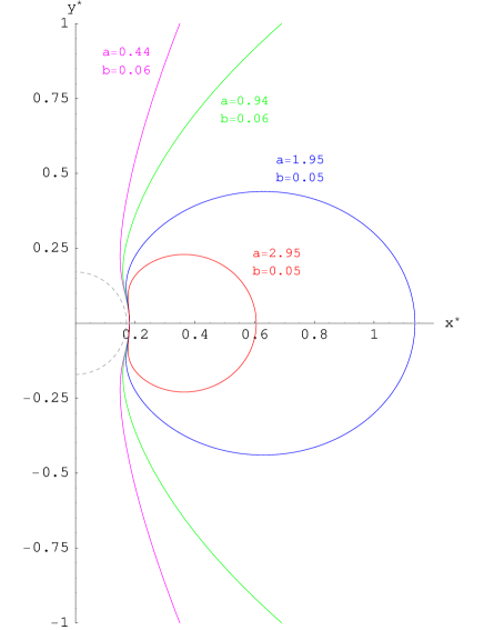
Figure 8: A mixture of brane trajectories in a 5-dimensional Schwarzschild–anti de Sitter background of fixed parameters $k=1$ and $\mu=0.03$.

4.3 Subcritical branes

This family of branes with $a+b<1$ are largely similar to critical branes. They correspond to open trajectories that asymptote the adS boundary, although at nonzero $\chi$ in this case. The same bound as before, i.e. whether $|\cos\chi|\simeq|ae^{\tilde{r}_{+}}+be^{-\tilde{r}_{+}}|\leq 1$, will determine whether the brane terminates on the event horizon or remain on the RHS of it. As the brane trajectories in this case look similar, apart from the angle of approach from the adS boundary, to the ones presented in figure 7(a) for critical branes, we refrain from presenting another graph here. The energy density and pressure profile in this case is again similar to the one found for critical branes. Once again, for a large family of parameters $a$ and $b$, solutions with a positive energy excess at the center of the brane may be easily found.

One special subcritical trajectory found in the pure adS case was the Karch Randall trajectory, $a+b=0$. We can extend this to Sch-adS obtaining

$$\cos\chi=2a\sinh{\tilde{r}}$$ (66)

however, since $a>0$ for a positive energy trajectory, this has $(\cos\chi)^{\prime}>0$, and hence the energy density is always increasing with $r$. Thus, whether or not these trajectories terminate on the horizon, they always correspond to energy deficits on the brane, and hence negative mass sources from the point of view of a brane observer.

Finally, one other special trajectory that emerged from the previous section was the Schwarzschild trajectory which was nonsingular on the horizon, intersecting it perpendicularly and extending to the origin. This corresponds to $ae^{{\tilde{r}}_{+}}=be^{-{\tilde{r}}_{+}}$ (note that the condition $A=B$ for Schwarzschild was for an ${\tilde{r}}$ coordinate zeroed at the horizon). Extending this concept to Sch-adS gives

$$\cos\chi=2ae^{{\tilde{r}}_{+}}\cosh({\tilde{r}}-{\tilde{r}}_{+})$$ (67)

These trajectories can be super- sub- or precisely critical, depending on the magnitude of $a$, however, for all of these trajectories $(\cos\chi)^{\prime}>0$, hence they correspond to energy deficits on the brane.

The brane trajectories found in this section and depicted in figures 6 and 7 have obvious similarities with the ones presented in the previous section. As expected, the brane trajectories in a bulk containing both a mass and a negative cosmological constant are hybrid constructions, and exhibit features and characteristics that appeared either in the case of an adS or a Schwarzschild background. As an example, in figure 8, we present a mixture of supercritical, critical and subcritical branes embedded in a Sch-adS bulk, that clearly resembles the one presented in figure 1. The parameters $a$ and $b$ in this particular case have been chosen so that the branes remain on the RHS of the horizon, and apart from the brane bending to avoid the horizon, these trajectories have otherwise similar characteristics with the ones in figure 1. Finally, we would like to note here that the study of Sch-adS backgrounds with larger mass parameter $\mu$ has led to similar families of trajectories. As mentioned earlier, as the value of $\mu$ gets bigger, the range of the $\tilde{r}$-coordinate becomes shorter, and an increased accuracy is necessary in our numerical analysis in order to produce the corresponding trajectories. Apart from being numerically more sensitive, the study of large mass Sch-adS backgrounds yields the same characteristics for the allowed brane trajectories.

5 The Time-Dependent Brane

Having analysed the static brane trajectories in a spherically symmetric background, finding brane black hole and stellar solutions, we now comment on the time dependent case. The full problem is beyond the scope of this paper, however, we will make some remarks here, and explore the various issues involved in finding a time-dependent brane black hole trajectory, such as might be appropriate to black hole evaporation or recoil.

5.1 Exact branes

We start by reviewing the argument that there is no time-dependent trajectory which corresponds to a pure vacuum brane embedded in a black-hole bulk background. Setting $v=-1$ in the brane equations (2)-(22) results in considerable simplifications. Once again, the energy density

$$\rho=\frac{\rho_{0}}{r^{2}}\,\left[U(\alpha^{\prime}r-\alpha)+\alpha\right]\,,$$ (68)

(which in principle can be a $(\tau,r)$-dependent quantity) solves (21) and (22). In addition, (19) is immediately integrable yielding

$$\alpha(\tau,r)=f(\tau)\,\sqrt{U(r)}+g(r)\,,$$ (69)

where $f(\tau)$ and $g(r)$ are, at the moment, arbitrary functions. If we substitute the above form of $\alpha(\tau,r)$ into (18), we then find

$$\sqrt{U}\left(\frac{1}{2}\,U^{\prime\prime}r^{2}-U^{\prime}r+U-1\right)f(\tau)+Ur^{2}g^{\prime\prime}+(g^{\prime}r-g)\left(\frac{U^{\prime}r}{2}-U\right)-g=0.\,$$ (70)

The only way for this equation to be satisfied, for all $\tau$, with $f(\tau)\neq 0$, is for the factor preceding $f(\tau)$ to be equal to zero:

$$\frac{1}{2}\,U^{\prime\prime}r^{2}-U^{\prime}r+U-1=0\,,$$ (71)

which has as a solution

$$U(r)=1+Cr+Dr^{2}\,,$$ (72)

for constants $C$ and $D$. Thus a brane with equation of state $w=-1$ can only be embedded in a bulk with the above solution for the metric function. However, computing the energy momentum tensor of the bulk spacetime, and demanding that it be isotropic leads to $C=0$, and hence a constant curvature spacetime with $D=-\Lambda/6$. Clearly adS spacetime satisfies this, with $D=k^{2}$. Here the pure tension brane trajectory takes the form

$$\alpha(\tau,r)=\frac{1}{k}\,\sqrt{1+k^{2}r^{2}}\,\cos(k\tau)-\frac{1}{k}\,,$$ (73)

with energy, as expected,

$$\rho=\rho_{RS}=\frac{6k}{\kappa_{5}}\,.$$ (74)

This is the Randall-Sundrum brane in global coordinates. To see this, use the transformation between global adS and RS coordinates:

$$ku = \left[\sqrt{1+k^{2}r^{2}}\cos k\tau-kr\cos\chi\right]^{-1}$$ (75)

$$kt = \left(ku\right)\sqrt{1+k^{2}r^{2}}\ \sin k\tau$$ (76)

$$k|{\bf x}| = \left(ku\right)kr\sin\chi\,,$$ (77)

in which the RS metric is:

$$ds^{2}=\frac{1}{k^{2}u^{2}}\left[-dt^{2}+du^{2}+d{\bf x}^{2}\right]\,.$$ (78)

The wall trajectory in global coordinates is in fact oscillatory, starting off at the adS boundary, moving in to the origin when it closes off the whole adS boundary, then moving back again. The RS wall is oscillatory because the spherical coordinates are the universal covering space of adS, and so the ‘wall’ is actually an infinite family of walls, each in the local patch covered by the horospherical coordinates.

The key feature of this wall trajectory is that it satisfies the Israel junction conditions [39] for a ‘brane’ energy-momentum tensor which is proportional to the induced metric on the brane. A natural generalization of this situation would be the consistent embedding of a brane, with a general energy-momentum tensor, in a bulk background that describes a regular black hole in either flat or curved spacetime.

5.2 Branes with matter

Let us now explore simplistically what happens if we modify the global adS metric to Sch-adS. Since $r=0$ is a geodesic of the spherical adS spacetime, the image of $r=0$ in the Randall-Sundrum spacetime, which is a hyperbola, will be a geodesic in the RS spacetime. Therefore, if we put a black hole at $r=0$, it should look like a particle in the RS spacetime, at least to a first approximation. We should note here that this philosophy is similar to that of [38], who considered slices of Sch-adS which would satisfy the DEC. However, note that those slices were static (and asymptotically adS), crucially here we are allowing time dependence in order to get an asymptotically flat brane, as well as the interpretation of black hole evaporation or recoil

As we have just shown, it is not possible to have a vacuum brane embedded in anything other than pure adS spacetime, therefore finding a full solution to a time-dependent braneworld black hole would require embedding a time-dependent axisymmetric brane at the very least in an axisymmetric bulk, since it was proven in [11] that a bulk with SO(4) symmetry must necessarily be Sch-adS. Thus, the exact solution for the vacuum brane is an extremely involved problem which is probably only tractable numerically. What we will now do is to relax the assumption that $T_{\mu\nu}\propto h_{\mu\nu}$ for the brane, and explore the effect of the bulk black hole on the time-dependent brane, determining the effect of brane bending and varying the brane position and black hole mass on the brane energy-momentum.

From (75), we see that a flat brane sitting at $ku=\epsilon$ in the RS picture satisfies

$$\sqrt{1+k^{2}r^{2}}\cos k\tau-kr\cos\chi=(ku)^{-1}=\frac{1}{\epsilon}\,.$$ (79)

Therefore as a starting point, we keep this same trajectory and calculate the energy-momentum. As we have already discussed, there is no trajectory that will have a pure brane energy momentum, $T_{\mu\nu}=-(6k/\kappa_{5})\,h_{\mu\nu}$, however, as a black hole formed on the brane must be produced by the collapse of matter, it is not clear whether we should expect a pure brane energy momentum solution; rather, a solution corresponding to the collapse of matter on the brane is perhaps more physically realistic.

The aim of this subsection is to understand how the bulk black hole acts on the brane energy momentum, producing a spherically symmetric brane matter source. By varying the black hole mass, the distance of closest approach of the black hole to the brane, and modifying the brane trajectory, we can study the effect of these various factors on the brane energy momentum. Since we expect the full picture to involve all three of these effects in some combination, this process of isolating the effect of each will allow us to gain insight into the nature of the brane black hole. Unlike the previous sections however, here we are not imposing a particular type of matter, such as an isotropic fluid, but determining whether time-dependent brane trajectories exist which have sensible matter on the brane. In particular, we will be looking for matter which obeys the weak energy condition (WEC), namely that the energy density increases at the center of collapse.

Recall that the energy momentum of a surface slicing the Sch-adS spacetime is given by the Israel junction conditions as:

$$T_{\mu\nu}=\frac{2}{\kappa_{5}}\left(K_{\mu\nu}-Kh_{\mu\nu}\right)=-\frac{6k}{\kappa_{5}}\,h_{\mu\nu}+t_{\mu\nu}\,,$$ (80)

where we have taken the critical RS brane tension $6k/\kappa_{5}$, and $t_{\mu\nu}$ is (hopefully) a small perturbation in the energy-momentum. We can compute this geometric energy momentum from (11-14), and since we want to compare this to a pure critical RS brane $T_{\mu\nu}=-(6k/\kappa_{5})\,h_{\mu\nu}$ we will plot the ratio (in an obvious abuse of notation):

$$e_{\mu\nu}=\frac{(K_{\mu\nu}-Kh_{\mu\nu})}{(-h_{\mu\nu})}=\frac{T_{\mu\nu}}{(-2h_{\mu\nu})}=3+\frac{t_{\mu\nu}}{(-2h_{\mu\nu})}\,.$$ (81)

In the above, we have set for simplicity $\kappa_{5}=1$. Clearly, since the trajectory is time dependent, this ratio will also be time dependent, however, we expect that the largest effect of the bulk black hole will be represented by the $t=0$ slice of the braneworld – the point of closest proximity – we therefore plot the energy momentum at $t=0$. This has the simplifying effect of making ${\dot{\chi}}=0$ in the expressions for the extrinsic curvature, and gives a local static frame for the energy momentum tensor.

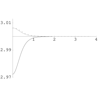
Figure 9: The energy-momentum of an RS brane with a black hole in the bulk as a function of the brane radial coordinate $r\sin\chi$. The energy is given by the black line, the radial pressure by the grey line and the azimuthal pressure by the dotted line.

Figure 9 shows the effect of the bulk black hole on the energy momentum tensor of the brane. We have picked a small bulk black hole ($\mu=0.1$), and the RS brane sits at $ku=0.3$. The energy is the solid black line, the radial tension the grey line, and the angular tension the dotted line. The black hole causes the energy of the brane to decrease from its critical value, whereas both the radial and azimuthal tension increase. Clearly, therefore, from the point of view of differential energy-momentum, this brane does not satisfy the WEC, although the overall energy momentum does satisfy the WEC. The brane however fails to satisfy the dominant energy condition (DEC). Unsurprisingly, moving the RS brane towards the black hole increases the overall effect on the energy and tension. Increasing the mass of the black hole in the interior changes this picture surprisingly little, provided we simultaneously move the RS brane towards the boundary.

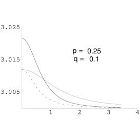
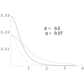
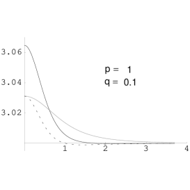
Figure 10: A selection of plots of brane energy-momentum with brane bending included for a range of amplitudes and powers of $r$.

Clearly therefore, maintaining the RS slicing of the global spacetime in the presence of a black hole results in brane energy momenta which are not physically sensible, they satisfy neither brane WEC nor DEC. However, this was not unexpected, as we have not modified the RS trajectory, and the main feature of our static brane solutions was that they responded to the bulk black hole by bending. Indeed, in a definitive brane gravity paper, [9], Garriga and Tanaka showed that a crucial part of obtaining four dimensional Einstein gravity (i.e. with the correct tensor structure) was what could be interpreted as a brane bending term. Essentially, the effect of matter on the brane was to “shift” the brane with respect to the acceleration horizon in the bulk. Clearly then, if a black hole forms on the brane, we would expect the brane to respond to this matter by bending. The $1/r$ brane bending term derived in [9] was of course in the static limit, therefore we cannot simply read off what the non-static term should be, therefore we try a variety of modifications to the position of the brane to explore their effect.

A shift in the position of the brane corresponds to $ku\to 1+k\delta u$, and we will make the simplifying assumption that $k\delta u=-\delta(r)$, trying out a range of functions $\delta$:

$$\delta(r)=\frac{q}{r^{p}}\,.$$ (82)

What this does is to change the function $\chi$:

$$\cos\chi(\tau,r)=\frac{1}{r}\left(\sqrt{1+r^{2}}\ \cos\tau-\frac{1}{u}\right)\simeq\frac{1}{r}\left(\sqrt{1+r^{2}}\ \cos\tau-\frac{1}{1+\delta(r)}\right)\,,$$ (83)

where we can use the transformation between RS and global coordinates to try out a range of power laws in $\delta(r)$ which reduce to sensible brane bendings in the RS picture.

We have looked at the effect of bending the brane both towards and away from the black hole for a variety of $\delta(r)$. In all cases, bending the brane towards the black hole worsens the energy deficit on the brane, and does not help with the DEC. However, bending the brane away from the black hole, as occurs in the static brane trajectories, can remove the energy deficit, and indeed restore the DEC near the centre of the brane. This indicates that a true brane trajectory will try to avoid the black hole by bending away from it.

Figure 10 shows the effect of the brane bending on the energy-momentum. Bending the brane by a power $p>1$ introduces an energy deficit at some radius, therefore we only show those functions which maintain the differential brane WEC. The GT brane bending of $1/x$ corresponds approximately to $p=1/2$.

Finally, we point out that unlike the static trajectories, in these time dependent cases the black hole is in the bulk spacetime, hence these are candidate branes for a black hole having recoiled into the bulk.

5.3 The interaction of black holes and branes

The main motivating factors for obtaining a time-dependent braneworld black hole are to gain insight into the back-reaction of Hawking radiation on a quantum corrected four-dimensional black hole, and to understand the process of black hole recoil from a braneworld. In the former case we would want a $\mathbb{Z}_{2}$-symmetric solution, while the latter case does not necessarily require this. Since we have been working within the $\mathbb{Z}_{2}$-symmetric setup, we will only consider this here.

The idea is that the time-dependent process will be some perturbed version of a time-dependent brane trajectory in five-dimensional Sch-adS spacetime. By allowing the brane to intersect the bulk black hole horizon, this would appear to describe black hole formation and evaporation via transport of a bulk black hole to the brane, and subsequent departure back into the bulk. When the brane hits the black hole, we might expect some part of it will be captured by the black hole, and will therefore remain behind the event horizon even when the black hole has left the brane, effectively having been chopped off from the rest of the brane. This feature is seen in the probe brane calculations of [41], and we expect this to hold in the case of a fully gravitating brane. In support of this, we can appeal to the case of a cosmic string interacting with a black hole, where early work indicated that strings would be captured, and via self-intersection would leave some part behind in the black hole [42], and idealized gravitational calculations show explicitly how this ties in with the thermodynamic process of string capture and black hole entropy [43]. Just as in the cosmic string case, this capture of the brane by the black hole will turn out to be important in establishing the thermodynamic viability of the black hole recoil process.

The recoil of the black hole from the brane is an important indicator of the possible evaporation process. Since the energy-momentum on the brane violates the DEC, it might be thought that this is an indicator that the black hole cannot leave the brane, and indeed a naive entropy argument supports this view. The argument runs as follows: A black hole of mass $M$ on the brane has entropy $\sim M^{3/2}$, however, if it recoils into the bulk, it must recoil as two black holes of mass $M/2$, hence total entropy $2(M/2)^{3/2}=M^{3/2}/\sqrt{2}$. Thus black hole recoil is entropically forbidden. However, there are some interesting possible corrections to this simple argument, that can change this equation rather substantially. First, at the calculational level, the fact that entropy is proportional to horizon area/volume, which for Sch-adS is not simply related to the mass. Next, it does not take into account the effect of the brane bending. Since the brane is bent, if it does intersect the black hole horizon, it will not do so at the equator, but somewhat “south”, i.e. for $\chi_{0}>\pi/2$. For the black hole intersecting the horizon at $\chi_{0}$, the actual area contributing to the entropy of the intermediate state is

$${\cal A}_{int}=4\pi f(\chi_{0})\left[\frac{\sqrt{1+2\pi k^{2}\mu/f(\chi_{0})}-1}{2k^{2}}\right]^{3/2}\,,$$ (84)

where $f(\chi)=\chi/2-(\sin 2\chi)/4$.

Finally, in the process of the black hole intersecting the brane, we would expect some part of the brane to be excised and captured by the black hole, thus increasing its mass. Estimating this as

$$\delta M=\frac{6k}{\kappa_{5}}\frac{4\pi}{3}(r_{+}\sin\chi_{0})^{3}\,,$$ (85)

we see that the area of the final state is in fact

$${\cal A}_{f}\simeq{2\pi^{2}}\left[\frac{\sqrt{1+4k^{2}\mu+32k^{3}(r_{+}\sin\chi_{0})^{3}/3\pi}-1}{2k^{2}}\right]^{3/2}\,.$$ (86)

The above becomes larger than the intermediate area at $k^{2}\mu\simeq 0.01$ for $\chi_{0}\leq\pi/4$, and even ignoring the brane bending effect by setting $\chi_{0}=\pi/2$, we still find that black hole recoil is preferred at $k^{2}\mu\geq 0.07$, or at a (four-dimensional) Schwarzschild radius

$$2G_{N}m\simeq l_{\,adS}/10$$ (87)

where $l_{\,adS}$ is the adS length scale.

It is important to note that these arguments use the standard entropy of the isolated Sch-adS black hole. In other words, they assume a static solution with an event horizon at $r_{+}$. Clearly in the time-dependent spacetime there is some question about whether this approximation is valid, indeed, even ignoring branes, we see that a black hole with mass greater than about $3$ (in adS units) has lower entropy than two black holes of mass $3/2$. Clearly therefore, entropy arguments should be used with caution, nonetheless, for small black holes, where we might expect them to be more reliable, taking into account brane bending and fragmentation shows that it is by no means entropically preferred for a black hole to stick to the brane.

To sum up: taking time dependent brane trajectories in a Sch-adS background give brane trajectories with additional matter on the brane. The brane prefers to bend away from the black hole, and in such a case the matter satisfies the DEC near the core of collapse, and the WEC at all times. For very small black holes ($\mu k^{2}\leq 0.01$) our results suggest that the bending of the brane may cause it to avoid the black hole altogether. We cannot use our approximation to draw conclusions for large black holes, as it presupposed the black hole was a small perturbation to the RS spacetime. The entropy argument for black hole recoil supports the notion that part of the brane will be captured by the black hole, however, we have not attempted to model this gravitationally with time dependent closed branes at this point. Clearly any more detailed calculation would require modification of the bulk solution.

6 Conclusions

In this work, we have analyzed spherically symmetric brane solutions in a known bulk spacetime with the aim of finding a consistent black hole solution for the brane. We found that the problem of a static braneworld slicing a known spherically symmetric bulk was completely integrable, with the solution being given in terms of an implicit function of the bulk radial variable. Thus, we have found all possible complete brane and bulk solutions for a brane with a perfect fluid matter source living on it – in other words complete brane TOV solutions. These solutions have the interpretation of braneworld stars, and correspond to static slicings of a Sch-adS bulk spacetime, with the bulk solution corresponding to the part of the Sch-adS spacetime not containing the event horizon of the black hole. Thus our solutions are completely nonsingular. We have also found solutions in which the event horizon of a bulk black hole impinges upon the brane, but these typically have divergent pressure on the brane, reminiscent of the singularity in the TOV system when we try to solve for too big or compact a star.

All of our solutions contain excess pressure at large radii, this seems to be a feature of the slicing of the pure adS bulk, and it is related to the fact that the Randall-Sundrum solution, a pure Minkowski brane, is in fact not a static slicing of adS in global coordinates. The only possibility for having a well-behaved asymptopia is to have a subcritical Karch-Randall brane. These however, cannot be extended into positive mass sources. We have therefore been unable to find a solution which has all the features we would desire in a braneworld star, however, we have made crucial progress by first demonstrating how to find exact and complete solutions to the brane TOV problem, as well as classifying these according to their energy-momentum.

Probe brane calculations of the interaction of a wall with a black hole indicate the possibility of brane excision, that is, that as the black hole leaves the brane, the brane is distorted so much that it self-intersects and part of the brane is excised, falling into the black hole, with the remainder moving away towards infinity. Among our various solutions are closed bubbles as well as open branes, and it is tempting to try to model this process using a quasi-static approach – taking a sequence of the static solutions we have found as approximate solutions (such as in [44]). Unfortunately however, positivity of energy requires that the interior of the bubbles be kept, and for the branes extending to infinity, the bulk does not contain a black hole, therefore these solutions are not suitable for such an approximation. If we wished to keep the exterior of the bubble and the black hole inside the bulk spacetime, we would need negative energy branes. It would appear that time-dependence is key to finding consistent solutions, as in those cases, the black hole is actually retained in the bulk.

We have also explored the time dependent brane trajectories, using the RS brane as a starting point, to try to model the process of gravitational collapse, and to explore the issues involved in black hole evaporation. We found that the effect of a bulk black hole on the RS brane was to induce a negative energy source, however, by bending the RS brane by a small amount, we could restore the brane-DEC, although these solutions had anisotropic pressure. Provided we allow matter on the brane, we can form trajectories which now have black holes in the bulk, and which can intersect with the brane, although in this case the DEC is violated.

Finally, an important point to note is that in all our results, we have made the simplifying assumption of $\mathbb{Z}_{2}$-symmetry around the brane. The RS model is $\mathbb{Z}_{2}$-symmetric, and many of the investigations into gravitational braneworld solutions are also $\mathbb{Z}_{2}$-symmetric. However, it is obviously important to check and explore if any of our conclusions change significantly if we drop this restriction. In particular, for black hole recoil off the brane, we would expect the black hole to recoil on one side only of the brane, and hence for $\mathbb{Z}_{2}$-symmetry to be broken. It may be that many of the restrictions we have found with our solutions can be evaded if we remove $\mathbb{Z}_{2}$-symmetry. This is currently under investigation.