Symmetry Aspects in Nonrelativistic Multi-Scalar Field Models and Application to a Coupled Two-Species Dilute Bose Gas

Abstract

We discuss unusual aspects of symmetry that can happen due to entropic effects in the context of multi-scalar field theories at finite temperature. We present their consequences, in special, for the case of nonrelativistic models of hard core spheres. We show that for nonrelativistic models phenomena like inverse symmetry breaking and symmetry non-restoration cannot take place, but a reentrant phase at high temperatures is shown to be possible for some region of parameters. We then develop a model of interest in studies of Bose-Einstein condensation in dilute atomic gases and discuss about its phase transition patterns. In this application to a Bose-Einstein condensation model, however, no reentrant phases are found.

,

Published: J. Phys. A: Math. Gen. 39, 6687 (2006)

1 Introduction

One of the most interesting aspects concerning the studies of multi-field models at finite temperature is the possibility of emergence of a much richer phase diagram than one would usually find in one field type of models. The possibility that unusual symmetry patterns could emerge in those models, for some specific region of parameters, has attracted considerable attention in the literature (see, for instance, [1, 2] and references therein and [3] for a short review).

For most of the standard physical systems we know in nature, we have a good sense of how symmetries seem to change as the temperature is changed. Typically, the larger is the temperature the larger is the symmetry exhibited by the system and vice-versa. Examples of this behaviour are expected to happen in the particle physics models, like in the electroweak phase transition and possibly also in Grand-Unified models. The same is expected in the much lower energy systems, like those of condensed matter. For example, the phase transition in ferromagnets, superconductors, Bose-Einstein condensation of atomic gases, etc, just to name a few systems. In all these examples we always go from an ordered (less symmetric) phase below some critical temperature of phase transition to a disordered (more symmetrical) phase above the critical temperature, or the opposite, if the temperature is decreased from a high temperature (or symmetry restored) state [4].

However, the above symmetry aspects seem not to be the rule. In fact we are also becoming increasingly aware that entropic effects in multi-field models may show other patterns of symmetry breaking and restoration that are less usual. For example, many condensed matter systems, like spin glasses, compounds known as the manganites, liquid crystals and many others, commonly show phenomena like reentrant phases of lower symmetries at higher temperatures and, therefore, they can exhibit unusual phase diagrams that we would otherwise not expect. Many of these systems have recently been reviewed in [5]. As concerned to quantum field theory models, the possibility of other phase transition patterns was also shown to be possible in the context of multi-scalar field theories at finite temperatures [1]. These models show the possibility of a symmetry that is not broken at low temperatures, getting broken at high temperatures (what is called an inverse symmetry breaking). Other case that seems possible is a symmetry that is broken at lower temperatures, not getting restored at all as we go to higher temperatures (what is called a symmetry non-restoration). The problem of how a symmetry broken or restored phase may emerge as a reentrant phase in the system, like it is seen in many low energy condensed matter systems, was recently analyzed in [2] in the context of a coupled nonrelativistic model of two scalar fields.

The plan of this paper is as follows. In the next section we briefly review the results obtained in [2] for the case of a nonrelativistic model of two scalar fields with overall symmetry $U(1)\times U(1)$ and show that it admits reentrant phases for some region of parameters. One possible physical realization of this kind of model is for example in the description of a coupled two species dilute atomic gas system. This is a kind of system in atomic physics that has been of great interest recently concerning studies (both theoretical and experimental) of Bose-Einstein condensation. In Sec. 3 we offer a quantum field theory description for this problem. We then analyze the possibility of emergence of reentrant phases in the quantum field formulation for these systems. This would be a novel symmetry behaviour that could be of great interest, given its possible implementation in the laboratory. Our results allow us to conclude, at the level of our approximations, on the non appearance of such reentrant phases in these kind of coupled dilute atomic gases systems.

2 Reentrant Phases in Nonrelativistic Multi-Scalar Field Models

We start our discussion by considering the following nonrelativistic Lagrangian density model, of two (complex) scalar fields $\Phi$ and $\Psi$, with global symmetry $U(1)\times U(1)$,

$${\cal L}(\Phi^{*},\Phi,\Psi^{*},\Psi) = \Phi^{*}\left(i\partial_{t}+\frac{1}{2m_{\Phi}}\nabla^{2}\right)\Phi-\mu_{\Phi}\Phi^{*}\Phi-\frac{g_{\Phi}}{3!}(\Phi^{*}\Phi)^{2}$$ (1)

$$+ \Psi^{*}\left(i\partial_{t}+\frac{1}{2m_{\Psi}}\nabla^{2}\right)\Psi-\mu_{\Psi}\Psi^{*}\Psi-\frac{g_{\Psi}}{3!}(\Psi^{*}\Psi)^{2}$$

$$- g(\Phi^{*}\Phi)(\Psi^{*}\Psi)\;.$$

The model (1) can be thought as coming from the nonrelativistic limit of a corresponding relativistic counterpart, as shown explicitly in [2]. In (1) the interaction parameters $g_{\Phi}$ and $g_{\Psi}$ describe two-body self-interaction terms, as commonly considered for dilute and cold (low energy) systems of particles [6], in which case only binary type interactions, i.e., hard core type of interactions of the form shown in (1), are relevant. $g$ is the cross-coupling between the two fields, which we consider here as a quadratic type of interaction. The mass parameters $m_{\Phi}$ and $m_{\Psi}$ are the masses for the fields (or particles). The one-body type of interactions, of magnitude $\mu_{\Phi}$ and $\mu_{\Psi}$, can either represent the effect of external potentials (for example a magnetic field) on the system, internal energy terms (like the internal molecular energy relative to free atoms in which case the fields in the Lagrangian would be related to molecular dimers), an explicit gap of energy in the system (like in superconductors), or just chemical potentials added to the action in the grand-canonical formulation to enforce finite density (or fixed number of particles) for both $\Phi$ and $\Psi$. The latter will be the case for our application of (1) to the coupled atomic gas problem in Sec. 3. Here we will just consider the $\mu_{i}$ parameters as constant one-body parameters added to our model such that the possible symmetry breaking patterns, depending on the sign of $\mu_{i}$ ($i=\Phi,\Psi$), can easily be determined from the potential term in (1). This is just what is done in spontaneous symmetry breaking studies performed on the relativistic analogous models. Therefore, for $\mu_{i}>0$, we have an initially symmetry restored phase in both $\Phi$ and $\Psi$ directions, while $\mu_{i}<0$ corresponds (at zero temperature) to symmetry broken phases for both $\Phi$ and $\Psi$.

We require the model (1) to be overall bounded from below, which then gives the constraint condition on the two-body interaction terms, $g_{\Psi}>0$, $g_{\Phi}>0$ and $g_{\Psi}g_{\Phi}>9g^{2}$. This is the same condition imposed on the analogous relativistic problem [1, 2]. This boundness constraint will be observed in all our results below. Non-trivial phase transitions can emerge for negative values of the cross-coupling $g$, which is allowed by the above boundness constraint. This was shown in diverse instances to be the case in the relativistic analogous models [1, 3].

In the analysis below, we will also restrict, for simplicity, to an initial symmetry restored phase (at zero temperature) for both fields, $\mu_{i}>0$ and leave the symmetry broken case for the Bose-Einstein condensation problem studied in Sec. 3. The phase structure of the model is then determined by the sign of the temperature dependent one-body terms, $\mu_{i}(T)=\mu_{i}+\Sigma_{i}$, where $\Sigma_{i}$ is the field temperature dependent self-energy. We look for an intermediate (reentrant) phase at some interval of temperature and parameters in which the symmetry in one of the field directions is broken. This analysis can in principle be carried out within perturbation theory, as described in a companion paper [3], which indeed shows the possibility of appearance of reentrant phases for a system of hard-core particles described by (1). However, the results in [2, 3] also shows that as the (perturbative) temperature corrections are considered for the two-body terms, $g_{\Phi}(T),g_{\Psi}(T)$, these effective couplings run to negative values above some temperature $T_{\rm neg}$. This then violates the initial condition of boundness for the potential when considering the model in equilibrium in a thermal bath with temperature $T>T_{\rm neg}$. At the leading order perturbative calculation and assuming $\mu_{\Phi}=\mu_{\Psi}=\mu$ and $m_{\Phi}=m_{\Psi}=m$, $T_{\rm neg}\simeq{\rm min}\left(12\pi\sqrt{\mu/(2m^{3})}g_{\Phi}/(5g_{\Phi}^{2}+9g^{2}),\;12\pi\sqrt{\mu/(2m^{3})}g_{\Psi}/(5g_{\Psi}^{2}+9g^{2})\right)$. This is reminiscent of the breakdown of perturbation theory in quantum field theory at finite temperature, which is well known in relativistic models (see e.g. [7] and references in there). Nonperturbative methods are then called for a proper interpretation of the results and to confirm that the appearance of reentrant phases in our model is not just an artifact of perturbation theory.

The problem of the self-couplings running to negative values at high temperatures can be solved, e.g., by resumming all leading order bubble corrections to the couplings. This is naturally done in the context of the renormalization group, by solving the flow equations for all couplings and parameters of the model. A simpler and equivalent approach was also shown in [2], where this resummation is also accomplished by solving a set of self-consistent homogeneous linear equations for all effective couplings, $g_{\Phi}(T),g_{\Psi}(T)$ and $g(T)$, and the result of these equations feeded back in the equations for the effective one-body terms, $\mu_{i}(T)$. We refer the interested reader to [2] for the details and we give here only the main results of this approach.

We consider, for illustrative purposes, the parameters (at $T=0$): $g_{\Phi}=2\times 10^{-15}{\rm eV}^{-2},g=-10^{-16}{\rm eV}^{-2}$, $m_{\Phi}\simeq m_{\Psi}=1\,{\rm GeV}$ and $\mu_{\Phi}=\mu_{\Psi}=1\,{\rm neV}$. These values of couplings and masses could for instance be representative of some dilute Bose gas atom or molecule (see next section). The temperature and the tree-level value of $g_{\Psi}$ are then changed and we look for regions of symmetry broken phase in the $\Psi$ field direction (for the values of parameters considered, it easy to show that the symmetry remains always restored in the $\Phi$ direction [3]). For all values of parameters and temperature considered we check the boundness condition extended for the effective couplings (temperature dependent), as obtained by the flow equations described previously. That is, $g_{\Psi}(T)g_{\Phi}(T)>9g^{2}(T)$, or that the ratio $R^{\rm NR}(T)=g_{\Psi}(T)g_{\Phi}(T)/[9g^{2}(T)]>1$. The resulting phase diagram, as a function of $g_{\Psi}$ at $T=0$ and the (log of the) temperature, is shown in Fig. 1.

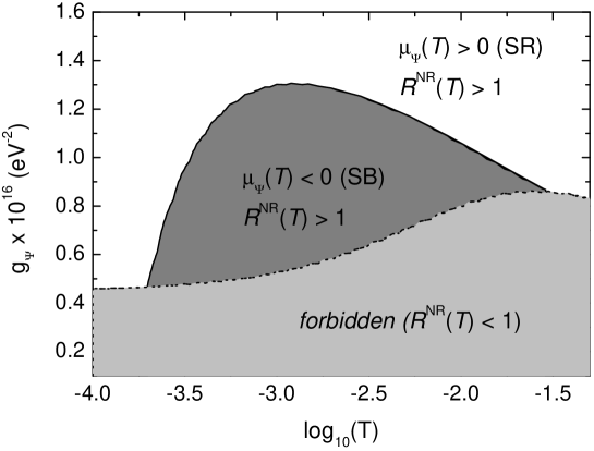
Figure 1: The phase diagram of the system in terms of $g_{\Psi}$ and temperature, for the parameters considered in the text. The dark gray region denotes a reentrant phase with symmetry breaking (SB) in the $\Psi$ direction, $\mu_{\Psi}(T)<0$. The region below it, in light gray, is the unstable region, $R^{\rm NR}(T)<1$ and above it is a symmetry restored (SR) phase, $\mu_{\Psi}(T)>1$. Temperature is given in units of eV.

Fig. 1 shows clearly the possibility of reentrant phases in the system, through an inverse symmetry breaking, in $\Psi$ direction. For instance, for $g_{\Psi}(T=0)=10^{-16}{\rm eV}^{-2}$, we find a reentrant symmetry broken phase starting at the temperature $T_{c,\Psi}^{\rm(ISB)}\simeq 3.4\times 10^{-4}{\rm eV}$ (or $\sim 4$ K) and ending at $T_{c,\Psi}^{\rm(SR)}\simeq 1.4\times 10^{-2}{\rm eV}$ (or $\sim 161$ K), through symmetry restoration. In this region of temperature and parameters, $R^{\rm NR}(T)>1$ and the (effective) potential is still bounded from below. In the $\Phi$ direction there is no symmetry breaking or reentrant phases at any temperature for the parameters considered.

3 Application to a Coupled Two-Species Dilute and Homogeneous Atomic Bose Gas Model

Let us now consider the case of model (1) as describing two coupled Bose gases of fixed densities $\rho_{\Phi}$ and $\rho_{\Psi}$, respectively. The model could then be describing a system composed by a mixture of coupled atomic gases, like the ones recently produced [8], with same chemical element in two different hyperfine states, or even two different mono-atomic Bose gases in the homogeneous case [9]. Here $\mu_{\Phi}$ and $\mu_{\Psi}$ are then explicitly chemical potentials added in the grand-canonical formalism to ensure the fixed densities for each Bose atom gas. Here we start describing the system in the broken phase in both $\Phi$ and $\Psi$ directions. Therefore, $\mu_{\Phi}\to-\mu_{\Phi}$ and $\mu_{\Psi}\to-\mu_{\Psi}$ in (1) and these chemical potentials are taken as positive quantities and with their values determined by the usual thermodynamic relation, in terms of the pressure $P(T,\mu_{\Phi},\mu_{\Psi})$,

$$\rho_{\Psi}=\frac{\partial P(T,\mu_{\Phi},\mu_{\Psi})}{\partial\mu_{\Psi}}\;,\;\;\;\;\rho_{\Phi}=\frac{\partial P(T,\mu_{\Phi},\mu_{\Psi})}{\partial\mu_{\Phi}}\;,$$ (2)

where the pressure is defined as the negative of the effective potential computed at its minima (which is the thermodynamic free energy of the system),

$$P\equiv P(T,\mu_{\Phi},\mu_{\Psi})=-V_{\rm eff}(T,\phi_{0},\psi_{0})\Bigr{|}_{\phi_{0}=\phi_{m},\psi_{0}=\psi_{m}}\;,$$ (3)

where $\phi_{m}$ and $\psi_{m}$ are the values of $\phi_{0}$ and $\psi_{0}$ that extremizes (corresponding to a minimum of) the effective potential,

$$\frac{\partial V_{\rm eff}(T,\phi_{0},\psi_{0})}{\partial\phi_{0}}\Bigr{|}_{\phi_{0}=\phi_{m},\psi_{0}=\psi_{m}}=0\;,\;\;\;\;\frac{\partial V_{\rm eff}(T,\phi_{0},\psi_{0})}{\partial\psi_{0}}\Bigr{|}_{\phi_{0}=\phi_{m},\psi_{0}=\psi_{m}}=0\;.$$ (4)

The effective potential follows from (1) by expanding the fields around the vacuum expectation values, $\langle\Phi\rangle=\phi_{0}/\sqrt{2}$ and $\langle\Psi\rangle=\psi_{0}/\sqrt{2}$, and it is evaluated in the one-loop approximation in a standard computation of quantum field theory at finite temperature (for the one-field case, see for instance [10]). At the tree-level, $\phi_{m}$ and $\psi_{m}$ are given in terms of the minima of the potential in (1),

$$\phi_{m}^{2}=6\frac{g_{\Psi}\mu_{\Phi}-3g\mu_{\Psi}}{g_{\Psi}g_{\Phi}-9g^{2}}\;,\;\;\;\psi_{m}^{2}=6\frac{g_{\Phi}\mu_{\Psi}-3g\mu_{\Phi}}{g_{\Psi}g_{\Phi}-9g^{2}}\;.$$ (5)

At finite temperature, the equations for $\phi_{m}$ and $\psi_{m}$ are given by analogous expressions to (5), but in terms of the effective chemical potentials instead, $\bar{\mu}_{\Phi}$ and $\bar{\mu}_{\Psi}$, that are defined by the solution of the self-consistent equations, $\bar{\mu}_{\Phi}=\mu_{\Phi}-\Sigma_{\phi,\phi}$ and $\bar{\mu}_{\Psi}=\mu_{\Psi}-\Sigma_{\psi,\psi}$, given in terms of the $\Phi$ and $\Psi$ field self-energies $\Sigma$.

The explicit expression for the pressure at finite temperature, obtained from the effective potential as described above and that follows from some length but straightforward calculation, is given by [11]

$$P(T,\mu_{\Phi},\mu_{\Psi}) = \frac{3}{2\left(g_{\Phi}g_{\Psi}-9g^{2}\right)}\left[g_{\Psi}\left(\mu_{\Phi}^{2}-\Sigma^{2}_{\phi,\phi}\right)+g_{\Phi}\left(\mu_{\Psi}^{2}-\Sigma^{2}_{\psi,\psi}\right)\right.$$ (6)

$$+ \left.6g\left(\Sigma_{\phi,\phi}\Sigma_{\psi,\psi}-\mu_{\Phi}\mu_{\Psi}\right)\right]-\int\frac{d^{3}{\bf q}}{(2\pi)^{3}}\left(\bar{A}_{+}+\bar{A}_{-}\right)\Bigr{|}_{{\lower 1.5pt\hbox{\tiny$\psi_{0}=\psi_{m}$}\above 0.0pt\raise 1.5pt\hbox{\tiny$\phi_{0}=\phi_{m}$}}}$$

$$- \frac{1}{\beta}\int\frac{d^{3}{\bf q}}{(2\pi)^{3}}\left[\ln\left(1-e^{-\beta\bar{A}_{+}}\right)+\ln\left(1-e^{-\beta\bar{A}_{-}}\right)\right]\Bigr{|}_{{\lower 1.5pt\hbox{\tiny$\psi_{0}=\psi_{m}$}\above 0.0pt\raise 1.5pt\hbox{\tiny$\phi_{0}=\phi_{m}$}}}\;,$$

where

$$\bar{A}_{\pm}^{2}=\frac{\bar{H}_{\Psi}\bar{G}_{\Psi}+\bar{H}_{\Phi}\bar{G}_{\Phi}}{2}\mp\frac{1}{2}\left[\left(\bar{H}_{\Psi}\bar{G}_{\Psi}-\bar{H}_{\Phi}\bar{G}_{\Phi}\right)^{2}+4g^{2}\psi_{m}^{2}\phi_{m}^{2}\bar{G}_{\Psi}\bar{G}_{\Phi}\right]^{1/2},$$ (7)

and

$$\bar{H}_{\Psi}\!\!=\!\!\frac{{\bf q}^{2}}{2m_{\Psi}}+\frac{g_{\Psi}}{3}\psi_{m}^{2}\;,\;\;\;\bar{G}_{\Psi}\!\!=\!\!\frac{{\bf q}^{2}}{2m_{\Psi}}\;,\;\;\;\bar{H}_{\Phi}\!\!=\!\!\frac{{\bf q}^{2}}{2m_{\Phi}}+\frac{g_{\Phi}}{3}\phi_{m}^{2}\;,\;\;\;\bar{G}_{\Phi}\!\!=\!\!\frac{{\bf q}^{2}}{2m_{\Phi}}\;.$$ (8)

$\bar{H}_{i}$ and $\bar{G}_{i}$ denote the Higgs and Goldstone modes, respectively, for each field in the broken phase.

From (2) and after some algebra to eliminate the dependence of these expressions on the chemical potentials, we find the expressions relating the total densities $\rho_{\Psi}$ and $\rho_{\Phi}$ with (the condensate densities) $\psi_{m}$ and $\phi_{m}$, as given by [11]

$$\rho_{\Psi}=\frac{\psi_{m}^{2}}{2}-\frac{1}{2}\int\frac{d^{3}{\bf q}}{(2\pi)^{3}}\left[\frac{\partial\bar{A}_{+}}{\partial\mu_{\Psi}}\left(1+2n_{\bar{A}_{+}}\right)+\frac{\partial\bar{A}_{-}}{\partial\mu_{\Psi}}\left(1+2n_{\bar{A}_{-}}\right)\right]\;,$$ (9)

and

$$\rho_{\Phi}=\frac{\phi_{m}^{2}}{2}-\frac{1}{2}\int\frac{d^{3}{\bf q}}{(2\pi)^{3}}\left[\frac{\partial\bar{A}_{+}}{\partial\mu_{\Phi}}\left(1+2n_{\bar{A}_{+}}\right)+\frac{\partial\bar{A}_{-}}{\partial\mu_{\Phi}}\left(1+2n_{\bar{A}_{-}}\right)\right]\;,$$ (10)

where $n_{\bar{A}_{\pm}}=1/[\exp(\beta A_{\pm})-1]$ and the partial derivatives of $\bar{A}_{\pm}$ with respect to $\mu_{\Phi}$ and $\mu_{\Psi}$ are defined by

$$\frac{\partial\bar{A}_{+}}{\partial\mu_{\Phi}}=-\frac{\left(\bar{H}_{\Phi}+\bar{G}_{\Phi}\right)}{4\bar{A}_{+}}\left[1+\frac{\left(\bar{H}_{\Psi}\bar{G}_{\Psi}-\bar{H}_{\Phi}\bar{G}_{\Phi}\right)-2g^{2}\phi_{m}^{2}\psi_{m}^{2}\bar{G}_{\Psi}}{\sqrt{\left(\bar{H}_{\Psi}\bar{G}_{\Psi}-\bar{H}_{\Phi}\bar{G}_{\Phi}\right)^{2}+4g^{2}\phi_{m}^{2}\psi_{m}^{2}\bar{G}_{\Phi}\bar{G}_{\Psi}}}\right],$$

$$\frac{\partial\bar{A}_{+}}{\partial\mu_{\Psi}}=-\frac{\left(\bar{H}_{\Psi}+\bar{G}_{\Psi}\right)}{4\bar{A}_{+}}\left[1-\frac{\left(\bar{H}_{\Psi}\bar{G}_{\Psi}-\bar{H}_{\Phi}\bar{G}_{\Phi}\right)+2g^{2}\phi_{m}^{2}\psi_{m}^{2}\bar{G}_{\Phi}}{\sqrt{\left(\bar{H}_{\Psi}\bar{G}_{\Psi}-\bar{H}_{\Phi}\bar{G}_{\Phi}\right)^{2}+4g^{2}\phi_{m}^{2}\psi_{m}^{2}\bar{G}_{\Phi}\bar{G}_{\Psi}}}\right],$$

$$\frac{\partial\bar{A}_{-}}{\partial\mu_{\Phi}}=-\frac{\left(\bar{H}_{\Phi}+\bar{G}_{\Phi}\right)}{4\bar{A}_{-}}\left[1-\frac{\left(\bar{H}_{\Psi}\bar{G}_{\Psi}-\bar{H}_{\Phi}\bar{G}_{\Phi}\right)-2g^{2}\phi_{m}^{2}\psi_{m}^{2}\bar{G}_{\Psi}}{\sqrt{\left(\bar{H}_{\Psi}\bar{G}_{\Psi}-\bar{H}_{\Phi}\bar{G}_{\Phi}\right)^{2}+4g^{2}\phi_{m}^{2}\psi_{m}^{2}\bar{G}_{\Phi}\bar{G}_{\Psi}}}\right],$$

$$\frac{\partial\bar{A}_{-}}{\partial\mu_{\Psi}}=-\frac{\left(\bar{H}_{\Psi}+\bar{G}_{\Psi}\right)}{4\bar{A}_{-}}\left[1+\frac{\left(\bar{H}_{\Psi}\bar{G}_{\Psi}-\bar{H}_{\Phi}\bar{G}_{\Phi}\right)+2g^{2}\phi_{m}^{2}\psi_{m}^{2}\bar{G}_{\Phi}}{\sqrt{\left(\bar{H}_{\Psi}\bar{G}_{\Psi}-\bar{H}_{\Phi}\bar{G}_{\Phi}\right)^{2}+4g^{2}\phi_{m}^{2}\psi_{m}^{2}\bar{G}_{\Phi}\bar{G}_{\Psi}}}\right].$$ (11)

The coupled equations (9) and (10) give completely the phase diagram for the condensates $\psi_{m}$ and $\phi_{m}$ as a function of the temperature and the densities. A qualitative analysis of the phase structure is also possible to be deduced already at this level from equations (9), (10) and (11). Note that for $g=0$, from (7) we obtain that $\bar{A}_{+}^{2}(g=0)=\bar{H}_{\Phi}\bar{G}_{\Phi}$, $\bar{A}_{-}^{2}(g=0)=\bar{H}_{\Psi}\bar{G}_{\Psi}$, and we obtain the Bogoliubov spectrum [6] for each field in the uncoupled case. Also, (9) and (10) decouples and we obtain as a result, for example for $\rho_{\Phi}$,

$$\rho_{\Phi}\!\!=\!\!\frac{\phi_{m}^{2}}{2}\!+\!\frac{1}{2}\!\int\frac{d^{3}{\bf q}}{(2\pi)^{3}}\frac{\frac{{\bf q}^{2}}{2m_{\Phi}}+\frac{g_{\Phi}\phi_{m}^{2}}{6}}{\sqrt{\frac{{\bf q}^{2}}{2m_{\Phi}}\left(\frac{{\bf q}^{2}}{2m_{\Phi}}+\frac{g_{\Phi}\phi_{m}^{2}}{3}\right)}}\!\!\left[\!1\!+\!\frac{2}{e^{\beta\sqrt{\frac{{\bf q}^{2}}{2m_{\Phi}}\left(\frac{{\bf q}^{2}}{2m_{\Phi}}+\frac{g_{\Phi}\phi_{m}^{2}}{3}\right)}}\!-1}\right],$$ (12)

with analogous equation for $\rho_{\Psi}$. Taking (12) at the critical point, $T=T_{c,\Phi}$, we have that $\phi_{m}(T=T_{c,\Phi})=0$, since the condensate density at $T_{c}$ vanishes and (12) gives $\rho_{\Phi}=\int d^{3}{\bf q}/(2\pi)^{3}[\exp\left({\bf q}^{2}/(2m_{\Phi}T_{c,\Phi})\right)-1]^{-1}$, or inverting it, $T_{c,\Phi}=2\pi/m_{\Phi}\left[\rho_{\Phi}/\zeta(3/2)\right]^{2/3}$, where $\zeta(3/2)\simeq 2.612$. This is the standard result for the critical temperature of an homogeneous ideal Bose gas. This result emerges because of the level of approximation we are considering. It is only modified by corrections due to the self-interactions through nonperturbative methods and it requires at least second order corrections in the self-energy (see, for instance, [12] and references therein).

Note also that, at the level of approximation we are considering, from the equations (7), (9), (10) and (11), if any of the fields go above the transition point (either $\phi_{m}=0$ or $\psi_{m}=0$) the two equations (9) and (10) also decouple, becoming independent of each other, since the cross-coupling term in (7) and (11) always appears multiplying both $\phi_{m}$ and $\psi_{m}$. As a result, no reentrant phase at high temperatures seems to be possible here. A computation performed in the restored phase case (similar to the one done in Sec. 2) also seems to confirm this result. This comes about as a consequence of the strong temperature dependence introduced by the chemical potentials through the relation (2) in both the broken and symmetric cases. In the broken (BEC) phase, it is also seen that the system exhibits a small dependence on the cross-coupling term (at one-loop order it is even insensitive to the sign of $g$). A throughout analysis of the phase structure coming from the coupled set of equations (9) and (10), including higher order terms, will be presented elsewhere [11].

References

References

- [1] Pinto M B and Ramos R O 2000 Phys. Rev. D61 125016 (Preprint hep-ph/9912273)
- [2] Pinto M B, Ramos R O and Parreira J E 2005 Phys. Rev. D 71 123519 (Preprint hep-th/0506131)
- [3] Pinto M B and Ramos R O 2006 J. Phys. A: Math. Gen. 39 6649 (Preprint cond-mat/0605508)
- [4] Goldenfeld N Lectures on Phase Transitions and The Renormalization Group, Frontiers in Physics, V. 85 (Addison-Wesley, NY, 1992)
- [5] Schupper N and Shnerb N M 2005 Phys. Rev. E 72 046107
- [6] Courteille Ph W, Bagnato V S and Yukalov V I 2001 Laser Phys. 11 659; Dalfovo F, Giorgini S, Pitaevskii L P and Stringari S 1999 Rev. Mod. Phys. 71 463
- [7] Gleiser M and Ramos R O 1993 Phys. Lett. B300 271 (Preprint hep-ph/9211219)
- [8] Myatt C J et al. 1997 Phys. Rev. Lett. 78 586; Matthews M R et al. 1998 Phys. Rev. Lett. 81 243
- [9] Pu H and Bigelow N P 1998 Phys. Rev. Lett. 80 1130; Ao P and Chui S T 1998 Phys. Rev. A 58 4836
- [10] Haugset T, Haugerud H and Ravndal F 1998 Ann. Phys. (N.Y.) 266 27
- [11] Pinto M B, Ramos R O and Souza Cruz F F, Preprint cond-mat/0606041
- [12] de Souza Cruz F F, Pinto M B, Ramos R O and Sena P 2002 Phys. Rev. A 65 053613 (Preprint cond-mat/0112306); Kneur J-L, Pinto M B and Ramos R O 2002 Phys. Rev. Lett. 89 210403 (Preprint cond-mat/0207089); 2003 Phys. Rev. A 68 043615 (Preprint cond-mat/0207295)