Non-Perturbative Renormalization Group calculation of the scalar self-energy

Abstract

We present the first numerical application of a method that we have recently proposed to solve the Non Perturbative Renormalization Group equations and obtain the $n$-point functions for arbitrary external momenta. This method leads to flow equations for the $n$-point functions which are also differential equations with respect to a constant background field. This makes them, a priori, difficult to solve. However, we demonstrate in this paper that, within a simple approximation which turns out to be quite accurate, the solution of these flow equations is not more complicated than that of the flow equations obtained in the derivative expansion. Thus, with a numerical effort comparable to that involved in the derivative expansion, we can get the full momentum dependence of the $n$-point functions. The method is applied, in its leading order, to the calculation of the self-energy in a 3-dimensional scalar field theory, at criticality. Accurate results are obtained over the entire range of momenta.

I Introduction

The non perturbative renormalization group (NPRG) Wetterich93 ; Ellwanger93 ; Tetradis94 ; Morris94 ; Morris94c stands out as a very promising formalism to address non perturbative problems, i.e., problems in which the absence of a small parameter prevents one to build a solution in terms of a systematic expansion. It leads to exact flow equations which are difficult to solve in general, but which offer the possibility for new approximation schemes. When only correlation functions at small momenta are needed, as is the case for instance in the calculation of critical exponents, a general approximation method to solve the infinite hierarchy of the NPRG equations has been developped Morris94c ; Bagnuls:2000ae ; Berges02 . This method, which can be systematically improved, is based on a derivative expansion of the the effective action. It has been applied successfully to a variety of physical problems, in condensed matter, particle or nuclear physics (for reviews, see e.g. Bagnuls:2000ae ; Berges02 ). However, in many situations, this is not enough: in order to calculate the quantities of physical interest, the knowledge of the full momentum dependence of the correlation functions is mandatory. Many efforts to get this information from the flow equations, involve truncations of various kinds truncation , following an early suggestion by Weinberg weinberg73 (see however Golner ; Parola ).

The present paper explores the applicability of the strategy that we proposed recently in Blaizot:2005xy , following our previous works Blaizot:2005wd ; Blaizot:2006vr in which we presented a scheme to obtain the momentum dependence of $n$-point functions from the flow equations. The strategy put forward in Blaizot:2005xy is based on the fact that the internal momentum $q$ in the integrals that determine the flow of the $n$-point functions is bounded by the regulator introduced by the NPRG. Since this regulator also guarantees that the vertex functions are smooth functions of the momenta, these can be expanded in powers of $q^{2}/\kappa^{2}$, $\kappa$ being the cut-off scale in the regulator. The “leading order” (LO) of the approximation scheme proposed in Blaizot:2005xy simply consists in keeping the lowest order of this expansion, i.e., in setting $q=0$ in the vertices. Doing so, and working in a constant external field, it is possible to relate to each other the various $n$-point functions that appear in a given flow equation through derivatives with respect to the external field, thereby closing the hierarchy of equations.

In Blaizot:2005xy we showed that the method reproduces perturbative results, at any desired order. Furthermore, we also showed that the LO is exact in the large $N$ limit of the $O(N)$ scalar model. Finally, one expects the method to provide, at each order of the expansion, results as good as those of the derivative expansion in the domain where the derivative expansion is valid.

The price to pay is that the resulting equations are also differential equations with respect to a uniform background field, with integral kernels that involve the solution itself. These integro-differential equations are a priori difficult to solve. The aim of this paper is to demonstrate that they can indeed be solved, with a numerical effort comparable to that involved in solving the flow equations that result from the derivative expansion, and to present a first application to the study of the 2-point correlation function of the scalar model, in the LO of the approximation scheme.

The outline of the paper is as follows. In section II we briefly recall some basic features of the NPRG and the essence of our approximation scheme in the case of a scalar field theory. In section III we analyze the structure of the flow equation for the 2-point correlation function and describe the strategy that we used to solve it. In section IV we present numerical results for the self-energy of the scalar field, at criticality and in $d=3$. The appendices gather technical material.

II The method

We consider a scalar field theory with the classical action

$$S=\int{\rm d}^{d}x\,\left\{{\frac{1}{2}}\left(\partial_{\mu}\varphi(x)\right)^{2}+\frac{r}{2}\,\varphi^{2}(x)+\frac{u}{4!}\,\varphi^{4}(x)\right\}\,.$$ (1)

The NPRG constructs a family of effective actions, $\Gamma_{\kappa}[\phi]$ (with $\phi$ the expectation value of the field in the presence of external sources), in which the magnitude of long wavelength fluctuations are controlled by an infrared regulator depending on a continuous parameter $\kappa$. The effective action $\Gamma_{\kappa}[\phi]$ interpolates between the classical action obtained for $\kappa=\Lambda$ (with $\Lambda$ the microscopic scale at which fluctuations are essentially suppressed), and the full effective action obtained when $\kappa\to 0$, i.e., when all fluctuations are taken into account (see e.g. Berges02 ). It is understood that the values of the parameters $r$ and $u$ of the classical action (1), as well as the field normalisation, are fixed at the microscopic scale $\Lambda$. One can write for $\Gamma_{\kappa}[\phi]$ an exact flow equation Tetradis94 ; Morris94 ; Morris94c :

$$\partial_{\kappa}\Gamma_{\kappa}[\phi]=\frac{1}{2}\int\frac{d^{d}q}{(2\pi)^{d}}(\partial_{\kappa}R_{\kappa}(q))\left[\Gamma_{\kappa}^{(2)}+R_{\kappa}\right]^{-1}_{q,-q},$$ (2)

where $\Gamma_{\kappa}^{(2)}$ is the second derivative of $\Gamma_{\kappa}$ with respect to $\phi$, and $R_{\kappa}$ denotes a family of “cut-off functions” depending on $\kappa$. There is a large freedom in the choice of $R_{\kappa}(q)$, abundantly discussed in the literature Ball95 ; Comellas98 ; Litim ; Canet02 . To be specific, in the present paper, we shall use for $R_{\kappa}(q)$ the following function Litim

$$R_{\kappa}(q)=Z_{\kappa}(\kappa^{2}-q^{2})\;\Theta(\kappa^{2}-q^{2}),$$ (3)

where $Z_{\kappa}$ is a function of $\kappa$ specified in the next section (see eq. (18)).

By deriving eq. (2) with respect to $\phi$, and then letting the field be constant, one gets the flow equation for the $n$-point functions $\Gamma^{(n)}$ in a constant background field $\phi$. More precisely, taking into account momentum conservation, one defines:

$$(2\pi)^{d}\;\delta^{(d)}\left(p_{1}+\cdots+p_{n}\right)\;\Gamma_{\kappa}^{(n)}(p_{1},\dots,p_{n};\phi)\qquad\qquad$$

$$\qquad\qquad=\int d^{d}x_{1}\dots\int d^{d}x_{n}e^{i\sum_{j=1}^{n}p_{j}x_{j}}\left.\frac{\delta^{n}\Gamma_{\kappa}}{\delta\phi(x_{1})\dots\delta\phi(x_{n})}\right|_{\phi(x)\equiv\phi}.$$ (4)

Then, the equation for the 2-point function reads:

$$\partial_{\kappa}\Gamma_{\kappa}^{(2)}(p;\phi) = \int\frac{d^{d}q}{(2\pi)^{d}}(\partial_{\kappa}R_{\kappa}(q))\left\{G_{\kappa}(q;\phi)\Gamma_{\kappa}^{(3)}(p,q,-p-q;\phi)\right.$$ (5)

$$\qquad\qquad\qquad\qquad\times G_{\kappa}(q+p;\phi)\Gamma_{\kappa}^{(3)}(-p,p+q,-q;\phi)G_{\kappa}(q;\phi)$$

$$\qquad\qquad\qquad\qquad\left.-\frac{1}{2}G_{\kappa}(q;\phi)\Gamma_{\kappa}^{(4)}(p,-p,q,-q;\phi)G_{\kappa}(q;\phi)\right\},$$

where

$$G^{-1}_{\kappa}(q;\phi)\equiv\Gamma^{(2)}_{\kappa}(q,-q;\phi)+R_{\kappa}(q),$$ (6)

and in eq. (5) we have used the simplified notation $\Gamma^{(2)}_{\kappa}(q;\phi)$ for $\Gamma^{(2)}_{\kappa}(q,-q;\phi)$, a notation that will be used throughout.

In general, the flow equation for a given $n$-point function involves the $m$-point functions with $m=n+1$ and $m=n+2$. Thus, the flow equations for the $n$-point functions do not close, but constitute an infinite hierarchy of coupled equations; this makes them difficult to solve.

In Blaizot:2005xy we proposed a method to solve this infinite hierarchy. It exploits the smoothness of the regularized $n$-point functions at small momenta, and the fact that the loop momentum $q$ in the right hand side of the flow equations (such as eq. (2) or eq. (5)) is limited to $q\mathrel{\hbox to0.0pt{\raise 2.20013pt\hbox{$<$}\hss}{\lower 2.20013pt\hbox{$\sim$}}}\kappa$ by the presence of the regulator $R_{\kappa}(q)$. The leading order (LO) of the method presented in Blaizot:2005xy thus consists in setting $q=0$ in the $n$-point functions in the r.h.s. of the flow equations, for instance

$$\Gamma^{(n)}_{\kappa}(p_{1},p_{2},...,p_{n-1}+q,p_{n}-q)\sim\Gamma^{(n)}_{\kappa}(p_{1},p_{2},...,p_{n-1},p_{n}).$$ (7)

Once this approximation is made, some momenta in some of the $n$-point functions vanish, and the corresponding $n$-point functions can be obtained as the derivatives of $m$-point functions ($m<n$) with respect to a constant background field, thereby allowing us to close the hierarchy of equations.

Specifically, in eq. (5) for the 2-point function, the 3- and 4-point functions in the r.h.s. will contain respectively one and two vanishing momenta after we set $q=0$. These can be related to the following derivatives of the 2-point function:

$$\Gamma_{\kappa}^{(3)}(p,-p,0;\phi)=\frac{\partial\Gamma_{\kappa}^{(2)}(p;\phi)}{\partial\phi},\hskip 28.45274pt\Gamma_{\kappa}^{(4)}(p,-p,0,0;\phi)=\frac{\partial^{2}\Gamma_{\kappa}^{(2)}(p;\phi)}{\partial\phi^{2}}.$$ (8)

One then arrives at a closed equation for $\Gamma_{\kappa}^{(2)}(p;\rho)$ (with $\rho\equiv\phi^{2}/2$):

$$\kappa\partial_{\kappa}\Gamma_{\kappa}^{(2)}(p;\rho)=J_{d}^{(3)}(p;\kappa;\rho)\;\left(\frac{\partial\Gamma_{\kappa}^{(2)}(p;\rho)}{\partial\phi}\right)^{2}-\frac{1}{2}I_{d}^{(2)}(\kappa;\rho)\;\frac{\partial^{2}\Gamma_{\kappa}^{(2)}(p;\rho)}{\partial\phi^{2}},$$ (9)

where

$$J_{d}^{(n)}(p;\kappa;\rho)\equiv\int\frac{d^{d}q}{(2\pi)^{d}}\kappa(\partial_{\kappa}R_{\kappa}(q))G_{\kappa}(p+q;\rho)G^{(n-1)}_{\kappa}(q;\rho),$$ (10)

and

$$I_{d}^{(n)}(\kappa;\rho)\equiv\int\frac{d^{d}q}{(2\pi)^{d}}\kappa(\partial_{\kappa}R_{\kappa}(q))G^{n}_{\kappa}(q;\rho).$$ (11)

Note that $J_{d}^{(n)}(p=0;\kappa;\rho)=I_{d}^{(n)}(\kappa;\rho)$.

At this point we note that the $n$-point functions at zero external momenta can all be considered as derivatives of a single function, the effective potential $V_{\kappa}(\rho)$. For instance,

$$\Gamma^{(2)}_{\kappa}(p=0;\rho)=\frac{\partial^{2}V_{\kappa}}{\partial\phi^{2}}.$$ (12)

The effective potential satisfies a flow equation which can be deduced from that for the effective action, eq. (2), when restricted to constant fields. It reads

$$\kappa\partial_{\kappa}V_{\kappa}(\rho)=\frac{1}{2}\int\frac{d^{d}q}{(2\pi)^{d}}\kappa(\partial_{\kappa}R_{\kappa}(q))G_{\kappa}(q;\rho).$$ (13)

The second derivative of this equation with respect to the background field yields a flow equation for $\Gamma^{(2)}_{\kappa}(p=0;\rho)$. Now, this equation does not coincide with eq. (9) in which we set $p=0$: indeed, in contrast to eq. (9), the vertices in the equation deduced from eq. (13) keep their $q$-dependence ($q$ being the loop momentum in eq. (13)). There is therefore an apparent inconsistency in our approximation scheme, that is however easily resolved by treating separately the zero momentum ($p=0$) and the non-zero momentum ($p\neq 0$) sectors. In fact, in doing so, we get more accuracy in the sector $p=0$ than in the sector $p\neq 0$.

Let us then write :

$$\Gamma^{(2)}_{\kappa}(p;\rho)=p^{2}+\frac{\partial^{2}V_{\kappa}}{\partial\phi^{2}}+\Sigma_{\kappa}(p;\rho),$$ (14)

where

$$\Sigma_{\kappa}(p;\rho)\equiv\Gamma^{(2)}_{\kappa}(p;\rho)-p^{2}-\Gamma^{(2)}_{\kappa}(p=0;\rho).$$ (15)

We shall refer to $\Sigma_{\kappa}(p;\rho)$ as the self-energy (although it differs from the usual self-energy by the subtraction of the momentum independent contribution $\Gamma^{(2)}_{\kappa}(p=0;\rho)$). By definition, $\Sigma_{\kappa}(p=0;\rho)=0$, and at criticality, $\Gamma^{(2)}_{\kappa=0}(p=0;\rho)=0$. We then proceed with separate approximations in the two sectors with $p=0$ and $p\neq 0$.

In the sector $p\neq 0$, it is $\Sigma_{\kappa}(p;\rho)$, rather than $\Gamma^{(2)}_{\kappa}(p;\rho)$ which satisfies the approximate eq. (9) (strictly speaking, eq. (9) to which one subtracts the same equation with $p=0$):

$$\kappa\partial_{\kappa}\Sigma(p;\rho)=\left[J_{d}^{(3)}(p;\kappa;\rho)\;\left(\frac{\partial\Gamma_{\kappa}^{(2)}(p;\rho)}{\partial\phi}\right)^{2}-\frac{1}{2}I_{d}^{(2)}(\kappa;\rho)\;\frac{\partial^{2}\Gamma_{\kappa}^{(2)}(p;\rho)}{\partial\phi^{2}}\right]-[p\to 0].$$ (16)

Eq. (16) is the flow equation for the momentum dependent part of the 2-point function at LO of our approximation scheme. It is a partial differential equation with respect to the two real variables, $\kappa$ and $\rho$, with the momentum $p$ playing the role of a parameter. It is to be integrated from $\kappa=\Lambda$, with initial condition $\Sigma_{\Lambda}(p;\rho)=0$ (see eqs. (1) and (15)), to $\kappa=0$ where it yields the physical self-energy $\Sigma(p;\rho)\equiv\Sigma_{\kappa=0}(p;\rho)$.

Eq. (16) is to be solved together with the equation in the sector $p=0$, i.e., with the equation for the effective potential, with initial condition $V_{\Lambda}(\rho)=r\rho+(u/6)\rho^{2}$ (see eq. (1)). In eq. (13) for $V_{\kappa}(\rho)$, we use the propagator (14) in which $\Sigma_{\kappa}(p;\rho)$ is solution of eq. (16) and $\Gamma^{(2)}_{\kappa}(q=0;\rho)$ is determined self-consistently from the effective potential, using eq. (12).

It is not difficult to verify that (in the perturbative regime) this scheme has 2-loop accuracy for the effective potential, and only one-loop accuracy for the self-energy. Besides, in the low momentum region it is as accurate as the derivative expansion at next-to-leading order.

III Analysis of the flow equation

There are two features of eq. (16) that make it a priori difficult to solve. First, the two functions $J_{d}^{(3)}(p;\kappa;\rho)$ and $I_{d}^{(2)}(\kappa;\rho)$, are functionals of the solution $\Gamma^{(2)}_{\kappa}(p;\rho)$ (see eq. (6)). Second the different values of $p$ are coupled through the propagator $G_{\kappa}(p+q)$ entering the calculation of $J^{(3)}_{d}(p;\kappa;\rho)$. In principle, one should therefore solve eq. (16) self-consistently, and simultaneously for all values of $p$. However, in this section, we shall show that it is possible to make an accurate calculation of $J^{(3)}_{d}(p;\kappa;\rho)$ and $I_{d}^{(2)}(\kappa;\rho)$ using approximate propagators. This yields an approximate version of eq. (16) that can be solved for each given value of $p$. The validity of this approximation will be checked in the next section.

Consider first the function $I_{d}^{(n)}(\kappa;\rho)$, which does not depend on $p$. The smoothness of the $n$-point functions and the fact that $q\leq\kappa$, suggest to perform in the propagators of the right-hand-side of eq. (11) an approximation similar to that applied to the other $n$-point functions, i.e., set $q=0$. However, in order to maintain the exact one-loop properties of the flow equations, one cannot simply set $q=0$ in the propagators: rather, one needs to keep a momentum dependence close to that of the free propagators. Thus, we shall use for the propagators entering the calculation of $I^{(n)}_{d}(\kappa;\rho)$ the following approximate form

$$G_{\kappa}^{-1}(q;\rho)\approx Z_{\kappa}q^{2}+\Gamma_{\kappa}^{(2)}(q=0;\rho)+R_{\kappa}(q),$$ (17)

where

$$Z_{\kappa}\equiv\left.{\frac{\partial\Gamma_{\kappa}^{(2)}}{\partial q^{2}}}\right|_{q=0,\rho=\rho_{0}}.$$ (18)

As well known Morris94c , and will be verified in app. A, $\left.\partial\Gamma^{(2)}(q;\rho)/\partial q^{2}\right|_{q=0}$ depends weakly on $\rho$. Accordingly, one expects $Z_{\kappa}$ to depend weakly on the value chosen for $\rho_{0}$. As will be seen in app. A, the choice $\rho_{0}=0$ is here the simplest. With the propagator (17), and the function (3) for $R_{\kappa}(q)$ one can calculate $I_{d}^{(n)}(\kappa;\rho)$ analytically:

$$I_{d}^{(n)}(\kappa;\rho)=2K_{d}\frac{\kappa^{d+2-2n}}{Z_{\kappa}^{n-1}}\frac{1}{(1+\hat{m}^{2}_{\kappa}(\rho))^{n}}\left(1-\frac{\eta_{\kappa}}{d+2}\right).$$ (19)

In this expression,

$$\eta_{\kappa}\equiv-\kappa\partial_{\kappa}\ln Z_{\kappa}$$ (20)

is the running anomalous dimension and

$$\hat{m}^{2}_{\kappa}(\rho)\equiv\frac{\Gamma_{\kappa}^{(2)}(q=0;\rho)}{\kappa^{2}Z_{\kappa}},$$ (21)

is a dimensionless, field-dependent, effective mass. $K_{d}$ is a number resulting from angular integration, $K_{d}^{-1}\equiv d\;2^{d-1}\;\pi^{d/2}\;\Gamma(d/2)$ (e.g., $K_{3}=1/(6\pi^{2})$). Notice that, for $d>2$, $I_{d}^{(2)}(\kappa;\rho)\to 0$ when $\kappa\to 0$.

We shall calculate the function $J^{(3)}_{d}(p,\kappa;\rho)$ in a similar way, arguing that in this calculation one can assume $p\mathrel{\hbox to0.0pt{\raise 2.20013pt\hbox{$<$}\hss}{\lower 2.20013pt\hbox{$\sim$}}}\kappa$ : the propagator $G_{\kappa}(p+q;\rho)$ in eq. (10) is small as soon as $p/\kappa$ is large, and one can indeed verify that the function $J^{(3)}_{d}(p;\kappa;\rho)$ vanishes approximately as $\kappa^{2}/p^{2}$ for large values of $p/\kappa$ (see the explicit expressions (B) and (B) given in app. B). Thus, in the region where $J^{(3)}_{d}(p;\kappa;\rho)$ has a significant value, one can use for $G_{\kappa}(p+q;\rho)$ an expression similar to (17), namely

$$G_{\kappa}^{-1}(p+q;\rho)\approx Z_{\kappa}(p+q)^{2}+\Gamma^{(2)}_{\kappa}(0;\rho)+R_{\kappa}(p+q).$$ (22)

One can then calculate the function $J^{(3)}_{d}(p;\kappa;\rho)$ analytically (in $d=3$). The resulting expression is more complicated than that of $I_{d}^{(2)}(\kappa;\rho)$, eq. (19). It is given in app. B (see also Blaizot:2006vr ). Observe that the regulator in eq. (3) is not analytic at $q\sim\kappa$. This generates non analyticities in $J^{(3)}_{d}(p;\kappa;\rho)$; but these occur only in the third derivative with respect to $p$, at $p=0$ and at $p=2\kappa$ (cf. the odd powers of $\bar{p}$ in eqs. (B-43)), and they play no role at the present level of approximation.

With the approximations just discussed, $I_{d}^{(2)}(\kappa;\rho)$ and $J^{(3)}_{d}(p;\kappa;\rho)$ depend only on quantities that enter the flow equations at $p=0$, namely $\hat{m}^{2}_{\kappa}(\rho)$ and $Z_{\kappa}$ (or $\eta_{\kappa}$). As we discuss in app. A, these quantities can be obtained from a modified version of the Local Potential approximation Berges02 that we call the LPA’. The strategy to solve eq. (16) consists then in two steps: one first solves the LPA’ to get $\hat{m}^{2}_{\kappa}(\rho)$ and $\eta_{\kappa}$; then, for each value of $p$, one solves eq. (16) with the kernels $I_{d}^{(2)}(\kappa;\rho)$ and $J_{d}^{(3)}(p;\kappa;\rho)$ that are calculated with $\hat{m}^{2}_{\kappa}(\rho)$, $Z_{\kappa}$ and $\eta_{\kappa}$ determined from the LPA’.

Note that, generally, the flow of $\Sigma$ gets strongly suppressed below some non vanishing value of $\kappa$. In $d=3$, this can be inferred from the properties of the functions $I_{3}^{(2)}(\kappa;\rho)$ and $J_{3}^{(3)}(p;\kappa;\rho)$ discussed above, and it will be verified explicitly on the numerical results presented in the next section (see Fig. 1). In fact, the flow of $\Sigma$ receives two contributions: the first involves the external momentum $p\neq 0$ and is suppressed when $\kappa\mathrel{\hbox to0.0pt{\raise 2.20013pt\hbox{$<$}\hss}{\lower 2.20013pt\hbox{$\sim$}}}p$ ($J_{3}^{(3)}(p;\kappa;\rho)$ vanishes rapidly when $\kappa$ becomes smaller than $p$, while $I_{3}^{(2)}(\kappa;\rho)\sim\kappa$); the other contribution is independent of $p$ and, at criticality, is suppressed for $\kappa\mathrel{\hbox to0.0pt{\raise 2.20013pt\hbox{$<$}\hss}{\lower 2.20013pt\hbox{$\sim$}}}\kappa_{c}\sim u/10$ (see app. A, and in particular fig. 6). Accordingly, one expects the flow to stop when $\kappa$ reaches the smallest of $\kappa_{c}$ and $p$.

The function $\Gamma_{\kappa}^{(2)}(p;\rho)$ exhibits a simple scaling behavior. Consider for simplicity the zero field case $\rho=0$, and the ratio

$$\frac{p^{2}+\Gamma_{\kappa}^{(2)}(0;\rho=0)+\Sigma_{\kappa}(p;\rho=0)}{\Gamma_{\kappa}^{(2)}(0;\rho=0)}=f\left(\frac{p}{\kappa},\frac{p}{u}\right).$$ (23)

At criticality, and in the scaling regime where $p,\kappa\ll u$, we expect $f$ to become independent of $u$, and therefore a function of $p/\kappa$ only. As will be shown in the next section, the solution of eq. (16) verifies this property. Note that this scaling behavior is reproduced only when including a renormalization factor $Z_{\kappa}$ whose flow is determined consistently from that of ${\partial\Sigma_{\kappa}}/{\partial p^{2}}$ for $p<\kappa$, as obtained from eq. (16). This calculation of $Z_{\kappa}$ is explained in app. A. We have tested the consequence of setting $Z_{\kappa}=1$ in the propagators (17) and (22), corresponding to the Local Potential approximation (as opposed to the LPA’). Doing so does not alter the self-energy in any significant way when $p\mathrel{\hbox to0.0pt{\raise 2.20013pt\hbox{$>$}\hss}{\lower 2.20013pt\hbox{$\sim$}}}u$, but in the IR regime, the scaling behavior is only approximate.

IV Numerical results and discussion

We now turn to the numerical solution of the flow equation for $\Sigma_{\kappa}(p;\rho)$, at $d=3$ and at criticality. Our goal is to assess the quality of the approximation scheme, and there are two aspects that we shall examine. First, since the strategy described in the previous section provides only an approximate solution to eq. (16), we shall estimate by how much this approximate solution differs from the exact solution of this equation. Second, since eq. (16) itself is only the LO approximation of the method described in Blaizot:2005xy , we shall compare our results with known ones concerning the self-energy of the scalar model at criticality.

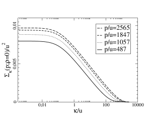
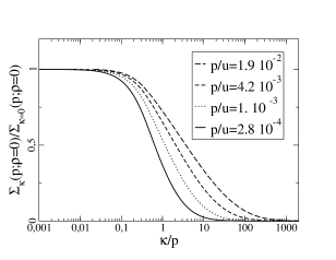
Figure 1: Left: $\Sigma_{\kappa}(p;\rho=0)/u^{2}$ as a function of $\kappa/u$ for various values of $p\gg u$. The flow stops at $\kappa\mathrel{\hbox to0.0pt{\raise 2.20013pt\hbox{$<$}\hss}{\lower 2.20013pt\hbox{$\sim$}}}\kappa_{c}\sim u/10$. Right: $\Sigma_{\kappa}(p;\rho=0)/\Sigma_{\kappa=0}(p;\rho=0)$ as a function of $\kappa/p$ for various values of $p\ll u$. The flow stops at $\kappa\mathrel{\hbox to0.0pt{\raise 2.20013pt\hbox{$<$}\hss}{\lower 2.20013pt\hbox{$\sim$}}}p/10$.

Let us start by considering general properties of the flow, and verify in particular that it essentially stops for a small value of $\kappa$. Fig. 1 displays the self-energy, $\Sigma_{\kappa}(p;\rho=0)$ as a function of $\kappa/u$, for different values of $p$. Calculations are made for $u/\Lambda=3.54\times 10^{-4}$ (this value is small enough to guarantee that the results are independent of $\Lambda$). The left panel of fig. 1 shows the flow of $\Sigma_{\kappa}(p;\rho=0)$ for values of $p$ in the UV regime, i.e., $p\gg\kappa_{c}\sim u/10$; for all the considered values of $p$ the flow stops at $\kappa_{c}$. The right panel of fig. 1 presents the flow of the self-energy when $p$ is in the IR regime, i.e., when $p\ll\kappa_{c}$. In this case, we have divided $\Sigma_{\kappa}(p;\rho=0)$ by its physical value $\Sigma(p;\rho=0)\equiv\Sigma_{\kappa=0}(p;\rho=0)$, in order to make it more obvious that the flow only stops when $\kappa\mathrel{\hbox to0.0pt{\raise 2.20013pt\hbox{$<$}\hss}{\lower 2.20013pt\hbox{$\sim$}}}p/10$.

We now turn to the physical self-energy $\Sigma(p)\equiv\Sigma_{\kappa=0}(p;\rho=0)$ in vanishing external field, displayed in fig. 2 as a function of $p/u$, and discuss its behavior in the various momentum regions: $p\gg u$, $p\ll u$, $p\sim\kappa_{c}\sim u/10$. We have checked that the curve in fig. 2, i.e., $(1/u^{2})\Sigma(p/u)$, is “universal”, i.e., independent of $u$ and $\Lambda$, provided $u/\Lambda$ is small enough.

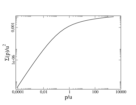
Figure 2: $\Sigma(p)/u^{2}$, in $d=3$, at criticality and zero external field, as a function of $p/u$.

In the perturbative regime ($p\gg u$), one expects $\Sigma(p)\approx(u^{2}/96\pi^{2})\log(p/u)$. In app. C we show that the analytical solution of eq. (16) preserves this behavior, although the coefficient in front of the logarithm is $(u^{2}/9\pi^{4})$, 8% larger (the LO approximation does not include all the 2-loop perturbative diagrams exactly). Our approximate numerical solution reproduces this result. As explained in Blaizot:2005xy , at the NLO of our approximation scheme, which is beyond the scope of the present paper, the contribution of the 2-loops diagrams would be exactly included and the correct prefactor $(u^{2}/96\pi^{2})$ would be recovered.

In the IR region ($p\ll u$) we expect the self-energy to behave as

$$p^{2}+\Sigma(p)=Ap^{2-\eta^{*}},$$ (24)

where $\eta^{*}$ is the anomalous dimension. By analyzing the small momentum behavior of $\Sigma(p)$, we get numerically $\eta^{*}=0.05218$. An alternative way to determine $\eta^{*}$ is to extract it from the $\kappa$ dependence of $Z_{\kappa}$ (see eq. (20)). As recalled in app. A, in the critical regime, i.e., when $\kappa\mathrel{\hbox to0.0pt{\raise 2.20013pt\hbox{$<$}\hss}{\lower 2.20013pt\hbox{$\sim$}}}\kappa_{c}$, $Z_{\kappa}\propto\kappa^{-\eta^{*}}$, with $\eta^{*}=0.05220$ the fixed point value of $\eta_{\kappa}$ (see fig. 6). It is also shown in fig. 6 in app. A that the quantity $\Gamma^{(2)}_{\kappa}(p=0;\rho=0)/(\kappa^{2}Z_{\kappa})$ goes to a fixed point, which confirms the behavior of $\Gamma^{(2)}_{\kappa}(p=0;\rho=0)\sim\kappa^{2-\eta}$ expected in the scaling regime.

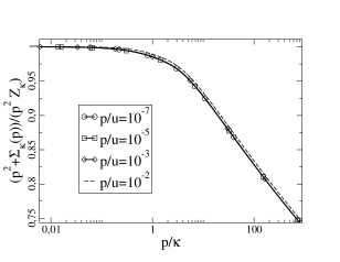
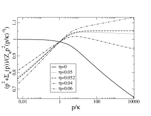
Figure 3: The ratio ${(p^{2}+\Sigma_{\kappa}(p))}/({Z_{\kappa}p^{2}})$ as a functio of $p/\kappa$. Right: the same ratio divided by $(p/\kappa)^{-\eta^{*}}$.

We have performed a more stringent test of scaling by studying the function ${(p^{2}+\Sigma_{\kappa}(p))}/({Z_{\kappa}p^{2}})$. This function is displayed in fig. 3 as a function of $p/\kappa$. By definition of $Z_{\kappa}$ (see eq. (18)), when $\kappa$ is kept fixed and $p\to 0$, this function goes to one. Furthermore, as explained before, in the scaling regime $p,\kappa\ll u$, one expects this function to depend on $p/\kappa$ only, which is indeed well verified, as can be seen on the left panel of fig. 3; it is only for values of $p$ which are not small enough ($p/u=10^{-2}$, corresponding to the dashed line) that violation of this scaling starts to become significant. Moreover, as can be seen on the figure, $p^{2}+\Sigma_{\kappa}(p)$ is well approximated by $Z_{\kappa}p^{2}$ for all $p\mathrel{\hbox to0.0pt{\raise 2.20013pt\hbox{$<$}\hss}{\lower 2.20013pt\hbox{$\sim$}}}\kappa$. In the right panel of fig. 3, we have plotted the ratio ${(p^{2}+\Sigma_{\kappa}(p))}/({Z_{\kappa}p^{2}})$ divided by $(p/\kappa)^{-\eta^{*}}$. Recall that when $\kappa\ll p\ll\kappa_{c}$, one expects $p^{2}+\Sigma_{\kappa}(p)\sim p^{2-\eta^{*}}$, while $Z_{\kappa}\sim\kappa^{-\eta^{*}}$ when $\kappa\mathrel{\hbox to0.0pt{\raise 2.20013pt\hbox{$<$}\hss}{\lower 2.20013pt\hbox{$\sim$}}}\kappa_{c}$. Therefore when $1\ll p/\kappa\ll\kappa_{c}/\kappa$, one expects ${(p^{2}+\Sigma_{\kappa}(p))}/({Z_{\kappa}p^{2}})\sim(p/\kappa)^{-\eta^{*}}$, so that the quantity which is plotted should be constant. As seen in the right panel of fig. 3, this is indeed the case for the value $\eta^{*}=0.05219$, which confirms the coherence of the whole calculation.

Our estimate for the anomalous dimension, $\eta^{*}\approx 0.052$ is to be compared with the results $\eta^{*}=0$, $\eta^{*}=0.044$ and $\eta^{*}=0.033$ obtained with the derivative expansion at LO, NLO and NNLO, respectively Morris94c ; Canet02 ; Canet03 , and $\eta^{*}=0.0335\pm 0.0025$ from the resummed 7 loop calculation of ref.  refeta . Thus, the LO of our approximation scheme yields a result slightly larger that the NLO of the derivative expansion. The value of $\eta^{*}$ obtained here is also slightly larger than that obtained in Blaizot:2005wd using a different version of the LPA’ than that used here. In fact, the deviation of the present estimate of $\eta^{*}$ from the value $0.044$ obtained with the derivative expansion in next-to-leading order can be taken as a measure of the error introduced, in the scaling regime, by our use of the LPA’ in our approximate solution of eq. (16): as already mentioned, if we had solved eq. (16) exactly, one should have obtained essentially the same value as in the derivative expansion at NLO.

We turn now to the intermediate momentum region, which we shall probe with a quantity which is very sensitive to the cross-over between the two regimes just studied:

$$\Delta\langle\phi^{2}\rangle=\int\frac{d^{3}p}{(2\pi)^{3}}\,\left(\frac{1}{p^{2}+\Sigma(p)}-\frac{1}{p^{2}}\right).$$ (25)

As shown for instance in Blaizot:2004qa , the integrand in eq. (25) is peaked at $p\sim\kappa_{c}$ (in fact it takes significant values only in the region $10^{-3}\mathrel{\hbox to0.0pt{\raise 2.20013pt\hbox{$<$}\hss}{\lower 2.20013pt\hbox{$\sim$}}}p/u\mathrel{\hbox to0.0pt{\raise 2.20013pt\hbox{$<$}\hss}{\lower 2.20013pt\hbox{$\sim$}}}10$). This quantity has been much studied recently for a scalar model with $O(2)$ symmetry because it determines then the shift of the critical temperature of the weakly repulsive Bose gas club . For the simple scalar model studied in this paper, lattice calculations measure latt3 $\Delta\langle\phi^{2}\rangle/u=-(4.95\pm 0.41)\times 10^{-4}$ while the “7 loop” resummed calculation of ref. Kastening:2003iu yields $\Delta\langle\phi^{2}\rangle/u=-(4.86\pm 0.45)\times 10^{-4}$. With the present numerical solution, one gets $\Delta\langle\phi^{2}\rangle/u=-5.39\times 10^{-4}$. This is only slightly larger than the value $\Delta\langle\phi^{2}\rangle/u=-5.03\times 10^{-4}$ obtained in the next-to-leading order of the scheme presented in Blaizot:2005wd ; Blaizot:2006vr .

We conclude that with the LO of the present approximation scheme, we obtain an accurate description of the self-energy in the entire range of momenta. Since we have solved only appproximately eq. (16), it remains to study by how much the solution that we have obtained differs from the exact solution of eq. (16). We have already indications about the accuracy of the approximation both in the UV and in the IR. In the UV, we reproduce the expected result (which differs by 8% from the exact 2-loop result). We also loose the 2-loop accuracy with which the efffective potential could be obtained in the LO of our scheme, by using LPA’ propagators. In the IR, we have seen that the result that we got for the anomalous dimension is 0.052 instead of a value close to 0.044 that would have been obtained had we solved exactly eq. (16). As a further test, we have recalculated $I^{(2)}_{3}(\kappa;\rho)$ and $J_{3}^{(3)}(p;\kappa;\rho)$ using, instead of the LPA’ propagators, the propagators (6) in which $\Gamma^{(2)}_{\kappa}(p;\rho)$ is the 2-point function that has been obtained in this section by approximately solving eq. (16).

In fig. 4 we plot the ratio of the function $I^{(2)}_{3}(\kappa;\tilde{\rho})$ ($\tilde{\rho}\sim\rho/\kappa$, see. eq. (32)) calculated with the propagator obtained from the numerical integration of the flow equation divided by the function given by eq. (19). One can see that the smaller the value of $\kappa$, the larger the difference, and that the main error is for values of $\tilde{\rho}$ around the minimum $\tilde{\rho}_{min}$ of the effective potential ($\tilde{\rho}_{min}$ goes from 1.8 to 3 as $\kappa$ runs from $\Lambda$ to 0). Nevertheless, the difference stabilizes for small enough $\kappa$ and it never exceeds 4%. The right panel of fig. 4 shows the comparison of the two curves in the worst situation, i.e., for small values of $\kappa$, as a function of $\tilde{\rho}$: the curves are hardly distinguishable.

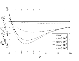
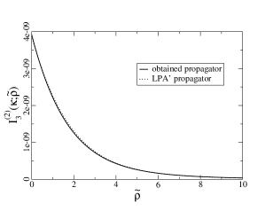
Figure 4: Left: The ratio of the function $I_{3}^{(2)}(\kappa;\tilde{\rho})$ calculated with the obtained numerical propagator and with the approximate LPA’ propagator (as explained in the text), as a function of $\tilde{\rho}$, for different values of $\kappa/u$. Right: The function $I_{3}^{(2)}(\kappa;\tilde{\rho})$ as a function of $\tilde{\rho}$, for $\kappa/u=3\times 10^{-4}$, calculated with the approximate propagator (dotted line) and with the obtained numerical propagator (solid line).

The same analysis is repeated for $J_{3}^{(3)}$. Again, it is only for small values of $\kappa$ that the two functions differs. In the left panel of fig. 5 we display the ratio of the function $J_{3}^{(3)}$ calculated respectively with the obtained (numerator) and the approximate LPA’ (denominator) propagators, for $\kappa/u=3\times 10^{-4}$, for various values of $\tilde{\rho}$. The difference can be large, but only in the region ($p\gg\kappa$) where the function $J_{3}^{(3)}$ itself is very small. In the region where the function is non negligeable, the difference between the two calculations never exceeds 5%. As was the case for $I_{3}^{(2)}$, the largest error occurs for values of $\tilde{\rho}$ near the minumum of the potential. In the right panel of fig. 5, we plot the two functions for the same values of $\kappa$ and $\tilde{\rho}$ as in the left panel: the difference between the two calculations of $J_{3}^{(3)}$ is invisible on such a plot.

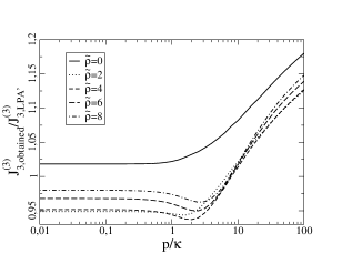
Figure 5: Left: The ratio of the function $J^{(3)}_{3}(p;\kappa;\tilde{\rho})$ calculated with the obtained numerical propagator and with the approximate LPA’ propagators, as a function of $p/\kappa$, for $\kappa/u=3\times 10^{-4}$ and for different values of $\tilde{\rho}$. Right: The function $J^{(3)}_{3}(p;\kappa;\tilde{\rho})/J^{(3)}_{3}(p=0;\kappa;\tilde{\rho})$ calculated with the obtained numerical propagator compared to that calculated with the approximate propagators, as a function of $p/\kappa$, for $\kappa/u=3\times 10^{-4}$ and for different values of $\tilde{\rho}$.

V Conclusions and perspectives

We have demonstrated in this paper that the method proposed in Blaizot:2005xy allows for concrete numerical applications. We have calculated the self-energy of the scalar model, at the LO of the approximation scheme, at criticality, at zero external field, in $d=3$, and have obtained accurate results over the whole range of momenta. Already at this level of approximation the results obtained compare well with those of more elaborate techniques. Worth emphasizing is the fact that the scaling behavior of the self-energy is accurately reproduced: not only do we get a reasonable estimate of the anomalous dimension, but the entire dependence of the self- energy on the momentum and the cut-off follows accurately the expected scaling behavior. To our knowledge, this is the first time that an approximate solution of the NPRG flow equations is constructed with these properties.

In the present paper, whose main objective was to confirm the applicability of the method to a concrete calculation, we solved approximately the flow equation (16). However, several tests suggest that this approximate solution differs in fact very little from the complete solution of (16). Of course, a definite statement concerning the error made in the present calculation can only come from a comparison with the exact solution. This, we believe, is within reach. Similarly, work is in progress to test the convergence of the procedure by calculating the next-to-leading order contribution.

The method of ref. Blaizot:2005xy builds on our previous works on the same subject Blaizot:2005wd ; Blaizot:2006vr . The results presented in this paper indicate that it is both conceptually simpler, and numerically more accurate, than the method which we have developed in Blaizot:2005wd ; Blaizot:2006vr . It offers the possibility of applications to a variety of non-perturbative problems, where the knowledge of the momentum dependence of $n$-point functions is necessary. Even the approximate treatment presented in this paper could constitute an interesting starting point in situations where only a semi-quantitative description would be valuable.

Appendix A The $p=0$ sector

As discussed in the main text, our approximate solution of eq. (16) builds on the prior determination of quantities that are independent of momentum. These are calculated using a variant of the derivative expansion that we describe in this appendix. The derivative expansion is usually Berges02 formulated in terms of an ansatz for the running effective action $\Gamma_{\kappa}[\phi]$, including terms up to a given number of derivatives of the field. Its leading order, the so-called local potential approximation (LPA), assumes that the effective action has the form:

$$\Gamma_{\kappa}^{LPA}[\phi]=\int d^{d}x\left\{\frac{1}{2}\partial_{\mu}\phi_{a}\partial_{\mu}\phi_{a}+V_{\kappa}(\rho)\right\}.$$ (26)

where the derivative term is simply the one appearing in the classical action, and $V_{\kappa}(\rho)$ is the effective potential. In the next-to-leading order (NLO), one assumes Wetterich93

$$\Gamma^{NLO}_{\kappa}[\phi]=\int d^{d}x\left\{\frac{Z_{\kappa}(\rho)}{2}\partial_{\mu}\phi_{a}\partial_{\mu}\phi_{a}+V_{\kappa}(\rho)\right\}.$$ (27)

An interesting improvement of the LPA, which we refer to as the LPA’, is a simplified version of the NLO that consists in ignoring the $\rho$-dependence of $Z_{\kappa}(\rho)$, i.e., in chosing $Z_{\kappa}=Z_{\kappa}(\rho_{0})$ where $\rho_{0}$ is a given value of $\rho$, usually taken to be the running minimum of the potential. In the LPA’ one solves simultaneously the flow equations for both the effective potential $V_{\kappa}(\rho)$ (a partial differential equation in $\kappa$ and $\rho$) and for $Z_{\kappa}$. In this approximation, the inverse propagator takes the form of eq. (17): $G^{-1}_{\kappa}(q^{2};\phi)={Z_{\kappa}q^{2}+V_{\kappa}^{\prime\prime}(\phi)+R_{\kappa}(q)},$ with $V_{\kappa}^{\prime\prime}(\phi)=d^{2}V_{\kappa}/d\phi^{2}$. The LPA’ allows for a non-trivial anomalous dimension, which is determined from the cut-off dependence of $Z_{\kappa}$ (see eq. (20) and ref. Wetterich93 ).

The procedure followed in this paper to determine the field renormalisation constant $Z_{\kappa}$ differs slightly from that used in Blaizot:2005wd . This is because, as explained in sect. III, we need the calculation of $Z_{\kappa}$ to be consistent with the approximate eq. (16) for the 2-point function. This is essential to get the proper scaling behavior of $\Gamma^{(2)}_{\kappa}(p;\rho)$ at small momenta. We set:

$$Z_{\kappa}(\rho)\equiv 1+\left.\frac{\partial\Sigma_{\kappa}(p;\rho)}{\partial p^{2}}\right|_{p=0},$$ (28)

where $\Sigma_{\kappa}(p;\rho)$ is defined in eq. (15). Notice that, using eq. (18), $Z_{\kappa}(\rho_{0})=Z_{\kappa}$. The flow equation obeyed by $Z_{\kappa}(\rho)$ reads

$$\kappa\partial_{\kappa}Z_{\kappa}(\rho)=\left.\frac{\partial J_{d}^{(3)}(p^{2},\rho)}{\partial p^{2}}\right|_{p=0}\left(\frac{\partial^{3}V}{\partial\phi^{3}}\right)^{2}+2I_{d}^{(3)}(\rho)\frac{\partial^{3}V}{\partial\phi^{3}}\frac{\partial Z_{\kappa}(\rho)}{\partial\phi}-\frac{1}{2}I_{d}^{(2)}(\rho)\frac{\partial^{2}Z_{\kappa}(\rho)}{\partial\phi^{2}},$$ (29)

which follows immediately from eq. (16) for $\Sigma_{\kappa}(p;\rho)$. Knowing the solution of this equation we can calculate $\eta_{\kappa}$ from eqs. (20) and (18). At this point, it is convenient to choose $\rho_{0}=0$. Then the expression of $\eta_{\kappa}$ that one deduces from eq. (29) simplifies into:

$$\eta_{\kappa}=\frac{1}{2}I_{d}^{(2)}(\rho=0)\frac{1}{Z_{\kappa}}\left.\frac{\partial^{2}Z_{\kappa}(\rho)}{\partial\phi^{2}}\right|_{\rho=0}.$$ (30)

Since $I_{d}^{(2)}(\rho=0)$ depends explicitly on $Z_{\kappa}$ and $\eta_{\kappa}$ (see eq. (19)), eq. (30) is in fact a self-consistent equation for $\eta_{\kappa}$. The fact that a derivative of $Z_{\kappa}(\rho)$ enters eq. (30) demands the simultaneous resolution of eq. (29) for small finite values of $\rho$.

The solution of the LPA’ is well documented in the literature (see e.g. Berges02 ; Canet02 ). In practice, we work with dimensionless quantities. We set:

$$v_{\kappa}(\tilde{\rho})\equiv K_{d}^{-1}\kappa^{-d}V_{\kappa}(\rho),\qquad\chi(\tilde{\rho})\equiv\frac{Z_{\kappa}(\rho)}{Z_{\kappa}},$$ (31)

with

$$\tilde{\rho}\equiv K_{d}^{-1}\;Z_{\kappa}\;\kappa^{2-d}\;\rho,$$ (32)

and $K_{d}$ is given after eq. (21). We solve the equation for the derivative of the potential with respect to $\tilde{\rho}$, i.e., $w_{\kappa}(\tilde{\rho})\equiv\partial_{\tilde{\rho}}v_{\kappa}(\tilde{\rho})$, rather than that for the effective potential itself. This reads (from now on we stick to $d=3$):

$$\kappa\partial_{\kappa}w_{\kappa}\!=\!-(2\!-\!\eta_{\kappa})w_{\kappa}+(1+\!\eta_{\kappa})\tilde{\rho}w^{\prime}_{\kappa}-\!\left(1\!-\!\frac{\eta_{\kappa}}{5}\right)\!\left(\frac{(N\!-\!1)w^{\prime}_{\kappa}}{(1+w_{\kappa})^{2}}\!+\!\frac{3w^{\prime}_{\kappa}+2\tilde{\rho}w^{\prime\prime}_{\kappa}}{(1+w_{\kappa}+2\tilde{\rho}w^{\prime}_{\kappa})^{2}}\right),$$

where $w^{\prime}_{\kappa}=\partial_{\tilde{\rho}}w_{\kappa}(\tilde{\rho})$, $w^{\prime\prime}_{\kappa}=\partial_{\tilde{\rho}}^{2}w_{\kappa}(\tilde{\rho})$. Eq. (A) is solved starting from the initial condition at $\kappa=\Lambda$:

$$w_{\kappa}(\tilde{\rho},\kappa=\Lambda)=\hat{m}_{\Lambda}^{2}+\hat{g}_{\Lambda}\tilde{\rho},$$ (34)

where $\hat{m}_{\Lambda}$ and $\hat{g}_{\Lambda}$ are related to the parameters $r$ and $u$ of the classical action (1) by

$$\hat{m}_{\Lambda}^{2}=\frac{r}{\Lambda^{2}},\qquad\hat{g}_{\Lambda}=\frac{u}{\Lambda}\frac{K_{3}}{3},$$ (35)

and the parameter $r$ is adjusted to be at criticality. Together with eq. (A), we solve the equation for $\chi_{\kappa}(\tilde{\rho}>0)$, which reads

$$\kappa\partial_{\kappa}\chi_{\kappa} = \eta_{\kappa}\chi_{\kappa}+(1+\eta_{\kappa})\tilde{\rho}\chi_{\kappa}^{\prime}-2\tilde{\rho}\frac{(3w^{\prime}_{\kappa}+2\tilde{\rho}w^{\prime\prime}_{\kappa})^{2}}{(1+w^{\prime}_{\kappa}+\tilde{\rho}w^{\prime\prime}_{\kappa})^{4}}$$ (36)

$$+ 8\tilde{\rho}\chi_{\kappa}^{\prime}(1-\frac{\eta_{\kappa}}{5})\frac{(3w^{\prime}_{\kappa}+2\tilde{\rho}w^{\prime\prime}_{\kappa})}{(1+w^{\prime}_{\kappa}+2\tilde{\rho}w^{\prime\prime}_{\kappa})^{3}}-(1-\frac{\eta_{\kappa}}{5})\frac{\chi_{\kappa}^{\prime}+2\tilde{\rho}\chi_{\kappa}^{\prime\prime}}{(1+w^{\prime}_{\kappa}+2\tilde{\rho}w^{\prime\prime}_{\kappa})^{2}},$$

where $\chi_{\kappa}^{\prime}=d\chi_{\kappa}/d\rho$. The initial condition is $\chi_{\kappa}(\tilde{\rho}=0)=1$ for all $\kappa$, which follows from the definition of $Z_{\kappa}$, eq. (18). Finally, for $\eta_{\kappa}$ we have simply:

$$\eta_{\kappa}=\frac{\chi^{\prime}_{\kappa}(0)}{(1+w_{\kappa}^{\prime}(0))^{2}+\chi_{\kappa}^{\prime}(0)/5}.$$ (37)

Figure 6: The dimensionless mass $\hat{m}^{2}_{\kappa}(\tilde{\rho}=0)=\partial_{\tilde{\rho}}v_{\kappa}(\tilde{\rho}=0)$ (left) and the anomalous dimension $\eta_{\kappa}$ (right) as a function of $\kappa/u$. These quantities were obtained by solving the LPA’ equations, with $u/\Lambda=3.54\times 10^{-4}$ and the parameter $r$ adjusted to be at criticality.

For the sake of illustration, we present in fig. 6 the LPA’ solutions for $\hat{m}^{2}_{\kappa}(\tilde{\rho}=0)$ (defined in eq. (21)) and $\eta_{\kappa}$, as a function of $\kappa/u$. The calculations have been done with $u/\Lambda=3.54\times 10^{-4}$, but the curves are independent of this choice, provided $u/\Lambda$ remains small. One can verify that the the crossover between the UV and IR regimes occurs around $\kappa_{c}\sim u/10$. The fixed point value of $\eta_{\kappa}$ is $\eta^{*}=\eta_{\kappa\to 0}\approx 0.05220$. Fig. 7 illustrates the $\rho$-dependence of the renormalization factor $Z_{\kappa}(\rho)$ (see eq. (31)). This dependence is completely negligible when $\kappa\mathrel{\hbox to0.0pt{\raise 2.20013pt\hbox{$>$}\hss}{\lower 2.20013pt\hbox{$\sim$}}}\kappa_{c}\sim u/10$, and never exceeds $8\%$.

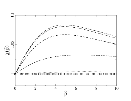
Figure 7: The dimensionless function $\chi(\tilde{\rho})$ defined in eq. (31), for various values of $\kappa/u=3\times 10^{n}$, with $n=2$ (circles), $n=1$ (squares), $n=0$ (diamonds), $n=-1,\cdots,-5$ from bottom to top.

Appendix B The functions $I_{3}^{(2)}(\kappa;\rho)$ and $J_{3}^{(3)}(p;\kappa;\rho)$

In this appendix we provide details about the functions $I_{3}^{(2)}(\kappa;\rho)$ and $J_{3}^{(3)}(p;\kappa;\rho)$ calculated with the propagators (17) and (22) respectively.

Consider first the function $I_{3}^{(2)}(\kappa;\rho)$, defined in eq. (11), and whose explicit expression is given in eq. (19). The variation of $I_{3}^{(2)}(\kappa;\rho)$ with $\kappa$ is dominated by the explicit linear $\kappa$ dependence and the $\kappa$-dependence of the renormalization factor $Z_{\kappa}$. The function

$$\frac{Z_{\kappa}I_{3}^{(2)}(\kappa;\rho)}{\kappa}=2K_{3}\frac{1}{(1+\hat{m}^{2}_{\kappa}(\tilde{\rho}))^{2}}\left(1-\frac{\eta_{\kappa}}{5}\right),$$ (38)

displayed in fig. 8, illustrates the remaining dependence on $\kappa$ and $\tilde{\rho}$.

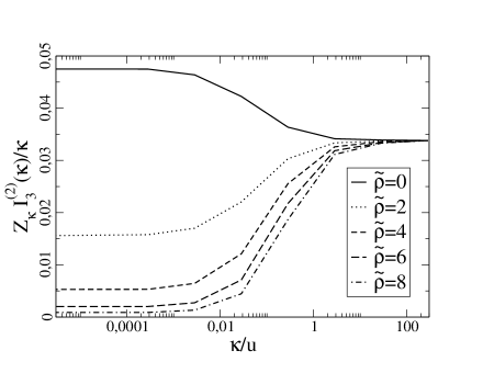
Figure 8: The function $Z_{\kappa}I_{3}^{2}(\kappa;\tilde{\rho})/\kappa$ as a function of $\kappa/u$, for different values of $\tilde{\rho}$.

Consider next $J_{3}^{(3)}(p;\kappa;\rho)$, defined in eq. (10). Using the LPA’ propagators of eqs. (17) and (22) one can calculate it analytically. One first makes the changes of variables $\bar{p}=p/\kappa,\bar{q}=q/\kappa$ and $\cos\gamma=p.q/p\;q$, and then perform the integral over the remaining angular variables. One gets then

$$J_{3}^{(3)}(p;\kappa;\rho) = \frac{1}{\kappa Z_{\kappa}^{2}(2\pi)^{2}}\frac{1}{(1+\hat{m}_{\kappa}^{2})^{2}}\int_{0}^{1}d\bar{q}\bar{q}^{2}\int_{-1}^{1}d(\cos\gamma)$$

$$\times\, \frac{(2-\eta+\eta\bar{q}^{2})}{\Theta(1\!-\!\bar{q}^{2}\!-\!\bar{p}^{2}\!+\!2\bar{q}\bar{p}\cos\gamma)\!+\!(\bar{q}^{2}\!+\!\bar{p}^{2}-2\bar{q}\bar{p}\cos\gamma)\Theta(\bar{q}^{2}\!+\!\bar{p}^{2}\!-\!2\bar{q}\bar{p}\cos\gamma\!-\!1)\!+\!\hat{m}_{\kappa}^{2}}.$$

To perform the integral over $\cos\gamma$ one needs to consider the various domains defined by the $\Theta$ functions. It is then convenient to separate the calculation in two different regions: $\bar{p}>2$ and $\bar{p}\leq 2$, and this for the two possible signs of $\hat{m}_{\kappa}^{2}$ (see also Blaizot:2005wd ). The calculation is then done by first integrating over $\cos\gamma$; the remaining integration over $\bar{q}$ can be done by making first an integration by parts to get a rational function, that is then decomposed into simple fractions. One finally gets (the dependence on $\tilde{\rho}$ is entirely contained in $\hat{m}_{\kappa}(\tilde{\rho})$ and is not written out explicitly):

a) $\bar{p}>2,\hat{m}_{\kappa}^{2}<0$.

$$J_{3}^{(3)}(p;\kappa;\tilde{\rho})=\frac{1}{\kappa Z_{\kappa}^{2}(2\pi)^{2}}\frac{1}{(1+\hat{m}_{\kappa}^{2})^{2}}\left\{2+\frac{\eta}{2}\left(-\frac{5}{3}+\bar{p}^{2}-3\hat{m}_{\kappa}^{2}\right)\right.$$

$$+\frac{1}{2\bar{p}}\left[-1+\frac{\eta}{4}+\left(\bar{p}+\sqrt{-\hat{m}_{\kappa}^{2}}\right)^{2}\left(1-\frac{\eta}{2}+\frac{\eta}{4}\left(\bar{p}+\sqrt{-\hat{m}_{\kappa}^{2}}\right)^{2}\right)\right]\log\left(\frac{\bar{p}-1+\sqrt{-\hat{m}_{\kappa}^{2}}}{\bar{p}+1+\sqrt{-\hat{m}_{\kappa}^{2}}}\right)$$

$$+\left.\frac{1}{2\bar{p}}\left[-1+\frac{\eta}{4}+\left(\bar{p}-\sqrt{-\hat{m}_{\kappa}^{2}}\right)^{2}\left(1-\frac{\eta}{2}+\frac{\eta}{4}\left(\bar{p}-\sqrt{-\hat{m}_{\kappa}^{2}}\right)^{2}\right)\right]\log\left(\frac{\bar{p}-1-\sqrt{-\hat{m}_{\kappa}^{2}}}{\bar{p}+1-\sqrt{-\hat{m}_{\kappa}^{2}}}\right)\right\}$$

$$=\frac{1}{\kappa Z_{\kappa}^{2}(2\pi)^{2}}\frac{2}{(1+\hat{m}_{\kappa}^{2})^{2}}\left\{\frac{4}{\bar{p}^{2}}\left(\frac{1}{3}-\frac{\eta}{15}\right)+\frac{4}{\bar{p}^{4}}\left(\frac{1}{15}-\frac{\eta}{105}-\frac{\hat{m}_{\kappa}^{2}}{3}+\frac{\eta\hat{m}_{\kappa}^{2}}{15}\right)+\mathcal{O}(1/(\bar{p}^{6}))\right\}.$$

b) $\bar{p}\leq 2,\hat{m}_{\kappa}^{2}<0$.

$$J_{3}^{(3)}(p;\kappa;\tilde{\rho}) = \frac{1}{\kappa Z_{\kappa}^{2}(2\pi)^{2}}\frac{1}{(1+\hat{m}_{\kappa}^{2})^{2}}\left\{-1+\frac{\eta}{4}+\frac{\eta\hat{m}_{\kappa}^{2}}{4}+\bar{p}\left(\frac{3}{2}-\frac{\eta}{8}-\frac{7\eta\hat{m}_{\kappa}^{2}}{8}\right)-\frac{3\eta}{4}\bar{p}^{2}\right.$$ (41)

$$+ \frac{25\eta}{48}\bar{p}^{3}+\frac{1}{1+\hat{m}_{\kappa}^{2}}\left(\frac{4}{3}-\frac{4\eta}{15}-\bar{p}+\frac{\eta}{3}\bar{p}^{2}+\left(\frac{1}{12}-\frac{\eta}{6}\right)\bar{p}^{3}+\frac{\eta}{120}\bar{p}^{5}\right)$$

$$+ \frac{1}{2\bar{p}}\left[1-\frac{\eta}{4}-\left(\bar{p}+\sqrt{-\hat{m}_{\kappa}^{2}}\right)^{2}\left(1-\frac{\eta}{2}+\frac{\eta}{4}\left(\bar{p}+\sqrt{-\hat{m}_{\kappa}^{2}}\right)^{2}\right)\right]\log\left(\frac{\bar{p}+1+\sqrt{-\hat{m}_{\kappa}^{2}}}{1+\sqrt{-\hat{m}_{\kappa}^{2}}}\right)$$

$$+ \left.\frac{1}{2\bar{p}}\left[1-\frac{\eta}{4}-\left(\bar{p}-\sqrt{-\hat{m}_{\kappa}^{2}}\right)^{2}\left(1-\frac{\eta}{2}+\frac{\eta}{4}\left(\bar{p}-\sqrt{-\hat{m}_{\kappa}^{2}}\right)^{2}\right)\right]\log\left(\frac{\bar{p}+1-\sqrt{-\hat{m}_{\kappa}^{2}}}{1-\sqrt{-\hat{m}_{\kappa}^{2}}}\right)\right\}$$

$$= \frac{1}{\kappa Z_{\kappa}^{2}(2\pi)^{2}}\frac{1}{(1+\hat{m}_{\kappa}^{2})^{2}}\left\{\frac{4}{3(1+\hat{m}_{\kappa}^{2})}\left(1-\frac{\eta}{5}\right)-\frac{2}{3(1+\hat{m}_{\kappa}^{2})^{2}}\bar{p}^{2}\right.$$

$$+ \left.\frac{2+\eta-2\hat{m}_{\kappa}^{2}+\eta\hat{m}_{\kappa}^{2}}{6(1+\hat{m}_{\kappa}^{2})^{3}}\bar{p}^{3}-\frac{2(1+\eta-5\hat{m}_{\kappa}^{2}+\eta\hat{m}_{\kappa}^{2})}{15(1+\hat{m}_{\kappa}^{2})^{4}}\bar{p}^{4}+\mathcal{O}(\bar{p}^{5})\right\}.$$

c) $\bar{p}>2,m_{\kappa}^{2}\geq 0$.

$$J_{3}^{(3)}(p;\kappa;\tilde{\rho})=\frac{1}{\kappa Z_{\kappa}^{2}(2\pi)^{2}}\frac{1}{(1+\hat{m}_{\kappa}^{2})^{2}}\left\{2+\frac{\eta}{2}\left(-\frac{5}{3}+\bar{p}^{2}-3\hat{m}_{\kappa}^{2}\right)\right.$$

$$+\frac{1}{\bar{p}}\left[\left(-1+\frac{\eta}{4}+(\bar{p}^{2}-\hat{m}_{\kappa}^{2})\left(1-\frac{\eta}{2}+\frac{\eta}{4}(\bar{p}^{2}-\hat{m}_{\kappa}^{2})\right)-\eta\hat{m}_{\kappa}^{2}\bar{p}^{2}\right)\frac{1}{2}\log\left(\frac{(\bar{p}-1)^{2}+\hat{m}_{\kappa}^{2}}{(\bar{p}+1)^{2}+\hat{m}_{\kappa}^{2}}\right)\right.$$

$$\left.\left.-2\hat{m}_{\kappa}\bar{p}\left(1-\frac{\eta}{2}+\frac{\eta}{2}(\bar{p}^{2}-\hat{m}_{\kappa}^{2})\right)\left(\mathrm{Arctan}\left(\frac{\hat{m}_{\kappa}}{\bar{p}-1}\right)-\mathrm{Arctan}\left(\frac{\hat{m}_{\kappa}}{\bar{p}+1}\right)\right)\right]\right\}$$

$$=\frac{1}{\kappa Z_{\kappa}^{2}(2\pi)^{2}}\frac{1}{(1+\hat{m}_{\kappa}^{2})^{2}}\left\{\frac{4}{\bar{p}^{2}}\left(\frac{1}{3}-\frac{\eta}{15}\right)\right.$$

$$\left.+\frac{1}{105\,\bar{p}^{4}}\left(7-35\hat{m}_{\kappa}^{2}+\eta(-1+7\hat{m}_{\kappa}^{2})\right)+\mathcal{O}(1/(\bar{p}^{6}))\right\}$$

d) $\bar{p}\leq 2,m_{\kappa}^{2}\geq 0$.

$$J_{3}^{(3)}(p;\kappa;\tilde{\rho}) = \frac{1}{\kappa Z_{\kappa}^{2}(2\pi)^{2}(1+\hat{m}_{\kappa}^{2})^{2}}\left\{-1+\frac{\eta}{4}+\frac{\eta\hat{m}_{\kappa}^{2}}{4}+\bar{p}\left(\frac{3}{2}-\frac{\eta}{8}-\frac{7\eta\hat{m}_{\kappa}^{2}}{8}\right)-\frac{3\eta\bar{p}^{2}}{4}\right.$$ (43)

$$+ \frac{25\eta\bar{p}^{3}}{48}+\frac{1}{1+\hat{m}_{\kappa}^{2}}\left(\frac{4}{3}-\frac{4\eta}{15}-\bar{p}+\frac{\eta\bar{p}^{2}}{3}+\frac{\bar{p}^{3}}{12}-\frac{\eta\bar{p}^{3}}{6}+\frac{\eta\bar{p}^{5}}{120}\right)$$

$$+ \frac{1}{\bar{p}}\left[\left(1-\frac{\eta}{4}-(\bar{p}^{2}-\hat{m}_{\kappa}^{2})\left(1-\frac{\eta}{2}+\frac{\eta}{4}(\bar{p}^{2}-\hat{m}_{\kappa}^{2})\right)+\eta\hat{m}_{\kappa}^{2}\bar{p}^{2}\right)\frac{1}{2}\log\left(\frac{(\bar{p}+1)^{2}+\hat{m}_{\kappa}^{2}}{1+\hat{m}_{\kappa}^{2}}\right)\right.$$

$$+ \left.\left.2\hat{m}_{\kappa}\bar{p}\left(1-\frac{\eta}{2}+\frac{\eta}{2}(\bar{p}^{2}-\hat{m}_{\kappa}^{2})\right)\left(\mathrm{Arctan}\left(\frac{\hat{m}_{\kappa}}{\bar{p}+1}\right)-\mathrm{Arctan}\left(\hat{m}_{\kappa}\right)\right)\right]\right\}$$

$$= \frac{1}{\kappa Z_{\kappa}^{2}(2\pi)^{2}(1+\hat{m}_{\kappa}^{2})^{2}}\left\{\frac{4}{3(1+\hat{m}_{\kappa}^{2})}\left(1-\frac{\eta}{5}\right)-\frac{2}{3(1+\hat{m}_{\kappa}^{2})^{2}}\bar{p}^{2}\right.$$

$$+ \left.\frac{2+\eta-2\hat{m}_{\kappa}^{2}+\eta\hat{m}_{\kappa}^{2}}{6(1+\hat{m}_{\kappa}^{2})^{3}}\bar{p}^{3}-\frac{2(1+\eta-5\hat{m}_{\kappa}^{2}+\eta\hat{m}_{\kappa}^{2})}{15(1+\hat{m}_{\kappa}^{2})^{4}}\bar{p}^{4}+\mathcal{O}(\bar{p}^{5})\right\}.$$

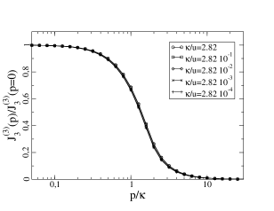
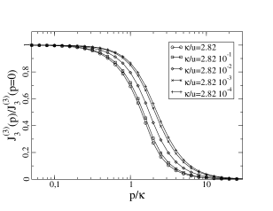
Figure 9: The function $J_{3}^{(3)}(\kappa;p)/I_{3}^{(3)}(\kappa)$ for $\tilde{\rho}=0$ (left) and $\tilde{\rho}=6$ (right), as a function of $(p/\kappa)$, for different values of $\kappa/u$.

The function $J_{3}^{(3)}(p;\kappa;\rho)/J_{3}^{(3)}(p=0;\kappa;\rho)$ is displayed in fig. 9 for the two values $\tilde{\rho}=0$, and $\tilde{\rho}=6$. One sees that in both cases the $p$-dependence is concentrated in the region $p\sim\kappa$: $J_{3}^{(3)}(p;\kappa;\rho)$ is independent of $p$ when $p\mathrel{\hbox to0.0pt{\raise 2.20013pt\hbox{$<$}\hss}{\lower 2.20013pt\hbox{$\sim$}}}\kappa$, and it vanishes when $p\mathrel{\hbox to0.0pt{\raise 2.20013pt\hbox{$>$}\hss}{\lower 2.20013pt\hbox{$\sim$}}}\kappa$, a property that has also been exploited in Blaizot:2005wd and Blaizot:2006vr . For $\tilde{\rho}=0$, $J_{3}^{(3)}(\kappa;p)/J_{3}^{(3)}(\kappa;p=0)$ is essentially a function of $p/\kappa$ only. For $\tilde{\rho}=6$ some residual dependence on $\kappa$ remains.

Appendix C Ultraviolet behavior of the self-energy

In this appendix we study the behavior of the self-energy $\Sigma(p)$ for $p\gg u$. We show that the solution of eq. (16) reproduces the result of 2-loop perturbation theory, namely $\Sigma(p)=u^{2}/(96\pi^{2})\log(p/u)$, albeit with a coefficient in front of the logarithmic that differs by 8%.

Consider first the exact flow equation for the 2-point function, eq. (5), in vanishing external field (in this appendix $\rho=0$ throughout). At order 0-loop (indicated by the superscript $[0]$), this is simply:

$$\partial_{\kappa}\Gamma_{\kappa}^{(2)[0]}(p)=0.$$ (44)

This equation has the solution

$$\Gamma_{\kappa}^{(2)[0]}(p)=p^{2},$$ (45)

where we used the initial condition at $\kappa=\Lambda$ that one deduces from eq. (1), and adjusted the bare mass $r$ to be at criticality ($\Sigma_{\kappa=0}(p=0;\rho=0)=0$, yielding $r^{[0]}=0$).

To go to 1-loop, one uses, in the r.h.s. of eq. (5), the 0-loop expressions for both the propagator, $G_{0}(\kappa;p)={1}/({p^{2}+R_{\kappa}(p)})$, and the 4-point function $\Gamma_{\kappa}^{(4)[0]}(p_{1},p_{2},p_{3}.p_{4})=u$. One gets

$$\partial_{\kappa}\Gamma_{\kappa}^{(2)[1]}(p) = -\frac{u}{2}\;\int\frac{d^{d}q}{(2\pi)^{d}}\frac{\partial_{\kappa}R_{\kappa}(q)}{(q^{2}+R_{\kappa}(q))^{2}}=\frac{u}{2}\partial_{\kappa}\int\frac{d^{d}q}{(2\pi)^{d}}\frac{1}{q^{2}+R_{\kappa}(q)}$$

The integration is immediate; by imposing criticality and the initial condition at $\kappa=\Lambda$, one obtains

$$\Gamma_{\kappa}^{(2)[1]}(p)=p^{2}+\frac{u}{2}\;\int\frac{d^{d}q}{(2\pi)^{d}}\left\{\frac{1}{q^{2}+R_{\kappa}(q)}-\frac{1}{q^{2}}\right\},$$ (47)

giving a self-energy which is in fact independent of the momentum $p$.

The 1-loop expression for the 4-point function, which will be needed shortly, is obtained similarly:

$$\!\!\!\!\!\!\!{\partial_{\kappa}\Gamma^{(4)[1]}_{\kappa}(p,-p,l,-l)}=$$

$$u^{2}\int\frac{d^{d}q}{(2\pi)^{d}}\partial_{\kappa}R_{\kappa}(q)G^{2}_{0}(\kappa;q)\left\{G_{0}(\kappa;q)+G_{0}(\kappa;p+l+q)+G_{0}(\kappa;p-l+q)\right\},$$ (48)

which can be integrated easily to give

$$\!\!\!\!\!\!\!\Gamma^{(4)[1]}_{\kappa}(p,-p,l,-l)=$$

$$u\!-\!\frac{u^{2}}{2}\int\frac{d^{d}q}{(2\pi)^{d}}G_{0}(\kappa;q)\left\{G_{0}(\kappa;q)+G_{0}(\kappa;p+l+q)+G_{0}(\kappa;p-l+q)\right\},$$

where we imposed the initial condition $\Gamma^{(4)}_{\kappa=\Lambda}(p,-p,l,-l,\rho=0)=u$ (the integrand in eq. (C) should, for finite $\Lambda$, be subtracted from its value at $\kappa=\Lambda$ in order to satisfy this initial condition; the corresponding contribution, however, vanishes in the limit $\Lambda\to\infty$, and we assume here that $\Lambda$ is large enough so that it can be neglected.)

Going now to 2-loop, one puts in the r.h.s. of eq. (5) the 1-loop expressions of both the propagator and the 4-point functions. Since we are interested only in the momentum dependence of the 2-point function, we consider only the terms in the flow equation that depend on $p$, i.e., $\Sigma_{\kappa}(p)=\Gamma^{(2)}_{\kappa}(p)-\Gamma^{(2)}_{\kappa}(0)-p^{2}$. Since the momentum dependent terms originate entirely from the contribution of order $u^{2}$ in $\Gamma^{(4)[1]}$, we can use $G_{0}$ as propagator. We have therefore

$$\partial_{\kappa}\Sigma_{\kappa}^{[2]}(p)=\frac{u^{2}}{2}\int\frac{d^{d}l}{(2\pi)^{d}}\partial_{\kappa}R_{\kappa}(l)G_{0}^{2}(\kappa;l)\int\frac{d^{d}q}{(2\pi)^{d}}G_{0}(\kappa;q)(G_{0}(\kappa;p+l+q)\!-\!G_{0}(\kappa;l+q)).$$

This expression can also be integrated to give

$$\Sigma_{\kappa}^{[2]}(p)=-\frac{u^{2}}{6}\int\frac{d^{d}l}{(2\pi)^{d}}\int\frac{d^{d}q}{(2\pi)^{d}}G_{0}(\kappa;l)G_{0}(\kappa;q)(G_{0}(\kappa;p+l+q)-G_{0}(\kappa;l+q)).$$ (51)

At this point, we need to deal with the fact that the 2-loop expression for the self-energy is IR divergent. And indeed when $\kappa\to 0$ at fixed $p$, the integral in eq. (51) diverges. In order to go around this difficulty, we consider the derivative $\partial_{p}\Delta\Gamma^{(2)}_{\kappa}(p)$

$$\frac{\partial\Sigma_{\kappa}^{[2]}(p)}{\partial|p|}=\frac{u^{2}}{3}\!\int\frac{d^{d}l}{(2\pi)^{d}}\int\frac{d^{d}q}{(2\pi)^{d}}G_{0}(l)G_{0}(q)G_{0}^{2}\;(p\!+\!l\!+\!q)({\bf l\!+\!q\!+\!p}).\hat{{\bf p}}\;(1+R_{\kappa}^{\prime}(l\!+\!p\!+\!q)),$$

where $\hat{{\bf p}}\equiv{\bf p}/|{\bf p}|$ and $R_{\kappa}^{\prime}(q)\equiv\partial_{q^{2}}R_{\kappa}(q)$. The limit $\kappa\to 0$ can now be taken, and yields

$$\frac{\partial\Sigma_{\kappa=0}^{[2]}(p)}{\partial|p|}=\frac{u^{2}}{6}\int\frac{d^{d}q}{(2\pi)^{d}}\frac{2q.\hat{p}}{q^{4}}\int\frac{d^{d}l}{(2\pi)^{d}}\frac{1}{l^{2}}\frac{1}{(l+p-q)^{2}}.$$ (53)

Performing the integral over $l$ and those over $\cos\theta=\hat{\bf p}.\hat{\bf q}$ and $|{\bf q}|$, one recovers the well known result ( in $d=3$):

$$\frac{\partial\Sigma_{\kappa=0}^{[2]}(p)}{\partial|p|} = \frac{1}{24}\frac{u^{2}}{(2\pi)2}\int_{0}^{\infty}\frac{d|q|}{|q|}\int_{0}^{\pi}d\theta\frac{\sin\theta\,\cos\theta}{(p^{2}+q^{2}-2|p||q|\cos\theta)^{1/2}}$$ (54)

$$= \frac{u^{2}}{96\pi^{2}}\frac{1}{|p|}.$$

Let us now turn to the perturbative limit of eq. (16). Note that, at both 0- and 1-loop orders, the predictions of eqs. (5) and (16) for the self-energy coincide. A difference arises at 2-loop order since, at the LO of the approximation scheme, we should insert in eq. (C) $\Gamma^{(4)[1]}_{\kappa}(p,-p,0,0)$ instead of $\Gamma^{(4)[1]}_{\kappa}(p,-p,l,-l)$ as we did in the exact calculation, where the expression of $\Gamma^{(4)[1]}$ is given in eq. (C). That is, the LO flow equation reads

$$\partial_{\kappa}\Sigma_{\kappa}^{[2]LO}(p)=\frac{u^{2}}{2}\int\frac{d^{d}l}{(2\pi)^{d}}\partial_{\kappa}R_{\kappa}(l)G_{0}^{2}(\kappa;l)\int\frac{d^{d}q}{(2\pi)^{d}}G_{0}(\kappa;q)(G_{0}(\kappa;p+q)-G_{0}(\kappa;q)).$$

In contrast to what happens with eq. (C), here the integration over $\kappa$ can no longer be done analytically and we have to deal with a third integral. Let us call $\kappa^{\prime}$ the variable of this integration, and integrate over $t^{\prime}=\log(\kappa^{\prime}/|p|)$. After making the changes of variables $q\to|p|q$ and $l\to|p|l$, one obtains:

$$\Sigma_{\kappa}^{(2)[2]LO}(p)=-\frac{u^{2}}{2}|p|^{2(d-3)}$$

$$\times\int_{\log\kappa/|p|}^{\infty}dt\int\frac{d^{d}l}{(2\pi)^{d}}\partial_{t^{\prime}}R_{\kappa^{\prime}}(l)G_{0}^{2}(\kappa;l)\int\frac{d^{d}q}{(2\pi)^{d}}G_{0}(\kappa;q)(G_{0}(\kappa;\hat{p}+q)-G_{0}(\kappa;q)).$$

Now, the derivative with respect to $|p|$ is very simple because, in $d=3$, it only enters in the integration limit. One has:

$$\frac{\partial{\Sigma_{\kappa}^{(2)[2]LO}(p)}}{\partial|p|}=-\frac{u^{2}}{2|p|}\int\frac{d^{3}l}{(2\pi)^{3}}\partial_{t}R_{\kappa}(l)G_{0}^{2}(\kappa;l)\int\frac{d^{3}q}{(2\pi)^{3}}G_{0}(\kappa;q)(G_{0}(\kappa;\hat{p}+q)-G_{0}(q)),$$

where $t=\log(\kappa/|p|)$. In can be verified that the first term, i.e., that containing $\hat{p}$, vanishes when $\kappa\ll|p|$. In this limit:

$$\frac{\partial{\Sigma_{\kappa=0}^{[2]LO}(p)}}{\partial|p|} = \frac{1}{2}\frac{u^{2}}{|p|}\int\frac{d^{3}l}{(2\pi)^{3}}\partial_{t}R_{\kappa}(l)G_{0}^{2}(\kappa;l)\int\frac{d^{3}q}{(2\pi)^{3}}G^{2}_{0}(\kappa;q)$$ (58)

$$= \frac{u^{2}}{9\pi^{4}}\frac{1}{|p|}.$$

Comparing eqs. (54) and (58) one sees that they both predict a logarithmic behavior for the self-energy, the ratio of their respective coefficients being:

$$\frac{1/(9\pi^{4})}{1/(96\pi^{2})}\simeq 1.08.$$ (59)

References

[1] C.Wetterich, Phys. Lett., B301, 90 (1993).
[2] U.Ellwanger, Z.Phys., C58, 619 (1993).
[3]
N. Tetradis and C. Wetterich,
Nucl. Phys. B 422, 541 (1994).
[4] T.R.Morris, Int. J. Mod. Phys., A9, 2411 (1994).
[5]
T. R. Morris,
Phys. Lett. B329 (1994) 241–248.
[6]
C. Bagnuls and C. Bervillier,
Phys. Rept. 348, 91 (2001).
[7]
J. Berges, N. Tetradis and C. Wetterich,
Phys. Rept. 363, 223–386 (2002).
[8] U. Ellwanger, Z. Phys., C62 (1994), 503;
U. Ellwanger and C. Wetterich, Nucl. Phys. B423 (1994), 137;
T. R. Morris, Phys. Lett. B 334 (1994) 355; U. Ellwanger,
M. Hirsch and A. Weber,
Eur. Phys. J. C 1 (1998) 563;
J. M. Pawlowski, D. F. Litim, S. Nedelko and L. von Smekal,
Phys. Rev. Lett. 93 (2004) 152002;
J. Kato,
arXiv:hep-th/0401068; C. S. Fischer and H. Gies,
JHEP 0410 (2004) 048; N. Hasselmann, S. Ledowski and
P. Kopietz, Phys. Rev. A69, 061601(R) (2004) and
Phys. Rev. A70, 063621 (2004).
[9]
S. Weinberg, Phys. Rev. D8 (1973) 3497.
[10] G. R. Golner, Exact renormalization group flow equations for free
energies and N-point functions in uniform external fields,
arXiv:hep-th/9801124.
[11] Parola, A., and Reatto, L., Adv. Phys. 44 (1995) 211;
Parola, A., Reatto, L., and Pini, D., Phys. Rev. E. 48 (1993), 3321.
[12]
L. Canet, B. Delamotte, D. Mouhanna and J. Vidal,
Phys. Rev. B68 (2003) 064421.
[13] B. Delamotte, D. Mouhanna, M. Tissier, Phys. Rev. B69, 134413 (2004); L. Canet and B. Delamotte, cond-matt/0412205.
[14]
J. P. Blaizot, R. Mendez Galain and N. Wschebor,
Phys. Lett. B 632, 571 (2006)
[15]
J. P. Blaizot, R. Mendez-Galain and N. Wschebor,
arXiv:hep-th/0512317.
[16]
J. P. Blaizot, R. Mendez-Galain and N. Wschebor,
arXiv:hep-th/0603163.
[17]
R.D. Ball, P.E. Haagensen, J.I. Latorre, and E. Moreno, Phys. Lett.
B347 (1995) 80.