Relativistic Wave Equations and Compton Scattering

Abstract

The recently proposed eight-component relativistic wave equation is applied to the scattering of a photon from a free electron (Compton scattering). It is found that in spite of the considerable difference in the structure of this equation and that of Dirac the cross section is given by the Klein-Nishina formula.

1 Introduction

Recently an eight-component relativistic wave equation for spin-$\frac{1}{2}$ particles was proposed [1, 2]. This equation was obtained from a four-component spin-$\frac{1}{2}$ wave equation (the KG$\frac{1}{2}$ equation [2]), which contains second-order derivatives in both space and time, by a procedure involving a linearization of the time derivative analogous to that introduced by Feshbach and Villars [3] for the Klein-Gordon equation. This new eight-component equation gives the same bound-state energy eigenvalue spectra for hydrogenic atoms as the Dirac equation but has been shown to predict different radiative transition probabilities for the fine structure of both the Balmer and Lyman $\alpha$-lines [4]. Since it has been shown that the new theory does not always give the same results as the Dirac theory, it is important to consider the validity of the new equation in the case of other physical problems. One of the early crucial tests of the Dirac theory was its application to the scattering of a photon by a free electron : the so-called Compton scattering problem. In this paper we apply the new theory to the calculation of Compton scattering to order $e^{2}$. For this problem it is easier to calculate the result using the four-component KG$\frac{1}{2}$ equation and this is carried out in Section 2. However, for completeness, the calculation for the eight-component theory is given in Section 3 and is shown to be equivalent to that obtained by the four-component theory, namely the well-known Klein-Nishina formula [5, 6] initially obtained using the Dirac theory.

2 Four-component (KG$\frac{1}{2}$ equation) theory for Compton scattering

The four-component KG$\frac{1}{2}$ equation [2] is

$$\left[\left(D_{\mu}D^{\mu}+m^{2}\right)\mbox{\boldmath$1_{4}$}+\frac{e}{2}\sigma^{\mu\nu}F_{\mu\nu}\right]\Psi=0$$ (II.1)

where $\sigma^{\mu\nu}=\frac{i}{2}\left[\gamma^{\mu},\gamma^{\nu}\right]$, $F_{\mu\nu}=\partial_{\mu}A_{\nu}-\partial_{\nu}A_{\mu}$ and $\gamma^{\mu}$ are the standard Dirac matrices :

$$\begin{array}[]{lr}\gamma^{0}=\left[\begin{array}[]{cc}\mbox{\boldmath$1_{2}$}&\mbox{\boldmath$0$}\\ \mbox{\boldmath$0$}&\mbox{\boldmath$-1_{2}$}\end{array}\right]&\mbox{\boldmath$\gamma$}=\left[\begin{array}[]{cc}\mbox{\boldmath$0$}&\mbox{\boldmath$\sigma$}\\ \mbox{\boldmath$-\sigma$}&\mbox{\boldmath$0$}\end{array}\right]\end{array}.$$ (II.2)

The final term is the spin interaction term in the presence of an external electromagnetic field. Eq. (II.1) reduces to the free particle Klein-Gordon type equation in the absence of a field

$$\left\{\partial_{\mu}\partial^{\mu}+m^{2}\right\}\mbox{\boldmath$1_{4}$}\Psi=0.$$ (II.3)

The free particle positive energy solution of (II.3), normalized within a box of volume $L^{3}$ may be written

$$\Psi=\frac{e^{-ip\cdot x}}{\sqrt{2EL^{3}}}u(p,s)$$ (II.4)

where

$$u(p,s)=\frac{1}{\sqrt{2mE_{+}}}\left[\begin{array}[]{c}E_{+}\phi_{s}\\ \left(\mbox{\boldmath$\sigma\cdot p$}\right)\phi_{s}\end{array}\right].$$ (II.5)

Here $p$ is the four-momentum of the electron of energy $E$, $E_{+}$ = $E$ + $m$ and $\phi_{s}$ is a normalized two component spinor in the rest frame. Compton scattering refers to the scattering of photons by free electrons. The lowest order Feynman diagrams for this process are shown in Figure 1. There are three diagrams : (a) direct, (b) exchange and (c) “seagull”.

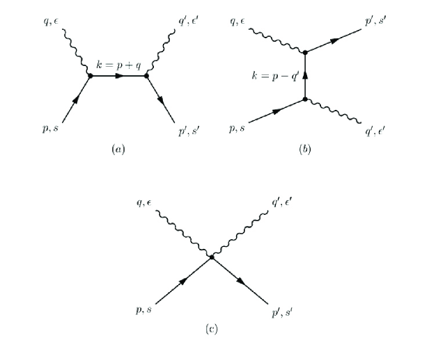
Figure 1: Feynman diagrams for Compton scattering.

The perturbing interaction causing the scattering is given by

$$V(x)=ie\left(\partial_{\mu}A^{\mu}+A_{\mu}\partial^{\mu}\right)+\frac{e}{2}\sigma^{\mu\nu}F_{\mu\nu}-e^{2}A^{\mu}A_{\mu}$$ (II.6)

where $A_{\mu}$ is the four-vector electromagnetic potential satisfying

$$\partial_{\mu}\partial^{\mu}A_{\nu}=0.$$ (II.7)

The direct and exchange diagrams correspond to the first and second terms in the potential $V(x)$. The “seagull” diagram arises from the third term in Eq. (II.6).

To describe an incoming (outgoing) photon of polarization vector $\epsilon_{\mu}$ ($\epsilon_{\mu}^{\prime}$) we choose the plane wave solutions of (II.7) to be of the form

$$A^{\mu}(x,q)=\frac{1}{\sqrt{2q^{0}L^{3}}}\epsilon^{\mu}(q,\lambda)e^{-iq\cdot x}$$ (II.8)

and

$$A^{\mu}(x,q^{\prime})=\frac{1}{\sqrt{2q^{\prime 0}L^{3}}}\epsilon^{\prime\mu}(q^{\prime},\lambda^{\prime})e^{+iq^{\prime}\cdot x}$$ (II.9)

respectively, where $q$, $q^{\prime}$ are the four-momenta of the photons, $q^{2}$ = $q^{\prime 2}$ = 0 and $\lambda,\lambda^{\prime}$ define the photon polarization states.

The differential cross section for Compton scattering is given by

$$d\sigma=\int\frac{\left|a_{fi}\right|^{2}}{\left|\mbox{\boldmath$j$}\right|T}dN$$ (II.10)

where $\left|a_{fi}\right|^{2}$ is the transition probability, $T$ is the time interval, $j$ is the incident particle flux, and $N$ is the number of final states. The transition matrix from standard pertubation theory may be written

$$a_{fi} = i\int d^{4}x\bar{\Psi}_{f}(x)V(x)\Psi_{i}(x)$$ (II.11)

$$+ i\int\int d^{4}xd^{4}y\bar{\Psi}_{f}(x)V(x)G(x-y)V(y)\Psi_{i}(y)$$

$$+ ...$$

where $\bar{\Psi}$ = $\Psi^{\dagger}\gamma_{0}$ and the Green function

$$G(x-y)=\int{\frac{d^{4}k}{(2\pi)^{4}}e^{-ik\cdot(x-y)}G(k)}$$ (II.12)

with

$$G(k)=\frac{1}{k^{2}-m^{2}}\mbox{\boldmath$1_{4}$}.$$ (II.13)

To the lowest order in e, the transition matrix for Compton scattering is, from Eqs. (II.6) and (II.11)

$$a_{fi} = -ie^{2}\int d^{4}x\bar{\Psi}_{f}(x)[A^{\mu}(x,q^{\prime})A_{\mu}(x,q)+A^{\mu}(x,q)A_{\mu}(x,q^{\prime})]\Psi_{i}(x)$$ (II.14)

$$- ie^{2}\int\int d^{4}xd^{4}y\bar{\Psi}_{f}\left[\left(\partial^{\mu}A_{\mu}+A_{\mu}\partial^{\mu}-\frac{i}{2}\sigma^{\mu\nu}F_{\mu\nu}\right)_{(x,q)}G(x-y)\right.$$

$$\times \left.\left(\partial^{\mu}A_{\mu}+A_{\mu}\partial^{\mu}-\frac{i}{2}\sigma^{\mu\nu}F_{\mu\nu}\right)_{(y,q^{\prime})}\right.$$

$$+ \left.\left(\partial^{\mu}A_{\mu}+A_{\mu}\partial^{\mu}-\frac{i}{2}\sigma^{\mu\nu}F_{\mu\nu}\right)_{(x,q^{\prime})}G(x-y)\right.$$

$$\times \left.\left(\partial^{\mu}A_{\mu}+A_{\mu}\partial^{\mu}-\frac{i}{2}\sigma^{\mu\nu}F_{\mu\nu}\right)_{(y,q)}\right]\Psi_{i}(y)$$

where the bracketed subscripts $(x,q)$ denote the arguments of $\partial_{\mu}$ and $A_{\mu}$.

To evaluate Eq. (II.14) it is convenient to choose the laboratory frame with the target electron at rest, for which

$$p_{\mu}=(m,{\bf 0})\hskip 19.91692ptq_{\mu}=(\omega,{\bf q})\hskip 14.22636pt\mbox{with}\hskip 14.22636pt\omega=\left|{\bf q}\right|$$

$$p^{\prime}_{\mu}=(E^{\prime},{\bf p}^{\prime})\hskip 19.91692ptq_{\mu}^{\prime}=(\omega^{\prime},{\bf q}^{\prime})\hskip 8.53581pt\mbox{with}\hskip 11.38109pt\omega^{\prime}=\left|\bf{q}^{\prime}\right|$$ (II.15)

and the special gauge in which the initial and final photons are transversely polarized in laboratory frame :

$$\epsilon_{\mu}=(0,\mbox{\boldmath$\epsilon$})\hskip 14.22636pt\mbox{with}\hskip 14.22636pt\mbox{\boldmath$\epsilon\cdot q$}=0$$

$$\epsilon_{\mu}^{\prime}=(0,\mbox{\boldmath$\epsilon^{\prime}$})\hskip 11.38109pt\mbox{with}\hskip 14.22636pt\mbox{\boldmath$\epsilon^{\prime}\cdot q^{\prime}$}=0.$$ (II.16)

Inserting Eqs. (II.4), (II.8), (II.9), and (II.12) into Eq. (II.14) and carrying out the integration over $d^{4}y$, $d^{4}k$ and $d^{4}x$ gives

$$a_{fi}=\frac{ie^{2}(2\pi)^{4}}{\sqrt{2E2E^{\prime}2\omega 2\omega^{\prime}L^{12}}}\delta^{4}(p^{\prime}+q^{\prime}-p-q)\left[\bar{u}(p^{\prime},s^{\prime})\Gamma u(p,s)\right]$$ (II.17)

where

$$\Gamma=\frac{(2p^{\prime}\cdot\epsilon^{\prime}-\not\!q^{\prime}\not\!\epsilon^{\prime})\not\!q\not\!\epsilon}{2p\cdot q}+\frac{(2p^{\prime}\cdot\epsilon+\not\!q\not\!\epsilon)\not\!q^{\prime}\not\!\epsilon^{\prime}}{2p\cdot q^{\prime}}-2(\epsilon\cdot\epsilon^{\prime})\mbox{\boldmath$1_{4}$}.$$ (II.18)

It should be noted that the factor of two in the last term involving $\epsilon^{\prime}\cdot\epsilon$ arises from two equal contributions to the seagull diagram (i.e. $\epsilon^{\prime}\cdot\epsilon$ + $\epsilon\cdot\epsilon^{\prime}$). In (II.18) the slash notation $\not\!\!A$ = $\gamma^{0}A^{0}$ - $\gamma\cdot A$ has been used.

Using Eqs. (II.10) and (II.16) and the Compton relation

$$\frac{\omega}{\omega^{\prime}}=1+\frac{\omega}{m}(1-\cos\theta)$$ (II.19)

where the final photon is scattered by an angle $\theta$ into the spherical angle element $d\Omega_{q^{\prime}}$ with respect to the incident photon, the differential cross section is

$$\frac{d\sigma}{d\Omega_{q^{\prime}}}(\lambda^{\prime},\lambda;s^{\prime},s)=\alpha^{2}\frac{\omega^{\prime 2}}{\omega^{2}}\frac{1}{4m^{2}}\left|\bar{u}(p^{\prime},s^{\prime})\Gamma u(p,s)\right|^{2}.$$ (II.20)

Here $\alpha$ is the fine structure constant $e^{2}/4\pi$ and $\lambda,\lambda^{\prime}$ are the initial and final photon polarizations.

Averaging over the initial electron spins and summing over the final electron spins gives

$$\frac{d\bar{\sigma}}{d\Omega_{q^{\prime}}}(\lambda^{\prime},\lambda)=\frac{1}{2}\sum_{s^{\prime},s}\frac{d\sigma}{d\Omega_{q^{\prime}}}(\lambda^{\prime},\lambda;s^{\prime},s).$$ (II.21)

The electron spinors can be eliminated employing the usual trace techniques [7] and Eq. (II.21) gives

$$\frac{d\bar{\sigma}}{d\Omega_{q^{\prime}}}(\lambda^{\prime},\lambda)=\alpha^{2}\frac{\omega^{\prime 2}}{\omega^{2}}\frac{1}{8m^{2}}Tr\left[\frac{\not\!p^{\prime}+m}{2m}\Gamma\frac{\not\!p+m}{2m}\bar{\Gamma}\right]$$ (II.22)

where

$$\bar{\Gamma}=\gamma_{0}\Gamma^{\dagger}\gamma_{0}.$$ (II.23)

The calculation of the trace in Eq. (II.22) is rather tedious, involving products of up to ten $\gamma$ matrices. However, the result is quite simple :

$$Tr\left[\frac{\not\!p^{\prime}+m}{2m}\Gamma\frac{\not\!p+m}{2m}\bar{\Gamma}\right]=8(\epsilon\cdot\epsilon^{\prime})^{2}+\frac{2(q\cdot q^{\prime})^{2}}{(p\cdot q)(p\cdot q^{\prime})}.$$ (II.24)

Now $(q\cdot q^{\prime})=\omega\omega^{\prime}(1-\cos\theta)$, $(p\cdot q)=m\omega$ and $(p\cdot q^{\prime})=m\omega^{\prime}$ so that

$$\frac{d\bar{\sigma}}{d\Omega_{q^{\prime}}}(\lambda,\lambda^{\prime})=\frac{\alpha^{2}}{2m^{2}}\left(\frac{\omega^{\prime}}{\omega}\right)\left[4(\epsilon\cdot\epsilon^{\prime})^{2}+\frac{\omega\omega^{\prime}}{m^{2}}(1-\cos\theta)^{2}\right]$$ (II.25)

which is identical to the Klein-Nishina formula derived using the Dirac equation [5, 6].

3 Eight-component theory for Compton scattering

The eight-component relativistic wave equation is obtained [1] from the KG$\frac{1}{2}$ equation by linearizing the time derivative using a procedure analogous to that employed by Feshbach and Villars [3] for the Klein-Gordon equation. The eight-component (FV$\frac{1}{2}$ equation) has the following form

$$i\frac{\partial}{\partial t}\mbox{\boldmath$1_{8}$}\Psi_{FV\frac{1}{2}}=H_{FV\frac{1}{2}}\Psi_{FV\frac{1}{2}}$$ (III.26)

where

$$H_{FV\frac{1}{2}}=(\tau_{3}+i\tau_{2})\otimes\frac{1}{2m}\left[-\mbox{\boldmath$D$}^{2}\mbox{\boldmath$1_{4}$}+\frac{e}{2}\sigma^{\mu\nu}F_{\mu\nu}\right]+m(\tau_{3}\otimes\mbox{\boldmath$1_{4}$})+eA_{0}\mbox{\boldmath$1_{8}$}.$$ (III.27)

In Eq. (III.27) $\tau_{i}$ are the standard Pauli matrices and $\otimes$ is the usual Kronecker (direct) product.

The free positive energy electron solution of (III.26), normalized within a box of volume $L^{3}$, may be written

$$\Psi_{FV\frac{1}{2}}=\frac{1}{2m}\left(\begin{array}[]{c}E_{+}\\ -E_{-}\end{array}\right)e^{-ip\cdot x}\otimes u(p,s)$$ (III.28)

where $E_{\pm}=E\pm m$ and the inner product can be written [2] as

$$\left<\Psi_{FV\frac{1}{2}}|\Psi_{FV\frac{1}{2}}\right>=\int\Psi_{FV\frac{1}{2}}^{\dagger}(x)\tau_{4}\Psi_{FV\frac{1}{2}}(x)d^{3}x$$ (III.29)

where $\tau_{4}=\tau_{3}\otimes\gamma_{0}$.

The differential cross section for Compton scattering is given by Eq. (II.10). In the eight-component theory, the transition matrix is

$$a_{fi} = i\int d^{4}x\Psi_{f}^{\dagger}(x)\tau_{4}V(x)\Psi_{i}(x)$$ (III.30)

$$+ i\int\int d^{4}xd^{4}y\Psi_{f}^{\dagger}(x)\tau_{4}V(x)G(x-y)V(y)\Psi_{i}(x)$$

$$+ ...$$

where now the Green function $G(x-y)$ is given by Eq. (II.12) but with

$$G(k)=\frac{1}{k^{2}-m^{2}}\left[\begin{array}[]{cc}\frac{\mbox{\boldmath$k$}^{2}}{2m}+m+k_{0}&\frac{\mbox{\boldmath$k$}^{2}}{2m}\\ -\frac{\mbox{\boldmath$k$}^{2}}{2m}&-\frac{\mbox{\boldmath$k$}^{2}}{2m}-m+k_{0}\end{array}\right]\otimes\mbox{\boldmath$1_{4}$}$$ (III.31)

The perturbing interaction is

$$V(x) = \frac{1}{2m}(\tau_{3}+i\tau_{2})$$ (III.32)

$$\otimes \left[ie\left(\{\mbox{\boldmath$\nabla\cdot A$}+\mbox{\boldmath$A\cdot\nabla$}\}\bf{1_{4}}\right)+\frac{e}{2}\sigma^{\mu\nu}F_{\mu\nu}+e^{2}(\mbox{\boldmath$A\cdot A$})\bf{1_{4}}\right].$$

Inserting (III.32) into Eq. (III.30) gives to second order in $e$

$$a_{fi} = \frac{ie^{2}}{2m}\int d^{4}x\Psi_{f}^{\dagger}(x)\tau_{4}(\tau_{3}+i\tau_{2})\otimes\mbox{\boldmath$A$}(x,q)\cdot\mbox{\boldmath$A$}(x,q^{\prime})\Psi_{i}(x)$$ (III.33)

$$- \frac{ie^{2}}{4m^{2}}\int\int d^{4}xd^{4}y\Psi_{f}^{\dagger}(x)$$

$$\times \tau_{4}\left[(\tau_{3}+i\tau_{2})\otimes\left((\not\!\partial\not\!\!A)+\left\{\mbox{\boldmath$\nabla\cdot A$}+\mbox{\boldmath$\nabla\cdot A$}\right\}\bf{1_{4}}\right)\right]_{(x,q)}G(x-y)$$

$$\times \tau_{4}\left[(\tau_{3}+i\tau_{2})\otimes\left((\not\!\partial\not\!\!A)+\left\{\mbox{\boldmath$\nabla\cdot A$}+\mbox{\boldmath$\nabla\cdot A$}\right\}\bf{1_{4}}\right)\right]_{(y,q^{\prime})}$$

$$+ \tau_{4}\left[(\tau_{3}+i\tau_{2})\otimes\left((\not\!\partial\not\!\!A)+\left\{\mbox{\boldmath$\nabla\cdot A$}+\mbox{\boldmath$\nabla\cdot A$}\right\}\bf{1_{4}}\right)\right]_{(x,q^{\prime})}G(x-y)$$

$$\times \tau_{4}\left[(\tau_{3}+i\tau_{2})\otimes\left((\not\!\partial\not\!\!A)+\left\{\mbox{\boldmath$\nabla\cdot A$}+\mbox{\boldmath$\nabla\cdot A$}\right\}\bf{1_{4}}\right)\right]_{(y,q)}\Psi_{i}(y)$$

where the use of brackets in $\not\!\partial\not\!\!A$ will mean that $\not\!\partial$ operates only within the brackets.

As already seen in Section 2, to second order in $e$, the amplitude for Compton scattering involves the three Feynman diagrams shown in Figure 1. Evaluation of Eq. (III.33) choosing the laboratory frame with the target electron at rest and the special transverse gauge in which the initial and final photons are transversely polarized in laboratory frames gives

$$a_{fi} = \frac{ie^{2}(2\pi)^{4}}{8m^{3}\sqrt{2\omega 2\omega^{\prime}L^{12}}}\delta^{4}(p^{\prime}+q^{\prime}-p-q)(E_{+},-E_{-})$$ (III.36)

$$\otimes u^{\dagger}(p^{\prime},s^{\prime})\tau_{4}[\frac{1}{2p\cdot q}((\tau_{3}+i\tau_{2})\otimes(-2\mbox{\boldmath$p^{\prime}\cdot\epsilon^{\prime}$}-\not\!q^{\prime}\not\!\epsilon^{\prime})\not\!q\not\!\epsilon)$$

$$+ \frac{1}{2p\cdot q^{\prime}}((\tau_{3}+i\tau_{2})\otimes(-2\mbox{\boldmath$p^{\prime}\cdot\epsilon$}+\not\!q\not\!\epsilon)\not\!q^{\prime}\not\!\epsilon^{\prime})$$

$$+ 2(\mbox{\boldmath$\epsilon\cdot\epsilon^{\prime}$})(\tau_{3}+i\tau_{2})\otimes\mbox{\boldmath$1_{4}$}]\left(\begin{array}[]{c}E_{+}\\ -E_{-}\end{array}\right)\otimes u(p,s).$$

Using 4 x 4 block matrices, it is readily shown that the expression (III.36) reduces to

$$a_{fi}=\frac{ie^{2}(2\pi)^{4}}{2m\sqrt{2\omega 2\omega^{\prime}L^{12}}}\delta^{4}(p^{\prime}+q^{\prime}-p-q)\left\{u^{\dagger}(p^{\prime},s^{\prime})\gamma^{0}\Gamma u(p,s)\right\}$$ (III.37)

where

$$\Gamma = \left[\frac{1}{2p\cdot q}((-2\mbox{\boldmath$p^{\prime}\cdot\epsilon^{\prime}$}-\not\!q^{\prime}\not\!\epsilon^{\prime})\not\!q\not\!\epsilon)\right.$$ (III.38)

$$+ \left.\frac{1}{2p\cdot q^{\prime}}((-2\mbox{\boldmath$p^{\prime}\cdot\epsilon$}+\not\!q\not\!\epsilon)\not\!q^{\prime}\not\!\epsilon^{\prime})+2(\mbox{\boldmath$\epsilon\cdot\epsilon^{\prime}$})\bf{1_{4}}\right].$$

For the special transverse gauge (II.16), Eq. (III.38) is identical with Eq. (II.18) so that the differential cross section for Compton scattering is once again the Klein-Nishina formula of Eq. (II.25).

4 Conclusion

It has been shown that to order $e^{2}$ both the second order KG$\frac{1}{2}$ equation and its eight-component form give the Klein-Nishina formula for the Compton scattering problem. This is the same result as obtained by the standard Dirac theory, although the new theory involves an additional “seagull” Feynman diagram.

References

References

[1] Robson B A and Staudte D S 1996 J. Phys. A : Math. Gen.29 157
[2] Staudte D S 1996 J. Phys. A : Math. Gen.29 169
[3] Feshbach H and Villars F 1958 Rev. Mod. Phys.30 24
[4] Robson B A and Sutanto S, submitted for publication
[5] Klein O and Nishina Y 1929 Z. Phys.52 853
[6] Greiner W and Reinhardt J 1992 Quantum Electrodynamics 2nd Edition [Berlin : Springer] p. 183
[7] Aitchison I J 1972 Relativistic Quantum Mechanics [London : MacMillan] p. 149