hep-th/0605234

Nordita-2006-14

Quantum Mechanical Sectors in

Thermal $\mathcal{N}=4$ Super Yang-Mills on $\mathbb{R}\times S^{3}$

Troels Harmark and Marta Orselli

The Niels Bohr Institute and Nordita
Blegdamsvej 17, 2100 Copenhagen Ø, Denmark

harmark@nbi.dk, orselli@nbi.dk

Abstract

We study the thermodynamics of $U(N)$ $\mathcal{N}=4$ Super Yang-Mills (SYM) on $\mathbb{R}\times S^{3}$ with non-zero chemical potentials for the $SU(4)$ R-symmetry. We find that when we are near a point with zero temperature and critical chemical potential, $\mathcal{N}=4$ SYM on $\mathbb{R}\times S^{3}$ reduces to a quantum mechanical theory. We identify three such critical regions giving rise to three different quantum mechanical theories. Two of them have a Hilbert space given by the $SU(2)$ and $SU(2|3)$ sectors of $\mathcal{N}=4$ SYM of recent interest in the study of integrability, while the third one is the half-BPS sector dual to bubbling AdS geometries. In the planar limit the three quantum mechanical theories can be seen as spin chains. In particular, we identify a near-critical region in which $\mathcal{N}=4$ SYM on $\mathbb{R}\times S^{3}$ essentially reduces to the ferromagnetic $XXX_{1/2}$ Heisenberg spin chain. We find furthermore a limit in which this relation becomes exact.

1 Introduction

The thermodynamics of large $N$ $U(N)$ $\mathcal{N}=4$ Super Yang-Mills (SYM) on $\mathbb{R}\times S^{3}$ has proven to be interesting for several reasons. It has a confinement/deconfinement phase transition like in QCD that can be studied even at weak coupling [1]. This phase transition is conjectured to correspond to the Hagedorn phase transition for the dual type IIB string theory on ${\rm AdS}_{5}\times S^{5}$, which is in accordance with the fact that the large $N$ $\mathcal{N}=4$ SYM theory has a Hagedorn spectrum [2, 3, 4]. This is very interesting since it means that we can study what happens beyond the Hagedorn transition on the weakly coupled gauge theory side. For large coupling the same phase transition corresponds to the Hawking-Page phase transition for black holes in Anti-De Sitter space, which is a phase transition in semi-classical gravity [5, 1]. Thus, by studying the thermodynamics of $\mathcal{N}=4$ SYM we can hope to learn about such important subjects as what is beyond the Hagedorn transition, confinement in QCD and phase transitions in gravity.

In this paper we find that thermal $U(N)$ $\mathcal{N}=4$ SYM has quantum mechanical sectors, by which we mean that near certain critical points most of the degrees of freedom of $\mathcal{N}=4$ SYM can be integrated out and only a small subset, that we can regard as quantum mechanical, remains. These critical points arise in the study of the thermodynamics of $U(N)$ $\mathcal{N}=4$ SYM on $\mathbb{R}\times S^{3}$ with non-zero chemical potentials corresponding to the three R-charges for the $SU(4)$ R-symmetry of $\mathcal{N}=4$ SYM. Our main result is that when we are near a point with zero temperature and critical chemical potentials, $\mathcal{N}=4$ SYM reduces to one out of three simple quantum mechanical theories. Furthermore, for large $N$ these three quantum mechanical theories are mapped in a precise way to spin chain theories.

Denoting the three chemical potentials of $\mathcal{N}=4$ SYM as $\Omega_{1}$, $\Omega_{2}$, $\Omega_{3}$ and setting $\Omega_{1}=\Omega_{2}=\Omega$, $\Omega_{3}=0$, we can write one of the near-critical regions that we study as

$$T\ll 1\ ,\ \ 1-\Omega\ll 1\ ,\ \ \lambda\ll 1$$ (1.1)

where $T$ is the temperature and $\lambda$ is the ’t Hooft coupling of $\mathcal{N}=4$ SYM. In this region we are close to the critical point $(T,\Omega_{1},\Omega_{2},\Omega_{3})=(0,1,1,0)$. We show in this paper that in the region (1.1) $\mathcal{N}=4$ SYM on $\mathbb{R}\times S^{3}$ reduces to a quantum mechanical theory with the Hilbert space consisting of all multi-trace operators made out of the letters $Z$ and $X$, where $Z$ and $X$ are complex scalars of $\mathcal{N}=4$ SYM with R-symmetry weights $(1,0,0)$ and $(0,1,0)$. This is precisely the so-called $SU(2)$ sector that has been discussed in recent developments on the integrability of $\mathcal{N}=4$ SYM [6, 7, 8, 9, 10].

We find that it is natural to reformulate $\mathcal{N}=4$ SYM in the region (1.1) in terms of the rescaled temperature $\tilde{T}\equiv T/(1-\Omega)$. Writing the dilatation operator of $\mathcal{N}=4$ SYM as $D=D_{0}+\lambda D_{2}+\mathcal{O}(\lambda^{2})$ where $D_{0}$ is the zeroth order dilatation operator and $\lambda$ is the ’t Hooft coupling, we can write the leading terms of the Hamiltonian of our quantum mechanical theory as

$$H=D_{0}+\tilde{\lambda}D_{2}$$ (1.2)

where $\tilde{\lambda}\equiv\lambda/(1-\Omega)$ is a rescaled coupling. This resembles the leading terms of the dilatation operator of the $SU(2)$ sector except for the rescaled coupling $\tilde{\lambda}$. The first correction to (1.2) is of order $\tilde{\lambda}\lambda$. Our result is thus that in the near-critical region (1.1) $\mathcal{N}=4$ SYM on $\mathbb{R}\times S^{3}$ reduces to a quantum mechanical theory with temperature $\tilde{T}$, Hamiltonian (1.2) (for the leading terms) and with the Hilbert space corresponding to the $SU(2)$ sector of $\mathcal{N}=4$ SYM.

For large $N$ we can focus on single-trace operators of a certain length $L$. Such operators can be thought of as periodic spin chains of length $L$. The Hamiltonian (1.2) is then $L+\tilde{\lambda}D_{2}$ and $D_{2}$ is known to correspond to the ferromagnetic $XXX_{1/2}$ Heisenberg spin chain Hamiltonian. Thus, for $N=\infty$ our result is that thermal $\mathcal{N}=4$ SYM on $\mathbb{R}\times S^{3}$ reduces to the ferromagnetic $XXX_{1/2}$ Heisenberg spin chain, in the sense that we have a precise relation between the partition functions of the two theories.

A further result of this paper is that if we take the limit

$$T\rightarrow 0\ ,\ \ \Omega\rightarrow 1\ ,\ \ \lambda\rightarrow 0\ ,\ \ \tilde{T}=\frac{T}{1-\Omega}\ \mbox{fixed}\ ,\ \ \tilde{\lambda}=\frac{\lambda}{1-\Omega}\ \mbox{fixed}$$ (1.3)

the Hamiltonian (1.2) becomes exact with the Hilbert space being the $SU(2)$ sector. Hence, for $N=\infty$ and in the limit (1.3) we have that the relation between the partition function of $\mathcal{N}=4$ SYM on $\mathbb{R}\times S^{3}$ and that of the ferromagnetic $XXX_{1/2}$ Heisenberg spin chain is exact, i.e. we find that

$$\log Z_{\mathcal{N}=4}(\tilde{T})=\sum_{n=1}^{\infty}\sum_{L=1}^{\infty}\frac{1}{n}e^{-nL/\tilde{T}}Z^{(XXX)}_{L}(\tilde{T}/n)$$ (1.4)

where $Z_{\mathcal{N}=4}$ is the partition function for $\mathcal{N}=4$ SYM on $\mathbb{R}\times S^{3}$ and $Z^{(XXX)}_{L}$ is the partition function for the ferromagnetic $XXX_{1/2}$ Heisenberg spin chain of length $L$ with Hamiltonian $\tilde{\lambda}D_{2}$.

We consider furthermore two other near-critical regions. Near $(T,\Omega_{1},\Omega_{2},\Omega_{3})=(0,1,1,1)$ we find that $\mathcal{N}=4$ SYM on $\mathbb{R}\times S^{3}$ reduces to a quantum mechanical theory in the so-called $SU(2|3)$ sector of $\mathcal{N}=4$ SYM which also recently has been considered in the study of integrability [8, 11]. This sector consists of three complex scalars and two complex fermions. We find similar results in this sector as for the $SU(2)$ sector.

Near $(T,\Omega_{1},\Omega_{2},\Omega_{3})=(0,1,0,0)$ we find instead that $\mathcal{N}=4$ SYM on $\mathbb{R}\times S^{3}$ reduces to the half-BPS sector consisting of multi-trace operators made of a single complex scalar $Z$. This sector is precisely the half-BPS sector dual to the bubbling ${\rm AdS}$ geometries of [12]. As part of this, it also contains the states dual to the vacuum of the maximally supersymmetric pp-wave background [13, 14], to $AdS_{5}\times S^{5}$ [15], and to giant gravitons in $AdS_{5}\times S^{5}$ [16]. The reduction of $\mathcal{N}=4$ SYM to the half-BPS sector was previously considered in [17].

Finally, we consider the one-loop partition function for planar $\mathcal{N}=4$ SYM on $\mathbb{R}\times S^{3}$ with non-zero chemical potentials and we find the corrected Hagedorn temperature, generalizing [18]. We find furthermore the explicit form of the corrected partition functions and Hagedorn temperature for the $SU(2)$ and $SU(2|3)$ sectors. As a consistency check, we verify that one gets the same result by taking the limit of the full partition function as what one gets from the reduced partition functions.

This paper is structured as follows. In Section 2 we consider free $\mathcal{N}=4$ SYM on $\mathbb{R}\times S^{3}$. We compute the partition function with non-zero chemical potentials in Section 2.1 and we find the Hagedorn temperature in Section 2.2. In Section 2.3 we identify the three near-critical regions and we show the reductions to the half-BPS sector, the $SU(2)$ sector and the $SU(2|3)$ sector. We consider furthermore these reductions in the oscillator basis of $\mathcal{N}=4$ SYM in Appendix A. Finally in Section 2.4 we consider the thermodynamics above the Hagedorn temperature.

In Section 3 we consider the three near-critical regions for interacting $\mathcal{N}=4$ SYM on $\mathbb{R}\times S^{3}$ and find that we still have the reductions to the half-BPS sector, the $SU(2)$ sector and the $SU(2|3)$ sector, but now with a non-trivial Hamiltonian. For $N=\infty$ we relate this Hamiltonian to spin chain Hamiltonians, in particular we find that the $SU(2)$ sector has a Hamiltonian with the leading part given by the ferromagnetic $XXX_{1/2}$ Heisenberg spin chain. We briefly review the $XXX_{1/2}$ Heisenberg spin chain in Appendix B.

In Section 4 we consider the low temperature limit for the near-critical region in which $\mathcal{N}=4$ SYM reduces to the $SU(2)$ sector. In this case we find for large $N$ that the ferromagnetic $XXX_{1/2}$ Heisenberg spin chain governs the dynamic and from this we can find which states we are driven towards as we take the temperature to zero.

In Section 5 we write down the decoupling limit mentioned above, from which it follows for the $SU(2)$ sector that we have an exact relation between $\mathcal{N}=4$ SYM and the $XXX_{1/2}$ Heisenberg spin chain for $N=\infty$.

In Section 6 we consider the one-loop correction to the thermal partition function of large $N$ $U(N)$ $\mathcal{N}=4$ SYM on $\mathbb{R}\times S^{3}$. We show how to compute the partition function with non-zero chemical potentials, following [18]. We have put part of this computation in Appendix C. We find the one-loop corrected Hagedorn temperature both for small chemical potential and near the critical points. Near the critical points we also find the partition function explicitly, and we find that the one-loop partition function of $\mathcal{N}=4$ SYM on $\mathbb{R}\times S^{3}$ indeed correctly reduces to the one of the reduced theories.

In Section 7 we present our conclusions and discuss future directions.

Note on related work: We note that during the work on this paper the article [19] appeared with results that overlap with Sections 2.1 and 2.2.

2 Free thermal $\mathcal{N}=4$ SYM on $\mathbb{R}\times S^{3}$

We consider in this section the thermal partition function of $\mathcal{N}=4$ SYM on $\mathbb{R}\times S^{3}$ with chemical potentials at zero coupling.

2.1 Calculation of the partition function

In this section we consider the generalization of the computation of the partition function for $U(N)$ $\mathcal{N}=4$ SYM on $\mathbb{R}\times S^{3}$ at zero coupling $g_{\mathrm{YM}}^{2}=0$ in [2, 3, 4] to include the three chemical potentials associated with the $SU(4)$ R-symmetry of $\mathcal{N}=4$ SYM.

The partition function of $U(N)$ $\mathcal{N}=4$ SYM on $\mathbb{R}\times S^{3}$ is given by the trace of $e^{-\beta H}$ over all of the physical states, where $\beta=1/T$ is the inverse temperature and $H$ is the Hamiltonian. From the state/operator correspondence we have that any state of $U(N)$ $\mathcal{N}=4$ SYM on $\mathbb{R}\times S^{3}$ can be mapped to a gauge invariant operator of $U(N)$ $\mathcal{N}=4$ SYM on $\mathbb{R}^{4}$. The Hamiltonian is then mapped to the dilatation operator $D$ (here and in the following we set the radius of $S^{3}$ to one). The Gauss constraint for a $U(N)$ gauge theory on $\mathbb{R}\times S^{3}$ means that we can only have states which are singlets of $U(N)$. For operators, this means that the set of operators consists of multi-trace operators made by combining single-trace operators, where each single-trace operator is made from combining individual letters, a letter being any operator one can make using a single field of $\mathcal{N}=4$ SYM and the covariant derivative [2, 3, 4].

To include the chemical potential associated with the $SU(4)$ R-symmetry of $\mathcal{N}=4$ SYM we need to introduce the R-charges. Let $R_{1}$, $R_{2}$ and $R_{3}$ denote the Cartan generators of $SU(4)$ (corresponding to the standard Cartan generators of $SO(6)$). Then $R_{1}$, $R_{2}$ and $R_{3}$ are the three R-charges of $\mathcal{N}=4$ SYM and corresponding to these we have three chemical potentials $\Omega_{1}$, $\Omega_{2}$ and $\Omega_{3}$. When computing a partition function in the grand canonical ensemble one should compute the trace of $e^{-\beta H+\beta\Omega_{1}R_{1}+\beta\Omega_{2}R_{2}+\beta\Omega_{2}R_{2}}$ over all the physical states.

For the free $\mathcal{N}=4$ SYM theory we should use the zeroth order dilatation operator $D_{0}$ as the Hamiltonian. We can then schematically write the full partition function in the grand canonical ensemble as

$$Z(x,y_{1},y_{2},y_{3})={\mathop{{\rm Tr}}}_{M}\left(x^{D_{0}}y_{1}^{R_{1}}y_{2}^{R_{2}}y_{3}^{R_{3}}\right)$$ (2.1)

Here we write $M$ for the set of multi-trace operators (or rather the corresponding states) and we introduce the useful book keeping devices

$$x\equiv e^{-\beta}\ ,\ \ y_{i}\equiv e^{\beta\Omega_{i}}\ ,\ i=1,2,3$$ (2.2)

We note the important point that for finite $N$ not all multi-trace operators are linearly independent. Certain single-trace operators can for example by written in terms of multi-trace operators. We therefore assume $M$ to be defined such that all of the multi-trace operators in $M$ are linearly independent, since otherwise we would count too many states [2, 4].

To compute the partition function one should first find the partition function for a single letter. To do this, we need to understand the possible letters one can have and what their conformal dimensions and R-charges are. The field content of $\mathcal{N}=4$ SYM consists of 6 real scalars $\phi_{a}$, $a=1,...,6$, a gauge boson $A_{\mu}$ and the complex fermionic fields $\psi^{\alpha}_{A}$, $\bar{\psi}_{\dot{\alpha}}^{A}$, $\alpha,\dot{\alpha}=1,2$, $A=1,2,3,4$, corresponding to 16 real fermionic components. The scalars all have conformal dimension 1, the gauge boson also have dimension one while the fermions have dimension $3/2$. With respect to the $SU(4)$ R-symmetry we have that the 6 scalars correspond to a $[0,1,0]$ representation, the gauge boson is a singlet under $SU(4)$ R-symmetry, while the fermions correspond to a $[1,0,0]$ and a $[0,0,1]$ representation of $SU(4)$. With respect to $(R_{1},R_{2},R_{3})$ we then have that for instance the $[0,1,0]$ representation corresponding to the 6 scalars have weights $(\pm 1,0,0)$, $(0,\pm 1,0)$ and $(0,0,\pm 1)$. For use in following sections of this paper we define here the three complex scalars $Z=\phi_{1}+i\phi_{2}$, $X=\phi_{3}+i\phi_{4}$ and $W=\phi_{5}+i\phi_{6}$, corresponding to the weights $(1,0,0)$, $(0,1,0)$ and $(0,0,1)$, respectively.

The set of letters of $\mathcal{N}=4$ SYM, here denoted by $\mathcal{A}$, is the set of all the different operators on $\mathbb{R}^{4}$ that one can form by applying the covariant derivative an arbitrary number of times on either one of the scalars $\phi_{a}$, on the gauge field strength $F_{\mu\nu}$ or on one of the fermions $\psi^{\alpha}_{A}$, $\bar{\psi}_{\dot{\alpha}}^{A}$. These operators should be independent of each other in the sense that two operators which are related by the EOMs count as the same operator. It is well known [2, 3, 4] that a scalar on $\mathbb{R}\times S^{3}$ has letter partition function $(x+x^{2})/(1-x)^{3}$, a fermion $2x^{3/2}/(1-x)^{3}$ and a gauge boson $(6x^{2}-2x^{3})/(1-x)^{3}$. Using this, we get the following letter partition function for $\mathcal{N}=4$ SYM on $\mathbb{R}\times S^{3}$

$$\begin{array}[]{l}z(x,y_{1},y_{2},y_{3})={\mathop{{\rm Tr}}}_{\mathcal{A}}\left(x^{D_{0}}y_{1}^{R_{1}}y_{2}^{R_{2}}y_{3}^{R_{3}}\right)\\[5.69054pt] \displaystyle=\frac{6x^{2}-2x^{3}}{(1-x)^{3}}+\frac{x+x^{2}}{(1-x)^{3}}\sum_{i=1}^{3}\left(y_{i}+y_{i}^{-1}\right)+\frac{2x^{3/2}}{(1-x)^{3}}\prod_{i=1}^{3}\left(y_{i}^{\frac{1}{2}}+y_{i}^{-\frac{1}{2}}\right)\end{array}$$ (2.3)

If we consider the large $N$ case, we can for small enough energies $E\ll N^{2}$ ignore the non-trivial relations between multi-trace operators, e.g. the set of single-trace operators is well-defined in this case. This enables us to make a purely combinatorical computation of the partition function. One begins by computing the single-trace partition function. The single trace operators are $\mathop{{\rm Tr}}(A_{1}A_{2}\cdots A_{L})$ with $A_{i}\in\mathcal{A}$. Note that here and in the following we take the $U(N)$ trace to be in the adjoint representation of $U(N)$. One can then use standard combinatorical techniques to find the single-trace partition function as [2, 3, 4]

$$Z_{\rm ST}(x,y_{1},y_{2},y_{3})=-\sum_{k=1}^{\infty}\frac{\varphi(k)}{k}\log\left[1-z(\omega^{k+1}x^{k},y_{1}^{k},y_{2}^{k},y_{3}^{k})\right]$$ (2.4)

where we introduced the useful quantity $\omega=e^{2\pi i}$ which is $-1$ if uplifted to a half-integer power, following [18]. In this way we ensure that the fermionic part of the partition function has the correct sign corresponding to fermionic statistics. In (2.4) $\varphi(k)$ is the Euler totient function which appears here due to the combinatorical complication that the single-trace operators have a cyclic symmetry.

The complete partition function $Z(x,y_{1},y_{2},y_{3})$ for $U(N)$ $\mathcal{N}=4$ SYM on $\mathbb{R}\times S^{3}$ with $N=\infty$, which traces over all the multi-trace operators build from the single-trace operators, can then be found as

$$\begin{array}[]{rcl}\log Z(x,y_{1},y_{2},y_{3})&=&\displaystyle\sum_{n=1}^{\infty}\frac{1}{n}Z_{\rm ST}\left(\omega^{n+1}x^{n},y_{1}^{n},y_{2}^{n},y_{3}^{n}\right)\\[5.69054pt] &=&\displaystyle-\sum_{k=1}^{\infty}\log\left[1-z(\omega^{k+1}x^{k},y_{1}^{k},y_{2}^{k},y_{3}^{k})\right]\end{array}$$ (2.5)

By a more careful analysis one can find the partition function for finite $N$, in which case there are non-trivial relations between the multi-trace operators. The partition function for $U(N)$ $\mathcal{N}=4$ SYM on $\mathbb{R}\times S^{3}$ with chemical potentials is [4, 20]

$$Z(x,y_{1},y_{2},y_{3})=\int[dU]\exp\left[\sum_{k=1}^{\infty}\frac{1}{k}z(\omega^{k+1}x^{k},y_{1}^{k},y_{2}^{k},y_{3}^{k})\mathop{{\rm Tr}}(U^{k})\mathop{{\rm Tr}}((U^{\dagger})^{k})\right]$$ (2.6)

Here $\int[dU]$ is the integral over the group $U(N)$ normalized such that $\int[dU]=1$. As mentioned above, we take the trace over $U(N)$ to be in the adjoint representation.

2.2 Hagedorn temperature for non-zero chemical potentials

If we consider the $N=\infty$ partition function Eq. (2.5) for $U(N)$ $\mathcal{N}=4$ SYM on $\mathbb{R}\times S^{3}$ it is clear that there is a singularity when

$$z(x,y_{1},y_{2},y_{3})=1$$ (2.7)

This is the Hagedorn singularity of the partition function (2.5) [2, 3, 4] here generalized to include non-zero chemical potentials. It is easy to see that (2.7) with (2.3) for given chemical potentials $\Omega_{i}$ defines a critical temperature $T_{H}(\Omega_{1},\Omega_{2},\Omega_{3})$. One can check from the partition function (2.5) that there are no singularities for $T<T_{H}(\Omega_{1},\Omega_{2},\Omega_{3})$.

For temperatures just below the Hagedorn temperature, write

$$z(x,y_{1},y_{2},y_{3})=1-\frac{T_{H}-T}{T_{H}C}+\mathcal{O}((T_{H}-T)^{2})$$ (2.8)

for $0\leq T_{H}(\Omega_{1},\Omega_{2},\Omega_{3})-T\ll T_{H}(\Omega_{1},\Omega_{2},\Omega_{3})$ with $C=C(\Omega_{1},\Omega_{2},\Omega_{3})$. Then the partition function for temperatures just below the Hagedorn temperature has the behavior

$$Z(T,\Omega_{1},\Omega_{2},\Omega_{3})\simeq\frac{T_{H}C}{T_{H}-T}$$ (2.9)

From this one can find that the density of states for single-trace operators is $E^{-1}e^{E/T_{H}}$ [4]. Therefore, when $N=\infty$ we have a Hagedorn density of states for large energies.

For small chemical potentials it is straightforward to compute that the Hagedorn temperature is

$$\begin{array}[]{c}\displaystyle T_{H}(\Omega_{1},\Omega_{2},\Omega_{3})=\frac{1}{\beta_{0}}+p_{1}\sum_{i=1}^{3}\Omega_{i}^{2}+p_{2}\sum_{i<j}\Omega_{i}^{2}\Omega_{j}^{2}+p_{3}\sum_{i=1}^{3}\Omega_{i}^{4}+\mathcal{O}(\Omega_{i}^{6})\\[14.22636pt] \displaystyle\beta_{0}=-\log(7-4\sqrt{3})\ ,\ \ p_{1}=-\frac{1}{6\sqrt{3}}\ ,\ \ p_{2}=\beta_{0}\frac{(18-5\sqrt{3})}{1296}\ ,\ \ p_{3}=\beta_{0}\frac{(18-11\sqrt{3})}{2592}\end{array}$$ (2.10)

In Figure 1 and Figure 2 we have displayed $T_{H}$ as a function of $\Omega$ for the three particular cases given by $(\Omega_{1},\Omega_{2},\Omega_{3})=(\Omega,0,0)$, $(\Omega_{1},\Omega_{2},\Omega_{3})=(\Omega,\Omega,0)$ and $(\Omega_{1},\Omega_{2},\Omega_{3})=(\Omega,\Omega,\Omega)$. As we shall see in the following those three special cases are highly relevant for this paper. Note that if we define $R$ as being the charge related to the chemical potential $\Omega$ we have that $R=R_{1}$, $R=R_{1}+R_{2}$ and $R=R_{1}+R_{2}+R_{3}$ corresponds to the three cases, respectively.

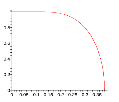
Figure 1: The Hagedorn temperature $T_{H}$ as function of $\Omega$ in the case $(\Omega_{1},\Omega_{2},\Omega_{3})=(\Omega,0,0)$.

For the case $(\Omega_{1},\Omega_{2},\Omega_{3})=(\Omega,0,0)$ depicted in Figure 1 we see that the behavior near the critical point $(T,\Omega)=(0,1)$ is

$$T_{H}(\Omega)=-\frac{1}{\log(1-\Omega)}\left[1-\frac{\log(-\log(1-\Omega))}{\log(1-\Omega)}+\cdots\right]$$ (2.11)

for $1-\Omega\ll 1$. Thus, the slope of the Hagedorn curve in the $(T,\Omega)$ diagram is zero in the critical point $(T,\Omega)=(0,1)$, as is also clear from Figure 1.

     

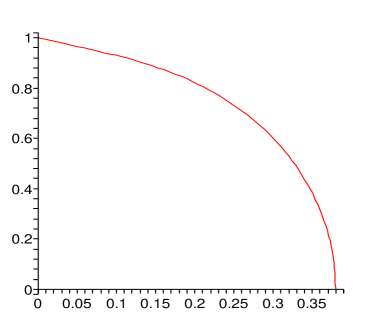
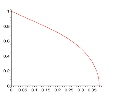
Figure 2: The Hagedorn temperature $T_{H}$ as function of $\Omega$ in the two cases $(\Omega_{1},\Omega_{2},\Omega_{3})=(\Omega,\Omega,0)$, displayed on the left, and $(\Omega_{1},\Omega_{2},\Omega_{3})=(\Omega,\Omega,\Omega)$, displayed on the right.

For the case $(\Omega_{1},\Omega_{2},\Omega_{3})=(\Omega,\Omega,0)$ depicted in the left part of Figure 2 we have instead that the behavior near the critical point $(T,\Omega)=(0,1)$ is

$$T_{H}(\Omega)=\frac{1-\Omega}{\log 2}\left[1-\frac{2}{\log 2}e^{-\frac{1}{2}\log 2/(1-\Omega)}+\mathcal{O}(e^{-\log 2/(1-\Omega)})\right]$$ (2.12)

for $1-\Omega\ll 1$. We see from this that the slope of the Hagedorn curve at the critical point $(T,\Omega)=(0,1)$ is $-\log 2$.

Finally for the case $(\Omega_{1},\Omega_{2},\Omega_{3})=(\Omega,\Omega,\Omega)$ depicted in the right part of Figure 2 we have that the behavior near the critical point $(T,\Omega)=(0,1)$ is

$$T_{H}(\Omega)=\frac{1-\Omega}{\log 4}\left[1-\frac{6}{\log 4}e^{-\log 4/(1-\Omega)}+\mathcal{O}(e^{-2\log 4/(1-\Omega)})\right]$$ (2.13)

for $1-\Omega\ll 1$. We see from this that the slope of the Hagedorn curve at the critical point $(T,\Omega)=(0,1)$ is $-\log 4$.

2.3 Decoupling for near-critical chemical potentials

We now turn to examine what happens when the chemical potentials are near-critical, i.e. when one or more of the chemical potentials $\Omega_{i}$ are close to 1. From Figure 1 and Figure 2 we see that to zoom in to a region where the chemical potentials are near-critical we also need to send the temperature to zero. For $x\rightarrow 0$ it is clear that $z(x,y_{i})\rightarrow 0$ unless we send one or more of the $y_{i}$ to infinity (we restrict ourselves here to positive chemical potentials without loss of generality). Write now $y_{i}=y^{\alpha_{i}}$ where $\alpha_{i}$, $i=1,2,3$, are numbers. Assume without loss of generality $0\leq\alpha_{3}\leq\alpha_{2}\leq\alpha_{1}=1$. From Eq. (2.3) we see then that we should take the limit

$$x\rightarrow 0\ ,\ \ xy=\mbox{fixed}$$ (2.14)

One can now see that we get three different limits depending on if one, two or three of the $\alpha_{i}$, $i=1,2,3$, are equal to one. It is easy to see that this corresponds to sending either one, two or three of the $\Omega_{i}$, $i=1,2,3$, to $1$ as $T\rightarrow 0$. We can therefore restrict ourselves in the following to the three cases $(\alpha_{1},\alpha_{2},\alpha_{3})\in\{(1,0,0),(1,1,0),(1,1,1)\}$.

Writing $y=\exp(\beta\Omega)$ we see that the limit (2.14) means that $T\rightarrow 0$ and $\Omega\rightarrow 1$ such that $T/(1-\Omega)$ is fixed. In fact, it is useful to define

$$\tilde{T}\equiv\frac{T}{1-\Omega}\ ,\ \ \tilde{x}\equiv xy\ ,\ \ \tilde{x}=\exp(-1/\tilde{T})$$ (2.15)

As we shall see, $\tilde{T}$ can be thought of as a temperature in the decoupled sector after taking the limit (2.14). The R-charge that corresponds to the chemical potential $\Omega$ is $R=\sum_{i=1}^{3}\alpha_{i}R_{i}$. With this, we have $y_{1}^{R_{1}}y_{2}^{R_{2}}y_{3}^{R_{3}}=y^{R}$.

Case I: $R=R_{1}$. The half-BPS sector

We take $(\alpha_{1},\alpha_{2},\alpha_{3})=(1,0,0)$ and hence $R=R_{1}$. From the letter partition function (2.3) we see that in the limit (2.14) we have

$$z(x,y_{i})=xy=\tilde{x}$$ (2.16)

up to corrections of order $x$. Therefore, we see that the set of possible letters reduces to just the single letter $Z$, which is the complex scalar in $\mathcal{N}=4$ SYM with weight $(1,0,0)$. The multi-trace operators in this sector are of the form

$$\mathop{{\rm Tr}}(Z^{L_{1}})\mathop{{\rm Tr}}(Z^{L_{2}})\cdots\mathop{{\rm Tr}}(Z^{L_{k}})$$ (2.17)

Thus, the limit we are considering corresponds to being in the well-known half-BPS sector of $\mathcal{N}=4$ SYM spanned by operators of the form (2.17). All the operators of the form (2.17) are chiral primaries of $\mathcal{N}=4$ SYM and preserve at least half of the supersymmetries. By considering the partition function (2.6) for any $N$ we see that the partition function of $U(N)$ $\mathcal{N}=4$ SYM on $\mathbb{R}\times S^{3}$ reduces to the one of the half-BPS sector given by (2.17). The limit thus reduces the $\mathcal{N}=4$ SYM to the quantum mechanical theory with (2.17) as the states in the Hilbert space. This was previously discussed in [17].

If we consider the thermodynamics of the half-BPS sector (2.17) for large $N$ it is easy to see from (2.16) that we never reach the Hagedorn singularity: $\tilde{T}$ can be arbitrarily large.

We note here that the half-BPS sector (2.17) is interesting for various reasons; it contains the states dual to the vacuum of the maximally supersymmetric pp-wave [13, 14], to $AdS_{5}\times S^{5}$ [15], and to giant gravitons in $AdS_{5}\times S^{5}$ [16], and a correspondence between states in this sector and half-BPS backgrounds of type IIB string theory has been found in [12].

Case II: $R=R_{1}+R_{2}$. The $SU(2)$ sector

For this case we take $(\alpha_{1},\alpha_{2},\alpha_{3})=(1,1,0)$ so that $R=R_{1}+R_{2}$ and $(\Omega_{1},\Omega_{2},\Omega_{3})=(\Omega,\Omega,0)$. Taking the limit (2.14) the letter partition function (2.3) now becomes

$$z(x,y_{i})=2xy=2\tilde{x}$$ (2.18)

up to corrections of order $x$. In this case, the set of possible letters reduces to the two complex scalars $Z$ and $X$ with weights $(1,0,0)$ and $(0,1,0)$, respectively. This is due to the fact that these two letters are the only letters for which the conformal dimension is equal to the eigenvalue of $R=R_{1}+R_{2}$. For all other letters the conformal dimension is greater than the eigenvalue of $R$. Thus, the set of multi-operators consist of all operators of the form

$$\mathop{{\rm Tr}}(A^{(1)}_{1}A^{(1)}_{2}\cdots A^{(1)}_{L_{1}})\mathop{{\rm Tr}}(A^{(2)}_{1}A^{(2)}_{2}\cdots A^{(2)}_{L_{2}})\cdots\mathop{{\rm Tr}}(A^{(k)}_{1}A^{(k)}_{2}\cdots A^{(k)}_{L_{k}})\ ,\ \ A^{(i)}_{j}=Z,X$$ (2.19)

From (2.6) we see that the partition function for free $U(N)$ $\mathcal{N}=4$ SYM on $\mathbb{R}\times S^{3}$ in the limit (2.14) is

$$Z(x,y_{i})=\int[dU]\exp\left[\sum_{k=1}^{\infty}\frac{2\tilde{x}^{k}}{k}\mathop{{\rm Tr}}(U^{k})\mathop{{\rm Tr}}((U^{\dagger})^{k})\right]$$ (2.20)

As for the half-BPS sector we see that $\mathcal{N}=4$ SYM in the limit (2.14) is reduced to a quantum mechanical theory, with the multi-trace operators (2.19) as the Hilbert-space. It is not hard to see that precisely the fact that $x\rightarrow 0$ means that the more covariant derivatives an operator has the more decoupled it becomes. Thus, we remove all the modes coming from having a field theory on a space, i.e. in this case the Kaluza-Klein modes on $S^{3}$. In this sense we lose the locality of the field theory and the system becomes instead quantum mechanical.

In Appendix A we take the limit (2.14) in the oscillator representation of $\mathcal{N}=4$ SYM. This is an alternative way of showing that we get the $SU(2)$ sector in the limit (2.14).

For $N=\infty$ it is easy to see from (2.18) that we have a Hagedorn singularity for $\tilde{x}=\frac{1}{2}$, which corresponds to

$$\tilde{T}_{H}=\frac{T_{H}(\Omega)}{1-\Omega}=\frac{1}{\log 2}$$ (2.21)

We note that this precisely corresponds to the leading part of (2.12). Indeed, viewing the limit (2.14) as zooming into the region $T\ll 1$ and $1-\Omega\ll 1$ we see that corresponds to the linear slope of the Hagedorn curve near the critical point $(T,\Omega)=(0,1)$ in the left part of Figure 2.

In conclusion, we see that the $SU(2)$ sector captures the leading features of $\mathcal{N}=4$ SYM on $\mathbb{R}\times S^{3}$ near the critical point $(T,\Omega)=(0,1)$. We also see that despite the fact that $\mathcal{N}=4$ SYM reduces from a field theory to a quantum mechanical theory we keep the interesting physics such as the Hagedorn transition for large $N$. Finally we note that using the partition function (2.20) when $T\ll 1$ and $1-\Omega\ll 1$ instead of the full partition function (2.6) for free $\mathcal{N}=4$ SYM on $\mathbb{R}\times S^{3}$ is a very good approximation. Indeed, if $\Omega=0.99$, the correction on the Hagedorn temperature is of order $10^{-15}$.

Case III: $R=R_{1}+R_{2}+R_{3}$. The $SU(2|3)$ sector

This case has $(\alpha_{1},\alpha_{2},\alpha_{3})=(1,1,1)$ and hence $R=R_{1}+R_{2}+R_{3}$. Taking the limit (2.14) the letter partition function (2.3) reduces to

$$z(x,y_{i})=3xy+2(xy)^{\frac{3}{2}}=3\tilde{x}+2\tilde{x}^{\frac{3}{2}}$$ (2.22)

up to corrections of order $x$. Thus, the set of possible letters reduces to the three complex scalars $Z$, $X$ and $W$ with weights $(1,0,0)$, $(0,1,0)$ and $(0,0,1)$, respectively, and two complex fermions $\chi_{1}$ and $\chi_{2}$ both of weight $(\frac{1}{2},\frac{1}{2},\frac{1}{2})$. This is precisely the $SU(2|3)$ sector of $\mathcal{N}=4$ SYM as defined in [8, 11]. In Appendix A we have shown this using the oscillator representation of $\mathcal{N}=4$ SYM. In this way we show directly that we obtain the $SU(2|3)$ sector as it is defined in [8] in terms of the oscillator representation of $\mathcal{N}=4$ SYM.

The Hilbert space of the $SU(2|3)$ sector consists of the multi-trace operators

$$\begin{array}[]{c}\displaystyle\mathop{{\rm Tr}}(A^{(1)}_{1}A^{(1)}_{2}\cdots A^{(1)}_{L_{1}})\mathop{{\rm Tr}}(A^{(2)}_{1}A^{(2)}_{2}\cdots A^{(2)}_{L_{2}})\cdots\mathop{{\rm Tr}}(A^{(k)}_{1}A^{(k)}_{2}\cdots A^{(k)}_{L_{k}})\\[5.69054pt] \displaystyle A^{(i)}_{j}=Z,X,W,\chi_{1},\chi_{2}\end{array}$$ (2.23)

From (2.6) we see that the partition function for free $U(N)$ $\mathcal{N}=4$ SYM on $\mathbb{R}\times S^{3}$ in the limit (2.14) is

$$Z(x,y_{i})=\int[dU]\exp\left[\sum_{k=1}^{\infty}\frac{3\tilde{x}^{k}+2(-1)^{k+1}\tilde{x}^{\frac{3}{2}k}}{k}\mathop{{\rm Tr}}(U^{k})\mathop{{\rm Tr}}((U^{\dagger})^{k})\right]$$ (2.24)

For $N=\infty$ we see from (2.22) that the Hagedorn singularity occurs at

$$\tilde{T}_{H}=\frac{T_{H}(\Omega)}{1-\Omega}=\frac{1}{\log 4}$$ (2.25)

2.4 Above the Hagedorn temperature

In this section we consider the behavior of free $\mathcal{N}=4$ SYM on $\mathbb{R}\times S^{3}$ above the Hagedorn temperature, following [4]. Since the $N=\infty$ partition function is singular at the Hagedorn temperature we should instead use the exact partition function (2.6) which takes non-trivial relations between multi-trace operators into account. Now, the eigenvalues of the $U(N)$ group element $U$ are elements $e^{i\theta}$ on the unit circle. For large $N$ these eigenvalues become a continuous distribution and we write $\rho(\theta)$ for the density of eigenvalues at the angle $\theta$ normalized such that $\int_{-\pi}^{\pi}d\theta\rho(\theta)=1$. Using this, we find from (2.6) the effective action for the eigenvalues [4]

$$I=N^{2}\sum_{n=1}^{\infty}|\rho_{n}|^{2}a_{n}\ ,\ \ a_{n}(x,y_{i})=\frac{1-z(\omega^{n+1}x^{n},y_{i}^{n})}{n}$$ (2.26)

with $\rho_{n}=\int_{-\pi}^{\pi}d\theta\cos(n\theta)\rho(\theta)$. To find the correct eigenvalue distribution we should minimize $I$. For temperatures below the Hagedorn temperature we have that $a_{n}>0$ and hence the minimum distribution of eigenvalues is the uniform distribution. This is easily seen to give the $N=\infty$ partition function (2.5) [4].

When we reach the Hagedorn temperature we have that $a_{1}=0$, and this means that the minimum of $I$ appears for a non-uniform distribution of the eigenvalues when we are above the Hagedorn temperature. Using the same procedure as in [4] we determine the behavior of the free energy near the transition as a perturbative expansion in $\Delta T\equiv T-T_{H}(\Omega_{i})$ when we are slightly above the Hagedorn temperature. Following [4], the expression for the partition function can be written as

$$-\frac{\log Z}{N^{2}}=-\frac{\epsilon^{2}}{4}-\frac{\epsilon^{3}}{3}-\epsilon^{4}\left(\frac{3}{8}-\frac{1}{4}\sum_{n=2}^{\infty}\frac{n(n^{2}-1)z(x^{n},y_{i}^{n})}{1-z(x^{n},y_{i}^{n})}\right)+{\cal{O}}(\epsilon^{5})$$ (2.27)

where $\epsilon=\cos^{2}(\theta_{0}/2)$, the angle $\theta_{0}$ is defined by $\sin^{2}(\theta_{0}/2)=1-\sqrt{1-1/z(x,y_{i})}$ and $z(x,y_{i})$ is given in Eq. (2.3). The Gibbs free energy $F=F(T,\Omega_{i})$ slightly above the Hagedorn temperature is then given by

$$\frac{F}{N^{2}}=-\frac{1}{4}\left.\frac{\partial z(x,y_{i})}{\partial T}\right|_{T=T_{H}}T_{H}\Delta T-\frac{1}{3}\left(\left.\frac{\partial z(x,y_{i})}{\partial T}\right|_{T=T_{H}}\right)^{3/2}T_{H}\Delta T^{3/2}+{\cal{O}}(\Delta T^{2})$$ (2.28)

with $\Delta T\equiv T-T_{H}(\Omega_{i})\geq 0$. Using (2.28) with (2.10) we get the explicit expansion

$$\begin{array}[]{rcl}\displaystyle\frac{F}{N^{2}}&=&\displaystyle-\beta_{0}\frac{3}{8}\left(1-\beta_{0}\frac{(2\sqrt{3}+\beta_{0})}{36}\sum_{i=1}^{3}\Omega_{i}^{2}+\mathcal{O}(\Omega_{i}^{4})\right)\Delta T\\[11.38109pt] &&\displaystyle-\beta_{0}^{2}\sqrt{\frac{3}{8}}\left(1-\beta_{0}\frac{(4+\sqrt{3}\,\beta_{0})}{24\sqrt{3}}\sum_{i=1}^{3}\Omega_{i}^{2}+\mathcal{O}(\Omega_{i}^{4})\right)\Delta T^{3/2}+{\cal{O}}(\Delta T^{2})\end{array}$$ (2.29)

for $0\leq\Delta T\ll 1$. When the chemical potentials are set to zero we recover the result of [4].

Note from the above that while $F/N^{2}$ in the large $N$ limit is finite for temperatures above the Hagedorn temperature, it is zero for temperatures below the Hagedorn temperature. Thus, we can regard $F/N^{2}$ as an order parameter for the Hagedorn phase transition. Since the derivative of the free energy is discontinuous at the Hagedorn temperature we see that free $U(N)$ $\mathcal{N}=4$ SYM on $\mathbb{R}\times S^{3}$ has a first order phase transition at the Hagedorn temperature [4].

We now turn to the behavior of the free energy slightly above the Hagedorn temperature in the case of near-critical chemical potential. We examine the two cases corresponding to $(\Omega_{1},\Omega_{2},\Omega_{3})=(\Omega,\Omega,0)$ and $(\Omega_{1},\Omega_{2},\Omega_{3})=(\Omega,\Omega,\Omega)$ sending $\Omega\rightarrow 1$ by taking the limit (2.14) described in Section 2.3. In this limit we get a rescaled temperature $\tilde{T}=T/(1-\Omega)$ as defined in (2.15). From this we see that we naturally get a rescaled free energy $\tilde{F}=-\tilde{T}\log Z=F/(1-\Omega)$ where $F$ is the Gibbs free energy. In the limit $\Omega\rightarrow 1$ with $\tilde{T}$ fixed, we get that $\tilde{F}=\tilde{F}(\tilde{T})$, i.e. the rescaled free energy depends only on $\tilde{T}$.

Considering the case $(\Omega_{1},\Omega_{2},\Omega_{3})=(\Omega,\Omega,0)$ we have from Section 2.3 that free $\mathcal{N}=4$ SYM decouples to the $SU(2)$ sector (2.19) in the limit $\Omega\rightarrow 1$ with $\tilde{T}$ fixed. From (2.21) we have that the Hagedorn temperature is $\tilde{T}_{H}=1/\log 2$. Using (2.28), it is straightforward to show that the free energy slightly above the Hagedorn temperature is

$$\frac{\tilde{F}}{N^{2}}=-\frac{\log{2}}{4}(\tilde{T}-\tilde{T}_{H})-\frac{(\log{2})^{2}}{3}(\tilde{T}-\tilde{T}_{H})^{3/2}+{\cal{O}}((\tilde{T}-\tilde{T}_{H})^{2})$$ (2.30)

for $0\leq\tilde{T}-\tilde{T}_{H}\ll 1$. One can either derive this using the full letter partition function (2.3) and then take the limit $\Omega\rightarrow 1$ with $\tilde{T}$ fixed, or alternatively derive it directly using the letter partition function (2.18) for the $SU(2)$ sector.

Similarly we can proceed in the case $(\Omega_{1},\Omega_{2},\Omega_{3})=(\Omega,\Omega,\Omega)$ where we have from Section 2.3 that free $\mathcal{N}=4$ SYM decouples to the $SU(2|3)$ sector (2.23) in the limit $\Omega\rightarrow 1$ with $\tilde{T}$ fixed. We know from Eq. (2.25) that the Hagedorn temperature is $\tilde{T}_{H}=1/\log 4$ and using (2.28) we have that the free energy slightly above the Hagedorn temperature is

$$\frac{\tilde{F}}{N^{2}}=-\frac{9\log 2}{16}(\tilde{T}-\tilde{T}_{H})-\frac{9(\log{2})^{2}}{4\sqrt{2}}(\tilde{T}-\tilde{T}_{H})^{3/2}+{\cal{O}}((\tilde{T}-\tilde{T}_{H})^{2})$$ (2.31)

for $0\leq\tilde{T}-\tilde{T}_{H}\ll 1$. Again, as in the $SU(2)$ sector, this result can be found in two different ways corresponding to either starting from the letter partition function (2.3) and then take the limit on the final result, or starting with the $SU(2|3)$ letter partition function (2.22).

High temperatures

If we consider instead the high temperature regime the eigenvalue distribution becomes almost like a delta-function [4]. Therefore, $\rho_{n}=1$ and we get that $I=N^{2}\sum_{n=1}^{\infty}a_{n}$. If we consider a high-temperature limit with the chemical potentials being fixed, we get the Gibbs free energy

$$F=-\frac{\pi^{2}}{6}V(S^{3})N^{2}T^{4}+\mathcal{O}(T^{3})$$ (2.32)

This is precisely the free energy of free $\mathcal{N}=4$ SYM, i.e. it is the result that one would get from $N^{2}$ times the free energy of $U(1)$ $\mathcal{N}=4$ SYM. Thus while free $\mathcal{N}=4$ SYM on $\mathbb{R}\times S^{3}$ behaves as a confined theory for low temperature, it behaves as a deconfined theory at high temperatures [2, 4].

If we instead consider the case in which $\Omega_{i}/T$ does not go to zero for $T\rightarrow\infty$ for at least one of the chemical potentials, we get the free energy

$$F=-V_{S^{3}}N^{2}\left[\frac{\pi^{2}}{6}T^{4}+\frac{1}{4}T^{2}\sum_{i=1}^{3}\Omega_{i}^{2}-\frac{1}{32\pi^{2}}\left(\sum_{i=1}^{3}\Omega_{i}^{4}-2\sum_{i<j}\Omega_{i}^{2}\Omega_{j}^{2}\right)\right]+{\cal O}(T^{3})$$ (2.33)

This is the same result as in [22, 23] where the free energy is computed as $N^{2}$ times the free energy of free $U(1)$ $\mathcal{N}=4$ SYM. Note that the regularization procedure for obtaining (2.33) is the same as in [22, 23].

3 Quantum mechanical sectors for near-critical chemical potential

In Section 2.3 we saw for free $\mathcal{N}=4$ SYM on $\mathbb{R}\times S^{3}$ that regions with small temperature and near-critical chemical potential are very interesting since the free $\mathcal{N}=4$ SYM effectively reduces to free quantum mechanical systems in such regions. In this section we continue to examine these quantum mechanical sectors of thermal $\mathcal{N}=4$ SYM on $\mathbb{R}\times S^{3}$ but now in the full interacting theory. We show in the following that the interacting $\mathcal{N}=4$ SYM on $\mathbb{R}\times S^{3}$ reduces to well-defined interacting quantum mechanical systems in such regions of small temperature and near-critical chemical potential.

Consider the partition function

$$Z(\beta,\Omega)={\mathop{{\rm Tr}}}_{M}\left(e^{-\beta D+\beta\Omega R}\right)$$ (3.1)

Here $D$ is the dilatation operator of $\mathcal{N}=4$ on $\mathbb{R}\times S^{3}$ which for weak coupling $\lambda\ll 1$ can be expanded as [7, 24]

$$D=D_{0}+\sum_{n=2}^{\infty}\lambda^{n/2}D_{n}$$ (3.2)

where we define for convenience the ’t Hooft coupling as

$$\lambda=\frac{g_{\mathrm{YM}}^{2}N}{4\pi^{2}}$$ (3.3)

Furthermore, $R$ is a linear combination of the three R-charges $R_{1}$, $R_{2}$ and $R_{3}$, with $\Omega$ as the corresponding chemical potential. We restrict in the following to the three cases $R=R_{1}$, $R=R_{1}+R_{2}$ and $R=R_{1}+R_{2}+R_{3}$. Clearly we have that $D_{0}\geq R$ for the three choices of $R$.

We can rewrite the partition function (3.1) as follows

$$Z(\beta,\Omega)={\mathop{{\rm Tr}}}_{M}\left(\exp\left[-\beta(D_{0}-R)-\beta(1-\Omega)R-\beta\lambda D_{2}-\beta\sum_{n=3}^{\infty}\lambda^{n/2}D_{n}\right]\right)$$ (3.4)

Consider the region

$$T\ll 1\ ,\ \ 1-\Omega\ll 1\ ,\ \ \lambda\ll 1$$ (3.5)

We now argue that one can neglect all states with $D_{0}-R>0$ in the partition function (3.4). First we observe that since $\beta\gg 1$ and $D_{0}-R$ is a non-negative integer the states with $D_{0}-R>0$ would have an exceedingly small weight factor. However, one should also ensure then that the $D_{0}=R$ states does not have an equally small weight factor. This is precisely ensured by having $1-\Omega$ and $\lambda\ll 1$. We can therefore write the partition function (3.1) in the region (3.5) as

$$Z(\beta,\Omega)={\mathop{{\rm Tr}}}_{\mathcal{H}}\left(\exp\left[-\beta(1-\Omega)D_{0}-\beta\lambda D_{2}-\beta\sum_{n=3}^{\infty}\lambda^{n/2}D_{n}\right]\right)$$ (3.6)

with

$$\mathcal{H}=\left\{\alpha\in M\Big{|}(D_{0}-R)\alpha=0\right\}$$ (3.7)

i.e. we have restricted the trace to be only over states with $D_{0}=R$. Comparing this to Section 2.3, we see that restricting to states in $\mathcal{H}$ corresponds to the reduction of $\mathcal{N}=4$ SYM on $\mathbb{R}\times S^{3}$ found in the free theory. Defining

$$\tilde{\beta}=\beta(1-\Omega)\ ,\ \ \tilde{\lambda}=\frac{\lambda}{1-\Omega}$$ (3.8)

we can write (3.6) as

$$Z(\tilde{\beta})={\mathop{{\rm Tr}}}_{\mathcal{H}}\left(e^{-\tilde{\beta}H}\right)$$ (3.9)

with $H$ being the Hamiltonian

$$H=D_{0}+\tilde{\lambda}D_{2}+\tilde{\lambda}\sqrt{\lambda}\sum_{n=0}^{\infty}\lambda^{n/2}D_{n+3}$$ (3.10)

Considering the three cases $R=R_{1}$, $R=R_{1}+R_{2}$ and $R=R_{1}+R_{2}+R_{3}$ we have from Section 2.3 that $\mathcal{H}$ in those three cases corresponds to the half-BPS-sector given by (2.17), the $SU(2)$ sector given by (2.19) and the $SU(2|3)$ sector given by (2.23). We have thus shown that interacting $\mathcal{N}=4$ SYM on $\mathbb{R}\times S^{3}$ reduces to those sectors in the region (3.5) with the Hamiltonian given by (3.10).

Note that we have not assumed anything about $N$, thus the above considerations work equally well for finite $N$ and in the large $N$ limit. If we assume $N=\infty$, we can ignore the non-trivial relations between multi-trace operators and work instead with single-trace operators. We can then think of the Hamiltonian (3.10) as the Hamiltonian of a periodic one-dimensional spin-chain. Below we consider the three possible cases and identify the spin-chain models.

Case I: $R=R_{1}$. The half-BPS sector

For $R=R_{1}$ the interacting thermal $\mathcal{N}=4$ SYM on $\mathbb{R}\times S^{3}$ is reduced to the Hamiltonian (3.10) acting on the multi-trace operators of the form (2.17). Since these operators are chiral primaries of $\mathcal{N}=4$ SYM all the interaction terms are zero on these states, and hence the Hamiltonian (3.10) is $H=D_{0}$ for this sector.

Case II: $R=R_{1}+R_{2}$. The $SU(2)$ sector

With $R=R_{1}+R_{2}$ the interacting thermal $\mathcal{N}=4$ SYM on $\mathbb{R}\times S^{3}$ is reduced to a quantum mechanical theory with Hamiltonian (3.10) acting on the $SU(2)$ sector of $\mathcal{N}=4$ SYM on $\mathbb{R}\times S^{3}$ which is spanned by operators of the form (2.19). Note that in the $SU(2)$ sector the half-integer powers of $\lambda$ in (3.10) are not present and we have instead a Hamiltonian of the form [7]

$$H=D_{0}+\tilde{\lambda}D_{2}+\tilde{\lambda}\lambda\sum_{n=0}^{\infty}\lambda^{n}D_{2n+4}$$ (3.11)

For $N=\infty$ we can restrict ourselves to consider the single-trace operators, since they are a well-defined subset of the operators. In the $SU(2)$ sector the single-trace operators are of the form

$$\mathop{{\rm Tr}}(A_{1}A_{2}\cdots A_{L})\ ,\ \ A_{i}\in\{X,Z\}$$ (3.12)

Such single-trace operators can be regarded as spin-chains. In particular a single-trace of length $L$ corresponds to a periodic spin chain of length $L$. For a chain of length $L$ the leading interaction term $D_{2}$ in the Hamiltonian (3.11) is given by [6, 7]

$$D_{2}=\frac{1}{2}\sum_{i=1}^{L}(I_{i,i+1}-P_{i,i+1})$$ (3.13)

Here $P_{i,i+1}$ is the permutation operator and $I_{i,i+1}$ is the identity operator acting on the letters at positions $i$ and $i+1$. This term of the Hamiltonian (3.11) corresponds precisely to the Hamiltonian of the ferromagnetic $XXX_{1/2}$ Heisenberg spin chain reviewed in Appendix B, where we think of the letters $Z$ and $X$ as spin up and spin down. Some of the higher terms in (3.11) are known as well [7, 10], but as will be clear in the following they will not play a role for our considerations since they are much weaker coupled than the $D_{2}$ term. Finally we note that there is considerable evidence that the Hamiltonian (3.11) is integrable [6, 7, 9, 10].

For $N=\infty$ we can thus conclude that the thermodynamics of $\mathcal{N}=4$ SYM on $\mathbb{R}\times S^{3}$ in the region (3.5) with $R=R_{1}+R_{2}$ can be understood from the thermodynamics of the $XXX_{1/2}$ Heisenberg spin chain.

Case III: $R=R_{1}+R_{2}+R_{3}$. The $SU(2|3)$ sector

For the case $R=R_{1}+R_{2}+R_{3}$ the interacting thermal $\mathcal{N}=4$ SYM on $\mathbb{R}\times S^{3}$ in the region (3.5) reduces to a quantum mechanical theory with Hamiltonian (3.10) acting on the $SU(2|3)$ sector of $\mathcal{N}=4$ SYM spanned by operators of the form (2.23).

When $N=\infty$ we can again restrict to the single-trace operators which in this sectors are of the form

$$\mathop{{\rm Tr}}(A_{1}A_{2}\cdots A_{L})\ ,\ \ A_{i}\in\{X,Z,W,\chi_{1},\chi_{2}\}$$ (3.14)

Then a single-trace operator of length $L$ can be regarded as a periodic spin-chain of length $L$. The leading interaction term $D_{2}$ in the Hamiltonian (3.10) can then be written as [8, 11]

$$D_{2}=\frac{1}{2}\sum_{i=1}^{L}(I_{i,i+1}-\Pi_{i,i+1})$$ (3.15)

where $\Pi_{i,i+1}$ is the graded permutation operator which permutes the fields at sites $i$ and $i+1$ picking up a minus sign if the exchange involves two fermions.

In conclusion we have found that for $N=\infty$ the thermodynamics of $\mathcal{N}=4$ SYM on $\mathbb{R}\times S^{3}$ in the region (3.5) with $R=R_{1}+R_{2}+R_{3}$ can be understood from the thermodynamics of the $SU(2|3)$ spin chain with Hamiltonian (3.15).

4 Low temperature limit and the Heisenberg spin chain

In this section we consider what happens as we approach the critical point $(T,\Omega)=(0,1)$ in the specific case of the $SU(2)$ model, i.e. the case with $R=R_{1}+R_{2}$.

We saw in Section 3 that the thermal partition function of $\mathcal{N}=4$ SYM on $\mathbb{R}\times S^{3}$ in the region (3.5) with $R=R_{1}+R_{2}$ reduces to the partition function (3.9) with the Hamiltonian (3.11). For $N=\infty$ we have that a single-trace of fixed length $L$ corresponds to periodic spin-chain of length $L$ and the Hamiltonian (3.11) is a spin-chain Hamiltonian, with the leading interaction term $D_{2}$ corresponding to an $XXX_{1/2}$ Heisenberg spin chain Hamiltonian.

Consider now being in the region (3.5). Take then the zero temperature limit $T\rightarrow 0$ keeping $\lambda$ and $\tilde{T}=T/(1-\Omega)$ fixed. In the $(T,\Omega)$ diagram depicted in the left part of Figure 2 this corresponds to moving towards the critical point $(T,\Omega)=(0,1)$ in a straight line with slope $1/\tilde{T}$. In terms of the partition function (3.9) and Hamiltonian (3.11) we see that this corresponds to fixing the temperature while increasing the $\tilde{\lambda}$ coupling. Since we have that $\lambda\ll 1$ and since $\tilde{\lambda}$ is growing towards infinity, we can ignore the higher terms in (3.11) and instead work with the Hamiltonian

$$H=D_{0}+\tilde{\lambda}D_{2}$$ (4.1)

with $D_{2}$ given by (3.13). For a fixed length $L$ of the chain (or for the single-trace operators) this is precisely the ferromagnetic $XXX_{1/2}$ Heisenberg spin chain Hamiltonian (plus a constant term). Therefore, we see that the approach to the critical point $(T,\Omega)=(0,1)$ is governed completely by the $XXX_{1/2}$ Heisenberg spin chain. Note that letting $\tilde{\lambda}$ go to infinity does not spoil our approximations of Section 3 since we always have that $\beta\gg\tilde{\beta}$.

Since we are keeping $\tilde{\beta}$ fixed we see from the weight factor $e^{-\tilde{\beta}L-\tilde{\beta}\tilde{\lambda}D_{2}}$ that it is reasonable to consider the limit for a chain of fixed length since the coupling in front of $L$ is constant. The remaining part of the weight factor is $e^{-\tilde{\beta}\tilde{\lambda}D_{2}}$ and thus we see that our limit corresponds to taking the zero temperature limit of the $XXX_{1/2}$ Heisenberg spin chain.

As reviewed in Appendix B we have that the states with the lowest energy of the ferromagnetic $XXX_{1/2}$ Heisenberg spin chain are the zero eigenvalue states of $D_{2}$, which when written as single-trace operators are of the form

$$\mathop{{\rm Tr}}\left(\mbox{sym}(Z^{L-M}X^{M})\right)$$ (4.2)

where ’sym’ means total symmetrization. It is clear that any state which is totally symmetrized has eigenvalue one under the permutation operator, hence the eigenvalue of $D_{2}$ is zero on such states. Since $0\leq M\leq L$ we have $L+1$ different vacuum states for a chain of length $L$. Now, since our limit corresponds to taking the zero temperature limit of the $XXX_{1/2}$ Heisenberg spin chain, and since the zero temperature limit means that the states with lowest energy dominates, we can conclude that we are driven towards the vacuum states (4.2) as we approach the critical point $(T,\Omega)=(0,1)$.

That we are driven towards the states (4.2) makes sense also from another point of view, namely that (4.2) corresponds to chiral primaries of $\mathcal{N}=4$ SYM, and thus the zero temperature limit that we are taking is driving us towards a $1/2$ BPS sector of $\mathcal{N}=4$ SYM.

There is also another zero temperature limit which is natural to consider. Start again in the region (3.5). Let then $T\rightarrow 0$ with $\Omega$ and $\lambda$ being fixed. In this limit we have that the rescaled temperature $\tilde{T}$ decreases, while the couplings $\tilde{\lambda}$ and $\lambda$ both are fixed. This means that this limit corresponds to keeping the Hamiltonian (3.11) fixed while changing the temperature $\tilde{T}$ of the decoupled theory. Thus, in this limit we are moving towards the ground states of the quantum mechanical theory given by the Hamiltonian (3.11). For $N=\infty$ we can consider the single-trace operators of a fixed length. Then the $D_{0}$ term in (3.11) can be ignored and to leading order (neglegting the $D_{4}$ term and higher terms) we have a zero temperature limit of the ferromagnetic $XXX_{1/2}$ Heisenberg spin chain. As for the previous limit considered above, this means we are driven towards the ferromagnetic vacuum states (4.2), which are chiral primaries of $\mathcal{N}=4$ SYM.

We considered in the above two zero temperature limits of the $SU(2)$ sector. It is not hard to see that we get similar results for the corresponding zero temperature limits in the $SU(2|3)$ sector. In particular, we are driven towards the vacuum states of the $SU(2|3)$ spin chain given by (3.15) which are the states that have zero eigenvalue for $D_{2}$. Moreover, these states are chiral primaries of $\mathcal{N}=4$ SYM.

5 Decoupling limit to exact quantum mechanical Hamiltonian

We show in the following that we can take decoupling limits of the thermal interacting $\mathcal{N}=4$ SYM on $\mathbb{R}\times S^{3}$ to a quantum mechanical system which is described exactly by the one-loop corrected Hamiltonian in that sector. For $N=\infty$ the Hamiltonians are the ones of the well-known spin-chain models.

Consider the partition function (3.1) with the full dilatation operator (3.2). We consider here again the cases $R=R_{1}$, $R=R_{1}+R_{2}$ and $R=R_{1}+R_{2}+R_{3}$. Consider then the following decoupling limit

$$T\rightarrow 0\ ,\ \ \tilde{T}\equiv\frac{T}{1-\Omega}\ \mbox{fixed}\ ,\ \ \tilde{\lambda}\equiv\frac{\lambda}{1-\Omega}\ \mbox{fixed}$$ (5.1)

Clearly $\Omega\rightarrow 1$ and $\lambda\rightarrow 0$ in this limit. From the partition function (3.1) it is clear that we can ignore states with $D_{0}>R$, and hence we only have states with $D_{0}=R$. Applying the arguments of Section 3 we get that the limit (5.1) of the full partition function (3.1) reduces to the limit (5.1) of the reduced partition function (3.6). Since $\lambda\rightarrow 0$ we see that all the higher-loop terms drop out, and only the $D_{0}$ and $D_{2}$ terms remain. The limit (5.1) of the partition function (3.1) therefore gives the result

$$Z(\tilde{\beta})={\mathop{{\rm Tr}}}_{\mathcal{H}}\left(e^{-\tilde{\beta}H}\right)$$ (5.2)

where $H$ is the Hamiltonian

$$H=D_{0}+\tilde{\lambda}D_{2}$$ (5.3)

Thus, thermal interacting $\mathcal{N}=4$ SYM on $\mathbb{R}\times S^{3}$ in the limit (5.1) is described exactly by the Hamiltonian (5.3). Note here that this is true for any $N$. Furthermore, it is interesting to note that $\tilde{\lambda}$ can take any value. One can thus end up with a strongly coupled $D_{2}$ term in the Hamiltonian as a good description of $\mathcal{N}=4$ SYM, as we in fact already saw in Section 4.

For $N=\infty$, we get as above that we can think of the single-trace operators as spin-chains. We thus have that the thermodynamics of interacting $\mathcal{N}=4$ SYM on $\mathbb{R}\times S^{3}$ in the decoupling limit (5.1) can be described exactly by a spin-chain model with Hamiltonian (5.3).

If we consider the case $R=R_{1}+R_{2}$ for $N=\infty$ we see that the thermodynamics of $\mathcal{N}=4$ SYM on $\mathbb{R}\times S^{3}$ in the decoupling limit (5.1) can be described exactly by the ferromagnetic $XXX_{1/2}$ Heisenberg spin chain (see Appendix B). This is easily seen from the Hamiltonian (5.3) with $D_{2}$ given in (3.13). Written explicitly, we have that the full partition function for $\mathcal{N}=4$ SYM in the limit (5.1) is

$$\log Z(\tilde{T})=\sum_{n=1}^{\infty}\sum_{L=1}^{\infty}\frac{1}{n}e^{-nL/\tilde{T}}Z^{(XXX)}_{L}(\tilde{T}/n)$$ (5.4)

where $Z^{(XXX)}_{L}$ is the partition function for the ferromagnetic $XXX_{1/2}$ Heisenberg spin chain of length $L$ with Hamiltonian $\tilde{\lambda}D_{2}$.

Similarly, for the case $R=R_{1}+R_{2}+R_{3}$ we have that the thermodynamics of $\mathcal{N}=4$ SYM on $\mathbb{R}\times S^{3}$ in the decoupling limit (5.1) can be described exactly by the spin chain model given by the $D_{2}$ term (3.15).

In conclusion we have found limits in which planar thermal $\mathcal{N}=4$ SYM is described exactly by well-defined spin-chain models. The spin-chain models involved are short-range and the coupling $\tilde{\lambda}$ in front of the spin chain term $D_{2}$ in the Hamiltonian can take any value.

6 One-loop partition function

In this section we consider the one-loop correction to the partition function for $U(N)$ $\mathcal{N}=4$ SYM on $\mathbb{R}\times S^{3}$ with non-zero chemical potentials in planar limit $N=\infty$, generalizing the procedure in [18]. We use this to find the one-loop correction to the Hagedorn temperature. We consider subsequently the one-loop correction to the partition function and Hagedorn temperature for the near-critical regions where $\mathcal{N}=4$ SYM reduces to the $SU(2)$ and $SU(2|3)$ sectors.

One-loop correction to partition function and Hagedorn temperature

Consider the complete single-trace partition function ${Z}_{\rm ST}=\mathop{{\rm Tr}}(x^{D}\prod_{i=1}^{3}y_{i}^{R_{i}})$ for $U(N)$ $\mathcal{N}=4$ SYM on $\mathbb{R}\times S^{3}$ in the planar limit. Up to the first order in the ’t Hooft coupling $\lambda$ the single-trace partition function can be written as ${Z}_{\rm ST}={Z}_{\rm ST}^{(0)}+\lambda{Z}_{\rm ST}^{(1)}+\mathcal{O}(\lambda^{2})$ where ${Z}_{\rm ST}^{(0)}$ is the zeroth order single-trace partition function given in (2.4) and with the first-order contribution given by

$${Z}_{\rm ST}^{(1)}(x,y_{i})=\log x\mathop{{\rm Tr}}\left[\prod_{i=1}^{3}y_{i}^{R_{i}}x^{D_{0}}D_{2}\right]$$ (6.1)

This follows from the expansion (3.2) of the dilatation operator and from the fact that the R-charges commute with the dilatation operator. Applying the arguments of [18] where it is used that one can refrase (6.1) as a spin-chain partition function, we arrive at the following expression for the one-loop single trace partition function

$$\begin{array}[]{rcl}\displaystyle{Z}_{\rm ST}^{(1)}(x,y_{i})&=&\displaystyle\log x\sum_{L=1}^{\infty}\sum_{\tiny\begin{array}[]{c}k=0\\[-2.84526pt] (k,L)=1\end{array}}^{L-1}\left(\frac{\langle D_{2}(\omega^{L+1}x^{L},y_{i}^{L})\rangle}{1-z(\omega^{L+1}x^{L},y_{i}^{L})}\right.\\[19.91692pt] &&\displaystyle+\left.\delta_{L\neq 1}\langle PD_{2}(\omega^{L-k+1}x^{L-k},y_{i}^{(L-k)},\omega^{k+1}x^{k},y_{i}^{k})\rangle\right)\end{array}$$ (6.2)

with

$$\displaystyle\langle D_{2}(x,y_{i})\rangle=\sum_{A_{1},A_{2}\in\mathcal{A}}\prod_{i=1}^{3}x^{d(A_{1})+d(A_{2})}y_{i}^{R_{i}(A_{1})+R_{i}(A_{2})}\langle A_{1}A_{2}|D_{2}|A_{1}A_{2}\rangle$$ (6.3)

$$\displaystyle\langle PD_{2}(w,y_{i},\bar{w},\bar{y}_{i})\rangle=\sum_{A_{1},A_{2}\in\mathcal{A}}\prod_{i=1}^{3}w^{d(A_{1})}y_{i}^{R_{i}(A_{1})}\bar{w}^{d(A_{2})}\bar{y}_{i}^{R_{i}(A_{2})}\langle A_{1}A_{2}|D_{2}|A_{2}A_{1}\rangle$$ (6.4)

Here $L$ can be seen as the length of the spin chain and $(k,L)=1$ means that $k$ and $L$ are relatively prime. We have also included the fermion contribution. We note that Eq. (6.2) is a direct generalization of the result of [18]. From (6.2) it is in principle straightforward to compute the one-loop correction (6.1), once the two expectation values (6.3) and (6.4) are known. From this one gets the corrected multi-trace partition function using the general prescription in (2.5). In Appendix (C) we computed $\langle D_{2}\rangle$ and we sketched how to compute $\langle PD_{2}\rangle$. We have not computed the corrected partition function here explicitly since we do not need it for the purposes of this paper. However, below we compute it explicitly in the near-critical regions giving the $SU(2)$ and $SU(2|3)$ sectors.

We use now the result (6.2) to compute the one-loop correction to the Hagedorn temperature. From Eq. (2.9) we have that the zeroth order contribution to the partition function goes like $(T_{H}-T)^{-1}$ near the Hagedorn temperature, for fixed chemical potentials. This behavior resists also for the corrected partition function where now the value of the Hagedorn temperature is shifted by the higher loop corrections. One can then compute the one-loop corrected Hagedorn temperature by considering the pole of ${Z}_{\rm ST}^{(1)}$ in (6.2) at the zeroth order Hagedorn temperature $T^{(0)}_{H}$. As in the case of zero chemical potentials [18] the term proportional to $\langle PD_{2}\rangle$ does not give rise to divergences. Hence, we get the following formula for the one-loop correction to the Hagedorn temperature

$$\delta T_{H}=\lambda\left.\frac{\langle D_{2}\rangle}{T\frac{\partial z}{\partial T}}\right|_{T=T_{H}^{(0)}}$$ (6.5)

for given chemical potentials $\Omega_{i}$.

Using Eq. (6.5), we compute now the one-loop corrected Hagedorn temperature for small values of the chemical potentials $\Omega_{i}$. To this end, we use the results on $\langle D_{2}\rangle$ of Appendix C to find the following expression for $\langle D_{2}\rangle$ evaluated at the Hagedorn temperature for small chemical potentials

$$\langle D_{2}\rangle = \frac{3}{4}\left[1-\frac{\beta_{0}^{2}}{18}\sum_{i=1}^{3}\Omega_{i}^{2}-\frac{\beta_{0}^{3}}{864}\left(72-56\sqrt{3}+3\beta_{0}(41-26\sqrt{3})\right)\sum_{i<j}\Omega_{i}^{2}\Omega_{j}^{2}\right.$$ (6.7)

$$\left.-\frac{\beta_{0}^{3}}{1296}\left(72-56\sqrt{3}+3\beta_{0}(45-26\sqrt{3})\right)\sum_{i=1}^{3}\Omega_{i}^{4}+\mathcal{O}(\Omega_{i}^{6})\right]$$

To compute this we used the zeroth order Hagedorn temperature for small chemical potentials given in Eq. (2.10). Inserting Eq. (6.7) in Eq. (6.5), we find that the one-loop corrected Hagedorn temperature for small chemical potentials is

$$\begin{array}[]{c}\displaystyle T_{H}(\Omega_{i})=p_{0}+p_{1}\sum_{i=1}^{3}\Omega_{i}^{2}+p_{2}\sum_{i<j}\Omega_{i}^{2}\Omega_{j}^{2}+p_{3}\sum_{i=1}^{3}\Omega_{i}^{4}+\mathcal{O}(\Omega_{i}^{6})\\[14.22636pt] \displaystyle p_{0}=\frac{1}{\beta_{0}}\left(1+\frac{{\lambda}}{2}\right)+\mathcal{O}(\lambda^{2})\ ,\ \ p_{1}=-\frac{1}{6\sqrt{3}}\left(1-\frac{{\lambda}}{2}(11-\beta_{0}\sqrt{3})\right)+\mathcal{O}(\lambda^{2})\\[11.38109pt] \displaystyle p_{2}=\frac{\beta_{0}}{1296}\left[18-5\sqrt{3}+{\lambda}\left(60-\beta_{0}\left(72-35\sqrt{3}-\beta_{0}(69\sqrt{3}-113)\right)\right)\right]+\mathcal{O}(\lambda^{2})\\[11.38109pt] \displaystyle p_{3}=\frac{\beta_{0}}{2592}\left[18-11\sqrt{3}+{\lambda}\left(60-\beta_{0}\left(72-47\sqrt{3}-\beta_{0}(69\sqrt{3}-122)\right)\right)\right]+\mathcal{O}(\lambda^{2})\end{array}$$ (6.8)

Note that for zero chemical potentials in Eqs. (6.7) and (6.8) we recover the result of [18].

The $SU(2)$ sector

We consider now the near-critical region (3.5) with $(\Omega_{1},\Omega_{2},\Omega_{3})=(\Omega,\Omega,0)$. From Section 3 we know that the single-trace sector of the planar limit of $U(N)$ $\mathcal{N}=4$ SYM on $\mathbb{R}\times S^{3}$ reduces to the $SU(2)$ sector with single-traces of the form (3.12). From Section 3 we have furthermore that we can consider $\tilde{T}=T/(1-\Omega)$ as the effective temperature and that the one-loop corrected Hamiltonian becomes $H=D_{0}+\tilde{\lambda}D_{2}$ with $\tilde{\lambda}=\lambda/(1-\Omega)$. In the following we employ these results to find the corrected partition function and Hagedorn temperature for this near-critical region. Note that we assume in the following that $\tilde{\lambda}\ll 1$.

From Section 2 we have that the zeroth order contribution to the partition function for the $SU(2)$ sector is

$$Z^{(0)}_{\rm ST}(\tilde{x})=-\sum_{k=1}^{\infty}\frac{\varphi(k)}{k}\log(1-2\tilde{x}^{k})$$ (6.9)

We now consider the first correction in $\tilde{\lambda}$ to this partition function when $\tilde{\lambda}\ll 1$. To this end, we use the formula [18]

$${Z}_{\rm ST}^{(1)}(\tilde{x})=\log{\tilde{x}}\sum_{L=1}^{\infty}\sum_{\tiny\begin{array}[]{c}k=0\\[-2.84526pt] (k,L)=1\end{array}}^{L-1}\left(\frac{\langle D_{2}(\omega^{L+1}\tilde{x}^{L})\rangle}{1-z(\omega^{L+1}\tilde{x}^{L})}+\delta_{L\neq 1}\langle PD_{2}(\omega^{L-k+1}\tilde{x}^{L-k},\omega^{k+1}\tilde{x}^{k})\rangle\right)$$ (6.10)

In the $SU(2)$ sector the expectation values of $D_{2}$ and $PD_{2}$ are given by [18]

$$\langle D_{2}(\tilde{x})\rangle=\tilde{x}^{2},~{}~{}~{}~{}~{}\langle PD_{2}(\tilde{x}_{1},\tilde{x}_{2})\rangle=-\tilde{x}_{1}\tilde{x}_{2}$$ (6.11)

Substituting now those expressions into the formula (6.10), we recover the known result for the one-loop partition function in the $SU(2)$ sector [18]

$$Z^{(1)}_{\rm ST}(\tilde{x})=\log{\tilde{x}}\left[\tilde{x}-\sum_{n=1}^{\infty}\varphi(n)\tilde{x}^{n}\left(\frac{1-3\tilde{x}^{n}}{1-2\tilde{x}^{n}}\right)\right]$$ (6.12)

Similarly to Eq. (6.5), we have that the correction to the Hagedorn temperature is

$$\delta\tilde{T}_{H}=\tilde{\lambda}\left.\frac{\langle D_{2}\rangle}{\tilde{T}\frac{\partial z(\tilde{x})}{\partial\tilde{T}}}\right|_{\tilde{T}=\tilde{T}^{(0)}_{H}}$$ (6.13)

where $\tilde{T}^{(0)}_{H}=1/\log 2$. We used here that $\langle PD_{2}\rangle$ is not divergent, as one can see from (6.11). From Eqs. (6.11) and (6.13) we get then that the corrected Hagedorn temperature for $\tilde{\lambda}\ll 1$ is

$$\tilde{T}_{H}=\frac{1}{\log{2}}\left(1+\frac{1}{4}\tilde{\lambda}+\mathcal{O}(\tilde{\lambda}^{2})\right)$$ (6.14)

It is important to notice that starting instead from the general expressions for $\langle D_{2}({x},y_{i})\rangle$ and $\langle PD_{2}({x},y_{i})\rangle$ for $\mathcal{N}=4$ SYM given in Appendix C and taking the limit (5.1) precisely gives the result (6.11). From this fact one can in turn see that both the one-loop corrected partition function and Hagedorn temperature reduces to (6.12) and (6.14) found above. This is in accordance with our derivation of the interacting Hamiltonian in Section 3.

Finally we note that the two loop corrected Hagedorn temperature in the $SU(2)$ sector has been considered in [25]. However, their result is not directly applicable in our case, since the two Hamiltonians for the corrections are different.

The $SU(2|3)$ sector

In the $SU(2|3)$ sector the story is very similar to the one for the $SU(2)$ sector. We are considering the near-critical region (3.5) with $(\Omega_{1},\Omega_{2},\Omega_{3})=(\Omega,\Omega,\Omega)$. From Section 3 we know that the single-trace sector of the planar limit of $U(N)$ $\mathcal{N}=4$ SYM on $\mathbb{R}\times S^{3}$ reduces to the $SU(2|3)$ sector with single-traces of the form (3.14). The zeroth order single-trace partition function is

$$Z^{(0)}_{\rm ST}(\tilde{\beta})=-\sum_{k=1}^{\infty}\frac{\varphi(k)}{k}\log\left(1-3\tilde{x}^{k}-2(-1)^{k+1}\tilde{x}^{3k/2}\right)$$ (6.15)

We compute the first correction in $\tilde{\lambda}$ to this partition function when $\tilde{\lambda}\ll 1$ using again Eq. (6.10). Using that the dilatation operator is given by (3.15) we find

$$\begin{array}[]{rcl}\langle D_{2}(\tilde{x})\rangle&=&\displaystyle 3\tilde{x}^{2}+6\tilde{x}^{5/2}+3\tilde{x}^{3}\\[5.69054pt] \langle PD_{2}(\tilde{x}_{1},\tilde{x}_{2})\rangle&=&\displaystyle-3\tilde{x}_{1}\tilde{x}_{2}+3\tilde{x}_{1}^{3/2}\tilde{x}_{2}^{3/2}-3\left[\tilde{x}_{1}^{3/2}\tilde{x}_{2}+\tilde{x}_{1}\tilde{x}_{2}^{3/2}\right]\end{array}$$ (6.16)

As for the $SU(2)$ sector, these results can be recovered using the expressions for $\langle D_{2}({x},y_{i})\rangle$ and $\langle PD_{2}({x},y_{i})\rangle$ for $\mathcal{N}=4$ SYM given in Appendix C and taking the limit (5.1). Inserting the previous expressions in Eq. (6.10) we get that the one-loop partition function in the $SU(2|3)$ sector is given by

$$\begin{array}[]{rcl}\displaystyle{Z}^{(1)}_{\rm{ST}}(\tilde{x})&=&\displaystyle\log{\tilde{x}}\left[3\tilde{x}+3\tilde{x}^{3/2}-3\sum_{L=2}^{\infty}\right.\sum_{\tiny\begin{array}[]{c}k=0\\[-2.84526pt] (k,L)=1\end{array}}^{L-1}\left((-1)^{L-k+1}\tilde{x}^{(3L-k)/2}+(-1)^{k+1}\tilde{x}^{L+k/2}\right)\\[19.91692pt] &&\ \ \ \ \ \ \ \displaystyle\left.-3\sum_{n=1}^{\infty}\varphi(n)\tilde{x}^{n}\frac{1-(-1)^{n}\tilde{x}^{n/2}-4\tilde{x}^{n}+7(-1)^{n}\tilde{x}^{3n/2}-3\tilde{x}^{2n}}{1-3\tilde{x}^{n}-2(-1)^{n+1}\tilde{x}^{3n/2}}\right]\end{array}$$ (6.17)

Using now Eqs. (6.13) and (6.16) we get for the one-loop corrected Hagedorn temperature the following result

$$\tilde{T}_{H}=\frac{1}{\log{4}}\left(1+\frac{3}{8}\tilde{\lambda}+\mathcal{O}(\tilde{\lambda}^{2})\right)$$ (6.18)

One can check that only the $\langle D_{2}(\tilde{x})\rangle$ part of the one-loop partition function contributes to this.

7 Discussion and conclusions

In this paper we have found that thermal $\mathcal{N}=4$ SYM on $\mathbb{R}\times S^{3}$ greatly reduces near the critical points $(T,\Omega_{1},\Omega_{2},\Omega_{3})=(0,1,0,0)$, $(T,\Omega_{1},\Omega_{2},\Omega_{3})=(0,1,1,0)$ and $(T,\Omega_{1},\Omega_{2},\Omega_{3})=(0,1,1,1)$. We identified the three quantum mechanical theories that $\mathcal{N}=4$ SYM reduces to, and in particular we showed that the Hilbert spaces correspond to a half-BPS sector and the $SU(2)$ and $SU(2|3)$ sectors of $\mathcal{N}=4$ SYM. We found the Hamiltonian for these three theories and we saw that the one-loop correction to the dilatation operator has a special significance in this. The existence of these quantum mechanical sectors of $\mathcal{N}=4$ SYM could prove highly useful. Through the AdS/CFT correspondence the thermodynamics of $\mathcal{N}=4$ SYM is linked to the Hagedorn transition in string theory, and since for instance the $SU(2)$ sector is greatly reduced in complexity compared to the full $\mathcal{N}=4$ SYM, we can get a much better handle on the behavior of $\mathcal{N}=4$ SYM in this particular near-critical region than on $\mathcal{N}=4$ SYM with zero chemical potentials.

For $N=\infty$ we found that the near-critical regions giving the $SU(2)$ and $SU(2|3)$ sectors can be described in terms of spin chain theories. In particular the $SU(2)$ sector corresponds to a ferromagnetic $XXX_{1/2}$ Heisenberg spin chain to leading order (or exactly, if we take the limit of Section 5). This provides a very different realization of spin chains for the planar limit of $\mathcal{N}=4$ SYM on $\mathbb{R}\times S^{3}$ than in the study of integrability [6, 7, 9]. In terms of integrability, the $SU(2)$ and $SU(2|3)$ sectors are closed subsectors of the conjectured complete $\mathcal{N}=4$ spin chain, i.e. they decouple to all orders in perturbation theory [11]. However, it is not clear that this decoupling holds at strong coupling [26, 27]. Instead, in the limit of this paper we have an effective reduction of $\mathcal{N}=4$ SYM to the $SU(2)$ and $SU(2|3)$ sectors which does not rely on the $SU(2)$ and $SU(2|3)$ sectors being closed in the sense of having interactions with the other operators of $\mathcal{N}=4$ SYM. Any such interaction would in any case be suppressed in the near-critical regions that we consider. It would therefore be interesting to consider if our decoupling of the $SU(2)$ and $SU(2|3)$ sectors corresponds to a similar decoupling for thermal string theory on ${\rm AdS}_{5}\times S^{5}$ with near-critical chemical potentials.

It is intriguing to compare our limit to the pp-wave limits of ${\rm AdS}_{5}\times S^{5}$ [14]. It is not hard to see that the near-critical region giving us the reduction to the $SU(2)$ sector has some similarities with the pp-wave limit of [28] since we keep only states with $D_{0}=R_{1}+R_{2}$. It is clear that to connect to the limit of $\mathcal{N}=4$ SYM found in [28] we need to consider only a subsector of the pp-wave string theory of [28]. This seems possible to achieve by turning on the appropriate chemical potential. This would be interesting to study since we have a Hagedorn transition both in the gauge theory side and on the pp-wave side [29].

Another interesting direction to pursue would be to compare our results on the Hagedorn temperature as a function of the chemical potential to the Hawking-Page transition [5, 1] with chemical potentials [30]. With the chemical potentials set to zero we have a consistent picture that the Hagedorn transition is a first order transition both for weak coupling $\lambda\ll 1$ [4, 31] and for strong coupling $\lambda\gg 1$ [32] where it is mapped to the Hawking-Page transition. It would be interesting to see whether the picture is equally consistent once the chemical potentials are turned on.

Finally, we note that we expect similar decoupled quantum mechanical sectors in other supersymmetric gauge theories with R-symmetry, in regions with near-critical chemical potentials.

Appendix A Oscillator representation of $\mathcal{N}=4$ SYM

In the oscillator representation of $\mathcal{N}=4$ SYM [33, 8] we can write all the gauge-invariant operators using two bosonic oscillators $\mathbf{a}^{\alpha}$, $\mathbf{b}^{\dot{\alpha}}$, $\alpha,\dot{\alpha}=1,2$, and one fermionic oscillator $\mathbf{c}^{a}$, $a=1,2,3,4$, with the commutation relations

$$\left[\mathbf{a}^{\alpha},{\mathbf{a}}^{\dagger}_{\beta}\right]=\delta^{\alpha}_{\beta}~{}~{}~{}~{}\left[\mathbf{b}^{\dot{\alpha}},{\mathbf{b}}^{\dagger}_{\dot{\beta}}\right]=\delta^{\dot{\alpha}}_{\dot{\beta}}~{}~{}~{}~{}\left\{\mathbf{c}^{a},{\mathbf{c}}^{\dagger}_{b}\right\}=\delta^{a}_{b}$$ (A.1)

In terms of these oscillators, the set of letters $\mathcal{A}$ of $\mathcal{N}=4$ SYM is given by

$$\begin{array}[]{c}\phi\ :\ ({\mathbf{c}}^{\dagger})^{2}|0\rangle\mbox{ repr. }[0,1,0]_{(0,0)}\\[2.84526pt] \psi\ :\ {\mathbf{a}}^{\dagger}{\mathbf{c}}^{\dagger}|0\rangle\mbox{ repr. }[0,0,1]_{(\frac{1}{2},0)}\ ,\ \ \bar{\psi}\ :\ {\mathbf{b}}^{\dagger}({\mathbf{c}}^{\dagger})^{3}|0\rangle\mbox{ repr. }[1,0,0]_{(0,\frac{1}{2})}\\[2.84526pt] F\ :\ ({\mathbf{a}}^{\dagger})^{2}|0\rangle\mbox{ repr. }[0,0,0]_{(1,0)}\ ,\ \ \bar{F}\ :\ ({\mathbf{b}}^{\dagger})^{2}|0\rangle\mbox{ repr. }[0,0,0]_{(0,1)}\\[2.84526pt] D\ :\ {\mathbf{a}}^{\dagger}{\mathbf{b}}^{\dagger}\mbox{ repr. }[0,0,0]_{(\frac{1}{2},\frac{1}{2})}\end{array}$$ (A.2)

where $F$ is the field strength, $\psi$ the fermions and $\phi$ the scalars. Moreover $D$ is the covariant derivative. One can then generate $\mathcal{A}$ by acting with $D^{k}$. Note that we also specified the representation under $SU(4)\times SO(4)$ that the fields are in, for example $[0,0,1]_{(1/2,0)}$ corresponds to the $[0,0,1]$ of $SU(4)$ and the $(\frac{1}{2},0)$ of $SO(4)$.

Write now the number operators as $a^{\alpha}={\mathbf{a}}^{\dagger}_{\alpha}\mathbf{a}^{\alpha}$, $b^{\dot{\alpha}}={\mathbf{b}}^{\dagger}_{\dot{\alpha}}\mathbf{b}^{\dot{\alpha}}$ and $c^{a}={\mathbf{c}}^{\dagger}_{a}\mathbf{c}^{a}$, where it should be understood that there are no sums over the indices. We define then the operators

$$\begin{array}[]{rcl}\displaystyle C&=&\displaystyle 1-\frac{1}{2}(a^{1}+a^{2})+\frac{1}{2}(b^{1}+b^{2})-\frac{1}{2}(c^{1}+c^{2}+c^{3}+c^{4})\\[8.53581pt] \displaystyle D_{0}&=&\displaystyle 1+\frac{1}{2}(a^{1}+a^{2}+b^{1}+b^{2})\end{array}$$ (A.3)

Here $C$ is the central charge which should be annihilated on physical states, while $D_{0}$ is the dilatation operator in free $\mathcal{N}=4$ SYM. The three R-charges are

$$R_{1}=\frac{1}{2}(c^{1}-c^{2}-c^{3}+c^{4})\ ,\ \ R_{2}=\frac{1}{2}(-c^{1}+c^{2}-c^{3}+c^{4})\ ,\ \ R_{3}=\frac{1}{2}(-c^{1}-c^{2}+c^{3}+c^{4})$$ (A.4)

We can now write the letter partition function as

$$\begin{array}[]{l}\displaystyle z(x,y_{1},y_{2},y_{3})={\mathop{{\rm Tr}}}_{\mathcal{A}}\left(x^{D_{0}}y_{1}^{R_{1}}y_{2}^{R_{2}}y_{3}^{R_{3}}\right)=\sum_{a_{1},a_{2},b_{1},b_{2}=0}^{\infty}\sum_{c^{1},c^{2},c^{3},c^{4}=0}^{1}\delta(C)x^{D_{0}}y_{1}^{R_{1}}y_{2}^{R_{2}}y_{3}^{R_{3}}\\[14.22636pt] \displaystyle=\sum_{a,b=0}^{\infty}(a+1)(b+1)\sum_{c^{1},c^{2},c^{3},c^{4}=0}^{1}\delta\Big{(}2-a+b-\sum_{a=1}^{4}c^{a}\Big{)}x^{1+\frac{1}{2}(a+b)}y_{1}^{R_{1}}y_{2}^{R_{2}}y_{3}^{R_{3}}\end{array}$$ (A.5)

It is straightforward to see that this gives the letter partition function (2.3) computed in Section 2.1. Note that we defined $a=a^{1}+a^{2}$ and $b=b^{1}+b^{2}$ in (A.5).

We consider now the decoupling limits of Section 2.3. Consider first the case in which $\Omega_{1}=\Omega_{2}=\Omega$, $\Omega_{3}=0$ and hence $R=R_{1}+R_{2}$. Taking the limit (2.14), i.e. with $\tilde{x}\equiv xy$ fixed and $x\rightarrow 0$, $y=\exp(\beta\Omega)$, it is easy to see that only the sector with $D_{0}=R$ survives. Using the above formulas we see that since $R=R_{1}+R_{2}=-c^{3}+c^{4}$ the limit (2.14) corresponds to inserting the kronecker delta $\delta(2+a+b+2c^{3}-2c^{4})$ into the sum in (A.5). This kronecker delta-function can clearly only be $1$ provided $a=b=c^{3}=0$ and $c^{4}=1$, since all the number operators are positive and the fermionic number operators only take the values $0$ and $1$. We are thus in the sector given by

$$a^{1}=a^{2}=b^{1}=b^{2}=c^{3}=0\ ,\ \ c^{4}=1$$ (A.6)

and it is easy to see that the only states in this sector are ${\mathbf{c}}^{\dagger}_{1}{\mathbf{c}}^{\dagger}_{4}|0\rangle$ and ${\mathbf{c}}^{\dagger}_{2}{\mathbf{c}}^{\dagger}_{4}|0\rangle$, corresponding to the two complex scalars $Z$ and $X$. This is clearly the $SU(2)$ sector, as defined in [8], and the partition function is indeed easily found from (A.5) to reduce to (2.18).

Consider instead the case in which $\Omega_{1}=\Omega_{2}=\Omega_{3}=\Omega$ and hence $R=R_{1}+R_{2}+R_{3}$. Taking the limit (2.14) we see again that only the sector with $D_{0}=R$ remains. Using that $R=R_{1}+R_{2}+R_{3}=\frac{1}{2}(-c^{1}-c^{2}-c^{3}+3c^{4})$ we see that this limit corresponds to inserting $\delta(2+a+b+c^{1}+c^{2}+c^{3}-3c^{4})$ into the sum in (A.5). It is clear that this kronecker delta only can be non-zero provided $c^{4}=1$. If we consider the case $b=1$ we see that then we need $a=c^{1}=c^{2}=c^{3}=0$, but that is not a physical state. This means that $b=0$ and that $a+c^{1}+c^{2}+c^{3}=1$, which is equivalent to stating that $b=0$ and $C=0$. We are thus in the sector given by

$$b^{1}=b^{2}=0\ ,\ \ c^{4}=1$$ (A.7)

The physical states in this sector are ${\mathbf{c}}^{\dagger}_{1}{\mathbf{c}}^{\dagger}_{4}|0\rangle$, ${\mathbf{c}}^{\dagger}_{2}{\mathbf{c}}^{\dagger}_{4}|0\rangle$ and ${\mathbf{c}}^{\dagger}_{3}{\mathbf{c}}^{\dagger}_{4}|0\rangle$, corresponding to the three complex scalars $Z$, $X$ and $W$, and ${\mathbf{a}}^{\dagger}_{1}{\mathbf{c}}^{\dagger}_{4}|0\rangle$ and ${\mathbf{a}}^{\dagger}_{2}{\mathbf{c}}^{\dagger}_{4}|0\rangle$ corresponding to the two complex fermions $\chi_{1}$ and $\chi_{2}$. This is clearly the $SU(2|3)$ sector defined in [8]. Furthermore, it is straightforward to find that the partition function (A.5) reduces to (2.22).

Appendix B The $XXX_{1/2}$ Heisenberg spin chain

For convenience we briefly review here some essential facts of the $XXX_{1/2}$ Heisenberg spin chain. We are considering a periodic spin chain of length $L$, so that the Hilbert space of the spin chain is spanned by states with $M$ down-spins and $L-M$ up-spins, $0\leq M\leq L$. Thus, the Hilbert space has dimension $2^{L}$. The Hamiltonian of a one-dimensional $XXX_{1/2}$ Heisenberg spin chain is traditionally defined as

$$H=J\sum_{i=1}^{L}\left(\vec{S}_{i}\cdot\vec{S}_{i+1}-\frac{1}{4}\right)$$ (B.1)

where $\vec{S}_{i}$ acts on the $i$’th spin as $\vec{\sigma}/2$, i.e. with $\vec{\sigma}$ being the Pauli matrices. To find the eigenvalues and eigenstates of the Hamiltonian one uses the Bethe ansatz [34] (see for example [35] for specific examples of spectra for $L=4,6$). In [36] the full spectrum has been found in the thermodynamic limit $L\rightarrow\infty$. Defining the total spin

$$\vec{S}=\sum_{i=1}^{L}\vec{S}_{i}$$ (B.2)

we have that $[H,\vec{S}]=\vec{0}$. This means that any eigenstate of $H$ is part of a spin multiplet with respect to $\vec{S}$.

If we have $J<0$ the Hamiltonian (B.1) is describing a ferromagnet. The ferromagnetic vacua are the states with eigenvalue zero of $H$. These are totally symmetrized states with $M$ down-spins and $L-M$ up-spins, $0\leq M\leq L$. Clearly there are $L+1$ such states and they in fact make up a $L+1$ dimensional representation with respect to $\vec{S}$.

If we have instead that $J>0$ the Hamiltonian (B.1) is describing an antiferromagnet. The antiferromagnetic vacuum state is a unique state with $L/2$ up-spins and $L/2$ down-spins (assuming $L$ even). It is a singlet with respect to $\vec{S}$.

Appendix C Computations for one-loop partition function

In this appendix we derive the expression for $\langle D_{2}(x,y_{i})\rangle$ used in Section 6 to compute the one-loop correction to the Hagedorn temperature. We also briefly discuss how to compute $\langle PD_{2}(x_{1},y_{i(1)},x_{2},y_{i(2)})\rangle$.

From the definition (6.3) of $\langle D_{2}(x,y_{i})\rangle$ we have that it corresponds to the expectation value of $D_{2}$ acting on the product of two copies of the singleton representation $\mathcal{A}\times\mathcal{A}$. To compute $\langle D_{2}(x,y_{i})\rangle$ we can then employ the fact that it commutes with the two-letter Casimir of $PSU(2,2|4)$ on $\mathcal{A}\times\mathcal{A}$ [8]. To this end, we use the following modules of $PSU(2,2|4)$ [37, 38]

$$\mathcal{A}=\mathcal{B}^{\frac{1}{2},\frac{1}{2}}_{[0,1,0]_{(0,0)}}~{}~{}~{}\mathcal{V}_{0}=\mathcal{B}^{\frac{1}{2},\frac{1}{2}}_{[0,2,0]_{(0,0)}}~{}~{}~{}\mathcal{V}_{1}=\mathcal{B}^{\frac{1}{4},\frac{1}{4}}_{[1,0,1]_{(0,0)}}~{}~{}~{}\mathcal{V}_{j}=\mathcal{C}^{1,1}_{[0,0,0]_{(\frac{j}{2}-1,\frac{j}{2}-1)}}~{}\mbox{for $j\geq 2$.}$$ (C.1)

Here we wrote the modules in the notation of [37]. For each module it is written what superconformal primary operator the representation is generated from, e.g. for $\mathcal{V}_{1}$ it is $[1,0,1]_{(0,0)}$ which is the primary operator in the $[1,0,1]$ representation of $SU(4)$ and in the singlet $(0,0)$ of $SU(2)\times SU(2)$. We have then that $\mathcal{A}\times\mathcal{A}=\sum_{j=0}^{\infty}\mathcal{V}_{j}$ and that the eigenvalue of $D_{2}$ in $\mathcal{V}_{j}$ is given by the harmonic number $h(j)=\sum_{n=1}^{j}\frac{1}{n}$ [8]. We can therefore compute $\langle D_{2}(x,y_{i})\rangle$ by computing ${\mathop{{\rm Tr}}}_{\mathcal{V}_{j}}(x^{D_{0}}\prod_{i=1}^{3}y_{i}^{R_{i}})$. This can be done using the tables for the modules (C.1) presented in [37, 38, 18]. We define

$$F_{[k,p,q]}^{(j_{1},j_{2})}=(2j_{1}+1)(2j_{2}+1)W_{[k,p,q]}\ ,\ \ W_{[k,p,q]}\equiv{\mathop{{\rm Tr}}}_{[k,p,q]}(y_{i}^{R_{i}})$$ (C.2)

We see that $W_{[k,p,q]}$ is the weighted sum of the weights of $[k,p,q]$. For the specific representations we have

$$\begin{array}[]{c}\displaystyle W_{[0,0,0]}=1,~{}~{}~{}~{}W_{[0,1,0]}=\sum_{i=1}^{3}\big{(}y_{i}+y_{i}^{-1}\big{)},~{}~{}~{}~{}W_{\left([1,0,0]+[0,0,1]\right)}=\prod_{i=1}^{3}\big{(}y_{i}^{1/2}+y_{i}^{-1/2}\big{)}\\[5.69054pt] \displaystyle W_{\left([1,1,0]+[0,1,1]\right)}=\prod_{i=1}^{3}\big{(}y_{i}^{1/2}+y_{i}^{-1/2}\big{)}\left[\sum_{j=1}^{3}\big{(}y_{j}+y_{j}^{-1}\big{)}-1\right]\\[14.22636pt] \displaystyle W_{[0,2,0]}=\sum_{1\leq i\leq j\leq 3}\big{(}y_{i}+y_{i}^{-1}\big{)}\big{(}y_{j}+y_{j}^{-1}\big{)}-4,~{}~{}~{}W_{[1,0,1]}=\sum_{1\leq i<j\leq 3}\big{(}y_{i}+y_{i}^{-1}\big{)}\big{(}y_{j}+y_{j}^{-1}\big{)}+3\\[5.69054pt] \displaystyle W_{\left([2,0,0]+[0,0,2]\right)}=2\sum_{i=1}^{3}\big{(}y_{i}+y_{i}^{-1}\big{)}+\prod_{i=1}^{3}\big{(}y_{i}+y_{i}^{-1}\big{)}\end{array}$$ (C.3)

From the above we can now compute $V_{j}(x,y_{i})\equiv(1-x)^{4}{\mathop{{\rm Tr}}}_{\mathcal{V}_{j}}(x^{D_{0}}\prod_{i=1}^{3}y_{i}^{R_{i}})$. We get

$$V_{0}=x^{2}F_{[0,2,0]}^{(0,0)}+x^{\frac{5}{2}}\Big{[}F_{[1,1,0]}^{(0,\frac{1}{2})}+F_{[0,1,1]}^{(\frac{1}{2},0)}\Big{]}+x^{3}\Big{[}F_{[2,0,0]}^{(0,0)}+F_{[0,0,2]}^{(0,0)}+F_{[0,1,0]}^{(1,0)}+F_{[0,1,0]}^{(0,1)}+F_{[1,0,1]}^{(\frac{1}{2},\frac{1}{2})}\Big{]}$$ (C.4)

$$+x^{\frac{7}{2}}\Big{[}F_{[0,0,1]}^{(\frac{1}{2},0)}+F_{[1,0,0]}^{(0,\frac{1}{2})}+F_{[1,0,0]}^{(1,\frac{1}{2})}+F_{[0,0,1]}^{(\frac{1}{2},1)}\Big{]}+x^{4}\Big{[}2F_{[0,0,0]}^{(0,0)}+F_{[0,0,0]}^{(1,1)}-F_{[1,0,1]}^{(0,0)}\Big{]}$$ (C.5)

$$-x^{\frac{9}{2}}\Big{[}F_{[1,0,0]}^{(\frac{1}{2},0)}+F_{[0,0,1]}^{(0,\frac{1}{2})}\Big{]}-x^{5}F_{[0,0,0]}^{(\frac{1}{2},\frac{1}{2})}$$ (C.6)

$$V_{1}=x^{2}F_{[1,0,1]}^{(0,0)}+x^{\frac{5}{2}}\Big{[}F_{[1,0,0]}^{(\frac{1}{2},0)}+F_{[0,0,1]}^{(0,\frac{1}{2})}+F_{[1,1,0]}^{(0,\frac{1}{2})}+F_{[0,1,1]}^{(\frac{1}{2},0)}\Big{]}$$ (C.7)

$$+x^{3}\Big{[}2F_{[0,1,0]}^{(0,0)}+F_{[0,1,0]}^{(1,0)}+F_{[0,1,0]}^{(0,1)}+F_{[0,0,2]}^{(1,0)}+F_{[2,0,0]}^{(0,1)}+F_{[0,0,0]}^{(\frac{1}{2},\frac{1}{2})}+F_{[1,0,1]}^{(\frac{1}{2},\frac{1}{2})}+F_{[0,2,0]}^{(\frac{1}{2},\frac{1}{2})}\Big{]}$$ (C.8)

$$+x^{\frac{7}{2}}\Big{[}F_{[0,0,1]}^{(\frac{1}{2},0)}+F_{[1,0,0]}^{(0,\frac{1}{2})}+F_{[0,0,1]}^{(\frac{3}{2},0)}+F_{[1,0,0]}^{(0,\frac{3}{2})}+F_{[1,0,0]}^{(1,\frac{1}{2})}+F_{[0,0,1]}^{(\frac{1}{2},1)}+F_{[0,1,1]}^{(1,\frac{1}{2})}+F_{[1,1,0]}^{(\frac{1}{2},1)}\Big{]}$$ (C.9)

$$+x^{4}\Big{[}F_{[0,0,0]}^{(1,0)}+F_{[0,0,0]}^{(0,1)}+F_{[0,1,0]}^{(\frac{1}{2},\frac{3}{2})}+F_{[0,1,0]}^{(\frac{3}{2},\frac{1}{2})}+F_{[0,0,0]}^{(1,1)}+F_{[1,0,1]}^{(1,1)}-F_{[0,0,0]}^{(0,0)}-F_{[1,0,1]}^{(0,0)}-F_{[0,2,0]}^{(0,0)}\Big{]}$$ (C.10)

$$+x^{\frac{9}{2}}\Big{[}F_{[1,0,0]}^{(\frac{3}{2},1)}+F_{[0,0,1]}^{(1,\frac{3}{2})}-F_{[0,0,1]}^{(0,\frac{1}{2})}-F_{[1,0,0]}^{(\frac{1}{2},0)}-F_{[1,1,0]}^{(0,\frac{1}{2})}-F_{[0,1,1]}^{(\frac{1}{2},0)}\Big{]}$$ (C.11)

$$+x^{5}\Big{[}F_{[0,0,0]}^{(\frac{3}{2},\frac{3}{2})}-F_{[0,1,0]}^{(0,1)}-F_{[0,1,0]}^{(1,0)}-F_{[0,0,0]}^{(\frac{1}{2},\frac{1}{2})}-F_{[1,0,1]}^{(\frac{1}{2},\frac{1}{2})}\Big{]}-x^{\frac{11}{2}}\Big{[}F_{[0,0,1]}^{(\frac{1}{2},1)}+F_{[1,0,0]}^{(1,\frac{1}{2})}\Big{]}-x^{6}F_{[0,0,0]}^{(1,1)}$$ (C.12)

(C.13)

$$V_{j}=x^{j}F_{[0,0,0]}^{(\frac{j}{2}-1,\frac{j}{2}-1)}+x^{j+\frac{1}{2}}\Big{[}F_{[1,0,0]}^{(\frac{j}{2},\frac{j-1}{2})}+F_{[0,0,1]}^{(\frac{j-1}{2},\frac{j}{2})}\Big{]}+x^{j+1}\Big{[}F_{[0,1,0]}^{(\frac{j}{2},\frac{j}{2}-1)}+F_{[0,1,0]}^{(\frac{j}{2}-1,\frac{j}{2})}+F_{[1,0,1]}^{(\frac{j-1}{2},\frac{j-1}{2})}$$ (C.14)

$$+F_{[0,0,0]}^{(\frac{j-1}{2},\frac{j-1}{2})}-F_{[0,0,0]}^{(\frac{j-3}{2},\frac{j-3}{2})}\Big{]}+x^{j+\frac{3}{2}}\Big{[}F_{[0,0,1]}^{(\frac{j+1}{2},\frac{j}{2}-1)}+F_{[1,0,0]}^{(\frac{j}{2}-1,\frac{j+1}{2})}+F_{[0,0,1]}^{(\frac{j-1}{2},\frac{j}{2})}+F_{[1,0,0]}^{(\frac{j}{2},\frac{j-1}{2})}$$ (C.15)

$$+F_{[0,1,1]}^{(\frac{j}{2},\frac{j-1}{2})}+F_{[1,1,0]}^{(\frac{j-1}{2},\frac{j}{2})}-F_{[1,0,0]}^{(\frac{j}{2}-1,\frac{j-3}{2})}-F_{[0,0,1]}^{(\frac{j-3}{2},\frac{j}{2}-1)}\Big{]}+x^{j+2}\Big{[}F_{[0,0,0]}^{(\frac{j}{2}+1,\frac{j}{2}-1)}+F_{[0,0,0]}^{(\frac{j}{2}-1,\frac{j}{2}+1)}$$ (C.16)

$$+F_{[0,1,0]}^{(\frac{j+1}{2},\frac{j-1}{2})}+F_{[0,1,0]}^{(\frac{j-1}{2},\frac{j+1}{2})}+F_{[0,0,0]}^{(\frac{j}{2},\frac{j}{2})}+F_{[1,0,1]}^{(\frac{j}{2},\frac{j}{2})}+F_{[0,2,0]}^{(\frac{j}{2},\frac{j}{2})}+F_{[0,0,2]}^{(\frac{j+1}{2},\frac{j-1}{2})}+F_{[2,0,0]}^{(\frac{j-1}{2},\frac{j+1}{2})}$$ (C.17)

$$-F_{[0,0,0]}^{(\frac{j}{2}-1,\frac{j}{2}-1)}-F_{[1,0,1]}^{(\frac{j}{2}-1,\frac{j}{2}-1)}-F_{[0,1,0]}^{(\frac{j-1}{2},\frac{j-3}{2})}-F_{[0,1,0]}^{(\frac{j-3}{2},\frac{j-1}{2})}\Big{]}+x^{j+\frac{5}{2}}\Big{[}F_{[1,0,0]}^{(\frac{j-1}{2},\frac{j}{2}+1)}+F_{[0,0,1]}^{(\frac{j}{2}+1,\frac{j-1}{2})}$$ (C.18)

$$+F_{[0,1,1]}^{(\frac{j+1}{2},\frac{j}{2})}+F_{[1,1,0]}^{(\frac{j}{2},\frac{j+1}{2})}+F_{[1,0,0]}^{(\frac{j+1}{2},\frac{j}{2})}+F_{[0,0,1]}^{(\frac{j}{2},\frac{j+1}{2})}-F_{[0,0,1]}^{(\frac{j}{2},\frac{j-3}{2})}-F_{[1,0,0]}^{(\frac{j-3}{2},\frac{j}{2})}-F_{[1,1,0]}^{(\frac{j}{2}-1,\frac{j-1}{2})}$$ (C.19)

$$-F_{[0,1,1]}^{(\frac{j-1}{2},\frac{j}{2}-1)}-F_{[0,0,1]}^{(\frac{j}{2}-1,\frac{j-1}{2})}-F_{[1,0,0]}^{(\frac{j-1}{2},\frac{j}{2}-1)}\Big{]}+x^{j+3}\Big{[}F_{[0,1,0]}^{(\frac{j}{2}+1,\frac{j}{2})}+F_{[0,1,0]}^{(\frac{j}{2},\frac{j}{2}+1)}+F_{[1,0,1]}^{(\frac{j+1}{2},\frac{j+1}{2})}$$ (C.20)

$$+F_{[0,0,0]}^{(\frac{j+1}{2},\frac{j+1}{2})}-F_{[0,0,0]}^{(\frac{j+1}{2},\frac{j-3}{2})}-F_{[0,0,0]}^{(\frac{j-3}{2},\frac{j+1}{2})}-F_{[0,1,0]}^{(\frac{j}{2},\frac{j}{2}-1)}-F_{[0,1,0]}^{(\frac{j}{2}-1,\frac{j}{2})}-F_{[0,0,2]}^{(\frac{j}{2},\frac{j}{2}-1)}-F_{[2,0,0]}^{(\frac{j}{2}-1,\frac{j}{2})}$$ (C.21)

$$-F_{[0,2,0]}^{(\frac{j-1}{2},\frac{j-1}{2})}-F_{[0,0,0]}^{(\frac{j-1}{2},\frac{j-1}{2})}-F_{[1,0,1]}^{(\frac{j-1}{2},\frac{j-1}{2})}\Big{]}-x^{j+\frac{7}{2}}\Big{[}F_{[0,0,1]}^{(\frac{j+1}{2},\frac{j}{2}+1)}+F_{[1,0,0]}^{(\frac{j}{2}+1,\frac{j+1}{2})}-F_{[0,0,1]}^{(\frac{j+1}{2},\frac{j}{2}-1)}$$ (C.22)

$$-F_{[1,0,0]}^{(\frac{j}{2}-1,\frac{j+1}{2})}-F_{[1,0,0]}^{(\frac{j}{2},\frac{j-1}{2})}-F_{[0,0,1]}^{(\frac{j-1}{2},\frac{j}{2})}-F_{[0,1,1]}^{(\frac{j}{2},\frac{j-1}{2})}-F_{[1,1,0]}^{(\frac{j-1}{2},\frac{j}{2})}\Big{]}-x^{j+4}\Big{[}F_{[0,0,0]}^{(\frac{j}{2}+1,\frac{j}{2}+1)}-F_{[0,1,0]}^{(\frac{j+1}{2},\frac{j-1}{2})}$$ (C.23)

$$-F_{[0,1,0]}^{(\frac{j-1}{2},\frac{j+1}{2})}-F_{[1,0,1]}^{(\frac{j}{2},\frac{j}{2})}-F_{[0,0,0]}^{(\frac{j}{2},\frac{j}{2})}\Big{]}-x^{j+\frac{9}{2}}\Big{[}F_{[1,0,0]}^{(\frac{j+1}{2},\frac{j}{2})}+F_{[0,0,1]}^{(\frac{j}{2},\frac{j+1}{2})}\Big{]}-x^{j+5}F_{[0,0,0]}^{(\frac{j+1}{2},\frac{j+1}{2})}$$ (C.24)

A nice check of the formulas derived for $V_{j}(x,y_{i})$ is given by the following equality

$$\sum_{j=0}^{\infty}\frac{V_{j}(x,y_{i})}{(1-x)^{4}}=z(x,y_{i})^{2}$$ (C.25)

where $z(x,y_{i})$ is the letter partition function (2.3). From the above, we have then

$$\langle D_{2}(x,y_{i})\rangle={\mathop{{\rm Tr}}}_{\mathcal{A}\times\mathcal{A}}\left[x^{D_{0}}\prod_{i=1}^{3}y_{i}^{R_{i}}D_{2}\right]=\sum_{j=0}^{\infty}h(j)\frac{V_{j}(x,y_{i})}{(1-x)^{4}}$$ (C.26)

Using Eqs. (C.6), (C.13) and (C.24) for $V_{j}$ one can then obtain the expression for $\langle D_{2}(x,y_{i})\rangle$. We do not write the result here, since it is a highly complicated expression. Instead we use in Section 6 Eq. (C.26) to find $\langle D_{2}(x,y_{i})\rangle$ for small chemical potentials and for near-critical chemical potentials.

Oscillator representation of $\langle PD_{2}\rangle$

We explain here briefly how to compute $\langle PD_{2}(x_{1},y_{i(1)},x_{2},{y}_{i(2)})\rangle$ defined in (6.4). We do not compute the resulting expression here due to the fact that it does not contribute to the correction to the Hagedorn temperature.

It is not possible to employ the same technique used above for $\langle D_{2}\rangle$ to compute $\langle PD_{2}\rangle$, since $PD_{2}$, unlike $D_{2}$, does not commute with the two-letter $PSU(2,2|4)$ Casimir [18]. Instead, we use the oscillator representation of $\mathcal{N}=4$ reviewed in Appendix A to write down an expression for $\langle PD_{2}\rangle$. Following [18], we find

$$\begin{array}[]{l}\displaystyle\langle PD_{2}(x_{1},y_{i(1)},x_{2},{y}_{i(2)})\rangle=\sum_{a^{\alpha}_{(i)},b^{\dot{\alpha}}_{(i)}=0}^{\infty}\sum_{c^{a}_{(i)}=0}^{1}\prod_{i=1}^{2}\delta(C_{(i)})x_{(i)}^{D_{0(i)}}y_{1(i)}^{R_{1(i)}}y_{2(i)}^{R_{2(i)}}y_{3(i)}^{R_{3(i)}}\\[19.91692pt] \displaystyle\times\sum_{k,k^{\prime},p,p^{\prime}=0}^{\infty}\left(\begin{array}[]{c}a^{1}_{(i)}\\ k\end{array}\right)\left(\begin{array}[]{c}a^{2}_{(i)}\\ k^{\prime}\end{array}\right)\left(\begin{array}[]{c}b^{1}_{(i)}\\ p\end{array}\right)\left(\begin{array}[]{c}b^{2}_{(i)}\\ p^{\prime}\end{array}\right)\sum_{l_{1},l_{2},l_{3},l_{4}=0}^{1}\prod_{a=1}^{4}\left(\begin{array}[]{c}c^{a}_{(i)}\\ l_{a}\end{array}\right)\mathcal{C}\left(n,n_{12},n_{21}\right)\end{array}$$ (C.27)

where the coefficient $\mathcal{C}(n,n_{12},n_{21})$ are given by [8]

$$\mathcal{C}(n,n_{12},n_{21})=(-1)^{(1+n_{12}n_{21})}\frac{\Gamma\left(\frac{1}{2}(n_{12}+n_{21})\right)\Gamma\left(1+\frac{1}{2}(n-n_{12}-n_{21})\right)}{\Gamma\left(1+\frac{n}{2}\right)}$$ (C.28)

with $\mathcal{C}(n,0,0)=h(n/2)$. Moreover,

$$\begin{array}[]{l}n=\sum_{i=1}^{2}(a^{1}_{(i)}+a^{2}_{(i)}+b^{1}_{(i)}+b^{2}_{(i)}+c^{1}_{(i)}+c^{2}_{(i)}+c^{3}_{(i)}+c^{4}_{(i)})\\[5.69054pt] n_{12}=\sum_{\alpha=1}^{2}a^{\alpha}_{(1)}+\sum_{\dot{\alpha}=1}^{2}b^{\dot{\alpha}}_{(1)}+\sum_{a=1}^{4}c^{a}_{(1)}-k-k^{\prime}-p-p^{\prime}-\sum_{a=1}^{4}l_{a}\\[5.69054pt] n_{21}=\sum_{\alpha=1}^{2}a^{\alpha}_{(2)}+\sum_{\dot{\alpha}=1}^{2}b^{\dot{\alpha}}_{(2)}+\sum_{a=1}^{4}c^{a}_{(2)}-k-k^{\prime}-p-p^{\prime}-\sum_{a=1}^{4}l_{a}\end{array}$$ (C.29)

References

- [1] E. Witten, “Anti-de Sitter space, thermal phase transition, and confinement in gauge theories,” Adv. Theor. Math. Phys. 2 (1998) 505, hep-th/9803131.
- [2] B. Sundborg, “The Hagedorn transition, deconfinement and SYM theory,” Nucl. Phys. B573 (2000) 349–363, hep-th/9908001.
- [3] A. M. Polyakov, “Gauge fields and space-time,” Int. J. Mod. Phys. A17S1 (2002) 119–136, hep-th/0110196.
- [4] O. Aharony, J. Marsano, S. Minwalla, K. Papadodimas, and M. Van Raamsdonk, “The Hagedorn/deconfinement phase transition in weakly coupled large N gauge theories,” hep-th/0310285.
- [5] S. W. Hawking and D. N. Page, “Thermodynamics of black holes in Anti-De Sitter space,” Commun. Math. Phys. 87 (1983) 577.
- [6] J. A. Minahan and K. Zarembo, “The Bethe-ansatz for super Yang-Mills,” JHEP 03 (2003) 013, hep-th/0212208.
- [7] N. Beisert, C. Kristjansen, and M. Staudacher, “The dilatation operator of super Yang-Mills theory,” Nucl. Phys. B664 (2003) 131–184, hep-th/0303060.
- [8] N. Beisert, “The complete one-loop dilatation operator of super Yang-Mills theory,” Nucl. Phys. B676 (2004) 3–42, hep-th/0307015.
- [9] N. Beisert and M. Staudacher, “The SYM integrable super spin chain,” Nucl. Phys. B670 (2003) 439–463, hep-th/0307042.
- [10] N. Beisert, V. Dippel, and M. Staudacher, “A novel long range spin chain and planar super Yang-Mills,” JHEP 07 (2004) 075, hep-th/0405001.
- [11] N. Beisert, “The dynamic spin chain,” Nucl. Phys. B682 (2004) 487–520, hep-th/0310252.
- [12] H. Lin, O. Lunin, and J. M. Maldacena, “Bubbling AdS space and BPS geometries,” JHEP 10 (2004) 025, hep-th/0409174.
- [13] M. Blau, J. Figueroa-O’Farrill, C. Hull, and G. Papadopoulos, “A new maximally supersymmetric background of IIB superstring theory,” JHEP 01 (2002) 047, hep-th/0110242.
- [14] D. Berenstein, J. M. Maldacena, and H. Nastase, “Strings in flat space and pp waves from super Yang Mills,” JHEP 04 (2002) 013, hep-th/0202021.
- [15] O. Aharony, S. S. Gubser, J. Maldacena, H. Ooguri, and Y. Oz, “Large field theories, string theory and gravity,” Phys. Rept. 323 (2000) 183, hep-th/9905111.
- [16] J. McGreevy, L. Susskind, and N. Toumbas, “Invasion of the giant gravitons from anti-de Sitter space,” JHEP 06 (2000) 008, hep-th/0003075.
- [17] D. Yamada, “Quantum mechanics of lowest Landau level derived from SYM with chemical potential,” hep-th/0509215.
- [18] M. Spradlin and A. Volovich, “A pendant for Polya: The one-loop partition function of SYM on ,” Nucl. Phys. B711 (2005) 199–230, hep-th/0408178.
- [19] D. Yamada and L. G. Yaffe, “Phase diagram of super-Yang-Mills theory with R-symmetry chemical potentials,” hep-th/0602074.
- [20] P. Basu and S. R. Wadia, “R-charged black holes and large N unitary matrix models,” Phys. Rev. D73 (2006) 045022, hep-th/0506203.
- [21] H. Liu, “Fine structure of Hagedorn transitions,” hep-th/0408001.
- [22] M. Cvetic and S. S. Gubser, “Thermodynamic stability and phases of general spinning branes,” JHEP 07 (1999) 010, hep-th/9903132.
- [23] T. Harmark and N. A. Obers, “Thermodynamics of spinning branes and their dual field theories,” JHEP 01 (2000) 008, hep-th/9910036.
- [24] N. Beisert, “The dilatation operator of super Yang-Mills theory and integrability,” Phys. Rept. 405 (2005) 1–202, hep-th/0407277.
- [25] M. Gomez-Reino, S. G. Naculich, and H. J. Schnitzer, “More pendants for Polya: Two loops in the SU(2) sector,” JHEP 07 (2005) 055, hep-th/0504222.
- [26] J. Callan, Curtis G. et al., “Quantizing string theory in : Beyond the pp-wave,” Nucl. Phys. B673 (2003) 3–40, hep-th/0307032.
- [27] J. A. Minahan, “The sector in AdS/CFT,” Fortsch. Phys. 53 (2005) 828–838, hep-th/0503143.
- [28] M. Bertolini, J. de Boer, T. Harmark, E. Imeroni, and N. A. Obers, “Gauge theory description of compactified pp-waves,” JHEP 01 (2003) 016, hep-th/0209201.
- [29] L. A. Pando Zayas and D. Vaman, “Strings in RR plane wave background at finite temperature,” Phys. Rev. D67 (2003) 106006, hep-th/0208066. B. R. Greene, K. Schalm, and G. Shiu, “On the Hagedorn behaviour of pp-wave strings and SYM theory at finite R-charge density,” Nucl. Phys. B652 (2003) 105–126, hep-th/0208163. Y. Sugawara, “Thermal amplitudes in DLCQ superstrings on pp-waves,” Nucl. Phys. B650 (2003) 75–113, hep-th/0209145. R. C. Brower, D. A. Lowe, and C.-I. Tan, “Hagedorn transition for strings on pp-waves and tori with chemical potentials,” Nucl. Phys. B652 (2003) 127–141, hep-th/0211201. Y. Sugawara, “Thermal partition function of superstring on compactified pp-wave,” Nucl. Phys. B661 (2003) 191–208, hep-th/0301035. G. Grignani, M. Orselli, G. W. Semenoff, and D. Trancanelli, “The superstring Hagedorn temperature in a pp-wave background,” JHEP 06 (2003) 006, hep-th/0301186. F. Bigazzi and A. L. Cotrone, “On zero-point energy, stability and Hagedorn behavior of type IIB strings on pp-waves,” JHEP 08 (2003) 052, hep-th/0306102.
- [30] A. Buchel and L. A. Pando Zayas, “Hagedorn vs. Hawking-Page transition in string theory,” Phys. Rev. D68 (2003) 066012, hep-th/0305179.
- [31] O. Aharony, J. Marsano, S. Minwalla, K. Papadodimas, and M. Van Raamsdonk, “A first order deconfinement transition in large N Yang-Mills theory on a small ,” Phys. Rev. D71 (2005) 125018, hep-th/0502149.
- [32] J. L. F. Barbon and E. Rabinovici, “Extensivity versus holography in anti-de Sitter spaces,” Nucl. Phys. B545 (1999) 371–384, hep-th/9805143. J. L. F. Barbon, I. I. Kogan, and E. Rabinovici, “On stringy thresholds in SYM/AdS thermodynamics,” Nucl. Phys. B544 (1999) 104–144, hep-th/9809033.
- [33] M. Gunaydin and N. Marcus, “The spectrum of the compactification of the chiral , supergravity and the unitary supermultiplets of ,” Class. Quant. Grav. 2 (1985) L11.
- [34] H. Bethe, “On the theory of metals. 1. Eigenvalues and eigenfunctions for the linear atomic chain,” Z. Phys. 71 (1931) 205–226.
- [35] F. Berruto, G. Grignani, G. W. Semenoff, and P. Sodano, “On the correspondence between the strongly coupled 2-flavor lattice Schwinger model and the Heisenberg antiferromagnetic chain,” Annals Phys. 275 (1999) 254–296, hep-th/9901142.
- [36] L. D. Faddeev and L. A. Takhtajan, “What is the spin of a spin wave?,” Phys. Lett. A85 (1981) 375–377. L. D. Faddeev and L. A. Takhtajan, “Spectrum and scattering of excitations in the one-dimensional isotropic Heisenberg model,” J. Sov. Math. 24 (1984) 241–267.
- [37] F. A. Dolan and H. Osborn, “On short and semi-short representations for four dimensional superconformal symmetry,” Ann. Phys. 307 (2003) 41–89, hep-th/0209056.
- [38] M. Bianchi, J. F. Morales, and H. Samtleben, “On stringy AdS and higher spin holography,” JHEP 07 (2003) 062, hep-th/0305052.