UNB Technical Report 06-01

The Fixed Points of RG Flow with a Tachyon

J. Gegenberg $\dagger$, V. Suneeta $\sharp$
$\dagger$ Dept. of Mathematics and Statistics and Department of Physics
University of New Brunswick
Fredericton, New Brunswick, Canada E3B 5A3
$\sharp$ Dept. of Mathematics and Statistics
University of New Brunswick
Fredericton, New Brunswick, Canada E3B 5A3

Abstract We examine the fixed points to first-order RG flow of a non-linear sigma model with background metric, dilaton and tachyon fields. We show that on compact target spaces, the existence of fixed points with non-zero tachyon is linked to the sign of the second derivative of the tachyon potential $V^{\prime\prime}(T)$ (this is the analogue of a result of Bourguignon for the zero-tachyon case). For a tachyon potential with only the leading term, such fixed points are possible. On non-compact target spaces, we introduce a small non-zero tachyon and compute the correction to the Euclidean 2d black hole (cigar) solution at second order in perturbation theory with a tachyon potential containing a cubic term as well. The corrections to the metric, tachyon and dilaton are well-behaved at this order and tachyon ‘hair’ persists. We also briefly discuss solutions to the RG flow equations in the presence of a tachyon that suggest a comparison to dynamical fixed point solutions obtained by Yang and Zwiebach. May 2006

1 Introduction

Recently there has been extensive work on closed string tachyons and closed string tachyon condensation. A review of this can be found in [1]. Some of the further papers on closed string tachyons in various contexts have helped to better understand the effects of localized, winding and bulk tachyons [2]. Also, Yang and Zwiebach [3] have investigated a class of fixed-point solutions of the first order tachyon-dilaton-metric RG flow for the non-linear sigma model of bosonic closed string theory.

In this paper, we investigate the question of existence of non-trivial fixed points of the first order RG flow equations for the metric-tachyon-dilaton system in a more general context on compact and non-compact target spaces. We are interested primarily in addressing questions such as the following: Is it possible to link the question of existence of solutions with non-zero tachyon for these equations to the form of the tachyon potential, and is there an analogue of the 2d Witten black hole type solution in the presence of a tachyon? The first question can be answered in the affirmative on compact target spaces, and we can only deal with the second question perturbatively (on non-compact target spaces).

The fixed point equations for the metric and tachyon are

$$R_{ij}+2\nabla_{i}\nabla_{j}\Phi-(\nabla_{i}T)(\nabla_{j}T)=0,$$ (1)

$$\Delta T-V^{\prime}(T)-2(\nabla_{i}\Phi)(\nabla^{i}T)=0.$$ (2)

Here, $T(x)$ is the tachyon, $\Phi(x)$ the dilaton and $V(T)$ is the tachyon potential whose derivative appears in Eq.(2).

These two equations above (i.e. beta functions of the metric and tachyon being set to zero) imply that the dilaton beta function is a constant; i.e

$$-\frac{1}{2}\left(\Delta\Phi-2|\partial_{i}\Phi|^{2}-V(T)\right)=c.$$ (3)

To see this, we start by taking the covariant divergence of Eq.(1). Then we use the contracted Bianchi identity $\nabla_{j}R_{i}^{j}=\frac{1}{2}\nabla_{i}R$ and the contracted Ricci identity in the form

$$\nabla_{j}\nabla^{j}\nabla_{i}\phi=\nabla_{i}(\Delta\phi)+R_{ij}\nabla^{j}\phi.$$

After using $\nabla^{j}T\nabla_{i}(\nabla_{j}T)={1\over 2}\nabla_{i}(|\nabla T|^{2})$, $\nabla_{i}TV^{\prime}(T)=\nabla_{i}(V(T))$ and Eq.(2) we get

$$\nabla_{i}\left({1\over 2}R+2\Delta\phi-{1\over 2}|\nabla T|^{2}-V(T)\right)+2(R_{ij}-\nabla_{i}T\nabla_{j}T)\nabla^{j}\phi=0.$$

Now, using Eq.(1) and its contraction we get

$$\nabla_{i}\left(\Delta\phi-2|\nabla\phi|^{2}-V(T)\right)=0.$$

We get the desired result upon noting that the term in brackets above is twice the usual expression for the beta function of the dilaton $\phi$.

These solutions are the analogues of similar results obtained for other string theory RG flows, for example in [4, 5, 6]. As is well known, $c$ is then the central charge of the resulting sigma model, which is a CFT. When $c=0$, some properties of solutions to Eq.(1 - 3) were discussed extensively by Yang and Zwiebach [3].

We will discuss solutions to Eq.(1 - 3) for any value of $c$. These solutions are analogous, for example, to the Witten 2d black hole (cigar) solution when $T=0$ [7, 8]. In fact, when $T=0$, there are many results that restrict the non-Ricci-flat solutions to Eq.(1 - 3) . On non-compact target spaces, the only such known solution is the cigar; in fact, it is now known that any non-Ricci flat solution must either have the integral of its scalar curvature unbounded, or the diffeomorphism generated by the dilaton must violate a certain asymptotic condition, the details of which are discussed in [9]. On compact spaces, when $T=0$, there are no solutions apart from the Ricci-flat metrics, by a result due to J-P Bourguignon [10].

We are interested in non-trivial solutions to these equations with Euclidean signature metrics - we define non-trivial solutions to mean those for which $T\neq 0$ (and non-constant). In section 2, we discuss compact target spaces. We make no assumptions in this section on the form of $V(T)$; rather, we would like to find out if it is possible to obtain a general result for $T\neq 0$ (similar to the $T=0$ result in [10]) on (non)-existence of solutions. The hope is that the the existence or non-existence of solutions is somehow linked to the form of $V(T)$. This hope is indeed realised; the existence of solutions is linked to the sign of $V^{\prime\prime}(T)$. In particular, if $V^{\prime\prime}(T)<0$ everywhere on the target space (which happens if we only consider the leading term in the tachyon potential), then non-trivial solutions cannot be ruled out. This is in contrast to the $T=0$ case, which we can see by setting $T=0$ in the proof in section 2. In fact, we then reproduce Bourguignon’s proof [10]. When $T\neq 0$, the conditions on $V^{\prime\prime}(T)$ are actually even more general, and are summarised at the end of section 2 in the form of two cases.

In section 3, we consider non-compact target spaces. Here it is difficult to obtain general results, so instead, we ask if there is an analogue of the 2d Witten black hole (cigar) solution in the presence of a non-zero tachyon. We are only able to address the problem perturbatively - and for a particular $V(T)$ that includes terms up to cubic order in the tachyon. The problem has already been discussed perturbatively from different points of view in [7, 8]. In [11, 12], it was found that with quadratic tachyon potentials, there was an exact solution to the tachyon back-reaction which was regular at the horizon, but did not fall off fast enough asymptotically - leading to tachyon ‘hair’. We investigate what happens to ‘hair’ when considering a tachyon potential with a cubic term as well. We introduce a perturbation parameter (which is just the magnitude of the tachyon we have introduced), with respect to which we find a second-order correction to the tachyon. Both the metric and tachyonic perturbations are bounded at this order, and the asymptotic properties of the metric, dilaton and tachyon do not change substantially - in fact the corrections to the tachyon resulting from the cubic term fall off much faster asymptotically. Thus for tachyons of small magnitude, there seems to be no serious problem at this stage in perturbation theory, and tachyon hair persists. Whether this perturbative solution can actually be continued to all orders in perturbation theory remains an open question.

Finally, in the last section, we write down the RG flow equations in the presence of the tachyon. We compute solutions to these flow equations for two choices of the tachyon potential. When the tachyon potential has only the leading term, the solutions obtained closely resemble dynamical fixed-point spacetime solutions of Yang and Zwiebach. However this holds only for early times if the potential is modified. These two examples illustrate that the RG flow parameter does not always play the role of dynamical time.

2 Fixed points with a non-zero tachyon on compact target spaces

We obtain results on solutions to Eq.(1, 2) on compact target spaces with Euclidean signature metrics. As we saw, it follows that Eq.(3) is automatically satisfied for some $c$. We define $v_{i}=-\nabla_{i}\Phi$ and rewrite equations Eq.(1, 2) as

$$R_{ij}=\nabla_{i}v_{j}+\nabla_{j}v_{i}+(\partial_{i}T)(\partial_{j}T),$$ (4)

$$\Delta T-V^{\prime}(T)+2v_{i}(\nabla^{i}T)=0.$$ (5)

We would ideally like to link existence of solutions to the above equations to the form of $V(T)$; so we will make no assumptions about its form at this stage. We demonstrate in the rest of the section how this is realised. The main objective is to derive Eq.(18) - the conditions for existence of solutions then follow from an analysis of this equation. This analysis is done by considering two cases for the behaviour of $V(T)$, both of which, it seems, cannot be ruled out for tachyonic potentials. However, if $V(T)$ contains only the leading order term, then it falls into what we refer to at the end of this section as case 2.

We first take the double divergence of Eq.(4) and use Bianchi identities. We then get

$$\frac{1}{2}\Delta R=\nabla^{j}(\Delta v_{j})+\nabla^{j}\nabla^{i}(\nabla_{j}v_{i}))+\left[\nabla^{j}(\Delta T)\right](\nabla_{j}T)+(\Delta T)^{2}$$

$$+(\nabla^{i}\nabla^{j}T)(\nabla_{i}\nabla_{j}T)+(\nabla_{i}T)(\nabla^{j}\nabla^{i}\nabla_{j}T).$$ (6)

To simplify the above expression, we note upon using the Bianchi and Ricci identities, that

$$\nabla^{j}\nabla^{i}\nabla_{j}v_{i}=\Delta(\nabla\cdot v)+R_{~{}j}^{m}(\nabla^{j}v_{m})+\frac{1}{2}(\nabla^{m}R)v_{m}$$

$$=\nabla^{j}(\Delta v_{j}).$$ (7)

Further,

$$(\nabla_{i}T)(\nabla^{j}\nabla^{i}\nabla_{j}T)=(\nabla_{i}T)\nabla^{i}(\Delta T)+R^{mi}(\nabla_{i}T)(\nabla_{m}T).$$ (8)

Taking the trace of Eq.(4) gives

$$\nabla\cdot v=\frac{1}{2}(R-|\nabla_{i}T|^{2}).$$ (9)

Substituting the results of Eq.(7, 8, 9) into Eq.(6) and using Eq.(4), we get

$$\frac{1}{2}\Delta R-\Delta(|\nabla_{i}T|^{2})+(\nabla^{m}R)v_{m}+R^{lm}\left[R_{lm}-(\nabla_{l}T)(\nabla_{m}T)\right]$$

$$+\left[\nabla^{j}(\Delta T)\right](\nabla_{j}T)+(\Delta T)^{2}+|(\nabla^{j}\nabla^{i}T)|^{2}+(\nabla_{i}T)\nabla^{i}(\Delta T)$$

$$+R^{im}(\nabla_{i}T)(\nabla_{m}T)=0.$$ (10)

Now, we note that (Bochner formula)

$$\Delta(|\nabla T|^{2})=2\left[\Delta(\nabla_{i}T)\right](\nabla^{i}T)+2|(\nabla_{i}\nabla_{j}T)|^{2}$$

$$=2(\nabla^{i}T)\nabla_{i}(\Delta T)+2R^{ij}(\nabla_{i}T)(\nabla_{j}T)+2|(\nabla_{i}\nabla_{j}T)|^{2}.$$ (11)

Substituting this back into Eq.(10) and simplifying, we get

$$\frac{1}{2}\Delta R-2R^{ij}(\nabla_{i}T)(\nabla_{j}T)-|(\nabla_{i}\nabla_{j}T)|^{2}+(\nabla^{m}R)v_{m}+|R_{ij}|^{2}$$

$$+(\Delta T)^{2}=0.$$ (12)

Now, adding and subtracting terms, we can rewrite

$$(\nabla^{m}R)v_{m}=\left[\nabla^{m}(R-|\nabla_{i}T|^{2})\right]v_{m}+(\nabla^{m}|\nabla_{i}T|^{2})v_{m},$$ (13)

and then do the following manipulations:

$$(\nabla^{m}|\nabla T|^{2})v_{m}=2v_{m}\left[\nabla^{m}\nabla^{i}T\right](\nabla_{i}T)$$

$$=2v_{m}\left[\nabla^{i}\nabla^{m}T\right](\nabla_{i}T)$$

$$=2\left[\nabla^{i}(v^{m}\nabla_{m}T)\right](\nabla_{i}T)-2(\nabla^{i}v^{m})(\nabla_{m}T)(\nabla_{i}T)$$

$$=\left[\nabla^{i}(2v^{m}\nabla_{m}T)\right](\nabla_{i}T)-\left[R^{im}-(\nabla^{i}T)(\nabla^{m}T)\right](\nabla_{i}T)(\nabla_{m}T).$$ (14)

Now, we use the fixed-point condition for the tachyon, Eq.(5) and substitute for $2v^{m}\nabla_{m}T$. We finally get

$$(\nabla^{m}R)v_{m}=\nabla^{m}\left[~{}R-|\nabla_{i}T|^{2}~{}\right]v_{m}+V^{\prime\prime}(T)(|\nabla_{i}T|^{2})-[\nabla^{i}(\Delta T)](\nabla_{i}T)$$

$$-R^{ij}(\nabla_{i}T)(\nabla_{j}T)+\left(|\nabla_{i}T|^{2}\right)^{2}.$$ (15)

In the above equation, we used $\left[\nabla_{i}V^{\prime}(T)\right](\nabla^{i}T)=V^{\prime\prime}(T)(|\nabla_{i}T|^{2})$.

We now substitute the result of Eq.(15) into Eq.(12) to obtain

$$\frac{1}{2}\Delta R-2R^{ij}(\nabla_{i}T)(\nabla_{j}T)-|(\nabla_{i}\nabla_{j}T)|^{2}+|R_{ij}|^{2}+(\Delta T)^{2}$$

$$+\nabla^{m}\left(~{}R-|\nabla_{i}T|^{2}\right)v_{m}+V^{\prime\prime}(T)(|\nabla_{i}T|^{2})-[\nabla^{i}(\Delta T)](\nabla_{i}T)$$

$$-R^{ij}(\nabla_{i}T)(\nabla_{j}T)+\left(|\nabla_{i}T|^{2}\right)^{2}=0.$$ (16)

Now we add and subtract on the left hand side of Eq.(16), the term
$1/2\Delta(|\nabla_{i}T|^{2})$. Eq.(11) implies

$$\frac{1}{2}\Delta(|\nabla_{i}T|^{2})=|\nabla_{i}\nabla_{j}T|^{2}+R^{ij}(\nabla_{i}T)(\nabla_{j}T)+(\nabla_{i}T)[\nabla^{i}(\Delta T)].$$ (17)

Finally, after some manipulations, we get

$$\Delta[R-|\nabla_{i}T|^{2}]=-2\nabla^{m}[R-|\nabla_{i}T|^{2}]v_{m}-2|R_{ij}-(\nabla_{i}T)(\nabla_{j}T)|^{2}$$

$$-2(\Delta T)^{2}-2V^{\prime\prime}(T)|\nabla_{i}T|^{2}.$$ (18)

As we said at the beginning of this section, obtaining the above equation was the primary objective. As we see below, it leads to statements on existence of solutions to Eq.(4, 5). Also, the result of Bourguignon [10] is obtained by setting $T=0$ in the argument below.

In what follows, we assume that $V^{\prime}(T)$ is not a constant unless T=0 (or constant), in which case $V^{\prime}(T)=0$. Essentially we are not considering linear potentials as they are not relevant for a study of tachyons.

Denoting the target space by $M$, let us consider a point $p\in M$ where $(R-|\nabla_{i}T|^{2})$ takes its global minimum. Recall that since $M$ is compact, functions on $M$ either have a global minimum or are constant throughout (in which case we can take any point $p\in M$). Then, at this point we have $\nabla^{m}[R-|\nabla_{i}T|^{2}]_{p}=0$ and $\Delta[R-|\nabla_{i}T|^{2}]_{p}\geq 0$.

We discuss the following two cases, which are essentially conditions on $V(T)$ at the mimimum $p$. Since these conditions are only required at one point in the target space (i.e the minimum), it seems possible to have tachyonic potentials satisfying either of the cases. If, however, $V(T)$ had only the usual leading term, it would satisfy case 2.

Case 1:
We assume that at the global minimum $p\in M$ of $(R-|\nabla_{i}T|^{2})$, $V^{\prime\prime}(T)\geq 0$.

Under this assumption, we now argue that no non-trivial steady solitons are possible.

Proof:
In this case, we have, at the minimum $p$, that the left-hand side of Eq.(18) is non-negative; the right-hand side is non-positive. Thus the only possibility is that both sides are exactly zero at the minimum. This is very restrictive because it implies that each term in the right-hand side must vanish at $p$, so in particular, $R_{ij}-(\nabla_{i}T)(\nabla_{j}T)=0$ at the minimum. Taking the trace, we get that $[R-|\nabla_{i}T|^{2}]_{p}=0$. Therefore, everywhere else on the manifold $M$, we must have $[R-|\nabla_{i}T|^{2}]\geq 0$. However, we can now integrate both sides of Eq.(9) and since we are on a compact manifold, the integral of a total divergence is zero. So we get

$$\int_{M}[R-|\nabla_{i}T|^{2}]dV=0.$$ (19)

Since the integrand is non-negative, this equation implies that it must be zero everywhere. So we have $[R-|\nabla_{i}T|^{2}]=0$ everywhere. Substituting this back in Eq.(18), the following equations then hold everywhere:

$$R_{ij}-(\nabla_{i}T)(\nabla_{j}T)=0;$$

$$\Delta T=0;$$

$$V^{\prime\prime}(T)|\nabla_{i}T|^{2}=0.$$ (20)

Since we assume that $V^{\prime}(T)$ is not a constant, the above equations imply that $T=0$ (or non-zero constant, see footnote on page 2). Thus we have shown only $T=0$ solutions are possible. However, when $T=0$, by Bourguignon’s result [10], there are no solutions to the fixed point equations on compact manifolds other than Ricci-flat metrics. We see this by setting $T=0$ in Eq.(20). Then $R_{ij}=0$.

Case 2:
We assume that at the global minimum $p\in M$ of $\left(R-|\nabla_{i}T|^{2}\right)$, $V^{\prime\prime}(T)<0$. This is certainly possible. For example, taking a tachyon potential with only the usual quadratic term, i.e $V(T)=-m^{2}T^{2}$, we will obtain $V^{\prime\prime}(T)<0$ everywhere, so we satisfy this condition (although we only want the condition to hold at $p$). In this case, we note that we can again study Eq.(18) at a global minimum of $[R-|\nabla_{i}T|^{2}]$. However, the right-hand side of this equation is no longer non-positive, due to the sign of $V^{\prime\prime}(T)$. So we cannot obtain conclusive results as in the previous case. Thus, interestingly, we are left with the open possibility of fixed point solutions to the RG flow equations with a non-zero tachyon.

Thus we can conclude that Case 1 presents an obstruction to the existence of solutions to the first-order fixed point equations, whereas there is no such obstruction in Case 2, so solutions are allowed. It is implicitly assumed that the manifold is smooth, but we make no assumptions on the dilaton. It is quite possible that if a solution existed in Case 2, it could either have high-curvature regions (necessitating higher $\alpha^{\prime}$ corrections) or a dilaton such that the string coupling constant becomes significant. Since we do not have an explicit solution, we are unable to comment on whether either of these happen.

3 Fixed points on non-compact target spaces: Perturbing the cigar

In this section, we examine fixed points of Eqs.(1, 2) on non-compact target spaces. We are interested in non-Ricci-flat solutions with $T\neq 0$. When the tachyon is zero, there is a non-Ricci-flat solution to these equations where the metric changes only by diffeomorphisms generated by the gradient of the dilaton. This is the cigar solution, or Euclidean Witten black hole [7, 8] since we only consider Riemannian metrics throughout this paper. The metric has the form

$$ds^{2}=(1+r^{2})^{-1}(dr^{2}+r^{2}d\theta^{2}),$$ (21)

while the dilaton is given by

$$\phi(r)=-{1\over 2}\ln{(1+r^{2})}.$$ (22)

When there is a non-zero tachyon, the task of finding solutions is complicated. In particular, whether there is an analogue of the cigar solution in the presence of a tachyon was attacked perturbatively in the first papers discussing the cigar solution, i.e [7, 8]. Subsequent work on this subject led to a discussion of the right boundary conditions to be employed at the horizon while studying tachyon perturbations. With the boundary conditions demanding regularity at the horizon, tachyon perturbations for quadratic tachyon potentials were studied in [11, 12]. Exact solutions for the back-reaction of the tachyon were obtained in both these papers and the back-reacted metric and dilaton were derived in [11]. Very interestingly, the results of [11, 12] signal the presence of tachyon ‘hair’ which both groups of authors discuss extensively in the Euclidean and Lorentzian cases.

As an extension to the results of our previous section (which are valid for any general tachyon potential), we could ask what happens to tachyon hair in the presence of any general tachyon potential $V(T)$. Such a question is difficult to tackle in full generality on a non-compact target space, so we will take a tachyon potential with a quadratic as well as cubic term:

$$V(T)=-\frac{m^{2}}{2}T^{2}+\beta T^{3}.$$ (23)

In the above, $m$ is the tachyon mass and $\beta$ is a constant of order unity . This analysis is instructive and the tachyon hair found in [11, 12] persists at least for small tachyon perturbations - in fact, corrections to the tachyonic perturbations due to the cubic term in the potential fall off much faster asymptotically. It seems likely that tachyon hair persists for any power law tachyon potential and there are no significant effects asymptotically of the higher powers of $T$ in the potential.

We introduce a small tachyonic perturbation and solve Eq.(1, 2) in perturbation theory around the cigar solution - we would like to obtain the corrected metric, tachyon and dilaton with a tachyonic potential of the form Eq.(23). The perturbation parameter is related to the small amplitude of the tachyon we have introduced.

We choose the circularly symmetric metric in the conformal gauge:

$$ds^{2}=f(r)\left(dr^{2}+r^{2}d\theta^{2}\right),$$ (24)

and the tachyon $T=T(r)$.

The fixed points of the flow satisfy Eq.(1) and Eq.(2). Substituting this ansatz into the $rr$ and $\theta\theta$ components of Eq.(1) and the tachyon equation Eq.(2), respectively, we get

$$rff^{\prime\prime}-r(f^{\prime})^{2}+ff^{\prime}+2rf(-2f\phi^{\prime\prime}+f^{\prime}\phi^{\prime})+2rf^{2}(T^{\prime})^{2}=0,$$ (25)

$$rff^{\prime\prime}-r(f^{\prime})^{2}+ff^{\prime}-2f\phi^{\prime}(rf^{\prime}+2f)=0,$$ (26)

$$rT^{\prime\prime}+\left(1-2r\phi^{\prime}\right)T^{\prime}+rf(m^{2}T-3\beta T^{2})=0.$$ (27)

We know that if $T(r)=0$ everywhere, then we get the cigar solution Eq.(21) and Eq.(22)[7, 8]:

Hence we perturb around the cigar solution. We introduce a perturbation parameter $0\leq\epsilon<1$, which is the magnitude of the tachyon field. Hence the perturbations of the metric and dilaton must start at order $\epsilon^{2}$ in this scheme, as discussed in [12], in order to isolate the effect of a small tachyon from other potential deformations. To wit:

$$T(r) = \sum_{a=1}\epsilon^{a}T_{a}(r),$$ (28)

$$f(r) = (1+r^{2})^{-1}+\sum_{a=2}\epsilon^{a}f_{a}(r),$$ (29)

$$\phi(r) = -{1\over 2}\ln(1+r^{2})+\sum_{a=2}\epsilon^{a}\phi_{a}(r).$$ (30)

To lowest order, the tachyon equation Eq.(27) is [11, 12]

$$r(1+r^{2})T_{1}^{\prime\prime}+(1+3r^{2})T_{1}^{\prime}+m^{2}rT_{1}=0.$$ (31)

This is Legendre’s equation if we change variable $r\to 1+2r^{2}$. Two linearly independent solution in the region $r\geq 0$ are the Legendre functions $P_{\nu}(1+2r^{2})$ and $Q_{\nu}(1+2r^{2})$ of order $\nu:=-\frac{1}{2}\left(1+\sqrt{1-m^{2}}\right)$. The solution regular at the tip and in the asymptotic region is $P_{\nu}(1+2r^{2})$. Another way to represent this solution is as the hypergeometric function ${}_{2}F_{1}({1\over 2},{1\over 2},1,1-z)$ [13], and it is this form of the solution that is used in the tachyon hair literature [11, 12].

To order $\epsilon^{2}$, the metric and dilaton fields can be extracted from the explicit solutions displayed in the Appendix of [11]. To this order, there is no contribution to these fields from the $T^{3}$ term in the tachyon potential. However, to this order the tachyon (which has a contribution from this term in the potential) satisfies Eq.(27) to order $\epsilon^{2}$:

$$r(1+r^{2})T_{2}^{\prime\prime}+(1+3r^{2})T_{2}^{\prime}+m^{2}rT_{2}=3\beta rP^{2}_{\nu}(1+2r^{2}).$$ (32)

This equation has the form of the inhomogenized version of the homogeneous equation Eq.(31). Hence the general solution for the second order perturbation $T_{2}(r)$ is a linear combination of Legendre functions of order $\nu$ with a particular solution. The latter is easy to find, using the identity:

$$\partial_{r}P_{\nu}(1+2r^{2})Q_{\nu}(1+2r^{2})-\partial_{r}Q_{\nu}(1+2r^{2})P_{\nu}(1+2r^{2})=\frac{1}{r(1+r^{2})},$$ (33)

for Legendre functions of arbitrary order $\nu$ with the result that:

$$T_{2}(r) = 3\beta P_{\nu}(1+2r^{2})\int P_{\nu}^{2}(1+2r^{2})Q_{\nu}(1+2r^{2})rdr$$ (34)

$$- 3\beta Q_{\nu}(1+2r^{2})\int P_{\nu}^{3}(1+2r^{2})rdr.$$ (35)

This perturbation is regular everywhere, and approaches the $O(\epsilon^{1})$ approximation for $r\sim 0$ and for $r\to\infty$. In Figure 1, we show the MAPLE plots of $T_{1}(r)$ and $T_{1}(r)+\epsilon T_{2}(r)$ with $\epsilon=0.1$ and $m=1$, that is, $\nu=-{1\over 2}$.

We can study the asymptotic properties of the next-order perturbation $T_{2}(r)$; it falls off approximately two orders faster as a power of $r$ as compared to $T_{1}$. Thus at order $\epsilon^{2}$, tachyon hair persists, and adding the correction $T_{2}$ makes no difference asymptotically (as seen in Figure 1). Most probably, considering a tachyon potential with quartic or higher terms will also cause no substantial changes to the asymptotic behaviour, and therefore not alter the presence of hair. Further, the effect of the cubic term in the tachyon potential affects the metric and dilaton at order $\epsilon^{3}$, and we do not expect a significant change asymptotically. We note that in the limit as $m\to 0$ the perturbations blow up. This reflects the fact that the solution for a ‘massless tachyon’- that is, just a massless scalar field, has singularities at $r=0$ and as $r\to\infty$.

In this section, we have discussed perturbative solutions for small tachyon amplitudes. There is still the question of whether there is an exact solution to the first-order equations of motion. This certainly looks plausible since the corrections obtained at order $\epsilon^{2}$ are well-behaved at the horizon, and fall off asymptotically two orders in $r$ faster than the lower order correction.

Is there an exact solution with a tachyon to all orders in $\alpha^{\prime}$? In [7], it is shown that the sigma model with a cigar metric (i.e in the absence of a tachyon) is a CFT. Further, a ‘deformed cigar’ solution was obtained in [14], exact to all orders in $\alpha^{\prime}$ and solving the Weyl invariance conditions of the metric and the dilaton. Therefore, it seems reasonable that there could be such a generalisation with a non-zero tachyon, - our analysis does not unfortunately permit us to comment any further. There is, lastly, the issue of string loop corrections that become important if the string coupling constant becomes strong anywhere. At least up to second order in $\epsilon$, the dilaton still approaches the cigar dilaton asymptotically. In Schwarzschild-like coordinates, this is the linear dilaton, and the coupling constant vanishes asymptotically. The dilaton does not diverge at the horizon or anywhere in the interior in our Euclidean analysis, so we conclude that string loop effects are not likely to produce a dramatic change to our discussion.

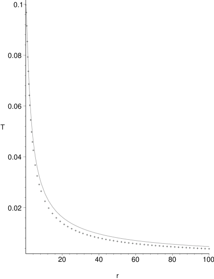
Figure 1: Graph of $T(r)$. The graph with the dotted line is that of $T_{1}$; the solid line is the graph of $T_{1}+\epsilon T_{2}$.

4 The RG Flow with a tachyon

We now consider the RG flow itself, rather than the fixed points. When the tachyon is zero, the beta functions were computed in [15, 4]. When there is a non-zero tachyon, the beta functions computed in [16] yield the flow equations (assuming the central charge term in the dilaton beta function is zero)

$$\dot{g}_{ij} = -\alpha^{\prime}(R_{ij}+2\phi_{|ij}-T_{,i}T_{,j});$$ (36)

$$\dot{\phi} = {\alpha^{\prime}\over 2}(\Delta\phi-2|\nabla\phi|^{2}-V(T)));$$ (37)

$$\dot{T} = \alpha^{\prime}(\Delta T-2\nabla\phi\cdot\nabla T-V^{\prime}(T)).$$ (38)

The dot refers to derivative with respect to the RG flow parameter (logarithm of scale).

An interesting feature of these flow equations seems to be that the dilaton cannot be decoupled from the metric and tachyon flow by a choice of gauge (as it can be when the tachyon is zero). Curiously, if the beta function of the tachyon were multiplied by an overall factor of ${1\over 2}$, then a decoupling of the dilaton would have been possible in the resulting flow equations.

We now look for special solutions to the flow equations. We are motivated by the conjecture that in certain situations, the RG flow can model on-shell time evolution (for an elaboration of when this applies, see [1]). By on-shell time evolution, we mean spacetime metrics obtained by solving the fixed point equations.

We are interested in whether there are RG flow solutions that are similar to the tachyon cosmologies discussed by Yang and Zweibach [3].

The tachyon cosmology of Yang and Zweibach is a solution of Eq.(1-3) with $c=0$ and a Lorentzian metric of the form

$$ds^{2}=-dt^{2}+a(t)\delta_{ij}dx^{i}dx^{j},$$ (39)

and with dilaton and tachyon fields dependent only on the time coordinate $t$. In [3], tachyon-induced rolling is studied. When the tachyon potential is of the form Eq.(23) (i.e, only leading order term), then tachyon-induced rolling implies that $da/dt=0$, so that the string frame metric does not evolve. For other potentials, it is possible to find solutions with $da/dt=0$.

We examine RG flow equations for two tachyon potentials studied in [3]. In an abuse of notation, in what follows, $t$ will be used to denote the RG flow parameter. This makes it easier to compare with the solutions in [3]; however, the RG flow parameter is not, in general, the same as the dynamical time of those solutions. Rather, we would like to explore, for two choices of potentials $V(T)$, if $t$ indeed behaves like the dynamical time. We look for solutions to RG flow with Riemannian metrics and the ansatz that the tachyon and the dilaton only depend on $t$ (RG flow parameter) with the metric of the form

$$ds^{2}=a(t)\delta_{ij}dx^{i}dx^{j}.$$ (40)

With this ansatz, it trivially follows that $a(t)$ is a constant; so the metric does not evolve for any choice of tachyon potential.

Now we assume a tachyon potential of the form Eq.(23) with just the lowest order term. We get the solutions

$$a(t) = a;$$

$$T(t) = T_{0}e^{\alpha^{\prime}m^{2}t};$$

$$\phi(t) = {T_{0}^{2}\over 8}e^{2\alpha^{\prime}m^{2}t}.$$ (41)

Here, $a$ is used to denote a constant. So, in agreement with Yang and Zweibach, the metric (if interpreted as a string frame metric) is constant, the tachyon induces rolling at $t=-\infty$ and the solutions themselves look very similar near $t=-\infty$ to the solutions in [3] for the corresponding potential, except that $m$ is now replaced by $m^{2}$. As $t\to\infty$, both the tachyon and dilaton diverge. If the above metric were indeed a string frame metric, the ‘Einstein frame metric’

$$g^{E}_{ij}:=e^{-2\phi(t)}g_{ij},$$ (42)

is constant (in $t$) and regular near $t=-\infty$. On the other hand, as $t\to+\infty$, the Einstein frame metric crunches to a point (conformal factor goes to zero).

This nice similarity to solutions of dynamical evolution does not hold for other choices of potentials. For $V(T)=-{1\over 2}~{}m^{2}\left(T^{2}-T^{4}/4\right)$, there are two branches of solutions to the RG flow equations. One branch corresponds to singular tachyonic initial condition, so we disregard it. For the other branch, we find that

$$a(t) = a;$$

$$T(t) = \sqrt{2}\frac{T_{0}e^{\alpha^{\prime}m^{2}t}}{\sqrt{1+T_{0}^{2}e^{2\alpha^{\prime}m^{2}t}}};$$

$$\phi(t) = \phi_{0}+\alpha^{\prime}{m^{2}\over 4}t-{1\over 8}\ln\left[\frac{T_{0}^{2}e^{2\alpha^{\prime}m^{2}t}}{1+T_{0}^{2}e^{2\alpha^{\prime}m^{2}t}}\right]-\frac{1}{8(1+T_{0}^{2}e^{2\alpha^{\prime}m^{2}t})}.$$ (43)

As we said earlier, the metric does not evolve. The behaviour of the tachyon and the dilaton for the above solution in various limits is as follows:

• Although the dilaton has a linear term, one finds on careful analysis that as $t\to-\infty$, the linear term cancels out with contributions coming from other terms. The integration constant $\phi_{0}$ can be chosen such that the dilaton goes to zero as $t\to-\infty$. In fact, it then goes to zero as $e^{2\alpha^{\prime}m^{2}t}$. In this limit, the tachyon goes to zero slower, as $e^{\alpha^{\prime}m^{2}t}$. Therefore the tachyon induces the rolling at $t=-\infty$.

• As $t\to\infty$, the dilaton grows linearly with $t$. The tachyon instead settles to the constant value $\sqrt{2}T_{0}$. Thus the corresponding ‘Einstein frame’ metric crunches in this limit to a point, due to the behaviour of the dilaton.

This solution (particularly the tachyon) behaves differently from Yang and Zwiebach’s dynamical solution for the potential we chose, except at early times when the tachyon induces the rolling. This is not in itself surprising. The phase space of solutions to the dynamical equations is bigger than that for the RG flow, and the similarity between the two seems to hold only for a particular time dependence of the tachyon and dilaton.

Acknowledgments
The authors wish to thank the Natural Sciences and Engineering Research Council of Canada for partial support. V.S would like to thank B. Sathiapalan for a discussion on the tachyon beta function and E. Woolgar for comments on the paper. We would also like to thank the referee for bringing [12] to our attention.

References

- [1] M Headrick, S Minwalla and T Takayanagi, Class Quant Grav 21 (2004) S1539 [hep-th/0405064] and references therein.
- [2] A Adams, X Liu, J McGreevy, A Saltman and E Silverstein, JHEP 0510 (2005) 033 [hep-th/0502021]; S Hirano, JHEP 0507 (2005) 017 [hep-th/0502199]; T Suyama, JHEP 0505 (2005) 065 [hep-th/0503073]; J McGreevy, E Silverstein, JHEP 0508 (2005) 090 [hep-th/0506130]; M Spradlin, T Takayanagi and A Volovich, JHEP 0511 (2005) 039 [hep-th/0509036]; K Narayan, JHEP 0603 (2006) 036 [hep-th/0510104]; DZ Freedman, M Headrick and A Lawrence, Phys Rev D73 (2006) 066015 [hep-th/0510126]; T Suyama, JHEP 0603 (2006) 095 [hep-th/0510174]; J-H She, [hep-th/0512299]; GT Horowitz and E Silverstein, Phys Rev D73 (2006) 064016 [hep-th/0601032]; E Papantonopoulos, I Pappa and V Zamarias, to appear in JHEP [hep-th/0601152]; E Silverstein [hep-th/0602230]; T Suyama [hep-th/0605032].
- [3] H Yang, B Zwiebach, JHEP 0508 (2005) 046 [arxiv: hep-th/0506076]; JHEP 0509 (2005) 054 [arxiv: hep-th/0506077].
- [4] CG Callan, D Friedan, EJ Martinec and MJ Perry, Nucl Phys B262 (1985) 593.
- [5] G Curci and G Paffuti, Nucl Phys B286 (1987) 399.
- [6] H Osborn, Ann Phys (NY) 200 (1990) 1.
- [7] E Witten, Phys Rev D44 (1991) 314.
- [8] G Mandal, AM Sengupta, SR Wadia, Mod Phys Lett A6 (1991) 1685.
- [9] T Oliynyk, V Suneeta, E Woolgar, Phys Lett B21739 (2005) [arxiv:hep-th/0410001].
- [10] J-P Bourguignon in Global differential geometry and global analysis, Lectures in Mathematics 838, ed D Ferus (Springer, Berlin, 1981).
- [11] N. Marcus and Y. Oz, Nucl Phys B407 (1993) 429.
- [12] A Peet, L Susskind and L Thorlacius, Phys Rev D48 (1993) 2415. See also G.A. Diamandis, B.C. Georgalas and E. Papantonopoulos, [arxiv: hep-th/9406028] and J.D. Hayward, [arxiv: hep-th/ 9502062] for some further work on this subject.
- [13] M. Abramowitz and I. A. Stegun, Handbook of Mathematical Functions, NY, Dover Publications, 1970.
- [14] R Dijkgraaf, H Verlinde, E Verlinde, Nucl Phys B371 (1992) 269.
- [15] G Ecker and J Honerkamp, Nucl Phys B35 (1971) 481; DH Friedan, Phys Rev Lett 45 (1980) 1057; ES Fradkin and AA Tseytlin, Phys Lett B158 (1985) 316.
- [16] SR Das and B Sathiapalan, Phys Rev Lett 56 (1986) 2664; R Brustein, D Nemeschansky and S Yankielowicz, Nucl Phys B301 (1988) 224; A Cooper, L Susskind, L Thorlacius, Nucl Phys B363 (1991) 132.