Orientifolds, hypercharge embeddings and the Standard Model

Abstract:

The embedding of the SM hypercharge into an orientifold gauge group is studied. Possible embeddings are classified, and a systematic construction of bottom-up configurations and top-down orientifold vacua is achieved, solving the tadpole conditions in the context of Gepner orientifolds. Some hypercharge embeddings are strongly preferred compared to others. Configurations with chiral antisymmetric tensors are suppressed. We find among others, genuine examples of supersymmetric SU(5), flipped SU(5), Pati-Salam and trinification vacua with no chiral exotics.

1 Introduction

During the past twenty years it has become clear that the information String Theory gives us about the Standard Model (SM) is extremely complex. It does not seem that String Theory, or some selection principle on top of it, will gives us a unique four-dimensional gauge theory that is identical to the Standard Model. On the other hand, there may be non-trivial restrictions on the kind of gauge theories that can emerge from String Theory, and it is not a priori obvious that the Standard Model satisfies those restrictions.

In this situation, there are several approaches one can follow. It would be a tremendous success if one could find a string vacuum that precisely matches all current experimental constraints. For many years it seemed plausible that those constraints would be restrictive enough to reduce the number of vacua to (at most) a single one. The hope was that, having found that vacuum, we would see all the remaining pieces of the puzzle fall into place, and we could start making falsifiable predictions for future experiments.

However, it now seems wishful thinking to believe that this will actually be true. Although reliable estimates cannot be made, naive guesses suggest that the number of vacua meeting all current experimental constraints may well be much larger than 1. Even in that situation, finding just one of those would be a huge success, at least as an existence proof. But making predictions based on such a vacuum is a rather delicate affair if one does not know the complete ensemble of vacua satisfying all current constraints. This does not mean that no further predictions can be made. There is no reason to expect the moment of discovery of the landscape of string theory, [1], [2] to coincide with the end of such successful theoretical predictions. But all successes of the past (such as the relation between $\alpha$ and $g-2$) can be understood in terms of the quantum field theory description of the Standard Model. There may be further successes of this kind, but what one would really hope to find is a genuine string prediction.

At present too little is known about the set of String Theory vacua to be able to say how far this programme can be pushed. One extreme might be that the problem is too (NP)hard for us to solve [3], and that we will have to be satisfied with having a certain degree of confidence that the Standard Model does indeed exist somewhere in the landscape, just as we are confident that the DNA molecule is a solution of QED, without being able to write it down explicitly. To accept such an outcome would require, at the very least, some kind of confirmation that String Theory is the correct theory of Quantum Gravity. The other extreme is that the potentially huge set of unfixed degrees of freedom do not actually exist for the Standard Model, or are confined to an irrelevant sub-sector, such as a barely observable (“hidden”) sector.

In either case it is clearly essential to expand our knowledge of the landscape of string vacua by all means at our disposal and to understand the possible realizations of vacua that have the SM as a low energy limit. There are two approaches to that end. The first is the top-down approach that constructs string vacua using CFT techniques and then checks whether their low energy limit compares favorably to the SM. This approach has been used extensively in heterotic model building, and more recently in orientifold model building.

The other approach is the bottom up approach that has been especially suited to the orientifold context, [4, 5]. This is because the back-reaction of a brane-configuration comes-in at the next order in the coupling constant expansion. It has slowly become clear that in searching for the SM-like vacua, a combination of the two approaches may be the most efficient one.

In this paper, we want to make some modest steps towards understanding the complexity of the landscape, and in particular the different possibilities for realizing SM-like vacua. In particular, it is known that there are several possible embeddings of the SM hypercharge into the orientifold gauge group [4, 6, 7]. Such embeddings affect crucial phenomenological properties of the vacua. It is therefore important to analyze such embeddings. For this, instead of focusing on a particular model we will try to broaden the scope as much as possible. In [11], [12] two of the authors presented a detailed investigation of a piece of the landscape that until then was barely accessible: orientifolds of Gepner models. The approach of these papers can be described as a mixture of a top-down and a bottom-up method. On the one hand, exact string solutions were looked for and found. But on the other hand, the kind of solutions that were searched were limited a priori by a choice of a “bottom up” realization of the Standard Model, constructed out of intersection sets of branes.

The scope of the RCFT method, even when restricted to Gepner models, seems to be considerably larger than that of the much more extensively studied orbifold models. Indeed, the first example of a supersymmetric spectrum that matches the standard model exactly (in the chiral sense) was found using an RCFT construction in [11]. This was an amazing eight years after the first steps towards realistic model building with orientifolds were taken [13], using orbifold methods. Since that pioneering paper, the orbifold/orientifold method has been explored extensively by many authors (see [14] and references therein) who succeeded in getting ever closer to the supersymmetric standard model spectrum, until that goal was finally reached in [15] for the $Z_{6}$ orbifold.

During the same period there has been relatively little work on Gepner orientifolds [16]-[21], and with relatively little success, the first paper finding a chiral spectrum being [19] in 2004. However, it is now clear that the lack of success was due to the fact that until recently only a limited number of partition functions and boundary states was accessible. A recent investigation [22] of $Z_{2}\times Z_{2}$ orbifolds has shown that the three family standard model spectrum is just beyond the limit of statistics in that case. By contrast, with Gepner models more than 200.000 standard model realizations were found in [12], despite the fact that the average success rate is actually lower (empirically, “one in a billion” for $Z_{2}\times Z_{2}$ orbifolds, and about $4\times 10^{-14}$ for Gepner models).

On the other hand, RCFT methods also have clear disadvantages in comparison to orbifold methods. In particular, they do not allow continuous variations of moduli, and are not suitable for discussions of flux compactifications and moduli stabilization, at least not without radically new ideas. But their larger scope makes them ideally suited for scanning a substantially larger part of the landscape than was possible up to now, provided one focuses only on issues related to spectroscopy. This is precisely our goal in this paper. Our main phenomenological input will be the chiral spectrum of the standard model. Our intention is to loosen considerably the bottom up assumptions made in [12], and investigate a large number of other ways of realizing the standard model with D-branes (or boundary states).

The kind of bottom up models considered in [12] were variations on the model first proposed in [6]. They are characterized by four stacks of branes with a Chan-Paton group $U(3)_{\bf a}\times U(2)_{\bf b}\times U(1)_{\bf c}\times U(1)_{\bf d}$, with the standard model generator $Y$ embedded as $Y=\frac{1}{6}Q_{\bf a}-\frac{1}{2}Q_{\bf b}-\frac{1}{2}Q_{\bf c}$. The variations include the possibility of choosing the second and third Chan-Paton factor real, and allowing the $B-L$ abelian vector boson to be either massive or massless in the exact string theory. These models have a perturbatively unbroken baryon and lepton number.

Many other brane realizations exist, and some of those have been discussed in the literature. To obtain the results of [12] a huge effort was required in terms of computer time. In principle, this project could be redone for anyone’s favorite bottom-up model. However, it seems preferable to try to remove the bias implied by a particular choice of model, and try to repeat the computation assuming as little as possible about the bottom-up realization.

In principle, the only feature we assume is the most robust part of what we presently know about the Standard Model: that there are three chiral families of quarks and leptons in the familiar representations of $SU(3)\times SU(2)\times U(1)$. In practice, we still have to make a few concessions. In particular, we will have to limit the number of participating branes and forbid non-chiral mirror pairs of arbitrary charge. This will be discussed in more detail in the next section.

The new features that we do allow include

• Anti-quarks realized as anti-symmetric tensors of $U(3)$

• Charged leptons and neutrinos realized as anti-symmetric tensors

• Non-standard embeddings of the $Y$-charge

• Embeddings of $Y$ in non-abelian groups

• Strong-Weak unification (e.g. $SU(5)$)

• Baryon-lepton unification (e.g. Pati-Salam models)

• Trinification

• Baryon and/or lepton number violation

• Family symmetries

We are not claiming that all of these features are desirable, but our strategy is to allow as many possibilities in an early stage, and leave the final selection to the last stage, so that it will not be necessary to restart the entire search procedure if new insights emerge.

Some of these options may address unsolved problems that occur for the standard realization [6] of the standard model. For example, the perturbatively unbroken lepton number of these models makes it hard to implement a see-saw like mechanism to give small masses to neutrinos. Coupling constant unification, if it is indeed a fundamental feature of nature and not a semi-coincidence, is not automatic in the standard realization, but it would be in $SU(5)$ models. This does not mean that the standard realization cannot accommodate the current experimental values of the couplings constants, but only that the fact that they presently appear to converge (with gaugino contributions taken into account) would be a mere coincidence. We have indeed found some really simple and elegant realizations of $SU(5)$ models, but unfortunately we did not find a credible mechanism for generating up-quark masses. We will comment on this and on the viability of some of the other options in section 7.

One of our goals is to analyze which model can be built from a bottom-up point of view, and how many of them can be realized as top-down models. By “bottom-up” we mean here a brane realization that produces the correct chiral standard model spectrum if the gauge group is reduced to $SU(3)\times SU(2)\times U(1)$ (without assuming a particular mechanism for that reduction). On the “top-down” side two types of concepts should be distinguished: standard model brane configurations and solutions to the tadpole conditions. The focus in this paper is on the former, i.e. choices of boundary labels a, b, c and d such that with an appropriate choice of the Chan-Paton gauge group and the appropriate embedding of $SU(3)\times SU(2)\times U(1)$ one obtains the standard model. Here we also require that the standard model $U(1)$ generator does not acquire mass due to bilinear axion couplings.

Given such a standard model configuration, there may still be uncancelled tadpoles in RR closed string one-point functions on the disk and the crosscap. Within this context, the only way to cancel them is to add additional hidden matter, except in a few cases where they already cancel among the standard model branes. To see if this can happen is an extremely time-consuming, and ultimately unsolvable problem. Furthermore for any given brane configuration there may be many ways of cancelling the tadpoles. In the continuum theory, background fluxes, not considered here, contribute to the tadpoles. But perhaps more importantly, the set of boundary states we consider here is limited by the choice of rational CFT. We consider the complete set of boundaries allowed by the RCFT, i.e. all boundaries that respect its chiral algebra. But that chiral algebra is larger than the $N=2$ world-sheet algebra required to describe a geometric Calabi-Yau compactification. Since we get the $c=9$ chiral algebra as a tensor product of minimal $N=2$ algebras, the chiral algebra also contains all differences of the $N=2$ algebras of the factors. If we would reduce the chiral algebra, additional boundary states are allowed, and could contribute to tadpole cancellation. Of course this also allows additional ways of constructing standard model configurations, but we cannot make regarding a complete classification there anyway.

It is essentially impossible to conclude, with RCFT techniques alone, that the tadpoles of a certain standard model configuration cannot be cancelled. Positive results, on the other hand, imply that one has a valid supersymmetric string vacuum. We see tadpole cancellation therefore mainly as an existence proof of a given string vacuum. Once that proof has been given, we do not continue searching for additional tadpole solutions for the same chiral configuration. This gives an enormous cut-off in computer time. One should keep in mind that for the most frequent chiral model considered in [12], we found a total of 16 million tadpole solutions (about 110000 of them distinct). We now keep only one of those solutions. This also implies that we cannot provide meaningful statistical results regarding tadpole solutions, but only regarding brane configurations.

We summarize briefly our results:

• We develop a detailed classification of allowed embeddings of the SM hypercharge inside the orientifold gauge group. To do this, we classify brane stacks according to how they contribute to the hypercharge. The hypercharge embedding is then characterized by a real variable $x$ which is quantized in half-integral units in genuine non-orientable vacua.

• We produce 19345 chirally distinct top-down SM spectra (before tadpole cancellation) and 1900 chirally distinct models solving the tadpole conditions and realizing the different embeddings.

• We find that the $x={1\over 2}$ hypercharge embedding dominates by far all other choices. The Madrid embedding [6] belongs to this class.

• The presence of chiral symmetric and antisymmetric tensors is highly suppressed. For some hypercharge embeddings, such tensors are crucial for anomaly cancellation and they may produce anti-quarks and other weak singlets. This implies the associated suppression of such embeddings.

• We produce the first examples of supersymmetric SU(5) and flipped SU(5) orientifold vacua, with the correct chiral spectrum (no extra gauge groups and no exotic $G_{CP}$ chiral states). However, as we argue, all such orientifold models, as well as models with quarks in the antisymmetric representation have a serious phenomenological problem associated with masses.

• We find some minimal supersymmetric Pati-Salam and trinification vacua.

• We have examples of spectra (but no tadpole solutions yet) with extended (N=4 or N=8) supersymmetry in the bulk and N=1 supersymmetry on the branes.

• We have found SM spectra solving the tadpole conditions on a relative of the quintic CY.

This paper is organized in follows. In the next section, we define precisely what our criteria for standard model realizations are. In section 3, we work out the consequences of these criteria from the bottom-up point of view. We classify these models in terms of a parameter $x$ which determines the embedding of $Y$ in the a and b stacks. We first identify a class of models for which $x$ is undetermined by the quark and lepton charges. In all other models $x$ is half-integer, with $x=0$ corresponding to $SU(5)$-type models [7] as well as models A,A’in [4, 23], $x=\frac{1}{2}$ to Madrid-type configurations, [6], and $x=1$ in models B,B’ in [4, 23]. We present some explicit realizations of each type of model, and also identify possible lepton number symmetries and Higgs boson realizations. In section 5 we present the results of a search for orientifolds of Gepner models. We limit ourselves to simple current modular invariant partition functions (MIPFs) with at most 1750 boundaries. In section 6 we present a small sample of the tadpole solutions that we have found, providing concrete example of a variety of types of models. In section 7 we discuss the viability of various features of models we found, focusing mainly on masses. Finally in section 8 we examine correlations between the topology of the CY manifold, and the features of the SM realization.

In appendix A we explain in detail the search algorithm for these configurations in RCFT orientifolds. In appendix B, we examine the correlation between gauge coupling constants, and the allowed values for the string scale for different hypercharge embeddings.

2 What we are looking for

Our goal is to search for the most general embedding of the standard model in the Chan-Paton gauge group of Gepner Orientifolds.

We first introduce some notation. We denote the full Chan-Paton group as $G_{\rm CP}$. This is the group obtained directly from the multiplicities of the branes, without taking into account masses generated by two-point axion-gauge boson couplings. We require that the standard model gauge group, $G_{\rm SM}=SU(3)\times SU(2)\times U(1)_{Y}$ is a subgroup of $G_{\rm CP}$. Furthermore we require that the generator of $U(1)_{Y}$ does not get a mass from axion-gauge boson couplings.

The main condition we impose on the spectrum is the presence of three families of quarks and leptons, and the absence of chiral exotics. Since chirality can be defined with respect to various groups, and the term “exotics” is used in different senses in the literature, we will define this more precisely. Group-theoretically, the standard-model-like spectra we allow are described as follows. Denote the full set of massless representations of $G_{\rm CP}$ as $R_{\rm CP}$. The subset of these representations that is chiral with respect to $G_{\rm CP}$ is denoted $R^{\rm chir}_{CP}$. The reduction of these representations to the the group $G_{\rm SM}$ are denoted as $R_{\rm SM}$ and $R^{\rm chir}_{\rm SM}$ respectively. By “reduction” we mean here only that we decompose representations in terms of representations of a subgroup. No assumptions are made at this point regarding dynamical mechanisms (like the Brout-Englert-Higgs mechanism) to achieve such a reduction. Consider now the subset of either $R_{\rm SM}$ or $R^{\rm chir}_{\rm SM}$ that is chiral with respect to $G_{\rm SM}$. The result is required to be precisely the following set of left-handed fermions (all fermions will be in left-handed form in this paper)

$$3\times[(3,2,\frac{1}{6})+(3^{*},1,-\frac{2}{3})+(3^{*},1,\frac{1}{3})+(1,2,-\frac{1}{2})+(1,1,1)]$$ (2.1)

Any other particles must be non-chiral with respect to $G_{\rm SM}$. This may include left-handed anti-neutrinos in the representation $(1,0,0)$ and MSSM Higgs pairs, $(1,2,\frac{1}{2})+(1,2,-\frac{1}{2})$. Anything else will be called exotic.

The foregoing describes the most general configuration one could reasonably call an embedding of the standard model without chiral exotics, but we will have to impose a few additional constraints to make a search feasible. First of all we require that the standard model groups $SU(3)$ and $SU(2)$ come each from a single stack of branes, denoted a and b respectively. This forbids diagonal embeddings of these groups in more than one CP factor. In general by a stack we mean a single label for a real (orthogonal or symplectic) boundary, or a pair of conjugate labels for complex, unitary branes. The CP factor yielding $SU(3)$ must be $U(3)$, whereas the weak gauge symmetry $SU(2)$ can come from either $U(2)$ or $Sp(2)$. The group $O(3)$ is not allowed, because one cannot get spinor representations of orthogonal groups in perturbative open string constructions.

The hypercharge generator $Y$ is a linear combination of the unitary phase factors of $U(3)$, $U(2)$ (if available) and any other generator of one of the other factors in $G_{\rm CP}$. All representations $(3,2)$ must necessarily come from bi-fundamentals of the a and b stacks, but not all anti-quarks can come from those stacks. Although there can be anti-quarks due to chiral anti-symmetric tensors of $SU(3)$, they all have the same hypercharge. Hence there must be at least one other stack of branes, labeled c.

In principle there could be any number of additional stacks of branes, but for purely practical reasons we allow at most one more stack (labeled d) to contribute to the standard model representation (2.1). Additional branes may be present, and may be required for tadpole cancellation. They will be referred to as the “hidden sector”. If stack d does not contribute to (2.1) at all we regard it as part of the hidden sector. The standard model branes a, b,c (and d, if present) will be called the “observable sector”. Note that left-handed anti-neutrinos are not listed in (2.1). We do not impose an a priori constraint on the number of left-handed anti-neutrinos, although in some cases a certain number of such states is required by anomaly cancellation in $G_{\rm CP}$. They may in fact come from the hidden sector or the observable sector, or even from strings stretching between the two sectors.

Our next condition concerns the precise definition of the standard model generator $Y$. We allow it to be embedded in the most general way possible in the Chan-Paton factors of brane c and d (in addition to the unitary phases of a and b). In principle it could also have components in the hidden sector without affecting any of the foregoing, as long as all particles charged under those components of $Y$ are massive or at least non-chiral. One could even try to use this as a mechanism to cancel bilinear axion coupling of $Y$, which would give the $Y$-boson a mass. We will not consider that possibility here. This is equivalent to a restriction to standard model realizations with at most four participating branes, except for one intriguing possibility: a three brane realization with a fourth brane added purely to fix the axion couplings of $Y$, without contributing to quarks or leptons. This possibility was not included in our search. It should be mentioned however, that a qualitatively similar situation does indeed arise. There are orientifold vacua where there is a U(1) arising from the SM stack of branes , under which all SM particles are neutral. In this case there is a continuous family of possible hypercharge embeddings. In some cases, the masslessness condition breaks the degeneracy. This provides a string realization of the field theory models in [25]. In other cases, even the masslessness condition does not lift the degeneracy.

The general form of $Y$ is

$$Y=\sum_{\alpha}t_{\alpha}Q_{\alpha}+W_{\bf c}+W_{\bf d}\ ,$$ (2.2)

where $\alpha$ runs over the values a,b,c,d, $Q_{\alpha}$ is the brane charge of brane $\alpha$ ($+1$ for a complex brane, $-1$ for its conjugate, and 0 for a real brane), and $W_{\bf c}$ and $W_{\bf d}$ are generators from the non-abelian part of the Chan-Paton group. Therefore $W_{\bf c}$ and $W_{\bf d}$ are traceless. Such contributions to $Y$ occur for example in Pati-Salam and trinification models, and therefore we want to allow this possibility.

There is one more condition we impose for practical reasons, namely that $R^{\rm chir}_{CP}$ may only yield representations of standard model particles or their mirrors. The main purpose of this condition (as we will see in more detail below) is to prevent an unlimited proliferation of $G_{\rm CP}$-chiral, but $G_{\rm SM}$ non-chiral representations such as $(1,1,q)+(1,1,-q)$, with $q$ arbitrary. In addition, this condition also forbids triplets of $SU(2)_{\rm weak}$, which can be chiral with respect to $U(2)_{\bf b}$.

One may distinguish three types of matter in these models: OO, OH and HH, where the two letters indicate if the endpoints of the open string are in the observable or hidden sector. All conditions on OO matter were already formulated above. The “no chiral exotics” constraint formulated above allows HH matter to be chiral with respect to $G_{\rm CP}$. For OH matter we impose a somewhat stronger constraint, namely that there cannot be any bi-fundamentals between the standard model and the hidden sector that are chiral with respect to $G_{\rm CP}$. This is a stronger condition because the “no chiral exotics” constraint allows SM-Hidden sector bi-fundamentals as long as they are non-chiral with respect to $G_{\rm SM}$. For example a mirror quark pair $(3,V)+(3^{*},V)$, where $V$ is a vector in a hidden sector $U(N)$ group, could be allowed under the more general rules. The resulting $U(N)$ anomalies can be cancelled in various ways.

We will allow the brane stacks ${\bf a}$, ${\bf b}$, ${\bf c}$, ${\bf d}$ to have identical labels, with the exception of c and d (if they are identical, we might as well regard them as a single brane stack with a larger CP multiplicity). By allowing identical labels we are able to obtain examples of unified models, such as (flipped) SU(5) or Pati-Salam like models. In the case of identical labels, we count them as follows: the QCD and weak group count as one stack each, and the branes that remain after removing the QCD and weak groups count as additional stacks, such that the total does not exceed four. For example, we can get $U(5)$ models with at most two additional CP-factors (plus any number of hidden sector branes).

We conclude this section with a summary of the kind of “exotics” (plus singlets and Higgs candidates) that may occur in generic models, indicating which kind we do and do not allow. We split $G_{\rm CP}$ into an observable and a hidden part as $G_{\rm O}\times G_{\rm H}$. In all cases we combine representations into non-chiral sets (usually, but not always pairs) if possible. We can distinguish the following possibilities

1. Matter of type OO

   1. Non-chiral with respect to $G_{\rm CP}$. This may include symmetric and anti-symmetric tensors or adjoints of $SU(3)$ or of SU(2), mirror pairs of quarks and leptons, as well as bi-fundamentals with unusual and in a few cases even irrational charges. All particles in this class are allowed by our conditions.

   2. Chiral with respect to $G_{\rm CP}$, non-chiral with respect to $G_{SM}$. Examples are symmetric tensors of $U(2)_{\rm weak}$, mirror pairs of quark and lepton doublets that are chiral with respect to $U(2)_{\rm weak}$, mirror pairs where one member of the pair is a rank-2 tensor and the other member a bi-fundamental. We do allow such particles, except the symmetric $U(2)_{\rm weak}$ tensors, and non-chiral pairs of quarks and leptons with non-standard charges.

   3. Chiral with respect to $G_{\rm CP}$, chiral with respect to $G_{\rm SM}$, non-chiral with respect to $\rm{QED}\times\rm{QCD}$. An example of such exotics would be a fourth family. Exotics of this type are not allowed by our conditions.

   4. Chiral with respect to $G_{\rm CP}$, chiral with respect to $G_{\rm SM}$, and chiral with respect to $\rm{QED}\times\rm{QCD}$. Clearly this is not acceptable.

   A mass term for exotics of type 1a is allowed by the full gauge symmetry, and hence it is possible that such a term is generated by shifting the moduli of the model. It is an interesting question whether the appearance of such exotics is a special feature of RCFT, or if they persist outside the rational points. It should be possible to get some insight in this question by analyzing the coupling of these particles to the moduli, but this is beyond the scope of this paper. Exotics of type 1b may get a mass without invoking the standard model Higgs mechanism, and hence may become more massive than standard quarks and leptons. However, this will always require some additional dynamical mechanism beyond perturbative string theory. Exotics of type 1c require the standard model Higgs mechanism to get a mass. This may not be sufficient, since the Higgs couplings themselves may be forbidden by string symmetries, in which case additional mechanisms must be invoked. In any case it would be hard to argue that such particles would be considerably more massive than known quarks and leptons.

2. Matter of type HH. These are standard model singlets. No constraints are imposed on this kind of matter. One may distinguish two kinds.

   1. Non-chiral with respect to $G_{\rm CP}$. These particles may get a mass from continuous deformations of the model, as above.

   2. Chiral with respect to $G_{\rm CP}$, non-chiral with respect to $G_{\rm H}$. These particles may get a mass from hidden sector dynamics.

3. Matter of type OH. In many cases particles in this class have half-integer charge. This occurs if the electromagnetic charge gets a contribution $\frac{1}{2}$ from each observable brane, which turns out to be the most frequently occurring kind of model. There are many possibilities for the chiralities, which we list here for completeness. We use a notation $(\chi_{G_{\rm CP}},\chi_{G_{\rm H}},\chi_{G_{\rm O}},\chi_{G_{\rm SM}},\chi_{\rm{QED}\times\rm{QCD}})$, where each $\chi$ indicates chirality, and can be $Y$ (yes) or $N$ (no).

   1. (N,N,N,N,N).

   2. (Y,N,N,N,N).

   3. (Y,Y,N,N,N).

   4. (Y,N,Y,N,N).

   5. (Y,N,Y,Y,N).

   6. (Y,N,Y,Y,Y).

   7. (Y,Y,Y,N,N).

   8. (Y,Y,Y,Y,N).

   9. (Y,Y,Y,Y,Y).

   An example of type 3b, chiral with respect to the full Chan-Paton group, but not with respect to any of its subgroups, is $(3,0,V)+(3^{*},0,V)+3\times(1,1,V^{*})+3\times(1,-1,V^{*})$ in $U(3)\times U(1)\times U(N)$, with the first two factors from $G_{\rm O}$ and the last from $G_{\rm H}$. Of all these possibilities, only 3a is allowed by our criteria. Types 3b, 3c and 3g might be tolerated on more general grounds, and types 3f and 3i are clearly unacceptable.

3 Classification of bottom-up embeddings

Here we will discuss the possible values of the coefficients $t_{\alpha}$ that occur in the brane decomposition of $Y$. We will use the following expression for $Y$:

$$Y=\sum_{\alpha}x_{\alpha}Q_{\alpha}\ ,$$ (3.3)

where $Q_{\alpha}$ is the $U(1)$ charge of brane $\alpha$. In contrast to (2.2) the sum is here not a priori restricted to a definite number of branes. In our search we will allow also the possibility that diagonal Lie algebra generators $W$ of $SO(N)$, $Sp(2N)$ or $SU(N)$ groups contribute to $Y$, but this can always be taken into account by splitting those groups into $U(m)$ factors according to the $W$ eigenvalues $e_{i}$. For example, if there are two distinct eigenvalues we get for symplectic groups $Sp(2N)$ a contribution $W_{\alpha}={\rm diag}(N\times(e),N\times(-e))$, which can be accommodated by splitting $Sp(2N)$ into conjugate brane stacks with a CP group $U(N)$ and a contribution $eQ_{\alpha}$. Geometrically, this means that the $2N$ symplectic branes are moved off the orientifold plane. The same reasoning applies to $O(2N)$ branes. If there are $O(2N+1)$ stacks, the assumption of at most two distinct eigenvalues only allows the traceless generator $W=0$ in (2.2), and hence such branes cannot contribute to $Y$ at all. Finally, $U(N)$ branes can contribute $t_{\alpha}Q_{\alpha}+{\rm diag}(n_{1}\times e_{1},n_{2}\times e_{2})$, with $n_{1}+n_{2}=N$, $n_{1}e_{1}+n_{2}e_{2}=0$. This can be regarded as two stacks $U(n_{1})\times U(n_{2})$ contributing $(t_{\alpha}+e_{1})Q_{\alpha_{1}}+(t_{\alpha}+e_{2})Q_{\alpha_{2}}$, so that $x_{\alpha_{1}}=t_{\alpha}+e_{1}$ and $x_{\alpha_{2}}=t_{\alpha}+e_{2}$ Therefore formula 3.3 covers all cases.

The brane configurations we consider here are subject to two constraints: the spectrum must match that of the standard model in the chiral sense, with chirality defined with respect to $SU(3)\times SU(2)\times U(1)$. Furthermore all cubic anomalies in each factor of the full Chan-Paton group must cancel. This must be true because we want to be able to cancel tadpoles, and tadpole cancellation imposes cubic anomaly cancellation (mixed anomalies are cancelled by the generalized Green-Schwarz mechanism). The tadpoles are usually cancelled by adding hidden sectors, which adds new massless states to the spectrum. We do not allow these to be chiral with respect to $SU(3)\times SU(2)\times U(1)$, and hence they cannot alter the cubic anomalies. The cubic anomaly cancellation conditions that are derived from tadpole cancellation are the usual ones for the non-abelian subgroups of $U(N)$, $N>2$. Vectors contribute 1, symmetric tensors $N+4$ and anti-symmetric tensors $N-4$, and conjugates contribute with opposite signs. But the same condition emerges even if $N=1$ and $N=2$. This means that for example a combination of three vectors and an anti-symmetric tensor is allowed in a $U(1)$ factor. This is counter-intuitive, because the anti-symmetric tensor does not even contribute massless states, so that one is left with just three chiral massless particles, all with charge 1. The origin of the paradox is that it is incorrect to call this condition “anomaly cancellation” if $N=1$ and $N=2$ and if chiral tensors are present. It is simply a consequence of tadpole cancellation; the anomaly introduced by the three charge 1 particles is factorizable, and cancelled by the Green-Schwarz mechanism.

One might entertain the thought that this peculiar $U(1)$ cancellation might have something to do with the fact that we have three families of standard model particles. For example, one could assign the same $U(1)$ charge to all quarks or leptons of a certain type, and then cancel this anomaly with anti-symmetric tensors. This would require this particle type to appear with a multiplicity divisible by three. Because the $U(1)$ is anomalous, it would acquire a mass via the Green-Schwarz term. However, although configurations of this kind can indeed be constructed, they are complicated and unlikely to occur. We did indeed find examples of $U(1)$ anomaly cancellations due to anti-symmetric tensors, but usually with a more complicated family structure that does not admit such an interpretation.

3.1 Orientable configurations

Let us now return to our goal of determining the possibilities for $Y$. We begin by demonstrating that in principle all real values of the leading coefficient $x_{\bf a}$ are allowed. Using the quark doublet charges we may write $Y$ as follows

$$Y=(x-\frac{1}{3})Q_{\bf a}+(x-\frac{1}{2})Q_{\bf b}+{\rm rest}$$ (3.4)

Here we assume (without loss of generality) that the quark doublets all come from bi-fundamentals $(V,V^{*})$ stretching between the QCD and the weak brane. The second entry could also be a $V$, but then we can conjugate $U(2)$ to obtain $(V,V^{*})$. A mixture of $V$ and $V^{*}$ is however not allowed if we want $x$ to take all real values; neither is a chiral anti-symmetric tensor in either $U(3)$ or $U(2)$, or the option of using $Sp(2)$ instead of $U(2)$. Here and in the following all representations are in terms of left-handed spinors.

Now we need lepton doublets. They can only be bi-fundamentals ending on the $U(2)$. The other end must be on a brane that contributes to $Y$ in such a way that the total charge is either $-\frac{1}{2}$ or $\frac{1}{2}$. The latter value is considered because in addition to lepton doublets, we also allow mirrors, or MSSM Higgs pairs. Again we will write these bi-fundamentals exclusively as $(V,V^{*})$ (the first entry corresponds to $U(2)$). Mixtures of $(V,V)$ and $(V,V^{*})$ between the same branes would fix $x$, and if there are no mixtures we can convert all bi-fundamentals to the form $(V,V^{*})$. The multiplicities of these bi-fundamentals may be negative, in which case we interpret them as $(V^{*},V)$.

Since we only allow $SU(2)$ doublets with charges $\pm\frac{1}{2}$, the possibilities for the charge coefficients of the new branes are $x$ or $x-1$. We refer to branes with these charges as “type C” and “type D” respectively (the QCD and weak branes are defined to be of type A and B respectively. We use small letters a, b, c, d, e,$\ldots$ to label different stacks, and capitals A,B,C,$\ldots$ to label their types, with respect to the hypercharge embedding. Branes a and b are always of type A and B, but there is no one-to-one correspondence for the other branes). Note that these types C and D become equivalent (up to conjugation) if and only if $x=\frac{1}{2}$. We are not requiring that the type C or D branes are identical for all leptons or Higgs, or each other’s conjugate, even if their charges would allow that.

Let $n_{1}$ be the net number of chiral states between brane b and all of the C-type branes, and $n_{2}$ the same for type D. To be precise:

$$n_{1}=\sum_{i}\left[(N(V,V^{*})_{{\bf b}C_{i}}-N(V^{*},V)_{{\bf b}C_{i}})\right]\ ,$$ (3.5)

where $N$ is the absolute number of massless states with given properties. We now impose anomaly cancellation in $U(2)$ (for three families)

$$-9+n_{1}+n_{2}=0\ ,$$ (3.6)

because no chiral tensors are allowed for generic $x$. We also impose the requirement of having three chiral lepton doublets

$$n_{1}-n_{2}=3$$ (3.7)

which can be solved to yield $n_{1}=6$ and $n_{2}=3$. Note that the anomaly conditions for the Chan-Paton factors at the other end can aways be satisfied for some of the solutions. This is because the solution allows all multiplicities of $N(V,V^{*})$ as well as $N(V^{*},V)$ to be multiples of three. If we make three open strings end on the same $U(1)$ brane, the corresponding $U(1)$ anomalies can always be cancelled by anti-symmetric tensors.

Next we need anti-quarks. Since for general $x$ anti-symmetric $U(3)$ tensors are not allowed, they must be bi-fundamentals between the $U(3)$ stack and other branes. If we introduce new branes for the anti-quark strings to end on, we can always arrange the configuration so that the anti-quarks are of the form $(V^{*},V)$. Then we need a brane of type C for down anti-quarks and a brane of type D for up anti-quarks. One may also use one of the already present branes of type C and D for this purpose, provided that only combinations $(V,V^{*})$ or $(V^{*},V)$ are used. Anything else implies a condition on $x$. Even if one uses distinct branes for all particle types, there are many ways to cancel the $U(1)$ anomalies using anti-symmetric tensors.

Finally we need charged lepton singlets and their mirrors. They can occur in four different ways for generic $x$:

1. With both ends on an existing brane of types C and D.

2. With one end on a previous C or D brane and one end on a new one. This would require new branes with various possible charges. In particular, it allows the following new charges: $x+1$, $x-2$ and their conjugates. We refer to these as types E and F. For $x=\frac{1}{2}$ these are each other’s conjugates, and for $x=\frac{3}{2},1,0$ and $-\frac{1}{2}$ some of the types C,D,E and F are equivalent.

3. With both ends on the same, new brane. This requires a new brane with $t_{\alpha}=\pm\frac{1}{2}$. We call this type G, unless it coincides with a previous type.

4. With both ends on two distinct new branes. This would in principle allow two new branes with contributions $y$ and $1-y$ to $Y$. Such branes (if they do not coincide with any previous type) will be called type H.

There are even more possibilities if one allows arbitrary numbers of additional branes for charged leptons. For example, one can connect new branes to types E and F with charge contributions $x-2$ or $x+3$, connect new branes to types G and H or add more branes of type H. By allowing mirror leptons one can build arbitrarily long chains of branes in this manner. However, this is too baroque to consider seriously, and can in any case not be realized with at most four branes, a restriction we will ultimately impose. Already the fourth option is then impossible.

Options three and four split the standard model into two chirally disconnected sectors (i.e. there are no chiral strings connecting the two). This implies that the $Y$ anomaly does not cancel in each sector separately, and hence the two components of the would-be $Y$-boson must have Green-Schwarz couplings to axions that give it a mass. In principle these contributions could cancel for $Y$, but that seems improbable, and hence reduces the statistical likelihood of this sort of configuration in a search. Furthermore lepton Yukawa couplings are perturbatively forbidden in such models.

The same four options exist for left-handed anti-neutrinos, but we do not impose any requirements on our construction with regard to their multiplicity. If they come from strings not attached to any of the previous branes, we regard them as part of the hidden sector. Furthermore, we do not allow $Y$ to have contributions from branes that do not couple to charged quarks and leptons. Otherwise one could extend $Y$ by arbitrarily large linear combinations that only contribute non-chiral states. This implies that we regard a brane configuration as complete (prior to tadpole cancellation) if all charged quark and leptons exist chirally, and if all cubic $U(N)$ anomalies cancel. This configuration may already contain a few candidate right-handed neutrinos, and additional ones may appear, after tadpole cancellation, from hidden sector states, or strings between the standard model and the hidden sector.

Clearly this still leaves a huge number of possibilities to realize this kind of configuration, but there is an obvious maximally economical choice, namely identifying all branes of equal charge with each other, and the brane with opposite charge with its conjugate. This then results in a $U(3)\times U(2)\times U(1)\times U(1)$ model with the following chiral spectrum

$$\noindent 3 \times (V,V^{*},0,0)$$

$$3 \times (V^{*},0,V,0)$$

$$3 \times (V^{*},0,0,V)$$

$$6 \times (0,V,V^{*},0)$$

$$3 \times (0,V,0,V^{*})$$

$$3 \times (0,0,V,V^{*})$$

Although we anticipated the possible need for anti-symmetric tensors, it turns out that they are not needed at all in this particular configuration. All anomalies are already cancelled. This is a consequence of standard model anomaly cancellation. The formula for $Y$ is

$$Y=(x-\frac{1}{3})Q_{\bf a}+(x-\frac{1}{2})Q_{\bf b}+xQ_{\bf c}+(x-1)Q_{\bf d}$$ (3.8)

This model has the feature that it can be realized entirely in terms of oriented strings, which of course implies that $x$ is not fixed. The converse is not true because one can allow $U(1)$ anti-symmetric tensors; they do not yield massless particles and hence give no restriction on $x$. By construction, this is the minimal realization of the standard model in terms of oriented strings. Oriented configurations (although more complicated than the one shown above) were considered earlier in [26][5] in the context of type-II theories.

One can generalize these orientable models further by allowing stack c and/or d to consist of several type C and D branes. The most general configuration can be denoted as $U(3)\times U(2)\times U(p_{1}+q_{1})\times U(p_{2}+q_{2})$, where $p_{1}$ is the number of type C branes on stack c, etc. To achieve this split we allow non-trivial generators $W_{\bf c}$ and $W_{\bf d}$ in the definition of $Y$. This gives an infinite set of solutions, all with at least three Higgs pairs (this follows from $U(2)$ anomaly cancellation). All these models have in fact precisely the same structure as the basic four-stack model above, except for an additional possibility that occurs if type C or D branes are in different positions (i.e. have different boundary labels). If in total three open strings are needed ending on brane C to get three anti-quarks, then if there are several type C branes the total number of such strings must be three. However, each multiplicity can be positive and negative, and hence cancellations are possible, that show up in the spectrum as additional mirrors on top of the basic configuration.

One of these cases corresponds to the “trinification” model [27, 28]. One starts with a gauge group $SU(3)_{\rm color}\times SU(3)_{L}\times SU(3)_{R}$ and matter in three copies of the representation $(V,V^{*},0)+(V^{*},0,V)+(0,V,V^{*})$. This configuration fits into our construction by starting with four stacks (a, b, c, d) with a CP group $U(3)\times U(2)\times U(1)\times U(3)$, and $Y=-\frac{1}{6}Q_{\bf b}+\frac{1}{3}Q_{\bf c}+W_{\bf d}$, where $W_{\bf d}$ is the $SU(3)_{\bf d}$ generator ${\rm diag}(\frac{1}{3},\frac{1}{3},-\frac{2}{3})$. The spectrum is three times $(V,V^{*},0,0)+(V,0,V^{*},0)+(V^{*},0,0,V)+(0,V,0,V^{*})+(0,0,V,V^{*})$. The trinification model is obtained by putting stacks b and c on top of each other. In terms of the foregoing discussion, this model has $x=\frac{1}{3}$, and three branes of type C (one from stack c and two from stack d) plus one brane of type D (from stack d). The value $x=\frac{1}{3}$ can easily be understood as follows: in a standard trinification model $Y$ is embedded entirely in $SU(3)$ factors, and cannot have components in the brane charges. Therefore in particular it cannot have any component in $U(3)_{\bf a}$.

The foregoing orientable standard model configurations can be realized in principle in non-orientable string theories. In these realizations the value of $x$ is often fixed by the requirement that $Y$ does not get a mass due to bilinear couplings with axions. Sometimes this yields rather bizarre looking solutions. For example, in our set of solutions there is one with $t_{a}=\frac{1}{33}$. There are also cases where $Y$ remains massless for any value of $x$.

3.2 Charge Quantization

There are further constraints on $x$ if one considers unoriented models. First of all, for generic values of $x$ the non-chiral part of the string spectrum contains states of fractional or even irrational charge, from $(V,V)$ bi-fundamentals or from rank-2 tensors. Since such states are always non-chiral, they may be massive, or become massive under perturbations of the model. They would however be stable and are not confined by additional gauge interactions, because they live entirely within the standard model sector. Therefore, although this possibility cannot be completely ruled out, it certainly seems preferable to avoid it.

The foregoing discussion is quite general, and can be used to analyse charge quantization for non-standard-model states in any brane realization of the standard model. The dependence on $Q_{\bf a}$ and $Q_{\bf b}$ in (3.8) is the most general one possible, up to an irrelevant sign choice. The complete string spectrum contains states with charges of all sums and differences of the components of $Y$, as well as all values multiplied by 2. It is easy to see that just from branes a and b, we get the charge quantization condition

$$x=0\hbox{~{}mod~{}}\frac{1}{2}\ ,$$ (3.9)

if we require that all massive open string states from bi-fundamentals and rank two tensors between standard model branes a and b to have integer charges (taking into account QCD confinement). Clearly this condition also implies charge integrality if branes of types C,D,E and F are present. Only if charged leptons come from a chirally decoupled sector (the third or fourth case listed earlier) further conditions may be needed.

A second type of fractional charges that may occur are those coming from strings with a single end on a standard model brane, and the other end on a hidden sector brane. Even if these states are non-chiral, they certainly exist as massive excitations. In principle, such charges could be confined by hidden sector gauge groups, but to avoid them altogether, the following condition must hold

$$x=0\hbox{~{}mod~{}}1\ .$$ (3.10)

Also this condition can be derived from just the a and b branes. If it is satisfied, branes of types C, D, E and F satisfy the hidden sector charge quantization condition, but types G and H do not, in general.

Note that the first charge quantization condition (absence of fractional charge within the standard model sector) is automatically satisfied in oriented strings for any $x$, because the strings that might violate it simply do not exist in oriented string theories. However, quantization conditions do arise if one wishes to include hidden branes. These should not contribute to $Y$. This imposes the second charge quantization condition, $x=0\hbox{~{}mod~{}1}$, for oriented strings.

3.3 Non-orientable configurations

The foregoing restrictions were necessary if one wishes to avoid non-chiral fractionally charged matter. More severe restrictions apply if some of the quarks and leptons themselves come from states that break the orientability of the open string theory.

Note first of all that in most cases both type C and type D branes are needed, in order to get up and down anti-quarks. The only way out is to get either all down anti-quarks or all up anti-quarks from anti-symmetric $U(3)$ tensors. The former possibility requires $x=\frac{1}{2}$, and then types C and D are the same. This possibility is realized in flipped $SU(5)$ models, of which we will give examples later. The second option leads to $x=0$. Then no type D brane is needed for the quarks, and type C branes do not contribute to $Y$. This possibility finds a natural realization in $SU(5)$ GUT models. For all other values of $x$ at least one type C and one type D brane is needed in addition to branes a and b.

Consider now the possibility that a chiral state (a quark or lepton, or a mirror) breaks the orientability of the configuration. Obviously this sort of analysis applies to each chirally decoupled subsector separately (connected components of quiver diagrams), and we will only consider the component connected to the a and b branes.

The possibilities for such a chiral state, and the resulting restrictions on $x$ are as follows

• Chiral anti-symmetric tensors on brane a; $x=0$ or $\frac{1}{2}$

• Chiral anti-symmetric tensors on brane b; $x=0$, $\frac{1}{2}$ or $1$

• $(V,V)$ between on branes a and b; $x=\frac{1}{2}$.

• Chiral tensors on a brane of type C; $x=0$, $\frac{1}{2}$ or $-\frac{1}{2}$

• Chiral tensors on a brane of type D; $x=\frac{3}{2}$, $1$ or $\frac{1}{2}$

• $(V,V)$ between brane a or b and a type C brane; $x=0$ or $\frac{1}{2}$.

• $(V,V)$ between brane a or b and a type D brane; $x=\frac{1}{2}$ or $1$

• $(V,V)$ between type C and a type D brane; $x=0$, $\frac{1}{2}$ or $1$

Note that the occurrence of $(V,V)$ is automatic if one of the endpoint branes is real, and that $(V,V)$ between two distinct type C or type D branes is equivalent to chiral tensors on a single such brane. We can extend this list further by including branes of types E and F, but this will just give similar numbers modulo half-integers. Note that in all cases the quantization condition (3.9) is satisfied.

One important general observation can be made now. For values of $x$ other than $0,\frac{1}{2}$ and $1$ all quarks and lepton doublets must be realized exactly as in the orientable four-stack model discussed above, because anti-quark weak singlets can only come from bi-fundamentals, and $U(2)$ anomaly cancellation cannot be fixed with anti-symmetric tensors. This only leaves some freedom for the leptonic weak singlets. On the other hand, for $x=0,\frac{1}{2}$ and $1$ the $U(2)$ anomaly condition can always be satisfied by adding anti-symmetric tensors. They contribute $\pm 2$ to the anomaly, but since the total number of doublets is even, so is the chiral number of doublets (the number of $V$’s minus the number of $V^{*}$). (Note that is true for any $U(2)$ because of cancellation of global anomalies).

If we limit ourselves to four stacks, the number of possibilities is even smaller. For values of $x$ other than $0$ and $\frac{1}{2}$ branes of both types C and D are needed. This means that there is no room for E or F branes and the more exotic values for $x$ they might allow. This is true even if branes C and D are “unified” into a single Chan-Paton group. In order to get a value of $x$ outside the range $-\frac{1}{2},\ldots,\frac{3}{2}$ in a non-orientable configuration, it must be the chiral strings between the unified C/D brane and E or F type branes that break the orientability, i.e. both $(V,V)$ and $(V,V^{*})$ must occur. But it is easy to see that in that case such states necessarily give rise to leptons with charges $\pm 2$, because they must couple to both the type C and the type D brane.

This reduces the allowed range for $x$ to $-\frac{1}{2}\ldots\frac{3}{2}$, and one can read off from the list which orientation breaking chiral states are allowed in each case. In the following sections we will show how to construct four-stack non-orientable realizations of any of these, at least as “bottom up” brane configurations.

3.4 The cases $x=-\frac{1}{2}$ or $x=\frac{3}{2}$

To get the largest and smallest numbers in this range, the only orientation breaking chiral states must be chiral tensors on a type C or type D brane, respectively. This implies that the first five representations (3.1) (those yielding quarks and lepton doublets) must be identical to those of the four-stack orientable model (up to mirror pairs due to distributing type C and D branes over various positions, as discussed above for the orientable configuration). In particular it means that we can only vary the open string origin of the charged leptons. The values $-\frac{1}{2}$ and $\frac{3}{2}$ are essentially “dual” to each other under interchange and conjugation of the type C and D branes.

To construct a non-orientable $x=-\frac{1}{2}$ configuration we start with four stacks (a, b, c, d) generating a CP group $U(3)\times U(2)\times U(1)\times U(1)$, with the latter two are type C and D branes respectively. The only allowed deviation in comparison to the orientable configuration are $S_{\bf c}$ symmetric tensors on brane c, $m$ bi-fundamentals $(V,V^{*})$ between branes c and d, $A_{\bf c}$ anti-symmetric tensors on brane c and $A_{\bf d}$ on brane d. Although the anti-symmetric tensor can occur only in non-orientable strings, they do not break the orientability in the sense of fixing $x$, because they do not yield massless particles imposing constraints on $x$. Their only rôle is to cancel chiral anomalies.

We get the following conditions from cubic anomaly cancellation and the requirement that the net number of positively charged leptons must be three:

$$5S_{\bf c}+m-3A_{\bf c} =3$$

$$-m-3A_{\bf d} =-3$$

$$m-S_{\bf c} =3$$

The solution is $S_{\bf c}=-3A_{\bf d},m=3-3A_{\bf d},A_{\bf c}=-6A_{\bf d}$. Hence $m$ and $S_{\bf c}$ must be multiples of 3, and since $S_{\bf c}=0$ brings us back to an orientable configuration, the simplest non-trivial solution is $S_{\bf c}=-3$, $m=0$, $A_{\bf c}=-6$ and $A_{\bf d}=1$. The analysis for $x=\frac{3}{2}$ is analogous, interchanging the rôles of branes C and D.

Another set of possibilities (for $x=-\frac{1}{2}$) is obtained by putting three type-C branes in stack c, with the CP multiplicity providing the multiplicities of the anti-quarks and the lepton doublets. Now anti-symmetric tensors on brane c produce chiral particles, and fix $x$. A simple sequence of solutions is obtained for $S_{\bf c}=0$, $m=1-A_{\bf d}$, $A_{\bf c}=-A_{\bf d}$. This is a $U(3)\times U(2)\times U(3)\times U(1)$ solution with one anti-symmetric conjugate tensor on brane c (which provides the charged leptons) and an anti-symmetric tensor on brane d, just to cancel anomalies.

One can generalize this further by allowing $(p_{1},q_{1})$ type (C,D) branes on stack c, and $(p_{2},q_{2})$ type (C,D) branes. This is accomplished by having CP gauge groups $U(p_{1}+q_{1})_{\bf c}$ and $U(p_{2}+q_{2})_{\bf d}$, and splitting up their contribution to $Y$ by means of non-trivial generator $W_{\bf c}$ and $W_{\bf d}$ in (2.2). Since there must be both type C and type D branes, and they cannot come all from the same stack, we may require $p_{1}>0$ and $q_{2}>0$. Solving the constraints then yields solutions only in the following cases: $p_{1}=1$ or $3$, $q_{2}=0$, $q_{2}=1$ and arbitrary $p_{2}$, each with a sequence of allowed values for the representation multiplicities. The spectra with $p_{2}\not=0$ are rather unappealing: they either have $G_{\rm CP}$-chiral pairs of mirror anti-quarks, or large numbers of rank-2 tensors. The ones with $p_{2}=0$ were already discussed above.

3.5 The case $x=1$

A simple way to obtain a configuration with $x=1$ is to replace the fourth CP group in the orientable configuration by $O(1)$ in order to break the orientability. In addition, there is a possibility of allowing $k$ anti-symmetric tensors of $U(2)$, yielding $k$ charged leptons. If brane c has a Chan-Paton group $U(1)$, the most general structure is, with CP-group $U(3)\times U(2)\times U(1)\times O(1)$ is

$$3 \times (V,V^{*},0,0)$$

$$3 \times (V^{*},0,V,0)$$

$$3 \times (V^{*},0,0,V)$$

$$m \times (0,V,V^{*},0)$$

$$n \times (0,V,0,V)$$

$$l \times (0,0,V,V)$$

$$k \times (0,A,0,0)$$

$$t \times (0,0,A,0)$$

with the conditions

$$m-n =3$$

$$-9+m+n-2k =0$$

$$k+l =3$$

$$9-2m+l-3t =0$$

These are respectively the requirements of three lepton doublets, $U(2)$ anomaly cancellation, three charged leptons and brane c anomaly cancellation. This yields a one-parameter set of solutions, $m=6+k,n=3+k,l=3-k,t=-k$. There are many more possibilities if we allow larger CP-factors for c and d. It is also possible to use a $U(1)$ CP-factor for d. This leads to an additional anomaly constraint, but there are many ways to satisfy it by replacing some of the vectors by their conjugates, and adding anti-symmetric and/or symmetric tensors. The latter yield singlet neutrinos. The complete solution is too complicated to present here.

3.6 Realizations with three brane stacks for $x=0$

The cases $x=0$ and $x=\frac{1}{2}$ allow far more possibilities. We will solve them here in general, in the special case that they are realized with just three branes, yielding a group $U(3)\times U(2)\times U(p,q)$, where $p$ and $q$ are the number of eigenvalues $x$ and $x-1$.

Consider first $x=0$. We assume that there are $t$ chiral rank-2 tensors on brane a. Then the most general choice of bi-fundamentals for anti-quarks and lepton doublets is as follows

$$n \times (V^{*},0,V)$$

$$m \times (V^{*},0,V^{*})$$

$$k \times (0,V,V^{*})$$

$$l \times (0,V,V)$$

Furthermore we allow $r$ chiral anti-symmetric $U(2)$ tensor, and $a$ and $s$ chiral anti-symmetric and symmetric $U(p,q)$ tensors. The latter are allowed only if $q=0$ (since otherwise one gets charge 2 leptons), and if $q>1$ no $U(p,q)$ tensors are allowed at all. Furthermore we must require $mq=lq=0$ to prevent particles with unacceptable charges. To get three lepton doublets we need $k(p-q)=3$, i.e. $p-q=\pm 3$ or $\pm 1$. The total number of charged leptons is $-r-apq$.

Let us assume first that $q>1$. Then $a=s=0$, and $r=-3$, and $m=l=0$. $U(2)$ anomaly cancellation then implies $(p+q)k-2r-9=0$, and hence $(p+q)k=3$. But we have already seen that $k(p-q)=3$, and hence this is not consistent with the assumption. Now assume $q=1$. Also in this case $m$ and $l$ must vanish. Then the condition for getting three anti-down-quarks is $np=3$. This allows $p=1$ or $p=3$, but neither is consistent with $p-q=\pm 3$ or $\pm 1$.

Hence the only possibility is $q=0$. Then $r=-3$. The third brane does not contribute to $Y$, and the distinction between $V$ and $V^{*}$ on that brane is irrelevant for all hypercharges. The conditions for getting the right number of anti-down quarks is $(n+m)p=3$, and for lepton doublets it is $(k+l)p=3$. Hence $p$ is either 1 or 3. Anti-up quarks can only come from the $t$ anti-symmetric $U(3)$ tensors. Hence $t=3$. In the $U(3)\times U(2)$ subgroup we find the representation $3\times(A,0)+3\times(V,V^{*})+3\times(0,A^{*})$, which of course fits precisely in $3\times(10)$ of $U(5)$. The $U(1)$ generators $Y$ becomes an $SU(5)$ generator. Hence the only possibility for $x=0$ and at most three participating branes is broken $U(5)$. This can be reduced to two participating branes by putting the a and b branes on top of each other, to get unbroken $U(5)$. The CP group on the third brane can be $U(1)$ or $U(3)$, but since this brane does not contribute to $Y$ one can also allow $O(1)$ or $O(3)$. In that case there are no anomaly constraints to worry about. If the c-brane group is unitary, the total anomaly is $3(n-m)+2(l-k)$. This leaves many possible values, and this anomaly can be cancelled in many ways using symmetric or anti-symmetric tensors. In the spectrum, these appear as standard model singlets, i.e. candidate anti-neutrinos.

3.7 Realizations with three brane stacks for $x=\frac{1}{2}$

Consider now $x=\frac{1}{2}$. Then if $p=q$ the third brane could be orthogonal or symplectic, in which case there is no anomaly cancellation condition for it. Furthermore the weak group can then be $Sp(2)$. This makes little difference, because $U(2)$ anomalies can be cancelled by means of anti-symmetric tensors, which in this case are standard model singlets (right-handed neutrinos) which we do not constrain a priori.

We assume that there are $t$ chiral rank-2 tensors on brane a. Then the most general structure is as follows

$$n \times (V^{*},0,V)$$

$$m \times (V^{*},0,V^{*})$$

$$k \times (0,V,V^{*})$$

$$l \times (0,V,V)$$

We have to require

$$t+np+mq =3$$

$$nq+mp =3$$

$$kp+lq-kq-lp =3$$

for getting the right anti-up, anti-down and lepton doublet count. The first two equations imply $(n-m)(p-q)=-t$, and the last one $(k-l)(p-q)=3$. Hence $p\not=q$, and brane c cannot be real. The only allowed values for $p-q$ are $-3,-1,1,3$, and $t$ must be a multiple of $p-q$. Given these four values, we can compute $n-m$ and $k-l$. To cancel the anomalies on brane c and to provide charged leptons we introduce $a$ anti-symmetric and $b$ symmetric tensors. The conditions for anomaly cancellation on brane c, and a net number of 3 charged leptons can be combined to yield

$$3(n-m)(p-q)-2(k-l)(p-q)-3(a-b)(p-q)=-6$$ (3.11)

which together with the previous conditions implies $a-b=n-m$. The remaining equations are

$$(n+m)(p+q) = 6-t$$ (3.12)

$$(a+b)(p+q) = (n-m)+2(k-l)={6-t\over p-q}$$ (3.13)

From their ratio we see that $(n+m)=(p-q)(a+b)$. Furthermore we see that $p+q$ and $p-q$ must both be divisors of $6-t$. This allows a limited number of values for $p+q$, and then $(a+b)$ and $(n+m)$ are determined. Hence all solutions are specified in terms of $t$ plus a limited number of values for $p+q$ and $p-q$. There are three more parameters that are not yet specified: $k+l$, the number of anti-symmetric tensors on brane b, and the difference between the number of $(V,V^{*})$ and $(V,V)$ quark doublets. One linear relation between them is imposed by $U(2)$ anomaly cancellation; in the $Sp(2)$ case there is no constraint.

3.8 Solutions with type E and F branes

Type E and F branes contribute to $Y$ with coefficients $x+1$ and $x-2$ respectively. They cannot contribute to to quarks or lepton doublets. We assume here that their contribution includes at least one $(V,V^{*})$ bi-fundamental; if they produce valid quarks or lepton doublets (or mirrors) only as $(V,V)$ bi-fundamentals we conjugate the E/F brane, and redefine its coefficients. Depending on the actual value of $x$ an E or F brane then becomes a brane of type C or D, and is already included in our foregoing discussion.

Furthermore an E/F brane must be connected, by definition, via $(0,0,V,V^{*})$ bi-fundamentals to the c-brane. As discussed above, in a four-stack configuration E or F branes can only be allowed in principle for $x=0$ or $x=\frac{1}{2}$. As in the rest of the paper, we allow the c and d stacks to consist of two brane types, with eigenvalues differing by one unit. The options are then c=(C,D), d=(E,C) or c=(C,D), d=(D,F), where each type can occur with an arbitrary multiplicity, and E and F have to occur at least once. However, in all cases one of the two branes on stack c would give rise to a charge-2 lepton. This reduces the possibilities to c=(C), d=(E,C) for $x=\frac{1}{2}$ (and its conjugate, c=(D), d=(D,F)) or c=(D), d=(D,F) for $x=0$. However, the latter possibility is ruled out, since at least one C-type brane is needed to produce $d^{c}$ anti-quarks. The next constraint is anomaly cancellation for stack d. Since it only shares bi-fundamentals $(0,0,V,V^{*})$ with brane c and nothing with any other brane, the anomalies of the $V^{*}$’s must be cancelled by rank-2 tensors. This forbids two distinct Y-eigenvalues on stack d, since the sums of these eigenvalues would appears as invalid charges in the spectrum. It also limits the multiplicity of the E or F branes to 1, and only allows anti-symmetric tensors to cancel the anomaly. The multiplicity of $(0,0,V,V^{*})$ must then be a multiple of three.

Configurations of this type can indeed be constructed. The c-group can either be $U(1)$ or $U(3)$. In the former case, there is a two-parameter series of solutions labelled by the number of $SU(3)_{\bf a}$ anti-symmetric tensors, and the number of $(0,0,V,V^{*})$. The $U(1)_{\bf c}$ anomalies are cancelled by anti-symmetric and/or symmetric tensors, and the latter also contribute charged leptons. If c-group is $U(3)$, there must be three anti-symmetric conjugate tensors of $SU(3)_{\bf a}$ (yielding three left-handed down quarks, which must be combined with six left-handed down anti-quarks from $(V^{*},0,V,0)$), and there can be charged leptons from $(0,0,V,V^{*})$ as well as anti-symmetric $U(3)$ tensors.

Furthermore, one may use both $U(2)$ and $Sp(2)$ as the Chan-Paton group of brane b.

None of these models have appeared in our top-down search.

3.9 Solutions with type G branes

Type-G branes are defined as branes that contribute non-trivially to $Y$ but that contribute to the chiral spectrum only through rank-2 tensors. This implies that their $Y$-coefficient must be $\pm\frac{1}{2}$. If $x=\frac{1}{2}$, this can be viewed as just a standard type C or D brane. These cases are taken into account in our bottom-up construction as standard $x=\frac{1}{2}$ models. They do indeed occur as brane configurations, although rarely. For example, we have generated all brane configurations with four unitary CP factors, at most three Higgs pairs, at most three $G_{\rm CP}$ exotics and at most six $G_{\rm CP}$ chiral singlets. Of the 10820995 unitary models with $x=\frac{1}{2}$, only 338 have type-G branes, i.e. a brane with only chiral tensors and no bi-fundamentals.

A more interesting situation occurs when $x=0$ (the only other value of $x$ where type-G branes might occur). In that case the type-G brane has a non-canonical contribution $\pm\frac{1}{2}$ to $Y$ (the canonical value is 0 or $\pm 1$).

However, the foregoing analysis of three brane realizations with $x=0$ shows that this possibility does not exist. The only three-brane models are (broken) $SU(5)$ with a set of neutral C-type branes. This result was obtained without requiring any particular value for the number of charged leptons. The latter came out uniquely as three. Since the c stack is neutral, it cannot provide charged leptons or mirrors either. Hence all three-stack models already have precisely three charged leptons, and all the G-brane could still do is add mirror pairs. This could happen even with a chiral d stack, for example with three anti-symmetric tensors and a symmetric tensor of $U(2)$, with $W_{\bf d}={\rm diag}(\frac{1}{2},-\frac{1}{2})$. However, this is not of much interest, and furthermore these models are equivalent to those where brane d does not contribute to $Y$ at all, and brane d just yields $G_{\rm CP}$-chiral neutrinos.

4 Statistics of bottom-up configurations

In this section we will provide an enumeration of bottom-up configurations, providing some numbers to the theoretical analysis of the previous section. We will consider for simplicity the $\bf c$ and $\bf d$ groups to be abelian. We will also impose (generalized) anomaly cancellation.

The associated statistics is shown and compared in table LABEL:tbl:TableThree of the next section, where detailed definitions are also given.

4.1 Three stacks: the $U(3)\times U(2)\times U(1)$ models

We first consider three-stack models. We will consider the possible realizations of MSSM-like Higgs pairs, and the presence of baryon and lepton number symmetries. We also indicate the total number of configurations of a given type. In our search, we can also include the right-handed neutrino $\nu^{c}$ which may appear as an open string with both ends on the weak or other branes.

Requiring that the particles have the proper hypercharge there are two possible ways to embed the Standard Model in this D-brane system of three stacks, [7]:

$$Y=-{1\over 3}Q_{\bf a}-{1\over 2}Q_{\bf b}~{}~{},~{}~{}~{}~{}~{}~{}~{}Y={1\over 6}Q_{\bf a}+{1\over 2}Q_{\bf c}\;\;.$$ (4.14)

For the first embedding, $Y=-{1\over 3}Q_{\bf a}-{1\over 2}Q_{\bf b}$, we obtain the following allowed spectra, (by $\tilde{R}$ we indicate that both the representation $R$ or the conjugate representation $R^{*}$ can be a valid choice)

$$Q: ~{}~{}~{}(V,V,0)$$

$$u^{c}: ~{}~{}~{}(A,0,0)$$

$$d^{c}: ~{}~{}~{}(V^{*},0,\tilde{V})$$

$$L: ~{}~{}~{}(0,V^{*},\tilde{V}^{*})$$

$$l^{c}: ~{}~{}~{}(0,A,0)$$

$$H: ~{}~{}~{}(0,V,\tilde{V})$$

$$H^{\prime}: ~{}~{}~{}(0,V^{*},\tilde{V})$$

From the above charge assignments we can construct families and search for triplets of these families which form anomaly-free models. For that embedding ($Y=-{1\over 3}Q_{\bf a}-{1\over 2}Q_{\bf b}$) there are 10 different anomaly-free spectra that describe the SM. If the anti-neutrino $\nu^{c}$ also arises from strings stretching inside this stack, it will be of the form $(0,0,\tilde{S})$.

For the second embedding $Y={1\over 6}Q_{\bf a}+{1\over 2}Q_{\bf c}$ we have the following allowed spectra

$$Q: ~{}~{}~{}(V,\tilde{V},0)$$

$$u^{c}: ~{}~{}~{}(V^{*},0,V^{*})$$

$$d^{c}: ~{}~{}~{}(A,0,0)~{}~{}~{}{\rm or}~{}~{}~{}(V^{*},0,V)$$

$$L: ~{}~{}~{}(0,\tilde{V},V^{*})$$

$$l^{c}: ~{}~{}~{}(0,0,A)$$

$$H: ~{}~{}~{}(0,\tilde{V},V)$$

$$H^{\prime}: ~{}~{}~{}(0,\tilde{V},V^{*})\;\;.$$

There are 24 different anomaly-free models. If the anti-neutrino $\nu^{c}$ also arises from strings stretching inside this stack, it will be of the form $(0,\tilde{A},0)$. Notice the ambiguity of the representations (with tilde) when a brane does not contribute to the hypercharge and also the two different possibilities for the charges of $d^{c}$: $(V^{*},0,V)$ or $(A,0,0)$ in the second case.

The baryon number $B=Q_{\bf a}/3$ is a gauge symmetry only in models where $d^{c}$ arises from a string with the two ends onto different branes. In none of the models above, lepton number is a symmetry.

4.2 Four stacks: $U(3)\times U(2)\times U(1)\times U(1)^{\prime}$ Models

In this section, we study four-stack realizations of the Standard Model. We continue with the statistics of fours-stack models.

4.2.1 Hypercharge $Y=(x-{1\over 3})Q_{\bf a}+(x-{1\over 2})Q_{\bf b}+xQ_{\bf c}+(x-1)Q_{\bf d}$

Notice that in order for $x$ to remain arbitrary, the right-handed neutrino must necessarily arise in the hidden sector. The corresponding charge assignments are:

$$Q: ~{}~{}~{}(V,V^{*},0,0)$$

$$u^{c}: ~{}~{}~{}(V^{*},0,0,V)$$

$$d^{c}: ~{}~{}~{}(V^{*},0,V,0)$$

$$L: ~{}~{}~{}(0,V,V^{*},0)~{}~{}~{}{\rm or}~{}~{}~{}(0,V^{*},0,V)$$

$$l^{c}: ~{}~{}~{}(0,0,V,V^{*})$$

$$H: ~{}~{}~{}(0,V,0,V^{*})~{}~{}~{}{\rm or}~{}~{}~{}(0,V^{*},V,0)$$

$$H^{\prime}: ~{}~{}~{}(0,V,V^{*},0)~{}~{}~{}{\rm or}~{}~{}~{}(0,V^{*},0,V)$$

Following the same spirit as in the tree-stack models, we can form families from the above charge assignments and require that triplets of them are free of irreducible anomalies. For the present hypercharge embedding there is only one anomaly-free model which can describe the SM and given by three copies of the previous assignments; it is (3.1) shown in the previous section

4.2.2 Hypercharge $Y=-{1\over 3}Q_{\bf a}-{1\over 2}Q_{\bf b}+Q_{\bf d}$

The corresponding charge assignments are:

$$Q: ~{}~{}~{}(V,V^{*},0,0)$$

$$u^{c}: ~{}~{}~{}(A,0,0,0)~{}~{}~{}~{}~{}{\rm or}~{}~{}~{}(V^{*},0,0,V)$$

$$d^{c}: ~{}~{}~{}(V^{*},0,\tilde{V},0)$$

$$L: ~{}~{}~{}(0,V,\tilde{V},0)~{}~{}~{}~{}{\rm or}~{}~{}~{}(0,V^{*},0,V^{*})$$

$$l^{c}: ~{}~{}~{}(0,A^{*},0,0)~{}~{}~{}~{}{\rm or}~{}~{}~{}(0,0,\tilde{V},V^{*})$$

$$H: ~{}~{}~{}(0,V^{*},\tilde{V},0)~{}~{}~{}{\rm or}~{}~{}~{}(0,V,0,V^{*})$$

$$H^{\prime}: ~{}~{}~{}(0,V^{*},0,V)~{}~{}~{}{\rm or}~{}~{}~{}(0,V,\tilde{V},0)\;\;.$$

If $\nu^{c}$ is coming from the hidden sector, there are 302 anomaly-free models which can describe the SM particles. Among them, there are 62, 72, 96 and 72 models with three, two, one and none chiral Higgs pairs.

On the other hand, if $\nu^{c}$ is attached onto branes of the above stacks, it can only be charged under the $U(1)_{\bf c}$ which does not contribute to the hypercharge. Therefore, it will transform as $(0,0,\tilde{S},0)$. In that case, there are 1208 different anomaly-free models which can describe the SM particles (including $\nu^{c}$). Among them, there are 240, 384, 288 and 248 models with tree, two, one and none chiral Higgs pairs.

When $u^{c}$ is not described by an antisymmetric representation, the baryon number $B=Q_{\bf a}/3$ is conserved.

4.2.3 Hypercharge $Y={2\over 3}Q_{\bf a}+{1\over 2}Q_{\bf b}+Q_{\bf c}$

The corresponding charge assignments are:

$$Q: ~{}~{}~{}(V,V^{*},0,0)$$

$$u^{c}: ~{}~{}~{}(V^{*},0,0,\tilde{V})$$

$$d^{c}: ~{}~{}~{}(V^{*},0,V,0)$$

$$L: ~{}~{}~{}(0,V^{*},0,\tilde{V})~{}~{}~{}{\rm or}~{}~{}~{}(0,V,V^{*},0)$$

$$l^{c}: ~{}~{}~{}(0,A,0,0)~{}~{}~{}~{}~{}{\rm or}~{}~{}~{}(0,0,V,\tilde{V})$$

$$H: ~{}~{}~{}(0,V^{*},V,0)~{}~{}~{}{\rm or}~{}~{}~{}(0,V,0,\tilde{V})$$

$$H^{\prime}: ~{}~{}~{}(0,V^{*},0,\tilde{V})~{}~{}~{}{\rm or}~{}~{}~{}(0,V,V^{*},0)$$

In total, there are 6 different anomaly-free models which can describe the SM particles with chiral Higgs-pairs.

A $\nu^{c}$ which is a string attached onto these stacks of branes would be of the form $(0,0,0,\tilde{S})$. In that case, there are 24 different anomaly-free models with chiral Higgs-pairs (including $\nu^{c}$) and they all have baryon number $B=Q_{\bf a}/3$.

4.2.4 Hypercharge $Y={1\over 6}Q_{\bf a}+{1\over 2}Q_{\bf c}-{1\over 2}Q_{\bf d}$

The corresponding charge assignments are:

$$Q: ~{}~{}~{}(V,\tilde{V},0,0)$$

$$u^{c}: ~{}~{}~{}(V^{*},0,V^{*},0)~{}~{}~{}{\rm or}~{}~{}~{}(V^{*},0,0,V)$$

$$d^{c}: ~{}~{}~{}(A,0,0,0)~{}~{}~{}~{}~{}~{}~{}{\rm or}~{}~{}~{}(V^{*},0,V,0)~{}~{}~{}{\rm or}~{}~{}~{}(V^{*},0,0,V^{*})$$

$$L: ~{}~{}~{}(0,\tilde{V},V^{*},0)~{}~{}~{}~{}{\rm or}~{}~{}~{}(0,\tilde{V},0,V)$$

$$l^{c}: ~{}~{}~{}(0,0,S,0)~{}~{}~{}~{}~{}~{}~{}{\rm or}~{}~{}~{}(0,0,V,V^{*})~{}~{}~{}~{}{\rm or}~{}~{}~{}(0,0,0,S^{*})$$

$$H: ~{}~{}~{}(0,\tilde{V},0,V^{*})~{}~{}~{}~{}{\rm or}~{}~{}~{}(0,\tilde{V},V,0)$$

$$H^{\prime}: ~{}~{}~{}(0,\tilde{V},0,V)~{}~{}~{}~{}~{}~{}{\rm or}~{}~{}~{}(0,\tilde{V},V^{*},0)$$

In that case, there are 8552 different anomaly-free models with chiral Higgs pairs which can describe the SM particles.

Some models have lepton number. There are four independent combinations:

• $Q_{L}={1\over 2}Q_{\bf a}+{1\over 2}Q_{\bf b}-{1\over 2}Q_{\bf c}-{1\over 2}Q_{\bf d}:$

  $$3\times(V,V^{*},0,0),$$

  $$3\times(V^{*},0,V^{*},0),$$

  $$3\times(V^{*},0,0,V^{*}),$$

  $$3\times(0,V,V^{*},0),$$

  $$3\times(0,V,V,0),$$

  $$3\times(0,V,0,V),$$

  $$3\times(0,0,S,0).$$

• $Q_{L}=Q_{\bf d}:$

  $$3\times(V,V^{*},0,0),$$

  $$3\times(V^{*},0,V^{*},0),$$

  $$\big{\{}m\times(V^{*},0,V,0),~{}n\times(A,0,0,0)\big{\}},$$

  $$3\times(0,V,0,V),$$

  $$3\times(0,V,V,0),$$

  $$3\times(0,V,V^{*},0),$$

  $$3\times(0,0,V,V^{*})$$

  where $m,n\in[0,1,2,3]$ and $m+n=3$. Therefore, $d^{c}$ in each family can be either a string which is attached onto the ${\bf a}$ and ${\bf c}$ stacks or a string with both ends on the ${\bf a}$ stack.

• $Q_{L}=-Q_{\bf c}:$

  $$3\times(V,V^{*},0,0),$$

  $$3\times(V^{*},0,0,V),$$

  $$\big{\{}m\times(V^{*},0,0,V^{*}),~{}n\times(A,0,0,0)\big{\}},$$

  $$3\times(0,V,V^{*},0),$$

  $$3\times(0,V,0,V^{*}),$$

  $$3\times(0,V,0,V),$$

  $$3\times(0,0,V,V^{*})$$

  where again $m,n\in[0,1,2,3]$ and $m+n=3$.

• $Q_{L}={1\over 2}Q_{\bf a}+{1\over 2}Q_{\bf b}+{1\over 2}Q_{\bf c}+{1\over 2}Q_{\bf d}$

  $$3\times(V,V^{*},0,0),$$

  $$3\times(V^{*},0,0,V),$$

  $$3\times(V^{*},0,V,0),$$

  $$3\times(0,V,0,V),$$

  $$3\times(0,V,0,V^{*}),$$

  $$3\times(0,V,V^{*}),$$

  $$3\times(0,0,0,S^{*})$$

  .

If the right-handed neutrino $\nu^{c}$ is attached onto the SM branes, it can be described by $(0,\tilde{A},0,0)$ or $(0,0,\tilde{V},\tilde{V})$. Including $\nu^{c}$, there are 150672 different anomaly-free models. Among them, there are 29360, 61344, 48800 and 11168 models with tree, two, one and none chiral Higgs pairs.

If $d^{c}$ is not described by an antisymmetric representation, there is baryon number $B=Q_{\bf a}/3$.

4.2.5 Hypercharge $Y={1\over 6}Q_{\bf a}+{1\over 2}Q_{\bf c}-{3\over 2}Q_{\bf d}$

The corresponding charge assignments are:

$$Q: ~{}~{}~{}(V,\tilde{V},0,0)$$

$$u^{c}: ~{}~{}~{}(V^{*},0,V^{*},0)$$

$$d^{c}: ~{}~{}~{}(V^{*},0,V,0)~{}~{}~{}{\rm or}~{}~{}~{}(A,0,0,0)$$

$$L: ~{}~{}~{}(0,\tilde{V},V,0)$$

$$l^{c}: ~{}~{}~{}(0,0,V^{*},V)~{}~{}~{}{\rm or}~{}~{}~{}(0,0,S,0)$$

$$H: ~{}~{}~{}(0,\tilde{V},V,0)$$

$$H^{\prime}: ~{}~{}~{}(0,\tilde{V},V^{*},0)$$

In that case, there are 4 different anomaly-free models with chiral Higgs pairs which can describe the SM.

A $\nu^{c}$ which is stretched between the four stacks can be of the form $(0,\tilde{A},0,0)$. Including $\nu^{c}$, the number of different charge assignments is 24 (8 of them have two chiral Higgs pairs and the other 16 have non chiral Higgs pairs). Half of these states have baryon number $Q_{B}=Q_{\bf a}/3$ and in none lepton number is a symmetry. All models have one non-anomalous $U(1)$.

4.2.6 Hypercharge $Y=-{1\over 3}Q_{\bf a}-{1\over 2}Q_{\bf b}$

The corresponding charge assignments are:

$$Q: ~{}~{}~{}(V,V^{*},0,0)$$

$$u^{c}: ~{}~{}~{}(A,0,0,0)$$

$$d^{c}: ~{}~{}~{}(V^{*},0,\tilde{V},0)~{}~{}~{}{\rm or}~{}~{}~{}(V^{*},0,0,\tilde{V})$$

$$L: ~{}~{}~{}(0,V^{*},\tilde{V},0)~{}~{}~{}{\rm or}~{}~{}~{}(0,V^{*},0,\tilde{V})$$

$$l^{c}: ~{}~{}~{}(0,A^{*},0,0)$$

$$H: ~{}~{}~{}(0,V,\tilde{V},0)$$

$$H^{\prime}: ~{}~{}~{}(0,V^{*},\tilde{V},0)$$

with 936 anomaly-free models. Among them, there are 256, 120, 120 and 440 models with tree, two, one and none chiral Higgs pairs.

A $\nu^{c}$ which will be stretched between the four branes will be of the form $(0,0,0,\tilde{S})$ or $(0,0,\tilde{S},0)$ or $(0,0,\tilde{V},\tilde{V})$. Including $\nu^{c}$, there are 106792 different anomaly-free models. Among them, there are 15072, 32332, 36228 and 23160 models with tree, two, one and none chiral Higgs pairs.

4.2.7 Hypercharge $Y=-{5\over 6}Q_{\bf a}-{Q_{\bf b}}-{1\over 2}Q_{\bf c}+{3\over 2}Q_{\bf d}$

The above hypercharge embedding is allowed only in cases where the right-handed neutrino is coming from the hidden sector. The corresponding charge assignments are:

$$Q: ~{}~{}~{}(V,V^{*},0,0)$$

$$u^{c}: ~{}~{}~{}(V^{*},0,0,V)$$

$$d^{c}: ~{}~{}~{}(V^{*},0,V,0)$$

$$L: ~{}~{}~{}(0,V^{*},0,V)~{}~{}~{}{\rm or}~{}~{}~{}(0,V,V^{*},0)$$

$$l^{c}: ~{}~{}~{}(0,0,S^{*},0)~{}~{}~{}~{}{\rm or}~{}~{}~{}(0,0,V,V^{*})$$

$$H: ~{}~{}~{}(0,V^{*},V,0)~{}~{}~{}~{}{\rm or}~{}~{}~{}(0,V,0,V^{*})$$

$$H^{\prime}: ~{}~{}~{}(0,V^{*},0,V)~{}~{}~{}{\rm or}~{}~{}~{}(0,V,V^{*},0)$$

In that case, there are 2 different anomaly-free models which can describe the SM:

$$3\times(V,V^{*},0,0),$$

$$3\times(V^{*},0,0,V),$$

$$3\times(V^{*},0,V,0),$$

$$6\times(0,V,V^{*},0),$$

$$3\times(0,V,0,V^{*}),$$

$$\big{\{}3\times(0,0,S^{*},0)~{}~{}~{}{\rm or}~{}~{}~{}3\times(0,0,V,V^{*})\big{\}}$$

and they have baryon number $Q_{B}=Q_{\bf a}/3$. Lepton number is not a symmetry.

4.2.8 Hypercharge $Y={7\over 6}Q_{\bf a}+{Q_{\bf b}}+{3\over 2}Q_{\bf c}+{1\over 2}Q_{\bf d}$

The above hypercharge embedding is allowed only in cases where the right-handed neutrino is coming from the hidden sector. The corresponding charge assignments are:

$$Q: ~{}~{}~{}(V,V^{*},0,0)$$

$$u^{c}: ~{}~{}~{}(V^{*},0,0,V)$$

$$d^{c}: ~{}~{}~{}(V^{*},0,V,0)$$

$$L: ~{}~{}~{}(0,V,V^{*},0)~{}~{}~{}{\rm or}~{}~{}~{}(0,V^{*},0,V)$$

$$l^{c}: ~{}~{}~{}(0,0,0,S)~{}~{}~{}~{}~{}{\rm or}~{}~{}~{}(0,0,V,V^{*})$$

$$H: ~{}~{}~{}(0,V^{*},V,0)~{}~{}~{}{\rm or}~{}~{}~{}(0,V,0,V^{*})$$

$$H^{\prime}: ~{}~{}~{}(0,V,V^{*},0)~{}~{}~{}{\rm or}~{}~{}~{}(0,V^{*},0,V)$$

In that case, there are 2 different anomaly-free models which can describe the SM particles:

$$3\times(V,V^{*},0,0),$$

$$3\times(V^{*},0,0,V),$$

$$3\times(V^{*},0,V,0),$$

$$6\times(0,V,V^{*},0),$$

$$3\times(0,V,0,V^{*}),$$

$$\big{\{}3\times(0,0,0,S)~{}~{}~{}{\rm or}~{}~{}~{}3\times(0,0,V,V^{*})\big{\}}$$

and they have baryon number $Q_{B}=Q_{\bf a}/3$. Lepton number is not a symmetry.

5 Top-down configurations and SM spectra

5.1 Scope of the top-down search

The set of models we are able to search in principle consists of all three and four-stack combinations of all boundaries of all simple current orientifolds [8] of all simple current MIPFs [9][10] of the 168 $c=9$ tensor products of $N=2$ minimal models. We denote these as $(k_{1},\ldots,k_{m})$, where $k_{i}$ is the $SU(2)$ level, which ranges from 1 to $\infty$. The total number of MIPFs is 5403, and the total number of orientifolds 49304. Some of these have zero-tension O-planes, which means that there is no possibility of cancelling tadpoles between D-branes and O-planes. This leaves 33012 orientifold models. Of the 168 Gepner models, 5 are non-chiral $K_{3}\times T_{2}$ compactifications, which need not be considered because they can never yield a chiral spectrum. These non-chiral theories contribute in total 88 MIPFs and 228 orientifolds.

The number of boundary states in a complete set can range from a few hundred to 108612 for tensor product $(1,5,82,82)$. In that case the number of unitary brane pairs is 53046 and 52920 for the two orientifold choices. The number of combinations one needs to consider for a four-stack configuration grows with the fourth power of the number of pairs. In [12] almost all these cases were searched. This was possible because the standard model configuration searched for was more limited. For example, no chiral rank-2 tensors were allowed, reducing the number of choices for the a,b,c and d branes dramatically. Furthermore the configuration of [6] is such that branes a and d have a different multiplicity (3 and 1) but identical intersection numbers with the other branes. This can be used to reduce the power behavior of the search algorithm essentially from four to three.

Neither of these shortcuts help us here, and therefore a full search is practically impossible at present. Here we limit ourselves to MIPFs with at most 1750 boundaries. This limits us to 4557 of the 5403 MIPFS and 29257 of the 33012 non-zero tension orientifolds. We can now work out how many brane configurations exist in total. To do this really correctly, unitary, orthogonal and symplectic branes must be distinguished.

Table 1: Total number of three and four stack configurations of various types.

Type	Total	This paper
UUU	1252013821335020	1443610298034
UUO, UOU	99914026743414	230651325566
UUS, USU	14370872887312	184105326662
USO	2646726101668	74616753980
USS	1583374270144	73745220170
UUUU	21386252936452225944	366388370537778
UUUO	2579862977891650682	105712361839642
UUUS	187691285670685684	82606457831286
UUOO	148371795794926076	19344849644848
UUOS	17800050631824928	26798355134612
UUSS	4487059769514536	13117152729806
USUU	93838457398899186	41211176252312
USUO	17800050631824928	26798355134612
USUS	8988490411916384	26418410786274

Table (1) lists the total number of configurations for all combinations of unitary, orthogonal and symplectic branes, without taking into account the additional freedom of assigning Chan-Paton multiplicities. The second column gives the grand total for all 163 chiral Gepner models and non-zero tension orientifolds. It is the maximal number of three and four-stack configurations of given type that we have at our disposal for Standard Model searches. The third column gives the size of the subset actually searched in this paper.

The precise counting is as follows. Denote the number of unitary brane pairs as $N_{U}$. Then the total number of UUUU configurations with distinct c and d branes is $(2N_{U})(N_{U})\times\frac{1}{2}N_{U}(N_{U}-1)$, etc. The choices for a, b and c are independent, since we allow all these stacks to coincide, but if c and d coincide we regard it as a three-stack configuration. Furthermore both conjugates of the a brane are counted, because they give rise to conjugate $SU(3)$ representations, and hence yield distinct spectra. Conjugations of the b, c and d branes can always be compensated by changing the sign of the coefficients of $Y$, and hence do not yield new possibilities.

Obviously, although we cover a substantial fraction of MIPFs and orientifolds, only a small fraction of possible brane configurations has been searched, because the missing MIPFs are the ones with the largest number of branes. Nevertheless, in our previous search [12], which was more extensive, the MIPFs we are not considering in the present paper produced relatively few SM-configurations and tadpole solutions. Part of the reason for the latter is that probably there are many more candidate branes in the hidden sector, making the tadpole equations harder to solve.

5.2 Standard model brane configurations found

Table 2: Number of standard model configurations sorted by the value of $x$.

$x$	Total occurrences	Without $SU(3)$ tensors
$-1/2$	0	0
$0$	21303612	202108
$1/2$	124006839	115350426
$1$	12912	12912
$3/2$	0	0
$*$	1250080	1250080

Of the 4557 MIPFs, 1639 contained at least one standard model spectrum, without taking into account tadpole cancellation. In table (2) we list the total number of brane configurations with a chiral standard model spectrum sorted according to $x$. In [12] only a subset of the possible $x=\frac{1}{2}$ models was considered, but for a much larger set of MIPFs. This produced a total of about 45 million such configurations, whereas now we find about 124 million, in both cases before attempting to solve the tadpole conditions. In column 1, a $*$ indicates that the value of $x$ is not fixed by the quark and lepton charges, as is the case in orientable models. In these models, the value of $x$ may or may not be fixed by the zero-mass condition for $Y$. If it is fixed, it can in principle have any real value. In table (2) this distinction is not taken into account, but we do treat these models as distinct in the complete list, table (LABEL:tbl:Freq), to be discussed below.

Apart from the $x=*$ cases, all other models are categorized with the value of $x$ that follows from the quark and lepton charges as well as the zero mass condition for $Y$. In some cases, the quark and lepton charges alone might allow more than one value of $x$ even for unorientable models. For example, in $SU(5)$ GUT models one can get the correct spectrum for $x=0$ (standard $SU(5)$) and $x=\frac{1}{2}$ (flipped $SU(5)$). The zero-mass condition for $Y$ always allows the former option (since $Y$ is a generator of the non-abelian group $SU(5)$) and may or may not allow the latter. If both are allowed, both are taken into account in table (2). Finally, if a model with $x=*$ gets $x$ fixed to a half-integer value by the $Y$-mass condition, it is counted once as an $x=*$ model, and once for the actual value of $x$.

In the third column we list how many of the configurations have no anti-quarks realized as anti-symmetric $SU(3)$ tensors. As we will discuss later, it is nearly impossible to get mass terms or Yukawa couplings for such tensors, and therefore they should be regarded as implausible. Note that anti-symmetric $SU(3)$ tensors are only allowed for $x=0$ and $x=1/2$. In the former case, it turns out that about $99\%$ of the configurations have such tensors, whereas for $x=1/2$ only a few per cent have them.

Table 3: Number of standard model configurations and tadpole solutions according to type.

$x$	Config.	stack c	stack d	cases	Total occ.	Top MIPFs	Solved
1/2	UUUU	C,D	C,D	1732	1661111	8011	110(1,0)∗
1/2	UUUU	C	C,D	2153	2087667	10394	145(43,5)∗
1/2	UUUU	C	C	358	586940	1957	64(42,5)∗
1/2	UUU	C,D	-	2	28	2	0
1/2	UUU	C	-	7	13310	74	3(3,2)∗
1/2	UUUN	C,D	-	2	60	2	0
1/2	UUUN	C	-	11	845	28	0
1/2	UUUR	C,D	C,D	1361	3242251	12107	128(1,0)∗
1/2	UUUR	C	C,D	914	3697145	12294	105(72,6)∗
1/2	USUU	C,D	C,D	1760	4138505	14829	70(2,0)∗
1/2	USUU	C	C,D	1763	8232083	17928	163(47,5)∗
1/2	USUU	C	C	201	4491695	3155	48(39,7)∗
1/2	USU	C,D	-	5	13515	384	5(2,0)
1/2	USU	C	-	2	222	4	0
1/2	USUN	C,D	-	29	46011	338	2(2,0)
1/2	USUN	C	-	1	32	1	0
1/2	USUR	C,D	C,D	944	45877435	34233	130(4,0)∗
1/2	USUR	C	C,D	207	49917984	11722	70(54,10)∗
0	UUUU	C,D	C,D	20	7950	110	2(2,0)
0	UUUU	C	C,D	164	50043	557	8(0,0)
0	UUUU	D	C,D	5	4512	40	0
0	UUUU	C	C	1459	999122	5621	119(40,3)∗
0	UUUU	C	D	26	6830	54	0
0	UUU	C	-	11	17795	225	3(3,3)∗
0	UUUN	C	-	31	5989	133	0
0	UUUR	C,D	C	90	195638	702	4(4,0)
0	UUUR	C	C	4411	7394459	24715	392(112,2)∗
0	UUUR	D	C	24	50752	148	0
0	UUR	C	-	8	233071	1222	6(6,0)
0	UURN	C	-	37	260450	654	4(4,0)
0	UURR	C	C	1440	12077001	15029	218(44,0)
1	UUUU	C,D	C,D	5	212	8	0
1	UUUU	C	C,D	6	7708	21	0
1	UUUU	D	C,D	4	7708	11	0
1	UUUR	C,D	D	1	1024	2	0
1	UUUR	C	D	1	640	4	0
$*$	UUUU	C,D	C,D	109	571472	1842	19(1,0)∗
$*$	UUUU	C	C,D	32	521372	1199	7(7,0)
$*$	UUUU	D	C,D	8	157232	464	0
$*$	UUUU	C	D	1	4	1	0

Table LABEL:tbl:TableOne summarizes all 19345 top-down distinct spectra we have observed after considering all three and four stacks counted in the last column of table (1). The spectra are distinguished on the basis of the chiral numbers of rank-2 tensors and bi-fundamentals, the decomposition of $Y$, the presence and embedding of additional massless (i.e. not acquiring mass from axion couplings) $U(1)$-gauge bosons from the a, b, c, d stacks and brane unification among the a, b, c, d branes. The columns contain the following data:

• 1. The value of $x$. An asterisk indicates that any value is allowed. In all other cases the value of $x$ is the one determined from the “zero $Y$-mass” condition.

• 2. Number of participating branes and their property:

  • U: Unitary (complex)

  • S: Symplectic

  • R: Real (Symplectic or Orthogonal)

  • N: Neutral (see below for a definition)

• 3. Composition of stack c in terms of branes of types C and D.

• 4. Composition of stack d in terms of branes of types C and D.

• 5. Total number of distinct (in the sense defined above) spectra of the type specified in the first four columns.

• 6. Total number of spectra of given type. This is the grand total of all such spectra found after scanning all the three and four brane configurations in the last column of table (1), and assigning Chan-Paton multiplicities in order to get the Standard Model gauge group and spectrum.

• 7. Total number of MIPFs for which spectra of given type were found.

• 8. Number of distinct spectra for which tadpole solutions were found. Between parenthesis we specify how may of these solutions have at most three mirror pairs, three MSSM Higgs pairs and six singlet neutrinos, and how many have no mirror pairs, at most one Higgs pairs, and precisely three singlet neutrinos. An asterisk indicates that at least one solution was found without additional hidden branes.

In column 2, “Neutral” means that this brane does not participate to Y, and that there are no chiral bi-fundamentals ending on it. The latter fact implies that there must be chiral rank-2 tensors in this brane (which in particular implies that it must be unitary), or otherwise it would violate condition 5b of the search algorithm. Such a brane can only give singlet neutrinos. We found a total of 111 such cases. They are anomaly free by having (a multiple of) $-(N-4)$ symmetric tensors and $(N+4)$ antisymmetric ones (for $N=4$ the anti-symmetric tensors are actually real, and should strictly speaking have been omitted.) An N-brane can always be removed to get a valid three-stack model, which of course satisfies all our search criteria by itself. Note that branes of this kind are in any case allowed to exist in the hidden sector, and therefore from the point of view of classification it is most natural to view these models as three-stack models with one additional hidden sector brane. The reason we explicitly allowed them is that singlet neutrinos from separate branes might be of interest for understanding the neutrino mass problem (see also section 7.4). In the following analysis we will omit these 111 cases.

5.3 Bottom-up versus Top-down

In table( LABEL:tbl:TableTwo) and (LABEL:tbl:TableThree) we compare the bottom-up and top-down results. This can only be done by imposing some restrictions on the spectra. In addition to three families of quarks and leptons and fully non-chiral matter (which we ignore) there can be $G_{CP}$-chiral matter that is $G_{SM}$ non-chiral. The possibilities are mirror pairs of fermions, singlet neutrino’s and MSSM Higgs pairs. Denote these three quantities as $M$, $N$ and $H$. If we leave them unrestricted, there is an infinite number of bottom up solutions. Given the current experimental knowledge, the optimal values for getting the Standard Model would appear to be $M=0$, $N=3$ and $H=1$. However, if there is a surplus of these particles, one can assume that they get a standard-model-allowed mass above the weak scale. On the other hand, if there is a shortage ($H=0$ or $N<3$), there still remains a possibility that the missing particles can come from $G_{CP}$ non-chiral matter, or (in the case of neutrinos) from additional branes (other than a, b, c or d). Note for example that most of the models of [12] have no $G_{CP}$-chiral Higgses, but usually a large number of fully non-chiral Higgs candidates. Since we have to impose cuts on $M,N$ and $H$ to make the comparison, we present the comparison for two cases: a loose cut (with $M\leq 3,N\leq 6,H\leq 3$) and a tight cut ($M=0,H\leq 1$ and $N=3$). The former comparison is in table (LABEL:tbl:TableTwo) and the latter in table (LABEL:tbl:TableThree). In both tables, the number of bottom-up configurations satisfying the criteria is listed in column 5. In column 6, we list the number of those bottom-up configurations that was encountered in our search, and in column 7 the total number of occurrences of the given classof configurations, summed over all three or four brane combination considered in the search. This is the same information as in column 6 of table (LABEL:tbl:TableOne), but with the limit on the numbers $M,N$ and $H$ imposed. In column 8 we list the number of distinct configurations for which the tadpole conditions were solved. In these tables the top-down spectra are only distinguished on the basis of criteria that can be directly compared to the bottom-up approach. Brane unification is ignored and the masses of $U(1)$ vector bosons are not taken into account. This means that some models that were distinct in the previous table are considered identical here, because they merely differ by branes that are not on top of each other, or by different embeddings of an additional massless $U(1)$ factor. This affects column 6 and column 8, but not column 7, which is simply the sum of all occurrences within the class. Note for example the in the class ($x=*$, UUUU, c=C, d=(C,D)) there is a total number of occurrences of 521372 in both tables. This implies that all models satisfy the constraints on the number of Higgs, mirrors and neutrinos. In table 1 these models correspond to 32 distinct cases with 7 distinct solutions, whereas in table LABEL:tbl:TableTwo they form only 7 distinct models with 3 distinct solutions.

Table 4: Bottom-up versus Top-down results for spectra with at most three mirror pairs, at most three MSSM Higgs pairs, and at most six singlet neutrinos.

$x$	Config.	stack c	stack d	Bottom-up	Top-down	Occurrences	Solved
1/2	UUUU	C,D	C,D	27	9	5194	1
1/2	UUUU	C	C,D	103441	434	1056708	31
1/2	UUUU	C	C	10717308	156	428799	24
1/2	UUUU	C	F	351	0	0	0
1/2	UUU	C,D	-	4	1	24	0
1/2	UUU	C	-	215	5	13310	2
1/2	UUUR	C,D	C,D	34	5	3888	1
1/2	UUUR	C	C,D	185520	221	2560681	31
1/2	USUU	C,D	C,D	72	7	6473	2
1/2	USUU	C	C,D	153436	283	3420508	33
1/2	USUU	C	C	10441784	125	4464095	27
1/2	USUU	C	F	184	0	0	0
1/2	USU	C	-	104	2	222	0
1/2	USU	C,D	-	8	1	4881	1
1/2	USUR	C	C,D	54274	31	49859327	19
1/2	USUR	C,D	C,D	36	2	858330	2
0	UUUU	C,D	C,D	5	5	4530	2
0	UUUU	C	C,D	8355	44	54102	2
0	UUUU	D	C,D	14	2	4368	0
0	UUUU	C	C	2890537	127	666631	9
0	UUUU	C	D	36304	16	6687	0
0	UUU	C	-	222	2	15440	1
0	UUUR	C,D	C	3702	39	171485	4
0	UUUR	C	C	5161452	289	4467147	32
0	UUUR	D	C	8564	22	50748	0
0	UUR	C	-	58	2	233071	2
0	UURR	C	C	24091	17	8452983	17
1	UUUU	C,D	C,D	4	1	1144	1
1	UUUU	C	C,D	16	5	10714	0
1	UUUU	D	C,D	42	3	3328	0
1	UUUU	C	D	870	0	0	0
1	UUUR	C,D	D	34	1	1024	0
1	UUUR	C	D	609	1	640	0
3/2	UUUU	C	D	9	0	0	0
3/2	UUUU	C,D	D	1	0	0	0
3/2	UUUU	C, D	C	10	0	0	0
3/2	UUUU	C,D	C,D	2	0	0	0
$*$	UUUU	C,D	C,D	2	2	5146	1
$*$	UUUU	C	C,D	10	7	521372	3
$*$	UUUU	D	C,D	1	1	116	$0$
$*$	UUUU	C	D	3	1	4	$0$

Some bottom-up solutions can exist for more than one value of $Y$. The most obvious example is the class $x=*$, which can exist for all values of $Y$. In making the comparison we have used the actual massless linear combination of $Y$ allowed by the axion-gauge boson couplings in the top-down Gepner model. Only for the $x=*$ case we have ignored the precise form of $Y$, because this would split this class into an indefinite number of subclasses. However, in those cases where $Y$ was of the form corresponding to $x=0,\frac{1}{2}$ or 1, we have compared those top-down models twice: once in the $x=*$ class, and once in the class given by $Y$. This explains the tadpole solution indicated in the last column of table (LABEL:tbl:TableTwo) for an $x=1$ model. Actually, this model has $x=*$, but $x$ is fixed to 1 by the $Y$-mass condition.

The bottom-up numbers in these tables cannot be directly compared with those in section 4 because here we allow several branes of types C and D on the same stack, whereas in section 4 we assumed that stack c consists only of a single type-C brane, and stack d of a single type-D brane. Furthermore in section 4 both $G_{\rm CP}$ chiral and $G_{\rm CP}$ non-chiral Higgses are counted. We do not do that here because the top-down search $G_{\rm CP}$ non-chiral Higgses were ignored.

Table 5: Bottom-up versus Top-down results for spectra without mirror pairs, at most one MSSM Higgs pair, and precisely three singlet neutrinos. Only cases that have been found in the top-dow search are shown.

$x$	Config.	stack c	stack d	Bottom-up	Top-down	Occurrences	Solved
1/2	UUU	C	-	8	2	13242	1
1/2	UUUU	C	C	10670	16	81985	4
1/2	UUUU	C	C,D	148	8	378418	3
1/2	UUUR	C	C,D	495	13	641485	3
1/2	USUU	C	C,D	314	6	2757164	3
1/2	USUU	C	C	10816	6	4037872	4
1/2	USUR	C	C,D	434	3	47689675	3
0	UUUU	C	C,D	23	1	6	0
0	UUUU	C	C	1996	5	17301	2
0	UUUU	C	D	91	4	4227	0
0	UUU	C	-	9	1	15282	1
0	UUUR	C	C	5136	15	63051	1

Table (LABEL:tbl:Freq) contains all 19345 distinct models we found. Unfortunately the full table would be more than 500 pages, and is too long to include, so we have only displayed the top and some entries of interest. The table is ordered according to the total number of occurrences (listed in column 2) of a given spectrum. Column 3 gives the number of MIPFs for which it occurs. This gives some more indication how rare a certain spectrum is. In column 4 we give the Chan-Paton group, with factors combined if some of the branes are on the same position. In column 5 we give a rough indication of the spectrum. Here “V” means that a CP-factor only contributes bi-fundamentals, “S”(“A”) that there is at least one (anti)-symmetric tensor and “T” that both occur. Column 6 gives the value of $x$, and the last column indicates if a solution to the tadpole conditions was found (“Y”), and if a solution was found without additional branes (“Y!”).

Table 6: The list of 19345 models sorted according to frequency

nr	Total occ.	MIPFs	Chan-Paton Group	spectrum	x	Solved
1	9801844	648	$U(3)\times Sp(2)\times Sp(6)\times U(1)$	VVVV	1/2	Y!
2	8479808(16227372)	675	$U(3)\times Sp(2)\times Sp(2)\times U(1)$	VVVV	1/2	Y!
3	5775296	821	$U(4)\times Sp(2)\times Sp(6)$	VVV	1/2	Y!
4	4810698	868	$U(4)\times Sp(2)\times Sp(2)$	VVV	1/2	Y!
5	4751603	554	$U(3)\times Sp(2)\times O(6)\times U(1)$	VVVV	1/2	Y!
6	4584392	751	$U(4)\times Sp(2)\times O(6)$	VVV	1/2	Y
7	4509752(9474494)	513	$U(3)\times Sp(2)\times O(2)\times U(1)$	VVVV	1/2	Y!
8	3744864	690	$U(4)\times Sp(2)\times O(2)$	VVV	1/2	Y!
9	3606292	467	$U(3)\times Sp(2)\times Sp(6)\times U(3)$	VVVV	1/2	Y
10	3093933	623	$U(6)\times Sp(2)\times Sp(6)$	VVV	1/2	Y
11	2717632	461	$U(3)\times Sp(2)\times Sp(2)\times U(3)$	VVVV	1/2	Y!
12	2384626	560	$U(6)\times Sp(2)\times O(6)$	VVV	1/2	Y
13	2253928	669	$U(6)\times Sp(2)\times Sp(2)$	VVV	1/2	Y!
14	1803909	519	$U(6)\times Sp(2)\times O(2)$	VVV	1/2	Y!
15	1676493	517	$U(8)\times Sp(2)\times Sp(6)$	VVV	1/2	Y
16	1674416	384	$U(3)\times Sp(2)\times O(6)\times U(3)$	VVVV	1/2	Y
17	1654086	340	$U(3)\times Sp(2)\times U(3)\times U(1)$	VVVV	1/2	Y
18	1654086	340	$U(3)\times Sp(2)\times U(3)\times U(1)$	VVVV	1/2	Y
19	1642669	360	$U(3)\times Sp(2)\times Sp(6)\times U(5)$	VVVV	1/2	Y
20	1486664	346	$U(3)\times Sp(2)\times O(2)\times U(3)$	VVVV	1/2	Y!
21	1323363	476	$U(8)\times Sp(2)\times O(6)$	VVV	1/2	Y
22	1135702	350	$U(3)\times Sp(2)\times Sp(2)\times U(5)$	VVVV	1/2	Y!
23	1050764	532	$U(8)\times Sp(2)\times Sp(2)$	VVV	1/2	Y
24	956980	421	$U(8)\times Sp(2)\times O(2)$	VVV	1/2	Y
25	950003	449	$U(10)\times Sp(2)\times Sp(6)$	VVV	1/2	Y
26	910132	51	$U(3)\times U(2)\times Sp(2)\times O(1)$	AAVV	0	Y
$\ldots$
34	869428(1096682)	246	$U(3)\times Sp(2)\times U(1)\times U(1)$	VVVV	1/2	Y!
153	115466	335	$U(4)\times U(2)\times U(2)$	VVV	1/2	Y
225	71328	167	$U(3)\times U(3)\times U(3)$	VVV	1/3
303	47664	18	$U(3)\times U(2)\times U(1)\times U(1)$	AAVA	1/2	Y
304	47664	18	$U(3)\times U(2)\times U(1)\times U(1)$	AAVA	0	Y
343	40922(49794)	63	$U(3)\times Sp(2)\times U(1)\times U(1)$	VVVV	1/2	Y!
411	31000	17	$U(3)\times U(2)\times U(1)\times U(1)$	AAVA	0	Y
417	30396	26	$U(3)\times U(2)\times U(1)\times U(1)$	AAVS	0	Y
495	23544	14	$U(3)\times U(2)\times U(1)\times U(1)$	AAVS	0
509	22156	17	$U(3)\times U(2)\times U(1)\times U(1)$	AAVS	0	Y
519	21468	13	$U(3)\times U(2)\times U(1)\times U(1)$	AAVA	0	Y
543	20176(*)	38	$U(3)\times U(2)\times U(1)\times U(1)$	VVVV	1/2	Y
617	16845	296	$U(5)\times O(1)$	AV	0	Y
671	14744(*)	29	$U(3)\times U(2)\times U(1)\times U(1)$	VVVV	1/2
761	12067	26	$U(3)\times U(2)\times U(1)$	AAS	1/2	Y!
762	12067	26	$U(3)\times U(2)\times U(1)$	AAS	0	Y!
1024	7466	7	$U(3)\times U(2)\times U(2)\times U(1)$	VAAV	1
1125	6432	87	$U(3)\times U(3)\times U(3)$	VVV	*	Y
1201	5764(*)	20	$U(3)\times U(2)\times U(1)\times U(1)$	VVVV	1/2
1356	5856(*)	10	$U(3)\times U(2)\times U(1)\times U(1)$	VVVV	1/2	Y
1725	2864	14	$U(3)\times U(2)\times U(1)\times U(1)$	VVVV	1/2	Y
1886	2381	115	$U(6)\times Sp(2)$	AV	1/2	Y!
1887	2381	115	$U(6)\times Sp(2)$	AV	0	Y!
1888	2381	115	$U(6)\times Sp(2)$	AV	1/2	Y!
2624	1248	3	$U(3)\times U(2)\times U(2)\times U(3)$	VAAV	1
2880	1049	34	$U(5)\times U(1)$	AS	1/2	Y!
2881	1049	34	$U(5)\times U(1)$	AS	0	Y!
2807	1096(*)	8	$U(3)\times U(2)\times U(1)\times U(1)$	VVVV	1/2
2919	1024	2	$U(3)\times U(2)\times U(2)\times O(3)$	VAAV	1
4485	400(*)	2	$U(3)\times U(2)\times U(1)\times U(1)$	VVVV	1/2
4727	352	3	$U(3)\times U(2)\times U(1)\times U(1)$	VVVV	1/2
4825	332	20	$U(4)\times U(2)\times U(2)$	VAS	1/2	Y!
4902	320(*)	1	$U(3)\times U(2)\times U(1)\times U(1)$	VVVV	1/2	Y
4996	304	30	$U(3)\times Sp(2)\times U(1)\times U(1)$	VVVV	1/2	Y
6993	128(**)	1	$U(3)\times U(2)\times U(2)\times U(1)$	VVVV	1/2
7053	124	4	$U(3)\times U(2)\times U(2)\times U(1)$	VASV	1/2	Y!
7241	116(**)	4	$U(3)\times U(2)\times U(2)\times U(1)$	VVVV	1/2
7280	114	3	$U(3)\times Sp(2)\times U(1)$	AVS	1/2
7464	108	1	$U(3)\times Sp(2)\times U(1)$	VVT	1/2
7905	96(*)	1	$U(3)\times U(2)\times U(1)\times U(1)$	VVVV	1/2
8747	68(**)	3	$U(3)\times U(2)\times U(1)\times U(1)$	VVVV	1/2
8773	68	4	$U(3)\times U(2)\times U(1)\times U(1)$	VVVV	1/2
11347	32(**)	1	$U(3)\times U(2)\times U(1)\times U(1)$	VVVV	1/2
11462	32(*)	1	$U(3)\times U(2)\times U(1)\times U(1)$	VVVV	1/2
12327	24	1	$U(3)\times U(3)\times U(3)$	VVV	1/2
15824	8	1	$U(3)\times U(2)\times U(1)\times U(1)$	VVVV	0
15846	8	1	$U(3)\times U(2)\times U(1)\times U(1)$	VVVV	1/2
16674	6	1	$U(3)\times U(2)\times U(1)$	AVT	1/2	Y!
17055	4	1	$U(3)\times U(2)\times U(1)\times U(1)$	VVVV	*
19345	1	1	$U(5)\times U(2)\times O(3)$	ATV	0

The first 25 models are all relatives of the $U(3)\times Sp(2)\times U(1)\times U(1)$ models that dominated the search results of [12]. The variations include replacing the third factor by $O(2)$ or $Sp(2)$, absorbing the family multiplicity of some of the quarks or leptons in the Chan-Paton multiplicities of the c and d branes, unifying the baryon and lepton brane to get a Pati-Salam-like structure, and other brane unifications. Models 17 and 18 occur with the same frequency because they are closely related. They only differ by a traceless generator ${\rm diag}(\frac{1}{3},\frac{1}{3},-\frac{2}{3})$ from the $U(3)$ factor contributing to $Y$, changing the distribution of some quarks and leptons. There are several other cases of closely related models with identical frequencies, and one such set, nrs. $1886\ldots 1888$ will be discussed in more detail in section 6.5. In the bottom part of the table we display several lines of special interest, which will be discussed in more detail below.

Entry nr. 26 in the table is the first one that cannot be viewed as a relative of the “Madrid model”. It has $x=0$ and three anti-symmetric tensors on the QCD and the weak brane. It can be viewed as a broken $SU(5)$ model.

There exist several infinite series of models. In the top of the list one can observe the beginning of the series $U(2n)\times Sp(2)\times G,n>2$, where $G$ can be $O(2)$, $O(6)$, $Sp(2)$ or $Sp(6)$, with a chiral spectrum consisting of $\frac{6}{N_{c}}(V,0,V)+3(V,V,0)$.

In column 2 we indicate between parentheses if a certain type of model was searched for in [12], and how often it was found. It is interesting to compare this with table (1). Observe that the number of four-stack configurations we consider in the present paper is considerably smaller than in [12], but nevertheless we recover a large fraction of the standard model configurations of that paper. For example, in [12], $2.8\times 10^{15}$ configurations of type USUS were examined, in the present paper only $26\times 10^{14}$, ten times less. Nevertheless, we have already found about half of the standard model configurations. This is because the number of brane configurations is dominated by cases with a large number of branes, but very few standard model spectra. This in particular true for the charge conjugation invariant (the simplest case, for which the boundary coefficients were derived by Cardy [29]) which in essentially all cases has by far the largest number of boundaries. The explanation may be that a non-trivial MIPF tends to fold over a Calabi-Yau manifold several times, thus increasing the typical intersection numbers, and causing the number three to occur more frequently.

There are in total three cases with an $SU(3)\times Sp(2)\times U(1)\times U(1)$ Chan-Paton group and only bi-fundamentals, namely nr. 30, nr. 343 and nr. 4996. The first two were also searched for in [12], and we find most of them back. They are distinguished by having a massless (nr. 30) or massive (nr. 343) $B-L$ gauge boson. The third one differs in the way quarks and leptons end on branes c and d. It does not have a lepton number symmetry, and was not considered in [12]. We show this case in more detail in the next section, as a curiosity.

The remaining models considered in [12] have a $U(2)_{\bf b}$ group instead of $Sp(2)_{\bf b}$. Here a direct comparison is harder, because this splits into many subclasses, which differ in the way the doublets are divided into $(2)$ and $(2^{*})$ representations of $U(2)$. The cases indicated by a single $(*)$ are models considered in [12] that have a massless $B-L$ boson. In total 131704 such configurations were found in that paper. For three of them we found tadpole solutions; they correspond to the three “type-1” models in table 4 of [12]. The ones indicated by $(**)$ have a massive $B-L$ boson. Only 1306 of these were found in [12], and in no case the tadpole conditions could be solved.

Perhaps the most standard Chan-Paton group for standard model realizations is $U(3)\times U(2)\times U(1)\times U(1)$. The total number of spectra with that CP-group on the complete list is 281. Of these, 19 have a purely bi-fundamental spectrum, and among these 19 there are 17 with $x=\frac{1}{2}$, one with $x=0$ and one with $x=*$. Of the 17 $x=\frac{1}{2}$ models, 13 are variations on the “Madrid” model, discussed above. The fourth $x=\frac{1}{2}$ model with a tadpole solution is discussed below in section 6.5. All these 19 purely bi-fundamental models are shown in table (LABEL:tbl:Freq). In addition we show all $U(3)\times U(2)\times U(1)\times U(1)$ configurations that occur more frequently than the first purely bi-fundamental model, nr. 543. These are models with anti-symmetric $U(3)$ tensors. Note that they occur more frequently despite the fact that models with rank-2 tensors are suppressed, as will be discussed below. All of them are broken $SU(5)$ models, except nr. 303, which is a broken flipped $SU(5)$ variation of nr. 304.

5.4 Standard model brane configurations not found

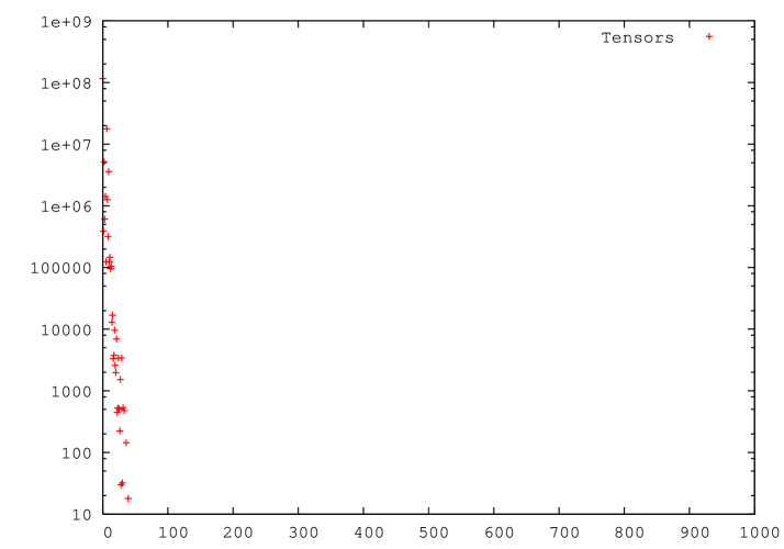
Figure 1: Chiral tensor distribution for all standard model configurations.

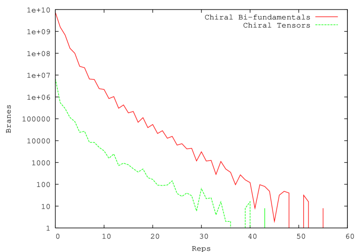
Figure 2: Number of chiral tensors and bi-fundamentals for a selection of branes.

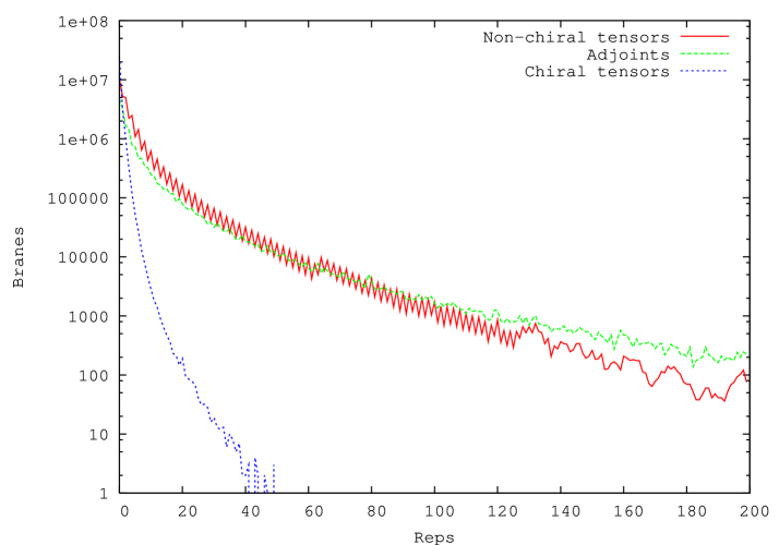
Figure 3: Number of chiral and non-chiral tensors for all single branes.

Note that only a very small fraction of the allowed bottom-up models is actually realized as top-down configurations. This can be explained in part by the fact that the bottom up models can have several chiral tensors instead of chiral bi-fundamentals. In figure (1) we plot the distribution of the number of standard model top-down configurations we have found versus the total number of chiral tensors in the spectrum. This distribution is sharply peaked at zero. This implies that models in which some quarks and leptons are realized as rank-2 tensors are considerably harder to find in the part of the landscape we are exploring here. In itself, this does not mean much for the actual realization of the standard model in our universe. After all, the suppression of models with tensors is by several factors of ten only, and this does not seem very significant in comparison to the total number of models in the landscape.

A partial understanding of this strong chiral tensor suppression can be gained as follows. In fig. (2) we plot for all branes of a sample of 18001 orientifolds the distribution of chiral bi-fundamentals and chiral tensors. On the horizontal axis is the absolute value of the chirality, and on the vertical axis the total number of occurrences. Clearly – and not unexpectedly – the number bi-fundamentals is much greater than the number of chiral tensors. This can be intuitively understood by realizing that a brane has a much bigger chance intersecting with any brane yielding a bi-fundamental than intersecting with one specific brane (namely itself), yielding a chiral tensor.

One can also make an interesting observation regarding the occurrence of chiral tensors in comparison to non-chiral ones. In fig. (3) we list for all branes in all 33012 non-zero tension orientifolds the distribution of chiral and non-chiral tensors (separately for adjoints and the other rank-2 tensors). Note that this includes all branes in all Gepner orientifolds with non-zero-tension O-planes, not just those considered in the present paper. Clearly the chiral distribution falls off much faster than the non-chiral ones.

Although some other qualitative observations can be made, we do really not have a good understanding of the absence of certain models. Hypercharge embeddings with $x=-1/2,~{}3/2$ were not found at all. The full list of 19345 configurations does contain some genuine $x=1$ models, with $x$ fixed to that value by the quark and lepton charges. There is a total of 17 distinct ones (for none of these we found a solution to the tadpole conditions). Only one of these, nr. 2919, has an orthogonal group on the $\bf d$-stack, but it is not identical to one of the simple models written down in section 3.5. It has a Chan-Paton group $U(3)\times U(2)\times U(2)\times O(3)$, with both a C and a D brane on stack c. This model was found a total of 1024 times for just two MIPFs. The purely unitary $x=1$ models 1024 and 2624 occur more frequently. Another noteworthy absence in this class is the type B,B’ model introduced in [4]. These models have a Chan-Paton group $U(3)\times U(2)\times U(1)\times U(1)$, and the type-B model only has bifundamentals, whereas type-B’ has anti-symmetric tensor on $U(2)_{\bf b}$. However, all $x=1$ models we found have a $U(2)$ group on brane c, and all have anti-symmetric tensors both on branes b and c. Some of these are similar to the models of [4], but not identical. Note that the type B,B’ models of [4], in to order to be free of cubic anomalies in the two $U(1)$ factors and the $U(2)$, need $U(2)_{\bf b}$-chiral Higgs pairs and anti-symmetric $U(1)$ tensors, as discussed in section 3.5. This suppresses their statistical likelihood.

Another model proposed in the literature that did not emerge in our search is model C of [7]. This is a $U(3)\times U(2)\times U(1)$ model with three $G_{\rm CP}$-chiral neutrinos appearing as anti-symmetric tensors of $U(2)$. However, model nr 7464 in table (LABEL:tbl:Freq) is similar to it. It has exactly the same structure as model C of [7], after replacing $U(2)$ by $Sp(2)$. Then such neutrinos necessarily become non-chiral, and the anomaly cancellation condition for the $U(2)$ factor becomes irrelevant, increasing the chances of finding an example. Model nr. 7464 occurred only 108 times (and without tadpole solutions). Its presence suggests that there is no fundamental obstacle to finding model C, but that it is simply statistically disfavored. In other situations, replacing $U(2)$ by $Sp(2)$ increases the number of occurrences by factors of about 40 to 80, and hence we would expect at most a few examples of model C. This is consistent with finding none.

On the full list of 19345 models there are 150 of the class $x=*$. All of them are truly orientable, i.e the possibility of having anti-symmetric $U(1)$ tensors that do not contribute massless states does not occur. Only one has Chan-Paton group $U(3)\times U(2)\times U(1)\times U(1)$. It is indeed precisely the model (3.1) shown in section 3. Amazingly this simple model occurs only four times (nr. 17055), and just for one MIPF (and without any tadpole solution to tadpole cancellation). This is especially surprising since there are many other $U(3)\times U(2)\times U(1)\times U(1)$ configurations with only bi-fundamentals that do occur much more frequently, as discussed above. For example nr. 543 in table (LABEL:tbl:Freq) occurs 20176 times. This is a standard “Madrid”-type configuration.

5.5 Higgs, neutrino and mirror distributions

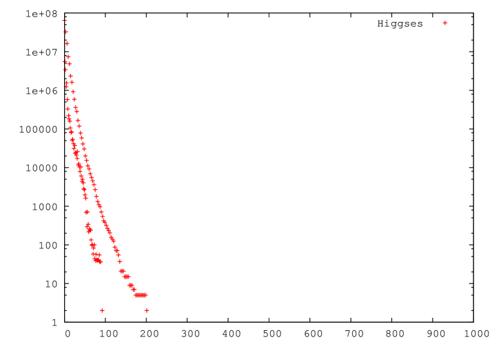
Figure 4: Higgs pair distribution for all standard model configurations.

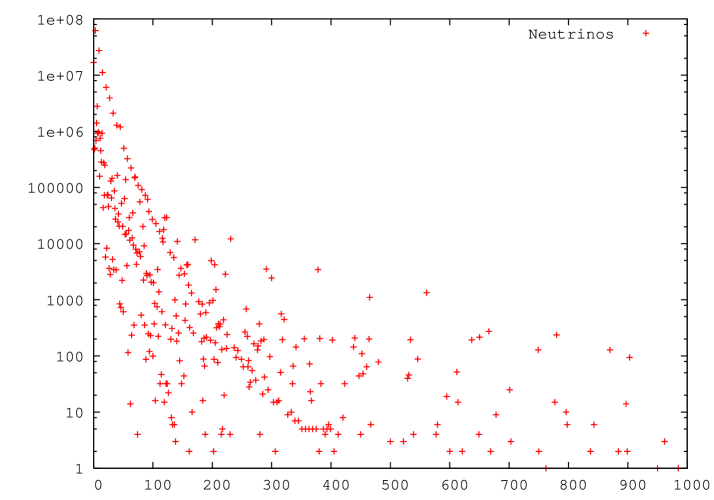
Figure 5: Right-handed neutrino distribution for all standard model configurations.

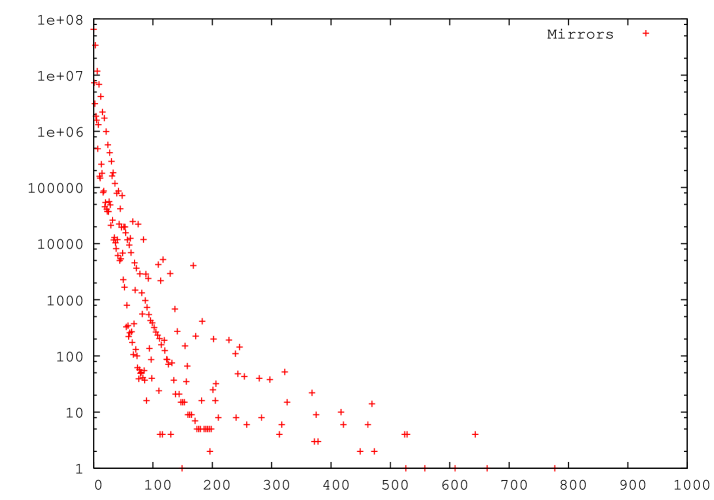
Figure 6: Mirror distribution for all standard model configurations.

Figures (4), (5) and (6) and show the distribution in terms of the number of Higgs, right-handed neutrinos and mirror pairs. On the vertical axis we show the total number of three and four-brane configurations that have a chiral standard model spectrum, plus the number of Higgses/neutrinos/mirrors indicated on the horizontal axis. Just as all data in this section, these numbers refer to brane configurations prior to tadpole cancellation. The Higges/neutrinos/mirrors are $G_{\rm CP}$ chiral but of course $G_{\rm SM}$ non-chiral. In addition to these particles, the massless spectrum may contain $G_{\rm CP}$-non-chiral particles with the same standard model transformation properties. Since we classify models modulo full non-chiral matter, we have no general information about such particles. The mirror count is the total of all mirror pairs of quark and charged lepton weak singlets, as well as quark doublets (in this case mirrors can occur only for $x=\frac{1}{2}$). The Higgs count refers to $(1,2,\frac{1}{2})+(1,2,-\frac{1}{2})$ pairs; for example the MSSM has one such pair. Note that these pairs could also be viewed as lepton doublet mirror pairs. The distinction can be made in models with a well-defined lepton number, but since we are not insisting on that we simply count all such pairs as candidate Higgs. Once one (or more) of these candidates acquires a v.e.v, one may discuss if lepton number violation is absent or acceptably small.

Finally fig. (5) shows the distribution of the total number of standard model singlets in the $G_{\rm CP}$-chiral spectrum.

In all three plots two lines are visible. The top line corresponds to multiplicities that are $0{\rm~{}mod~{}}3$, and the lower to multiplicities that are not $0{\rm~{}mod~{}}3$. The former occur more frequently due to anomaly cancellation and the fact that we require the presence of three chiral families. In some classes of models this imposes a mod 3 constraint on the multiplicities of Higgses, mirror or neutrinos. This feature is clearest in the Higgs plot, because the Higgs is in a definite, and non-trivial standard model representation with few $G_{CP}$ realizations. It is less clear in the neutrino plot, because there are often many ways of making neutrinos. The models with huge numbers of (right-handed) neutrino candidates usually contain a large factor $G_{\bf c}$ or $G_{\bf d}$, with neutrinos coming from rank-2 tensors.

6 Solutions to the tadpole conditions

In this section we present some examples of solutions to complete set of tadpole solutions that we have found. All solutions that we present also satisfy the probe brane constraints for the absence of global anomalies [30], as discussed in [31] for this class of models. We emphasize that we have collected at most two tadpole solutions for each chiral model, one with additional branes, and one without additional branes. This means, for example, that as soon as one solution was found for one of the 9785532 $SU(3)\times SU(2)\times Sp(6)\times U(1)$ models that appears as nr. 1 in table (LABEL:tbl:Freq), no further attempt was made for any of the others with the same chiral spectrum. This is a very different strategy than the one of [12], where all tadpole solutions were collected for models with distinct non-chiral spectra. In the examples below we present the full massless spectrum of the actual tadpole solution, including non-chiral states. The non-chiral states are however specific to the example we present, and solutions with different non-chiral multiplicities for a given chiral multiplicity certainly exist. Indeed, for spectrum nr 2 in table (LABEL:tbl:Freq), which was included in the search presented in [12], more than 100000 non-chirally distinct samples with tadpole solutions were found.

We only present a small selection of the 1900 tadpole solution we have collected. They should be viewed merely as existence proofs of a certain type of model, and not as a statement that one of these is likely to survive further phenomenological constraints. Whenever possible, we present examples without hidden branes, not because we believe these are more viable (indeed, hidden sector branes may be required for a variety of phenomenological reasons), but simply because they can be written down more easily.

6.1 Hypercharge embeddings of the tadpole solutions

Let us first make a few more comments on the models that do or do not occur in the list of 1900 tadpole solutions. We have seen in the previous section that most bottom-up models of section 3 and 4 do not occur on the list of brane configuratios, and it is therefore clear that most are also absent from the list of tadpole solutions (see section 5.4). Furthermore, in many top-down tadpole solutions, the hypercharge appears to be a combination of more than one of the hypercharge embeddings of the bottom-up models in section 4. First consider the “pure” models

• 762 top-down configurations have hypercharge of the form $Y=-{1\over 3}Q_{\bf a}-{1\over 2}Q_{\bf b}$. This is related to a small subclass of bottom-up models in section 4.2.6. In table LABEL:tbl:TableTwo these models have $x=0$ and both ${\bf c}$, ${\bf d}$ branes are of the C type (or are real, or absent).

• 1095 top-down configurations have hypercharge of the form $Y=-{1\over 6}Q_{\bf a}+{1\over 2}Q_{\bf c}-{1\over 2}Q_{\bf d}$ which is related to a subclass of the bottom-up models in section 4.2.4.

The rest of the configurations appear with the hypercharge to be described by two different embeddings. This is due to the contribution of traceless generators in the hypercharge. These “mixed” models are distributed as follows:

• 17 top-down configurations have a combined hypercharge of the type: $Y=-{1\over 3}Q_{\bf a}-{1\over 2}Q_{\bf b}+Q_{\bf d}$ (section 4.2.2 and corresponding to models A,A’ in [4, 23, 32]) and $Y=-{1\over 3}Q_{\bf a}-{1\over 2}Q_{\bf b}$ (section 4.2.6). These are hypercharges with $x=0$ but ${\bf c}$ and ${\bf d}$ branes are of the type C and D, C respectively.

• 2 top-down configurations appear with a combined hypercharge with $x=1$ (section 4.2.3 and corresponding to models B,B’ in [4, 23, 32]), but ${\bf c}$ and ${\bf d}$ branes are of the type C, D and D respectively.

Here we used the hypercharge values as determined from the quark and lepton charges as well as the $Y$-mass condition. The two mixed $x=1$ models mentioned above actually have $x=*$, with $x$ fixed to 1 by the $Y$-mass condition. One of those appears in (LABEL:tbl:TableTwo); the other has too many neutrinos and lies outside the limits used for that table. A total of 20 out of the 1900 tadpole solutions have $x=*$, but $x$ fixed to a non-canonical value by the $Y$-mass condition. Finally there are 4 with $x$ completely unfixed by any condition.

6.2 Notation

The notation of the examples is as follows. Minimal model tensor products are denoted as $(k_{1},\ldots,k_{m})$, where $k_{i}$ is the $SU(2)$ level. Their modular invariant partition functions are labelled by an integer, which is assigned sequentially as they are computed. This labelling can be resolved in terms of more precise data: the simple current subgroup and the rational matrix $X$ defining the MIPF (as defined in [9][10]). We omit these data here, but they are available on request. To help identify the MIPF we will provide the Hodge numbers of the corresponding Calabi-Yau manifold, and the number of singlets that occur in the spectrum of heterotic strings compactified on such a manifold. Orientifolds are also labelled by a sequential integer assigned by the computer program.

Representations are denoted as $(r_{a},...r_{d},...)$, where each entry refers to one of the branes (a, b, c, d and hidden), and $r$ can be $V$ for vector, $A$ for anti-symmetric tensor, $S$ for symmetric tensor and $Adj$ for Adjoint. An asterisk indicates complex conjugation. All representations refer to left-handed fermions. Multiplicities of complex representations are denoted as

$$N\times(r_{a},....)_{M}$$

where $N$ is the total number of times a representation plus its conjugate appears, and $M$ is the chirality, the difference of the multiplicity of the representation that is listed, and its conjugate. The subscript is omitted for non-chiral representations.

6.3 $U(3)\times U(2)\times U(1)$ models

Here we list all tadpole solutions we found with a Chan-Paton group which is exactly $U(3)\times U(2)\times U(1)$ (or less, if some combinations of the unitary phase factors – other than $Y$ – get a mass from axion couplings).

The first two examples are nr. 761 and 762 from the list. They are respectively broken versions of $SU(5)$ and flipped $SU(5)\times U(1)$ unifications, with $SU(5)$ broken by splitting the stack of five branes into three plus two. These models occurred for MIPF 31 of $(1,1,1,1,7,16)$ (there is just one orientifold choice). The $U(3)\times U(2)\times U(1)$ spectrum is

$$3 \times (A,0,0)_{3}$$

$$3 \times (0,A,0)_{3}$$

$$5 \times (V,V,0)_{3}$$

$$25 \times (0,0,S)_{3}$$

$$9 \times (V,0,V)_{-3}$$

$$3 \times (0,V,V)_{-3}$$

$$4 \times (Ad,0,0)$$

$$1 \times (0,Ad,0)$$

$$16 \times (0,0,Ad)$$

$$6 \times (0,0,A)$$

$$8 \times (S,0,0)$$

$$14 \times (V,0,V^{*})$$

$$4 \times (0,V,V^{*})$$

The possible choices for $Y$ are the $SU(5)$ embedding $Y=-\frac{1}{3}Q_{\bf a}+\frac{1}{2}Q_{\bf b}$ and the flipped embedding $Y=\frac{1}{6}Q_{\bf a}+\frac{1}{2}Q_{\bf c}$ for nr. 562 and 561 respectively. In both cases an additional $U(1)$, the independent linear combination of these two, also remains massless.

There is a second, far less standard example of a $U(3)\times U(2)\times U(1)$ model, which occurred for invariant 28 of 441010, orientifold 0. This is nr 16674 on the list, which occurred only six times in total (and only for this MIPF), but against all odds a tadpole solution was found for at least one of the six occurrences. The embedding of $Y$ is as for the flipped $SU(5)$ model above, but only two of the three down quarks are due to anti-symmetric tensors, and there are no anti-symmetric tensors in $U(2)$. Furthermore there are three candidates for Higgs bosons, but unfortunately no symmetry like lepton number to distinguish them from the lepton doublets. This implies that there are no singlet neutrino candidates from the standard model branes, and that with a suitable Higgs boson chosen from the three candidates mentioned above, all up quarks and one of the down quarks can acquire a mass. The exact spectrum is as follows

$$9 \times (0,V,V^{*})_{-3}$$

$$3 \times (0,0,S)_{3}$$

$$6 \times (A,0,0)_{2}$$

$$3 \times (0,0,A)_{1}$$

$$6 \times (0,V,V)_{-6}$$

$$7 \times (V,V,0)_{3}$$

$$7 \times (V,0,V^{*})_{-1}$$

$$3 \times (V,0,V)_{-3}$$

$$3 \times (Ad,0,0)$$

$$6 \times (0,A,0)$$

$$7 \times (0,Ad,0)$$

$$8 \times (0,S,0)$$

$$8 \times (V,V^{*},0)$$

$$4 \times (0,0,Ad)$$

The gauge group is exactly $SU(3)\times SU(2)\times U(1)$, because all abelian gauge bosons other than $Y$ acquire a mass.

Somewhat surprisingly, there were no tadpole solutions for $U(3)\times Sp(2)\times U(1)$ models, even though usually replacing $U(2)$ by $Sp(2)$ greatly increases the frequency of a model.

6.4 Unification

In general we can speak of (partial) unification if some of the stacks a, b, c and d coincide. One can distinguish the following possibilities

1. a = b. In this case the bi-fundamentals that yield quark doublets must necessarily come from anti-symmetric tensors on the combined stack. There must therefore be three anti-symmetric tensors, and the combined gauge group is $U(5)$. Hence this leads to $SU(5)$ GUT models. The $SU(3)$ anti-symmetric tensors can be $u^{c}$ or $d^{c}$ quarks. The first case corresponds to standard $SU(5)$, the second to flipped $SU(5)$. There must be at least one more brane stack to accommodate the anti-quarks of the other charge. Hence these models can be realized with just two stacks.

2. a = c. In this case the weak brane remains separate, but the QCD brane is extended. The best-known example is the Pati-Salam model, where $U(3)_{\bf a}$ is extended with a lepton-number $U(1)$. The Pati-Salam model requires three stacks, but it is possible to realize unifications of this type with just two stacks. An example is (one of the variations of) the $U(6)\times Sp(2)$ discussed below.

3. b = d. In this case the weak brane is part of a larger group. An example is trinification: here $U(2)_{\bf b}$ is embedded in a $U(3)$. Without loss of generality, we may choose stack d as the one that merges with the weak brane. The trinification model then needs one additional brane stack, $U(3)_{\bf c}$. All models in this class must in fact have a third brane stack, in order to get anti-quarks as bi-fundamentals; at least one of the two anti-quarks charges must be realized as a bi-fundamental.

4. a = b = d. An example will be given below.

Here it is assumed that no more branes coincide than those indicated. If c and d coincide this would be regarded as a single stack denoted c. If c coincides with a or b we switch the rôles of c and d. This limits the possibilities to those listed here.

6.4.1 SU(5) models

The following is an example of an $SU(5)$ model. It is item 617 in table (LABEL:tbl:Freq) and despite having a hidden sector, this model has as its gauge group precisely $SU(5)$ and nothing more! The standard model part consists of an $U(5)$ complex stack and a single real $O(1)$ brane. This is needed for the endpoints of the strings yielding the representation $(5^{*})$. In addition this example has one extra $O(1)$ brane that serves as a hidden sector. The example occurs for tensor product (1,4,4,4,4) and MIPF nr. 63 in our classification, which is characterized by Hodge numbers $(h_{21},h_{11})=(7,31)$, and yields 237 singlets if one uses this MIPF to construct a heterotic string. The total number of boundaries is 246. The orientifold is the one with maximal O-plane tension. The precise spectrum is as follows

$$3 \times (A,0,0)_{3}$$

$$11 \times (V,V,0)_{-3}$$

$$8 \times (S,0,0)$$

$$3 \times (Ad,0,0)$$

$$1 \times (0,A,0)$$

$$3 \times (0,V,V)$$

$$8 \times (V,0,V)$$

$$2 \times (0,S,0)$$

$$4 \times (0,0,S)$$

$$4 \times (0,0,A)$$

We emphasize that this just one sample of many such models. There are 16845 configurations of this kind (i.e. with the same first two CP-factors $U(5)\times O(1)$ and the same chiral spectrum). The other 16844 configurations may differ from the one shown here by having, for example, different numbers of $U(5)$ adjoints or $(V,V)$ mirror pairs. Some of these 16845 configurations are identical to the one shown here, because of surviving discrete symmetries of the $(1,4,4,4,4)$ tensor product. But the fact that this chiral spectrum was found for 296 different MIPFs essentially guarantees that many different versions exist.

This model has one hidden sector brane. According to our strategy, outlined in the beginning of this section, none of the remaining models of this type was checked for tadpole cancellation with hidden branes after this tadpole solution was found. All 16845 configurations were checked for tadpole cancellation without hidden branes, and no solutions were found. It is straightforward to re-examine all these 16845 model and check for further possibilities of tadpole cancellation, in order to obtain different non-chiral spectra or different hidden sectors. But there are many other models of potential interest, including many more $SU(5)$ models.

6.4.2 Flipped SU(5) models

The simplest flipped $SU(5)$ we found occurs for for invariant 52 of (1,4,4,4,4), orientifold 0, with characteristics (3,51,253). It solves all tadpole equations with just two brane stacks, the minimal number needed to realize flipped $SU(5)$. The full Chan-Paton group is $U(5)\times U(1)$, and the spectrum is

$$11 \times (0,S)_{3}$$

$$3 \times (A,0)_{3}$$

$$5 \times (V,V)_{-3}$$

$$8 \times (S,0)$$

$$9 \times (Ad,0)$$

$$5 \times (0,Ad)$$

$$4 \times (0,A)$$

$$12 \times (V,V^{*})$$

In terms of (a, b, c, d) branes this model is of the form $U(3)_{a}\times U(2)_{b}\times U(1)_{c}$ with a $=$ b and no d brane, and $Y=\frac{1}{6}(1,0,3)$. The way the $U(1)$ anomalies cancel is noteworthy. Per family, there are five $U(1)$ anti-vector representations, contribution -5 to the cubic anomaly. This anomaly is cancelled by a symmetric tensor, which contributes $+5$ in a $U(1)$ theory. The chiral part of the spectrum yields exactly the standard model spectrum, with 3 right-handed neutrinos from the three chiral symmetric tensors. There are no $G_{\rm CP}$-chiral Higgs candidates.

This is model nr. 2880 in table (LABEL:tbl:Freq). As explained earlier, such a flipped $SU(5)$ model always has a standard $SU(5)$ counterpart, because the masslessness of the extra $U(1)$ of flipped $SU(5)$ is an additional constraint not needed for standard $SU(5)$. This is model nr 2881 in table (LABEL:tbl:Freq).

To the best of our knowledge, these are the first exact chiral, supersymmetric $SU(5)$ and flipped $SU(5)$ models in the literature. Their chiral spectrum, directly obtained in string theory, without postulating further Higgs effects or non-perturbative physics, is exactly $3\times(10)+3\times(5^{*})$. By contrast, the models found in [33] contain additional $(15)$’s of $SU(5)$. The models found recently in [34] have $G_{\rm CP}$ mirror pairs of $(5)$ and $(5^{*})$, which must be made massive by postulating an additional Higgs mechanism breaking part of the additional gauge symmetry. We emphasize that the mirror pairs shown above in the explicit spectrum are non-chiral with respect to the full Chan-Paton group, and hence require no gauge symmetry breaking to acquire a mass.

In addition, the model shown above is obviously the simplest one possible, apart from the $U(5)\times O(1)$ of the previous subsection, if one could find a realization without hidden sector.

However, both the standard and the flipped $SU(5)$ model have a serious problem with either the $(u,c,t)$ or $(d,s,b)$ Yukawa coupling. We will discuss this in detail in section 7.2.

For other work discussing aspects of (flipped) $SU(5)$ model building along similar lines, see [35][36] [37],[33][38][34]. For other issues in $SU(5)$ model building with branes and the associated problems see [39], [40].

6.4.3 Pati-Salam models

The simplest Pati-Salam model is nr. 4 on the list, and is therefore one of the most frequent ones. A tadpole solution was found for invariant 57 of (2,10,10,10), orientifold 3. The gauge group is $U(4)\times Sp(2)\times Sp(2)$, and the spectrum is as follows

$$5 \times (V,0,V)_{-3}$$

$$3 \times (V,V,0)_{3}$$

$$2 \times (Ad,0,0)$$

$$2 \times (0,A,0)$$

$$7 \times (0,0,A)$$

$$4 \times (A,0,0)$$

$$2 \times (0,S,0)$$

$$5 \times (0,0,S)$$

$$7 \times (0,V,V)$$

The embedding of $Y$ is as $Y=\frac{1}{6}Q_{\bf a}-\frac{1}{2}Q_{\bf d}+W_{\bf c}$, where $W_{\bf c}=\frac{1}{2}\sigma_{3}$. Brane a and d are unified to $U(4)$.

The following model is of interest because it is a $U(4)\times U(2)\times U(2)$ Pati-Salam model that satisfies all tadpole conditions without hidden branes, because it has some chiral rank-2 tensors in its spectrum, and because it occurs for a MIPF related to the “quintic” Calabi-Yau, namely MIPF 6 of (3,3,3,3,3), the trivial orientifold (the only one possible). It is nr. 4825 on the list (LABEL:tbl:Freq). It has precisely one $G_{\rm CP}$ chiral MSSM Higgs pair, plus a $G_{\rm CP}$-chiral charged lepton mirror pair, and four right-handed neutrinos. There is one massless $U(1)$ in addition to $Y$, namely the diagonal combination of the phase factors of the $U(2)$’s. The Chan-Paton group is $U(4)\times U(2)\times U(2)$, and the representations are

$$3 \times (V,0,V^{*})_{-1}$$

$$2 \times (V,0,V)_{-2}$$

$$1 \times (0,0,S)_{1}$$

$$5 \times (0,A,0)_{1}$$

$$5 \times (V,V^{*},0)_{1}$$

$$6 \times (V,V,0)_{2}$$

$$3 \times (0,V,V)_{-1}$$

$$4 \times (0,S,0)$$

$$4 \times (S,0,0)$$

$$3 \times (Ad,0,0)$$

$$5 \times (0,Ad,0)$$

$$1 \times (0,0,Ad)$$

$$2 \times (0,V,V^{*})$$

There also exist a broken version of this model, with $U(4)$ split into $U(3)\times U(1)$ already in the exact string theory. This is nr. 7053 in (LABEL:tbl:Freq).

There is also a $U(4)\times U(2)\times U(2)$ Pati-Salam model (nr. 153) which has a standard, purely bi-fundamental spectrum. For this model we only found a tadpole solution with hidden branes, which is a bit too complicate to display here. It has a hidden sector group $U(6)\times U(2)^{3}\times O(2)^{2}\times Sp(2)$.

Orientifolds exhibiting a Pati-Salam realization of the SM have been considered before, [41, 42, 43]. Bottom-up configurations, investigating also gauge couplings and the issue of masses, have been also considered, [44, 45].

6.4.4 Trinification models

Trinification models are built out of three factors $SU(3)$ with purely bi-fundamental matter. At first sight this would seem to be an ideal configuration for intersecting brane models, but in fact it is surprisingly rare.

In a genuine trinification model the generator $Y$ is embedded in $SU(3)_{\bf a}\times SU(3)_{\bf b}\times SU(3)_{\bf d}$ as $Y=\frac{1}{6}W_{\bf b}-\frac{1}{3}W_{\bf d}$, where $W_{\bf b}=W_{\bf d}=\rm{diag}(1,1,-2)$. However, a trinification model is in our classification a model with $x=*$, which allows arbitrary shifts in the choices of $Y$. For any other choice of $Y$ this implies that a combination of the unitary phases contributes to $Y$. The canonical choice of $Y$ has no contribution from $U(3)_{\bf a}$ and hence would correspond to $x=\frac{1}{3}$, a non-standard choice. Although the quark and lepton charges do not fix $x$, this may be done by the zero $Y$-mass condition.

In table (LABEL:tbl:Freq) three distinct models with this characteristic appear. The most frequent one, nr. 225, has a fixed value of $Y$ of the canonical trinification type, with $x=\frac{1}{3}$. However, we did not find solutions to the tadpole conditions for any of these 71328 models. The second one, nr. 1125, has a completely free $Y$; even the zero mass condition for $Y$ does not fix it. This type of model occurred 6432 times and for at least one of these we found a solution to all tadpole conditions. The third one, nr. 12327, occurred only 24 times, and for none of them the tadpoles were solved. It has $Y$ fixed to a value which does not correspond to standard trinification ($x=\frac{1}{2}$).

The aforementioned tadpole solution occurred for invariant 11 of tensor product $(1,16,16,16)$, orientifold 0 (with $(h_{21},h_{11},S)=(9,111,481)$). It has a rather large hidden sector gauge group $U(3)\times U(3)\times U(3)\times O(4)\times O(2)\times U(6)\times U(12)\times O(12)\times U(12)\times O(4)$, with respect to which the spectrum is as follows:

$$3 \times (V,V,0,0,0,0,0,0,0,0)_{3}$$

$$3 \times (V,0,V,0,0,0,0,0,0,0)_{-3}$$

$$3 \times (0,V,V^{*},0,0,0,0,0,0,0)_{-3}$$

$$1 \times (0,0,0,V,0,V,0,0,0,0)_{-1}$$

$$1 \times (0,0,0,0,0,S,0,0,0,0)_{1}$$

$$5 \times (0,0,0,0,0,0,0,V,V,0)_{1}$$

$$3 \times (0,0,0,0,0,0,0,0,S,0)_{1}$$

$$1 \times (0,0,0,0,0,A,0,0,0,0)_{-1}$$

$$2 \times (0,0,0,0,0,0,0,0,A,0)_{-2}$$

$$1 \times (0,0,0,V,0,0,0,0,V,0)_{1}$$

$$1 \times (0,0,0,0,V,0,0,0,V,0)_{1}$$

$$1 \times (0,0,0,0,0,V,0,V,0,0)_{1}$$

$$1 \times (0,0,0,0,0,V,0,0,V,0)_{-1}$$

$$1 \times (0,0,0,0,0,0,V,V,0,0)_{1}$$

$$1 \times (0,0,0,0,0,0,V,0,V,0)_{-1}$$

$$1 \times (0,0,0,0,0,V,0,0,0,V)_{-1}$$

$$1 \times (0,0,0,V,V,0,0,0,0,0)$$

$$1 \times (0,0,0,0,S,0,0,0,0,0)$$

$$1 \times (0,0,0,0,0,Ad,0,0,0,0)$$

$$1 \times (0,0,0,0,0,0,Ad,0,0,0)$$

$$3 \times (0,0,0,0,0,0,0,S,0,0)$$

$$3 \times (0,0,0,0,0,0,0,0,Ad,0)$$

$$1 \times (0,0,0,0,0,0,0,0,0,S)$$

$$2 \times (0,0,0,0,V,V,0,0,0,0)$$

$$1 \times (0,0,0,0,V,0,0,V,0,0)$$

$$2 \times (0,0,0,0,0,V,0,0,V^{*},0)$$

$$2 \times (0,0,0,0,0,0,V,0,V^{*},0)$$

$$1 \times (0,0,0,0,V,0,0,0,0,V)$$

$$1 \times (0,0,0,0,0,0,0,V,0,V)$$

Bottom-up trinification models and their phenomenology has been discussed in [28].

6.5 Curiosities

6.5.1 A non-standard $U(3)\times Sp(2)\times U(1)\times U(1)$ model

The following spectrum was found for 17, orientifold 2 of the tensor product $(2,2,2,6,6)$. It has a hidden sector group $U(2)$ which is completely decoupled from all massless matter: both OH as HH matter is absent. The main reason for listing it here is however that it is an alternative to the standard lepton-number conserving configurations. This is nr. 4996 in (LABEL:tbl:Freq).

The full Chan-Paton group is $U(3)\times Sp(2)\times U(1)\times U(1)\times U(2)$, with the following spectrum

$$3 \times (V,V,0,0,0)_{3}$$

$$3 \times (0,0,V,V,0)_{-3}$$

$$1 \times (V,0,0,V^{*},0)_{-1}$$

$$2 \times (V,0,V,0,0)_{-2}$$

$$2 \times (0,V,0,V,0)_{2}$$

$$3 \times (V,0,0,V,0)_{-1}$$

$$3 \times (0,V,V,0,0)_{1}$$

$$2 \times (V,0,V^{*},0,0)_{-2}$$

$$1 \times (0,0,V,V^{*},0)_{1}$$

$$4 \times (A,0,0,0,0)$$

$$2 \times (0,0,0,S,0)$$

The $Y$-embedding is $Y=\frac{1}{6}Q_{\bf a}-\frac{1}{2}Q_{\bf c}-\frac{1}{2}Q_{\bf d}$. There is no additional massless $U(1)$ factor from the standard model branes (we did not compute the mass of the abelian factor of $U(2)$). Note that the endpoints of the quarks and lepton doublet bi-fundamentals are distributed over the c and d branes, making it impossible to assign a lepton number. Indeed, there are perturbatively allowed lepton-number violating couplings of the type $(Q,L,d^{c})$ or $(L,L,l^{c})$, but further CFT computations would be needed to verify if these couplings do indeed occur. The $G_{\rm CP}$-chiral spectrum has no Higgs candidates and just one right-handed neutrino candidate.

We have also found a similar model with $U(2)_{\bf b}$ instead of $Sp(2)_{\bf b}$, and a slightly more complicated hidden sector. It combines two features not encountered together in [12]: a group $U(3)\times U(2)\times U(1)\times U(1)$ of which only $U(1)_{Y}$ survives as an abelian vector boson. Unfortunately this is achieved at a price that is presumably to high: the reason is that lepton number cannot be written in terms of the brane charges. As a result, no linear combination of $B$ and $L$ is anomaly free. Model nr. 1725 is of the same kind, but with $Sp(2)$ replaced by $U(2)$. A tadpole solution exists for that model with an $O(2)\times O(2)$ hidden sector.

6.5.2 A $U(6)$ model

The following examples were found for invariant 79 of (1,4,4,4,4), orientifold 0, corresponding to an orientifold with Calabi-Yau characteristics (6,60,288). These are exact standard model realizations with just two branes stacks, a complex and a real one. In fact, this single model can accommodate the standard model spectrum in three distinct ways. The unified gauge group is $U(6)\times Sp(2)$. The spectrum is as follows

$$9 \times (A,0)_{3}$$

$$9 \times (V,V)_{-3}$$

$$8 \times (Ad,0)$$

$$1 \times (0,A)$$

$$7 \times (0,S)$$

The first standard model realization is obtained by splitting $U(6)$ so that the full (a,b,c,d) configuration becomes $U(3)_{\bf a}\times U(2)_{\bf b}\times Sp(2)_{\bf c}\times U(1)_{\bf d}$, with a, b and d belonging to the same stack. The choice of $Y$ is $\frac{1}{6}(1,0,0,-3)+W_{\bf c}$, where $W_{\bf c}$ is the diagonal Pauli matrix $\frac{1}{2}\sigma_{3}$ in $Sp(2)_{\bf c}$. The first term of $Y$ is part of the non-abelian group $SU(4)$ formed by the a and d branes, and hence automatically massless. If the breaking pattern is interpreted as $U(6)\rightarrow U(5)\times U(1)\rightarrow U(3)_{\bf a}\times U(2)_{\bf b}\times U(1)_{\bf c}$ the second step is a flipped $SU(5)$ model; if the breaking is interpreted as $U(6)\rightarrow U(4)\times U(2)\rightarrow U(3)_{\bf a}\times U(2)_{\bf b}\times U(1)_{\bf c}$ the intermediate stage is Pati-Salam-like.

The second realization appears if we split $U(6)$ in the same way as $U(3)_{\bf a}\times U(2)_{\bf b}\times Sp(2)_{\bf c}\times U(1)_{\bf d}$, but now with $Y$ is $(-\frac{1}{3},\frac{1}{2},0,0)$. This amounts to a standard $SU(5)$ embedding of the standard model. The $Sp(2)$ group does not contribute to $Y$ in this case.

Finally there is the possibility of using $Sp(2)$ as a b-type stack for the weak interactions. To achieve this we split $U(6)$ as $U(3)_{\bf a}\times U(3)_{\bf c}$, and write $Y$ as $\frac{1}{6}(1,0,-1)+W_{\bf c}$, where $W_{\bf c}$ is the $SU(3)$-generator $(\frac{2}{3},-\frac{1}{3},-\frac{1}{3})$. There is no d-stack.

All three models have three candidate Higgs pairs an three down quarks mirror pairs, as well as six right-handed neutrino candidates, which are chiral with respect to $U(6)$. The first two are nrs. 1886 and 1887 in table (LABEL:tbl:Freq), and the third one is nr. 1888.

7 Phenomenological implications and the problem of masses

In this section we will address, in a rather general fashion, some phenomenological aspects of SM brane configurations. In particular, we are going to discuss the problem of masses in theories with anti-quarks in the antisymmetric representation of SU(3), as well as the nature of potential family symmetries and neutrino masses.

7.1 Antisymmetric anti-quarks and the problem of quark masses

There is a generic potential phenomenological problem, when one of the anti-quarks originate from anti-symmetrized strings starting and ending on the color branes. Although for SU(3), $\vbox{\vbox{\offinterlineskip\vbox{\hrule height=0.3pt\hbox{\vrule height=5.92001pt,width=0.3pt,depth=1.47997pt\hbox to7.4pt{\hfil}\vrule height=5.92001pt,width=0.3pt,depth=1.47997pt} \hrule height=0.3pt}\vspace{-\y@linethick} \vbox{\hrule height=0.3pt\hbox{\vrule height=5.92001pt,width=0.3pt,depth=1.47997pt\hbox to7.4pt{\hfil}\vrule height=5.92001pt,width=0.3pt,depth=1.47997pt} \hrule height=0.3pt}\vspace{-\y@linethick} }}={\overline{\vbox{\vbox{\offinterlineskip\vbox{\hrule height=0.3pt\hbox{\vrule height=5.92001pt,width=0.3pt,depth=1.47997pt\hbox to7.4pt{\hfil}\vrule height=5.92001pt,width=0.3pt,depth=1.47997pt} \hrule height=0.3pt}\vspace{-\y@linethick} }}}}$, the antisymmetric representation has charge 2, under the U(1)_a instead of the -1 for ${\overline{\vbox{\vbox{\offinterlineskip\vbox{\hrule height=0.3pt\hbox{\vrule height=5.92001pt,width=0.3pt,depth=1.47997pt\hbox to7.4pt{\hfil}\vrule height=5.92001pt,width=0.3pt,depth=1.47997pt} \hrule height=0.3pt}\vspace{-\y@linethick} }}}}$.

We are using the language of left-handed fermions where

$$\bar{\psi}^{c}_{R}\equiv\psi_{L}^{T}~{}C\;\;\;,\;\;\;C^{-1}\gamma^{\mu}C=-(\gamma^{\mu})^{T}$$ (7.15)

where $C$ is the charge conjugation matrix. $\bar{\psi}^{c}_{R}$ is a right-handed Weyl fermion transforming in the same representation of the gauge group as $\psi_{L}$. The mass terms can be therefore be written in terms of fermion bilinears

$$\bar{\psi}^{c}_{R}~{}\chi_{L}+h.c.$$ (7.16)

Consider the (color singlet) quark mass operator $(\bar{Q}^{c})^{I}_{a}q^{J}$, where $Q$ denotes the quarks (3,2) and $q$ stands for the anti-quarks in the               of SU(3). $I,J$ indices from now on will collectively indicate any other index except color and weak indices. $a$ is a weak doublet index. $({\bar{Q}^{c}})^{I}q^{J}$ transforms as a weak doublet, and has charge 3 under U(1)_a. Therefore it must be coupled to a weak Higgs doublet that should also carry charge -3. However a single field in orientifolds cannot carry charge -3. Therefore, a product of scalar fields must be involved. The minimal case involves scalars $H^{I}_{a}$ transforming as ($\bar{3}$,2,-1) under $SU(3)\times SU(2)\times U(1)_{\bf a}$ and $A^{K}$ transforming as ($\overline{\vbox{\vbox{\offinterlineskip\vbox{\hrule height=0.3pt\hbox{\vrule height=5.92001pt,width=0.3pt,depth=1.47997pt\hbox to7.4pt{\hfil}\vrule height=5.92001pt,width=0.3pt,depth=1.47997pt} \hrule height=0.3pt}\vspace{-\y@linethick} \vbox{\hrule height=0.3pt\hbox{\vrule height=5.92001pt,width=0.3pt,depth=1.47997pt\hbox to7.4pt{\hfil}\vrule height=5.92001pt,width=0.3pt,depth=1.47997pt} \hrule height=0.3pt}\vspace{-\y@linethick} }}}$,1,-2). The putative mass term would then be

$$\delta{\cal L}_{1}=h_{I,J,K,L}~{}((\bar{Q}^{c})^{I}_{a}Q^{J})(H^{Ka}A^{L})$$ (7.17)

where the parentheses indicate the color contractions. Non-minimal couplings would include

$$\delta{\cal L}_{2}=\tilde{h}_{I,J,K,L}~{}((\bar{Q}^{c})^{I}_{a}Q^{J})G^{a}(F^{K}A^{L})\;\;\;,\;\;\;\delta{\cal L}_{2}=\hat{h}_{I,J,K,L,M}~{}((\bar{Q}^{c})^{I}_{a}Q^{J})G^{a}(F^{K}F^{L}F^{M})$$ (7.18)

where $G^{a}$ is a standard Higgs (weak doublet), $F^{I}$ transforms as ($\bar{3}$,1,-1) and in the last case an antisymmetric color coupling of three triplets is implied. There might also be additional constraints, due to the fact that the $F_{I}$ scalars come from strings that have one end point in the $c,d$ branes.

The crucial point is that in order to generate the quark mass terms, the scalar combinations in (7.17) and (7.18) must acquire expectation values. This necessarily implies that the scalars $H^{Ia}$ or $F^{I}$ or $A^{I}$ must have vevs, and this necessarily breaks the color symmetry to SU(2)_color (along with $U(1)_{\bf a}$ of course). This seems incompatible with current data. Moreover, this conclusion is robust, and is valid independent of the presence or not of supersymmetry.

There are two a priori possibilities in order to avoid the previous impasse. The first is that non-perturbative effects break the associated global symmetry. It is well known that anomalous U(1)’s have always mixed anomalies with non-abelian groups. Therefore, there are always gauge instantons and their string theory generalization, that violate the global symmetry non-perturbatively (see [46]). There are two distinct possibilities, but only one is relevant here: the case when the non-abelian gauge group is unbroken at low energy . This is indeed the case with the color group. In this case only terms involving a minimum number of fermions can be generated. This minimum number is required in order to soak up the zero modes of instantons. It is always larger than two in realistic situations. Therefore, it is not relevant for generating mass terms for the fermions.

The other option is to start from a higher gauge-group, that is eventually broken to the color SU(3), giving masses to the standard quarks. Let us entertain first the case of SU(4). We should use the following facts, [47]: A scalar in the adjoint of SU(4) obtaining a vev may break the gauge symmetry $SU(4)\to SU(2)\times U(2)$ or $SU(3)$ depending on the type of vev. A scalar in the          , breaks the gauge symmetry as $SU(4)\to O(4)$ or $SU(3)$ depending on the type of vev. A scalar in the               breaks the gauge symmetry as $U(4)\to Sp(4)$ or $SU(4)\to SU(2)$ depending on the type of vev. Finally a scalar transforming in the (4,2) of $SU(4)\times SU(2)$ breaks the symmetry as $SU(4)\times SU(2)\to SU(3)$, or $SU(2)\times SU(2)$ depending on the type of vev. Although this may be acceptable from the color point of view, the breaking of the weak SU(2) group is acceptable only if the bi-fundamental scalar carries the correct SM hypercharge.

Therefore the scalar vevs that preserve an SU(3) color subgroup SU(4) transformations are

$${\rm adjoint}\sim{\Phi_{\alpha}}^{\beta}\sim\left(\matrix{1&0&0&0\cr 0&0&0&0\cr 0&0&0&0\cr 0&0&0&0\cr}\right)\sim\phi_{\alpha\beta}\sim\vbox{\vbox{\offinterlineskip\vbox{\hrule height=0.3pt\hbox{\vrule height=5.92001pt,width=0.3pt,depth=1.47997pt\hbox to7.4pt{\hfil}\vrule height=5.92001pt,width=0.3pt,depth=1.47997pt\hbox to7.4pt{\hfil}\vrule height=5.92001pt,width=0.3pt,depth=1.47997pt} \hrule height=0.3pt}\vspace{-\y@linethick} }}$$ (7.19)

$$\vbox{\vbox{\offinterlineskip\vbox{\hrule height=0.3pt\hbox{\vrule height=5.92001pt,width=0.3pt,depth=1.47997pt\hbox to7.4pt{\hfil}\vrule height=5.92001pt,width=0.3pt,depth=1.47997pt} \hrule height=0.3pt}\vspace{-\y@linethick} }}\sim F_{\alpha}\sim\left(\matrix{1\cr 0\cr 0\cr 0\cr}\right)\;\;\;,\;\;\;(4,2)\sim H^{a}_{\alpha}\sim\left(\matrix{1&0&0&0\cr 0&1&0&0\cr}\right)$$ (7.20)

The last operator breaks also to the SU(2). and they must be aligned. This poses strong constraints on the appropriate scalar potentials. In particular, no antisymmetric vev is allowed.

We may now go through the potential mass terms and show that none is acceptable. We suppress all other indices but SU(4) color and write

$${\cal O}_{1}=(\bar{Q}^{c})_{\alpha}q_{\beta\gamma}F^{\alpha}F_{I}^{\beta}F_{J}^{\gamma}\;\;\;,\;\;\;{\cal O}_{2}=(\bar{Q}^{c})_{\alpha}q_{\beta\gamma}\phi^{\alpha\beta}F^{\gamma}$$ (7.21)

$${\cal O}_{3}=\epsilon^{\alpha\beta\gamma\delta}(\bar{Q}^{c})_{\alpha}q_{\beta\gamma}F_{\delta}~{}\epsilon_{\alpha^{\prime}\beta^{\prime}\gamma^{\prime}\delta^{\prime}}F_{I}^{\alpha^{\prime}}F_{J}^{\beta^{\prime}}F_{K}^{\gamma^{\prime}}F_{L}^{\delta^{\prime}}$$ (7.22)

where a lower SU(4) index transforms as        and an upper one as $\overline{\vbox{\vbox{\offinterlineskip\vbox{\hrule height=0.3pt\hbox{\vrule height=5.92001pt,width=0.3pt,depth=1.47997pt\hbox to7.4pt{\hfil}\vrule height=5.92001pt,width=0.3pt,depth=1.47997pt} \hrule height=0.3pt}\vspace{-\y@linethick} }}}$. The operators ${\cal O}_{i}$ moreover transform as weak doublets and have $U(1)_{\bf a}$ charge zero. There are also operators which involve adjoint scalars but they have no new features. It is straightforward to check that operators ${\cal O}_{1,2}$ fail to provide mass operators for any of the fermions after the breaking $SU(4)\to SU(3)$ by the vevs in (7.19) and (7.20). Operator ${\cal O}_{3}$ gives masses to the standard SU(3) quarks, but leaves the rest massless. One of the fundamentals in ${\cal O}_{i}$ can be substituted with the $H^{a}_{\alpha}$ scalar. This will provide a weak singlet. Moreover as we have seen this vev breaks $SU(4)\times SU(2)\to SU(3)$, and if the hypercharge of the scalar is 1/2, then it will provide at the same time the proper, electroweak symmetry breaking. However, the same considerations as above indicate than no reasonable mass terms are generated.

The final case to be considered is the possibility to include a scalar vev in the antisymmetric representation, $R^{\alpha\beta}$. In this case we must start from SU(5), which the vev will break to SU(3). Upon choosing a convenient basis this vev is

$$\vbox{\vbox{\offinterlineskip\vbox{\hrule height=0.3pt\hbox{\vrule height=5.92001pt,width=0.3pt,depth=1.47997pt\hbox to7.4pt{\hfil}\vrule height=5.92001pt,width=0.3pt,depth=1.47997pt} \hrule height=0.3pt}\vspace{-\y@linethick} \vbox{\hrule height=0.3pt\hbox{\vrule height=5.92001pt,width=0.3pt,depth=1.47997pt\hbox to7.4pt{\hfil}\vrule height=5.92001pt,width=0.3pt,depth=1.47997pt} \hrule height=0.3pt}\vspace{-\y@linethick} }}\sim R^{\alpha\beta}\sim\left(\matrix{\phantom{-}0&1&0&0&0\cr-1&0&0&0&0\cr\phantom{-}0&0&0&0&0\cr\phantom{-}0&0&0&0&0\cr\phantom{-}0&0&0&0&0\cr}\right)$$ (7.23)

We also assume that there are fundamentals $F^{\alpha}$ with a vev in the 4 and 5 directions, so that it does not break SU(3) further. Then we may write the following operators

$${\cal O}_{4}=(\bar{Q}^{c})_{\alpha}q_{\beta\gamma}F^{\alpha}R^{\beta\gamma}\;\;\;,\;\;\;{\cal O}_{5}=\epsilon^{\alpha\beta\gamma\delta\epsilon}(\bar{Q}^{c})_{\alpha}q_{\beta\gamma}\rho_{\delta\epsilon}~{}\epsilon_{\alpha^{\prime}\beta^{\prime}\gamma^{\prime}\delta^{\prime}\epsilon^{\prime}}F^{\alpha^{\prime}}R^{\beta^{\prime}\gamma^{\prime}}R^{\delta^{\prime}\epsilon^{\prime}}$$ (7.24)

The operator ${\cal O}_{4}$ provides masses for the various singlets after the breaking. Operator ${\cal O}_{5}$ provides masses for the standard quarks. However the two extra triplets emerging from the               of SU(5) will remain massless.

It therefore seems that orientifold models with anti-quarks in antisymmetric representations are phenomenologically untenable.

7.2 Masses in SU(5) and flipped SU(5) vacua

The case of standard U(5) group deserves special attention. The SM particles are in the antisymmetric representation $\psi^{\alpha\beta}$ as well as the anti-fundamental, $\psi_{\alpha}$. The minimal set of scalar needed for symmetry breaking is an adjoint ${\Phi^{\alpha}}_{\beta}$ whose expectation value ${\rm diag}(2V,2V,2V,-3V,-3V,-3V)$ breaks $SU(5)\to SU(3)\times SU(2)\times U(1)_{Y}$ and a fundamental, $H^{\alpha}$ whose expectation value $(0,0,0,0,v)$ breaks $SU(2)\times U(1)_{Y}\to U(1)_{em}$ The standard mass terms

$${\cal O}_{1}\sim(\bar{\psi}^{c})_{\alpha}\psi^{\alpha\beta}H_{\beta}\;\;\;,\;\;\;{\cal O}_{2}\sim\epsilon_{\alpha\beta\gamma\delta\epsilon}(\bar{\psi}^{c})^{\alpha\beta}\psi^{\gamma\delta}H^{\epsilon}$$ (7.25)

give masses to all SM fermions. However here, ${\cal O}_{2}$ which gives masses to up-type quarks is not allowed, since it carries charge +5 under the overall U(1) of the U(5). This charge can be cancelled by multiplication by $\epsilon^{\alpha\beta\gamma\delta\epsilon}H^{I}_{\alpha}H^{J}_{\beta}H^{K}_{\gamma}H^{K}_{\delta}H^{L}_{\epsilon}$, which however requires the presence of 5 fundamental Higgs scalars with vevs that are aligned, and of the order of the electroweak scale. However, such a mass is suppressed by a factor $\prod_{I=1}^{5}{v_{I}\over M_{s}}$. Since all $v_{I}\lesssim M_{Z}$, we obtain an unacceptable suppression factor of $10^{-50}$. The other possibility is the presence of symmetric or antisymmetric scalars that acquire vevs. An antisymmetric vev cannot preserve the $SU(3)\times U(1)_{em}$ group of low energy physics. A symmetric one, $R^{\alpha\beta}$ is fine provided it is aligned as in (7.19). Its vev $\tilde{V}$ must be smaller than the EW vev as it contributes to the W,Z masses. Again, although ${\cal O}_{2}$ can be neutralized, it gives too small a contribution to up quark masses. There are new operators we may write now like

$${\cal O}_{3}\sim(\bar{\psi}^{c})_{\alpha\beta}\psi_{\gamma\delta}R^{\alpha\gamma}R^{\beta\delta}$$ (7.26)

However, such an operator does not contribute to fermion masses.

We can imagine of two non-perturbative loopholes to the previous arguments. A first non-perturbative possibility is based on breaking the offending U(1) symmetry by a vacuum condensate. An example will be a Chan-Paton group that contains U(5)$\times$ SO(5)$\times$ SO(5), and we have extra scalars (denoted Q${}_{\alpha}^{A}$) in the representation (V,V,0)+(V^∗,0,V), so that the U(5) anomalies cancel. If the dynamics is favorable, we may imagine that one of the SO(5)’s creates a composite out of five scalars, of the form

$$\epsilon^{\alpha\beta\gamma\delta\epsilon}\epsilon_{ABCDE}Q^{A}_{\alpha}Q^{B}_{\beta}\cdots Q^{E}_{\epsilon},$$ (7.27)

where $\alpha,\beta,\cdots$ are SU(5) indices and $A,B,\cdots$ SO(5) indices. If the condensate gets a vev at the GUT scale, but not the individual fields $Q^{A}_{\alpha}$, it breaks the U(1) of U(5), and upon coupling to the U(5) quarks and leptons can generate the appropriate masses. It should be however mentioned that such a dynamical setup seems unlikely.

The final possibility, is a non-perturbative breaking of the overall (anomalous) U(1) symmetry because of instantons. In the case of unbroken SU(5) symmetry, the numerous zero modes of the instantons do not produce mass terms. They could though upon symmetry breaking. Whether mass terms can be generated in this case requires a detailed analysis of the instanton induced terms and will not be attempted here.

7.3 Family symmetries

We have allowed extra non-abelian groups to participate in the local SM collection of branes. In particular standard model particles are charged under such groups. This setup is very reminiscent of the idea of family symmetries. The purpose of the introduction of family symmetry in the past was to explain/organize the existence of three generations and the hierarchy of masses of the SM particles. There are two relevant questions in this context:

(a) Can such symmetries play the role of family symmetries? Can they help achieve realistic mass matrices for the SM particles?

(b) Are there cases where the presence of such symmetries forbids realistic mass matrices?

In following we will make some comments on these two questions. Although our setup is reminiscent of family symmetries, it incorporates a radical departure from that idea as well. The reason is that the quark (3,2) states, cannot be charged under any other gauge symmetry. This is unlike any other family symmetry introduced in the literature. Since the quarks are necessarily not-charged under such symmetries, there are non-trivial considerations concerning the potential mass matrices and the existence of realistic patterns.

At this stage, we are not fully prepared to calculate three and higher point couplings in the superpotential. We can however derive some selection rules on couplings, especially renormalizable ones (three-point couplings) that are allowed by the gauge symmetries. Such selection rules can have non-trivial consequences because

(i) Extra non-abelian symmetries, although broken, may be more or less constraining, due to the possible symmetry breaking vevs.

(ii) The presence of several (anomalous) U(1)s provides further constraints, especially if the corresponding global symmetries remain intact in perturbation theory.

From now on we will call for concreteness the non-abelian group $G$ distinct from SU(2) and S(3), the family symmetry group. Let us consider the case where the anti-quarks $q_{i}$ transform in a non-trivial representation $R$ of the group $G$. Then the potential mass term $(\bar{Q}^{c})^{I,a}q_{i}$ transform as a doublet of SU(2) and as R of $G$ (I is a extra index labeling the three quark generations, while $a$ is a weak doublet index). At the cubic level the existence of a scalar $\Phi_{a}^{i}$ transforming in the (2,R) of $SU(2)\times G$, gives rise to the Yukawa coupling

$$(\bar{Q}^{c})^{I,a}q_{i}~{}\Phi_{a}^{i}$$ (7.28)

Up to base change there are two types of vevs for $\Phi$, [47]. The first type breaks the symmetry $SU(2)\times G\to G^{\prime}$, with $G^{\prime}=O(N-1)$ if $G=O(N)$ and $G^{\prime}=SU(N-1)$ if $G=SU(N)$. Therefore, the electroweak symmetry is broken while the family symmetry is not fully broken. For this to be realistic, further vev’s should break both the $U(1)_{Y}$ symmetry and the leftover family symmetry. The pattern then becomes complicated and deserves a detailed study. The second type breaks $SU(2)\times G\to SU(2)\times G^{\prime}$ with $G^{\prime}=O(N-2)$ if $G=O(N)$ and $G^{\prime}=SU(N-2)$ if $G=SU(N)$. Here the family symmetry is completely broken if $N=2$. This is the case for example of a Pati-Salam group. If there is a leftover family symmetry, further symmetry breaking is necessary. The $\Phi$ vev identifies the weak and the G index and provides a mass matrix for quarks that is degenerate. The existence of several copies of $\Phi$ does not improve the situation.

We can contemplate higher dimension terms involving a weak double $H^{a}$ and a scalar $\Phi_{i}$ in the fundamental of $G$

$$(\bar{Q}^{c})^{I,a}q_{i}~{}H^{a}\Phi^{i}$$ (7.29)

In such a case a vev of $\Phi$ of the order of $M_{s}$ will give a mass matrix of order of the electroweak scale but it will be degenerate. Moreover the $G$ symmetry is partly broken. Several scalars $H^{I}_{i}$ with couplings

$${g_{IJ}\over M_{s}}~{}(\bar{Q}^{c})^{I,a}q_{i}~{}H^{a}\Phi^{i}_{J}$$ (7.30)

could fare better. First non-aligned expectation values can break a larger portion or all of the G group. Second, for generic couplings $g_{IJ}$ the mass matrix after electroweak breaking will be non-degenerate. Therefore, in this case, a reasonable non-zero mass matrix is viable.

There are more complicated possibilities of the occurrence of quasi-family symmetries and the charge assignments of SM particles under them. We have studied in some indicative examples, the relevant issues present. A full study of all possibilities is a major task and it will not be undertaken here.

7.4 Neutrino masses

In our search we have not explicitly constrained the presence of anti-neutrinos. A priori, any SM singlet fermion can play that role. Of course, for a realistic pattern of masses to emerge, important constraints on the interactions are appropriate.

There are two mechanisms that so far have been successful in producing neutrino masses of acceptable magnitude. The first, relies on the see-saw mechanism and is appropriate for vacua with high values of the string scale. An important ingredient for its operations is that lepton number is not conserved. Moreover at least two (and typically three) antineutrinos are necessary for accommodating present data. As we have discussed earlier, the presence of lepton number cannot be directly tracked until a formal separation of doublets into leptons and Higgses is possible. Therefore in this context, the question of neutrino masses remains a question to be addressed in concrete string ground states.

The second mechanism involves a brane wrapping one (or several) large dimensions and is necessarily operative in string vacua with a low string scale. In this context the neutrinos mix with antineutrinos emerging from the “bulk” brane , and the masses are suppressed by the volume of large dimensions. For this mechanism to succeed large Majorana masses should be forbidden. Therefore it is important that lepton number is a good symmetry. Moreover, the minimal implementation involves a single antineutrino and its KK tower of states and leads to predictions marginally compatible with current data [23]. More comfortable constructions involve at least two antineutrinos.

8 Dependence of the results on the Calabi-Yau topology

Table LABEL:tableCY lists the MIPFs for which the standard model spectrum was found, and how often it occurred. The table is ordered according to standard model frequency, that is the total number of standard model configurations divided by the total number of three and four brane configurations. Note that this does not take into account tadpole cancellation, since we have not systematically solved the tadpole conditions for all standard model configurations. Column 2 gives the MIPF id-number using the same sequential labelling used in [12]. We can provide further details on these MIPFs on request. To help identifying them, we list in columns 3,4 and 5 the resulting heterotic Calabi-Yau spectrum (Hodge numbers and the number of $E_{6}$ singlets). In columns 6,7 and 8 we list the total number of configurations for each value of $x$. The last column gives the frequency.

Table 7: Standard model success rate for various MIPFs.

Tensor product	MIPF	$h_{11}$	$h_{12}$	Scalars	$x=0$	$x=\frac{1}{2}$	$x=*$	Success rate
(1,1,1,1,7,16)	30	11	35	207	1698	388	0	$2.1\times 10^{-3}$
(1,1,1,1,7,16)	31	5	29	207	890	451	0	$1.35\times 10^{-3}$
(1,4,4,4,4)	53	20	20	150	2386746	250776	0	$4.27\times 10^{-4}$
(1,4,4,4,4)	54	3	51	213	5400	5328	4248	$3.92\times 10^{-4}$
(6,6,6,6)	37	3	59	223	0	946432	0	$2.79\times 10^{-4}$
(1,1,1,1,10,10)	50	12	24	183	1504	508	36	$2.63\times 10^{-4}$
(1,1,1,1,10,10)	56	4	40	219	244	82	0	$2.01\times 10^{-4}$
(1,1,1,1,8,13)	5	20	20	140	328	27	0	$1.93\times 10^{-4}$
(1,1,1,1,7,16)	26	20	20	140	157	14	0	$1.72\times 10^{-4}$
(1,1,7,7,7)	9	7	55	276	7163	860	0	$1.59\times 10^{-4}$
(1,1,1,1,7,16)	32	23	23	217	135	20	0	$1.56\times 10^{-4}$
(1,4,4,4,4)	52	3	51	253	110493	8303	0	$1.02\times 10^{-4}$
(1,4,4,4,4)	13	3	51	250	238464	168156	0	$1.01\times 10^{-4}$
(1,1,1,2,4,10)	44	12	24	225	704	248	0	$1.01\times 10^{-4}$
(1,1,1,1,1,2,10)	21	20	20	142	2	1	0	$1.00\times 10^{-4}$
(1,1,1,1,1,4,4)	124	0	0	78	729	0	0	$9.8\times 10^{-5}$
(4,4,10,10)	79	7	43	215	0	57924	0	$9.39\times 10^{-5}$
(4,4,10,10)	77	5	53	232	0	1068926	0	$8.29\times 10^{-5}$
(1,4,4,4,4)	77	3	63	248	0	1024	0	$8.12\times 10^{-5}$
(4,4,10,10)	74	9	57	249	0	1480812	0	$8.06\times 10^{-5}$
(1,1,1,1,1,2,10)	24	20	20	142	0	0	6	$7.87\times 10^{-5}$
(1,2,4,4,10)	67	11	35	213	0	14088	1008	$7\times 10^{-5}$
(1,1,1,1,5,40)	5	20	20	140	303	36	0	$6.73\times 10^{-5}$
(2,8,8,18)	8	13	49	249	0	1506776	0	$6.03\times 10^{-5}$
(1,1,7,7,7)	7	22	34	256	2700	68	0	$5.5\times 10^{-5}$
(1,4,4,4,4)	78	15	15	186	20270	6792	0	$5.39\times 10^{-5}$
(2,8,8,18)	28	13	49	249	0	670276	0	$5.25\times 10^{-5}$
(1,2,4,4,10)	75	5	41	212	304	580	244	$4.87\times 10^{-5}$
(1,1,7,7,7)	17	10	46	220	1662	624	108	$4.76\times 10^{-5}$
(2,2,2,6,6)	106	3	51	235	0	201728	0	$4.74\times 10^{-5}$
(1,1,1,16,22)	7	20	20	140	244	19	0	$4.67\times 10^{-5}$
(1,2,4,4,10)	65	6	30	196	0	1386	0	$4.41\times 10^{-5}$
(4,4,10,10)	66	6	48	223	0	61568	0	$4.33\times 10^{-5}$
(1,4,4,4,4)	57	4	40	252	0	266328	58320	$4.19\times 10^{-5}$
(1,4,4,4,4)	80	7	37	200	0	1968	1408	$4.15\times 10^{-5}$
(6,6,6,6)	58	3	43	207	0	190464	0	$3.93\times 10^{-5}$
(1,1,1,1,10,10)	36	20	20	140	266	26	6	$3.82\times 10^{-5}$
(1,1,1,4,4,4)	125	12	24	214	351	0	0	$3.62\times 10^{-5}$
(4,4,10,10)	14	4	46	219	0	114702	0	$3.3\times 10^{-5}$
(1,1,1,1,10,10)	33	20	20	140	47	5	0	$3.21\times 10^{-5}$
$\ldots$								$\ldots$
(3,3,3,3,3)	6	21	17	234	0	192	0	$6.54\times 10^{-6}$
$\ldots$								$\ldots$
(3,3,3,3,3)	4	5	49	258	0	24	0	$8.17\times 10^{-7}$
$\ldots$								$\ldots$
(3,3,3,3,3)	2	49	5	258	6	27	6	$1.65\times 10^{-9}$
$\ldots$								$\ldots$

The complete table has 1639 cases with non-zero frequency. Therefore we only present the top of the table here, which starts with a frequency as high as $.2\%$. The last three entries are modular invariants of the tensor $(3,3,3,3,3)$, corresponding to the quintic. They occur much further down the list, but are shown here because the quintic is a well-studied Calabi-Yau manifold. The lowest non-zero frequency we encountered is $3.5\times 10^{-12}$ (for a total of 4 configurations found).

In column 2 an asterisk indicates that at least one tadpole solution was found for that MIPF in [12]. Note that we did not perform an exhaustive search for tadpole solutions in the present work. Indeed, if all brane configurations occurring for a given MIPF are of a type for which the tadpoles have already been solved before (for a different MIPF), no further attempts are made to solve them. Therefore we cannot make definitive conclusions about the non-existence of tadpole solutions for a given MIPF from our present results.

Note the presence of models with Hodge numbers $(20,20)$. The corresponding Calabi-Yau manifolds are in fact of the form $K_{3}\times T_{2}$. There is also a case with $h_{11}=h_{12}=0$, which is in fact a torus compactification. The fact that these are (partly) torus compactifications is not in contradiction with the fact that the spectrum is chiral. Each MIPF can be thought of as a an extension of the chiral algebra of the original tensor product, modified by an automorphism. This extension may lead to a non-chiral torus compactification. However the boundary states that are admitted are a complete set with respect to the original unextended chiral algebra, which always corresponds to a chiral compactification (except for five non-chiral tensor products that we do not consider). Hence a non-chiral bulk extension may have chiral boundary states. It is possible that the $K_{3}\times T_{2}$ models are related to models discussed in ([48]); this will require further investigation. In any case we did not find tadpole solutions for any of these torus or $K_{3}\times T_{2}$ models (but again with the caveat that we did not search for them exhaustively).

We did find tadpole solutions for one of the MIPFs of the quintic, namely MIPF nr. 6. These solutions are the broken and unbroken Pati-Salam $U(4)\times U(2)\times U(2)$ models discussed above.

Acknowledgements

We would like to thank I. Antoniadis, M. Bianchi, R. Blumenhagen, M. Douglas, F. Gmeiner, G. Honecker, D. Lüst, and H. Verlinde for discussions. This work was partially supported by ANR grant NT05-1-41861, INTAS grant, 03-51-6346, RTN contracts MRTN-CT-2004-005104 and MRTN-CT-2004-503369, CNRS PICS 2530 and 3059 and by a European Excellence Grant, MEXT-CT-2003-509661. P. A. was supported by the research program “Pythagoras II” (grant 70-03-7992) of the Greek Ministry of National Education, partially funded by the European Union. The work of A.N.S. has been performed as part of the program FP 52 of the Foundation for Fundamental Research of Matter (FOM), and the work of T.P.T.D. and A.N.S. has been performed as part of the program FP 57 of FOM. The work A.N.S. has been partially supported by funding of the Spanish “Ministerio de Ciencia y Tecnología”, Project BFM2002-03610.

Appendices

Appendix A The unbiased search algorithm

We introduce the following notation (in the following $a,b,\ldots$ are generic boundary state labels, not to be confused with the specific labels a, b for the QCD, weak and other standard model branes)

$$N_{ab}=\sum_{i}A^{i}_{~{}ab}\chi_{i}(m=0,L)$$

where $A^{i}_{~{}ab}$ are the unoriented annulus coefficients and $\chi_{i}(m=0,L)$ is the character of representation $i$, restricted to massless, left-handed fermions. The boundary conjugates of $a$ and $b$ are denoted by $a^{c}$ and $b^{c}$ . If we consider two complex boundaries $a$ and $b$, there is $a$ total of four quantities relevant for the massless spectrum, namely $N_{ab}$ , $N_{ab^{c}}$, $N_{a^{c}b}$ and $N_{a^{c}b^{c}}$ . The chiral information is contained in two quantities, namely

$$\Gamma_{ab}=N_{ab}-N_{a^{c}b^{c}}$$

and

$$\Delta_{ab}=N_{ab^{c}}-N_{a^{c}b}$$

If either $a$ or $b$ are real, we set $\Delta=0$. If both $a$ and $b$ are real $\Gamma=\Delta=0$. Furthermore we define the chiral numbers of anti-symmetric and symmetric tensors

$$A_{a}=\frac{1}{2}(N_{aa}-N_{aa^{c}}-M_{a}+M_{a^{c}})$$

and

$$S_{a}=\frac{1}{2}(N_{aa}-N_{aa^{c}}+M_{a}-M_{a^{c}})$$

where $M$ is the Moebius contribution

$$M_{a}=\sum_{i}M^{i}_{~{}a}\chi_{i}(m=0,L)\ .$$

Our search procedure is as follows

1. Consider all orientifold choices that have non-zero tension. We will label them by an integer $\ell$. This sequential label corresponds to some choice of the discrete parameters of the RCFT, called “Klein bottle currents” and “crosscap signs” [8]. The sign of the tension of the corresponding O-plane is a free parameter in RCFT constructions, and we choose it negative. We denote its value as $T_{O}^{\ell}$.

2. For each $\ell$, consider all candidates for brane a subject to the conditions

   1. Brane a is complex.

   2. The brane tension $T_{\bf a}$ satisfies $6T_{\bf a}+T^{\ell}_{O}<0$, because the complete configuration must satisfy the dilaton tadpole condition $\sum_{x}T_{x}+T^{\ell}_{O}=0$, and all $T_{x}$ are positive. This is needed in order to accommodate further branes.

   3. There are no chiral symmetric tensors.

3. For each $\ell$ and a, consider all candidates for brane b that satisfy the following conditions

   1. The CP group associated with b is not orthogonal.

   2. The brane tension $T_{\bf b}$ satisfies $6T_{\bf a}+2T_{\bf b}+T^{\ell}_{O}<0$, if b is real, $6T_{\bf a}+4T_{\bf b}+T^{\ell}_{O}<0$ if b is complex.

   3. There are three chiral bi-fundamentals $(3,2)$. These are only counted chirally, i.e additional mirror pairs are allowed. If brane b is complex, the chiral total of $(3,2)$ and $(3,2^{*})$ must be three.

   4. There are no chiral symmetric tensors. This is the an application of the condition mentioned in section 2, that $R^{\rm chir}_{CP}$ should not yield anything more exotic than mirrors. It is not absolutely essential here, but it gives a useful early limitation on the number of solutions.

4. For each $\ell$, a and b consider all candidates c that satisfy:

   1. Brane c is allowed at least once by the dilaton tension constraint.

   2. We need weak singlet anti-quarks. They can come from anti-symmetric tensors of brane a or from bi-fundamentals between brane a and either branes c or d. Since the anti-symmetric tensors can have only one charge, at least three anti-quarks must come from bi-fundamentals. There is no a priori ordering between branes c and d. To prevent double-counting, we will impose the condition that brane c must provide more anti-quarks plus mirrors than brane d. More precisely, we will impose the condition $N_{{\bf c}}(|\Gamma_{{\bf a}{\bf c}}|+|\Delta_{{\bf a}{\bf c}}|)\geq N_{{\bf d}}(|\Gamma_{{\bf a}{\bf d}}|+|\Delta_{{\bf a}{\bf d}}|)$. This ordering condition can only be imposed once we have determined branes c and d as well as their CP multiplicities $N_{{\bf c}}$ and $N_{{\bf d}}$, but at this stage it already implies that ($|\Gamma_{{\bf a}{\bf c}}|+|\Delta_{{\bf a}{\bf c}}|)>0\ .$

5. Given $\ell$ a, b and c there may be a value for $N_{\bf c}$ (the CP multiplicity of brane c) and a hypercharge choice so that the standard model is already obtained for just three stacks. However, in general a fourth stack is needed (even if there is a valid three-stack solution we will continue looking for a fourth one). Hence we consider all labels d that satisfy:

   1. At least one of the stacks b, c and d is complex. Otherwise it would be impossible to obtain chiral leptons.

   2. At least one of the quantities $S_{\bf d}$ , $A_{\bf d}$ , $\Gamma_{{\bf a}{\bf d}}$, $\Gamma_{{\bf b}{\bf d}}$ , $\Gamma_{{\bf c}{\bf d}}$ , $\Delta_{{\bf a}{\bf d}}$, $\Delta_{{\bf b}{\bf d}}$ , and $\Delta_{{\bf c}{\bf d}}$ is non-zero. Otherwise brane d can be regarded as part of the hidden sector.

6. Now we have collected an orientifold and four branes a, b, c, d and we have to determine the CP multiplicities of the last two branes. Because, by assumption, any further branes are in the hidden sector and cannot contribute chiral states to the four CP groups, all cubic anomalies must now cancel. This gives at least two and at most four equations for the two quantities $N_{\bf c}$ and $N_{\bf d}$ . The following things can happen:

   1. There are two independent equations that fix $N_{\bf c}$ and $N_{\bf d}$. Both are positive integers, and are even for symplectic groups. Now we can move on to the next stage, and compute the Y-charge combination (see below).

   2. The equations are inconsistent, do not have positive integer solutions, or have a solution with an odd CP multiplicity for a symplectic group. In all these cases the configuration $(\ell,{\bf a},{\bf b},{\bf c},{\bf d})$ must be rejected.

   3. There is only one independent equation. This means that only a linear combination $f_{\bf c}N_{\bf c}+f_{\bf d}N_{\bf d}$ is fixed. If this happens we consider all values of $N_{\bf d}$ or $N_{\bf c}$ (if $f_{\bf c}=0$) between 1 and the maximum allowed by the dilaton tadpoles, and attempt the next stage (computing $Y$) for all of them.

   4. There is no equation at all. This means that all anomalies cancel independent of $N_{\bf c}$ and $N_{\bf d}$. This can only happen if $A_{\bf a}=6$. If $A_{\bf a}\not=6$, there must be chiral bi-fundamentals giving rise to anti-quarks, and their contribution to the $SU(3)$ anomaly depends on $N_{\bf c}$ or $N_{\bf d}$, or both. In this case we consider all allowed values of $N_{\bf c}$ as well as $N_{\bf d}$ and attempt to determine $Y$.

7. The next step is to compute the standard model $Y$-charge. In general it is a linear combination of the form $Y=\sum_{\alpha}t_{\alpha}Q_{\alpha}+W_{\bf c}+W_{\bf d}$, where $Q_{\alpha}$ is the $U(1)$ charge of one of the unitary brane stacks, with $\alpha=({\bf a},{\bf b},{\bf c},{\bf d})$. Real stacks have $Q_{\alpha}=0$. The last two terms are simple Lie-algebra generators in the CP-factors of branes c and d, in other words generators of $SU(N)$, $O(N)$ or $Sp(N)$. They can be brought to diagonal form and may therefore be parametrized as traceless diagonal matrices, which in the case of $O(N)$ and $Sp(N)$ must have equal numbers of eigenvalues of opposite sign. We first determine the coefficients $t_{\alpha}$. We do this by solving one of the following sets of equations:

   • Trace Equations: These are obtained by taking the trace for each of the $SU(3)\times SU(2)$ representations $(3,2)$, $(3^{*},1)$, $(2,1)$ and $(1,1)$. On the phenomenological side, any non-chiral mirror pairs do not contribute to these traces, and on the string theory side $W_{\bf c}$ and $W_{\bf d}$ do not contribute. Therefore this gives four equations for at most four variables $t_{\alpha}$.

   • Axion Equations: Require absence of axion-Y bilinear couplings. This gives a condition for every axion, and yields in general far more conditions than there are variables. Note that $W_{\bf c}$ and $W_{\bf d}$ do not couple to any axions. Since we want rational solutions $t_{\alpha}$ and since the axion couplings are real numbers, the solutions have to be converted to rational numbers of the form $p/q$. We perform that conversion assuming $|q|\leq 1024$.

   • Exact Charge Equations: Write down equations for the actual charges (rather than the traces) for each non-zero coefficient $A,S,\Gamma$ or $\Delta$. We write these equations for the maximal eigenvalue in the c and d sectors, i.e. for the maximal eigenvalue of $x_{\bf c}=t_{c}Q_{\bf c}+W_{\bf c}$ or $x_{\bf d}=t_{d}Q_{\bf d}+W_{\bf d}$. The right hand side of such an equation must be a valid (mirror) quark or lepton charge, and is determined up to at most an integer $0,\pm 1$. These linear equations can be solved, and limit $x_{\bf c}$ and $x_{\bf d}$ to a definite range of integers and half-integers. To determine $t_{\bf c}$ (and analogously $t_{\bf d}$) we consider all possible multiplicities of the eigenvalue $W_{\bf c}^{\rm max}$, between $1$ and $N_{\bf c}$. Given this multiplicity, and the fact that $W_{\bf c}$ is traceless, we can determine $t_{\bf c}$. Taking into account all these possibilities (the integer ambiguities and the number of maximal eigenvalues) then gives a set of possible variables for $t_{c}$ and $t_{d}$.

   These methods are used successively as needed. The first is the simplest and usually sufficient, and only in rare cases the third method is needed. The $Y$-mass constraint is in any case checked as a condition, if it was not used as equation. Note that the exact charge equations cannot fix all $t_{\alpha}$ if the brane configuration is orientable. In that case these equations have a one-dimensional kernel, and only the axion equations might fully determine $t_{\alpha}$. To summarize, we have following possibilities:

   1. The trace equations completely fix all $t_{\alpha}$. In that case the axion-$Y$ bilinear couplings are computed for this particular $Y$. If they all vanish, we move on to the next step.

   2. The equations do not fix all $t_{\alpha}$. In that case we combine the trace equations with the axion equations.

   3. The trace and axion equations still do not all fix $t_{\alpha}$. In that case we use the exact charge equations to determine the missing coefficient(s) up to a finite set of rational numbers.

   4. The trace plus axion equations do not determine all $t_{\alpha}$ completely, and neither do the exact charge equations. In this case both sets of equations have a non-trivial kernel and there are two possibilities:

      1. The kernel vector of the exact charge equations is in the kernel of the trace and axion equations. This means that we can add a set of coefficients $x_{\alpha}$ to $t_{\alpha}$ without affecting the quark and lepton charges, nor the axion couplings. This is a genuine ambiguity, which cannot be resolved by any conditions at our disposal. We fix this ambiguity by setting one of the missing coefficients to a chosen “canonical” value ($\frac{1}{6}$, 0,$-\frac{1}{2}$, $-\frac{1}{2}$ for $t_{a},\ldots t_{c}$ respectively).

      2. The kernel vector of the exact charge equations is not in the kernel of the trace and axion equations. In this case the equations can be solved by combining them. There is a minor complication due to the fact that the exact charge equations have a range of rational numbers as their right hand side. To deal with this we consider a set of rational values $p/q$ for the missing $t_{\alpha}$. For $q$ we use the smallest common multiple of $24,N_{\bf c}$ and $N_{\bf d}$, and we allow all values for $p$ so that $-1\leq p/q\leq 1$. Since the kernels of the two set of equations do not overlap, there will be at most a few solutions.

   All possibilities described above do actually occur.

8. Determining $W_{\bf c}$ and $W_{\bf d}$, given $t_{\alpha}$. This is now easy, because the eigenvalues of these generators must lower or raise the value of $Y$ to an allowed quark or lepton charge. Hence at most two distinct eigenvalues are allowed. Since the generators must be traceless, this fixes them completely. If the c or d groups are orthogonal or symplectic, the two eigenvalues must be equal in number and opposite. Note that for $SU(3)\times SU(2)$ singlets we allow three charges, $0,\pm 1$, but if there is an equal number of charges $+1$ and $-1$ this just adds non-chiral pairs. This is a degeneracy, that can be fixed by setting all paired charges to $0$. Hence also in this case at most two distinct $W_{\bf c}$ or $W_{\bf d}$ eigenvalues are needed.

9. Finally we count the quarks and leptons, to check that the correct particle multiplicities are obtained.

There is some potential over-counting in the procedure, due to the following reasons

1. If the b-brane is complex, one can interchange b and ${\bf b}^{c}$

2. The choice of c and d is interchangeable.

3. The choice of c and ${\bf c}^{c}$ is interchangeable.

4. The choice of d and ${\bf d}^{c}$ is interchangeable.

These degeneracies are fixed as follows. The first one can be dealt with by requiring that there are more chiral representations $(3,2)$ than $(3,2^{*})$. Since their total must be three, they cannot be equal. The second one can be fixed by requiring that brane c produce a larger total number of anti-quarks than brane d, i.e. $N_{{\bf c}}(|\Gamma_{{\bf a}{\bf c}}|+|\Delta_{{\bf a}{\bf c}}|)\geq N_{{\bf d}}(|\Gamma_{{\bf a}{\bf d}}|+|\Delta_{{\bf a}{\bf d}}|)$. If that still yields equality, we require that brane c produce more chiral anti-quarks than brane d. A few further constraints of this type may be used to fix the ambiguity completely. To fix the conjugation ambiguities of the c and d branes we require that certain chiral quantities associated with these branes are positive.

Appendix B Gauge coupling ranges of various hypercharge embeddings

The range of possible variation of the string scale in orientifold vacua is a very interesting question. Its extreme values, close to the Planck scale on th high side and in the TeV range for the low side, both have phenomenological merits and problems. It is the purpose of this appendix to give a rough idea on the range of string scale values allowed in various hypercharge embeddings described in this paper. Although, branes $\bf c$ and $\bf d$ may be non-abelian, we will assume here for simplicity that they carry U(1) factors. Moreover we will allow their associated gauge couplings to vary in the perturbative regime between zero and one.

Using the string prediction for the hypercharge embedding, we can evaluate the hypercharge coupling at the string scale. In the standard normalization of the non-abelian couplings the U(1) coupling normalization is $g_{i}^{2}/2i$ where $i$ is the number of “colors”:

$${1\over g_{Y}^{2}}={6x_{\bf a}^{2}\over g_{\bf a}^{2}}+{4x_{\bf b}^{2}\over g_{\bf b}^{2}}+{2x_{\bf c}^{2}\over g_{\bf c}^{2}}+{2x_{\bf d}^{2}\over g_{\bf d}^{2}}$$ (B.31)

where $x_{i}$ are the coefficients in (3.3). The couplings of the $U(1)_{\bf a}$ and $U(1)_{\bf b}$ are directly related to the strong and weak coupling constants. We take the $U(1)_{\bf c}$, $U(1)_{\bf d}$, couplings to be a priori independent.

The one-loop coupling evolution is given by:

$${1\over\alpha_{i}(m)}={1\over\alpha_{i}(M_{Z})}-{b_{i}\over 2\pi}\ln{m\over M_{Z}}$$ (B.32)

where $\alpha_{i}=g^{2}_{i}/4\pi$ and:

$$\alpha_{3}(M_{Z})=0.1172(\pm 0.003)~{}~{} ~{}~{}~{}~{}~{}~{}\alpha_{em}(M_{Z})=1/127.934$$ ,

$$M_{Z}=0.0911876~{}TeV~{}~{} ~{}~{}~{}~{}~{}~{}\sin^{2}\theta_{Z}=0.23113$$ , (B.33)

where $\sin^{2}\theta_{Z}=\alpha_{em}(M_{Z})/\alpha_{2}(M_{Z})$.

Inserting (B.32) in (B.31), we have

$$\ln{M_{Z}\over M_{s}}={-{1\over\alpha_{Y}(M_{Z})}+{6x_{\bf a}^{2}\over\alpha_{\bf a}(M_{Z})}+{2x_{\bf b}^{2}\over\alpha_{\bf b}(M_{Z})}+\sum_{i}{2x_{\bf i}^{2}\over\alpha_{\bf i}(M_{s})}\over-{b_{Y}\over 2\pi}+{6x_{\bf a}^{2}b_{\bf a}\over 2\pi}+{2x_{\bf b}^{2}b_{\bf b}\over 2\pi}}$$ (B.34)

The equation above expresses the string scale as a function of the three SM couplings $\alpha_{3}$, $\alpha_{2}$, $\alpha_{Y}$ evaluated at the $Z$-mass, the values of the $U(1)_{c,d}$ couplings at the string scale, the one-loop $\beta$-function coefficients and the coefficients of the hypercharge embedding $x_{i}$. We use the one-loop $\beta$-functions for non-supersymmetric and supersymmetric SM to be:

$$(b_{3},b_{2},b_{Y})_{SM}=(-7,-3,7)~{}~{}~{},~{}~{}~{}~{}~{}~{}~{}(b_{3},b_{2},b_{Y})_{MSSM}=(-3,1,11)~{}.$$ (B.35)

Moreover we put a uniform threshold at the supersymmetric case around 1 TeV.

By varying the U(1) couplings $\alpha_{i={\bf c,d}}$ between zero and one we obtain a range of allowed values for $M_{s}$. In particular, by choosing small values for $\alpha_{i={\bf c,d}}$ arbitrarily small values for the string scale are obtained. The maximum value for the string scale occurs for values of the couplings at the boundary of the strong coupling region that we take by convention to be $\alpha_{{\bf c}}=\alpha_{{\bf d}}=1$.

The maximum value of the string scale $M_{s}$ is obtained for strongly coupled $U(1)$ branes. It is interesting to evaluate this maximum value for all models, since it provides an upper bound for the string scale and makes models with the maximum $M_{s}$ in the few TeV range particularly attractive.

The indicative maximum value of the string scale is tabulated below for the various choices of hypercharge embeddings. In column 1 we list the value of $x$; One of the $x=\frac{1}{2}$ models has a brane of type F on position d, as indicated. $SU(5)$ models are those with $x=0$ and one or two extra branes of type C.

We observe that only two hypercharge embeddings do not allow a large string scale.

$x$		$Y~{}~{}~{}~{}~{}~{}~{}~{}~{}~{}~{}~{}~{}$	$M_{max}$ No-SUSY (TeV)	$M_{max}$ SUSY (TeV)
0		$-\frac{1}{3}Q_{\bf a}-\frac{1}{2}Q_{\bf b}+Q_{\bf d}$	$2.133\times 10^{10}$	$7.168\times 10^{12}$
1		$\frac{2}{3}Q_{\bf a}+\frac{1}{2}Q_{\bf b}+Q_{\bf c}$	$1419.91$	433114.
${1\over 2}$		$\frac{1}{6}Q_{\bf a}+\frac{1}{2}Q_{\bf c}-\frac{1}{2}Q_{\bf d}$	$1.041\times 10^{31}$	$5.314\times 10^{21}$
${1\over 2}$	(F)	$\frac{1}{6}Q_{\bf a}+\frac{1}{2}Q_{\bf c}-\frac{3}{2}Q_{\bf d}$	$4.797\times 10^{29}$	$5.975\times 10^{20}$
0	(C)	$-\frac{1}{3}Q_{\bf a}-\frac{1}{2}Q_{\bf b}$	$5.024\times 10^{10}$	$2.043\times 10^{13}$
$-{1\over 2}$		$-\frac{5}{6}Q_{\bf a}-Q_{\bf b}-\frac{1}{2}Q_{\bf c}+\frac{3}{2}Q_{\bf d}$	$1.041\times 10^{31}$	$5.314\times 10^{21}$
${3\over 2}$		$\frac{7}{6}Q_{\bf a}+Q_{\bf b}+\frac{3}{2}Q_{\bf c}+\frac{1}{2}Q_{\bf d}$	$3.802\times 10^{-5}$	$5.828\times 10^{-10}$

References

- [1] L. Susskind, “The anthropic landscape of string theory,” [ArXiv:hep-th/0302219].
- [2] A. N. Schellekens, “The landscape ’avant la lettre’,” [ArXiv:physics/0604134].
- [3] F. Denef and M. R. Douglas, “Computational complexity of the landscape. I,” [ArXiv:hep-th/0602072].
-
[4]
I. Antoniadis, E. Kiritsis and T. N. Tomaras,
“A D-brane alternative to unification,”
Phys. Lett. B 486 (2000) 186
[[ArXiv:hep-ph/0004214]];
“D-brane Standard Model,” Fortsch. Phys. 49 (2001) 573 [ArXiv:hep-th/0111269]. - [5] G. Aldazabal, L. E. Ibanez, F. Quevedo and A. M. Uranga, “D-branes at singularities: A bottom-up approach to the string embedding of the standard model,” JHEP 0008 (2000) 002 [ArXiv:hep-th/0005067].
- [6] L. E. Ibanez, F. Marchesano and R. Rabadan, “Getting just the standard model at intersecting branes,” JHEP 0111 (2001) 002 [ArXiv:hep-th/0105155].
- [7] I. Antoniadis and S. Dimopoulos, “Splitting supersymmetry in string theory,” Nucl. Phys. B 715 (2005) 120 [ArXiv:hep-th/0411032].
-
[8]
J. Fuchs, L. R. Huiszoon, A. N. Schellekens, C. Schweigert and J. Walcher,
“Boundaries, crosscaps and simple currents,”
Phys. Lett. B 495 (2000) 427
[ArXiv:hep-th/0007174]. - [9] B. Gato-Rivera and A. N. Schellekens, Commun. Math. Phys. 145 (1992) 85.
- [10] M. Kreuzer and A. N. Schellekens, Nucl. Phys. B 411, 97 (1994) [arXiv:hep-th/9306145].
- [11] T. P. T. Dijkstra, L. R. Huiszoon and A. N. Schellekens, “Chiral supersymmetric standard model spectra from orientifolds of Gepner models,” Phys. Lett. B 609 (2005) 408 [ArXiv:hep-th/0403196].
-
[12]
T. P. T. Dijkstra, L. R. Huiszoon and A. N. Schellekens,
“Supersymmetric standard model spectra from RCFT orientifolds,”
Nucl. Phys. B 710 (2005) 3
[ArXiv:hep-th/0411129]. - [13] C. Angelantonj, M. Bianchi, G. Pradisi, A. Sagnotti and Y. S. Stanev, “Chiral asymmetry in four-dimensional open- string vacua,” Phys. Lett. B 385, 96 (1996) [ArXiv:hep-th/9606169].
- [14] R. Blumenhagen, M. Cvetic, P. Langacker and G. Shiu, “Toward realistic intersecting D-brane models,” [ArXiv:hep-th/0502005].
- [15] G. Honecker and T. Ott, “Getting just the supersymmetric standard model at intersecting branes on the Z6-orientifold,” Phys. Rev. D 70, 126010 (2004) [Erratum-ibid. D 71, 069902 (2005)] [ArXiv:hep-th/0404055].
- [16] C. Angelantonj, M. Bianchi, G. Pradisi, A. Sagnotti and Y. S. Stanev, “Comments on Gepner models and type I vacua in string theory,” Phys. Lett. B 387 (1996) 743 [ArXiv:hep-th/9607229].
- [17] R. Blumenhagen and A. Wisskirchen, “Spectra of 4D, N = 1 type I string vacua on non-toroidal CY threefolds,” Phys. Lett. B 438, 52 (1998) [ArXiv:hep-th/9806131].
- [18] G. Aldazabal, E. C. Andres, M. Leston and C. Nunez, “Type IIB orientifolds on Gepner points,” JHEP 0309, 067 (2003) [ArXiv:hep-th/0307183].
- [19] I. Brunner, K. Hori, K. Hosomichi and J. Walcher, “Orientifolds of Gepner models,” [ArXiv:hep-th/0401137].
- [20] R. Blumenhagen and T. Weigand, “Chiral supersymmetric Gepner model orientifolds,” JHEP 0402 (2004) 041 [ArXiv:hep-th/0401148].
- [21] G. Aldazabal, E. C. Andres and J. E. Juknevich, “Particle models from orientifolds at Gepner-orbifold points,” JHEP 0405, 054 (2004) [ArXiv:hep-th/0403262].
- [22] F. Gmeiner, R. Blumenhagen, G. Honecker, D. Lust and T. Weigand, “One in a billion: MSSM-like D-brane statistics,” JHEP 0601 (2006) 004 [ArXiv:hep-th/0510170].
- [23] I. Antoniadis, E. Kiritsis, J. Rizos and T. N. Tomaras, “D-branes and the standard model,” Nucl. Phys. B 660 (2003) 81 [ArXiv:hep-th/0210263].
- [24] I. Antoniadis, E. Kiritsis and J. Rizos, “Anomalous U(1)s in type I superstring vacua,” Nucl. Phys. B 637 (2002) 92 [ArXiv:hep-th/0204153].
-
[25]
B. Kors and P. Nath,
”A Stückelberg extension of the standard model”,
Phys. Lett. B 586 (2004) p. 366,
[ArXiv:hep-ph/0402047]
“A supersymmetric Stueckelberg U(1) extension of the MSSM,” JHEP 0412 (2004) 005 [ArXiv:hep-ph/0406167]
“Aspects of the Stückelberg extension”, [ArXiv:hep-ph/0503208] - [26] D. Berenstein, V. Jejjala and R. G. Leigh, “The standard model on a D-brane,” Phys. Rev. Lett. 88 (2002) 071602 [ArXiv:hep-ph/0105042].
- [27] A. de Rújula, H. Georgi, and S. L. Glashow, in Fifth Workshop on Grand Unification, edited by K. Kang, H. Fried, and P. Frampton (World Scientific, Singapore, 1984); Y. Achiman and B. Stech, in New Phenomena in Lepton-Hadron Physics, edited by D. E. C. Fries and J. Wess (Plenum, New York, 1979).
-
[28]
G. K. Leontaris and J. Rizos,
“A D-brane inspired U(3)U(3)U(3)R model,”
Phys. Lett. B 632 (2006) 710
[ArXiv:hep-ph/0510230];
“A D-brane inspired trinification model,” [ArXiv:hep-ph/0603203]. - [29] J. L. Cardy, “Boundary Conditions, Fusion Rules And The Verlinde Formula,” Nucl. Phys. B 324, 581 (1989).
- [30] A. M. Uranga, “D-brane probes, RR tadpole cancellation and K-theory charge,” Nucl. Phys. B 598 (2001) 225 [ArXiv:hep-th/0011048].
- [31] B. Gato-Rivera and A. N. Schellekens, “Remarks on global anomalies in RCFT orientifolds,” Phys. Lett. B 632 (2006) 728 [ArXiv:hep-th/0510074].
- [32] C. Corianó, N. Irges and E. Kiritsis, “On the effective theory of low scale orientifold string vacua,” [ArXiv:hep-ph/0510332].
- [33] M. Cvetic, I. Papadimitriou and G. Shiu, “Supersymmetric three family SU(5) grand unified models from type IIA orientifolds with intersecting D6-branes,” Nucl. Phys. B 659 (2003) 193 [Erratum-ibid. B 696 (2004) 298] [ArXiv:hep-th/0212177].
- [34] C. M. Chen, T. Li and D. V. Nanopoulos, “Flipped and unflipped SU(5) as type IIA flux vacua,” [ArXiv:hep-th/0604107].
- [35] R. Blumenhagen, B. Kors, D. Lust and T. Ott, “The standard model from stable intersecting brane world orbifolds,” Nucl. Phys. B 616 (2001) 3 [ArXiv:hep-th/0107138].
- [36] J. R. Ellis, P. Kanti and D. V. Nanopoulos, “Intersecting branes flip SU(5),” Nucl. Phys. B 647 (2002) 235 [ArXiv:hep-th/0206087].
- [37] M. Axenides, E. Floratos and C. Kokorelis, “SU(5) unified theories from intersecting branes,” JHEP 0310 (2003) 006 [ArXiv:hep-th/0307255].
- [38] C. M. Chen, G. V. Kraniotis, V. E. Mayes, D. V. Nanopoulos and J. W. Walker, “A K-theory anomaly free supersymmetric flipped SU(5) model from intersecting branes,” Phys. Lett. B 625 (2005) 96 [ArXiv:hep-th/0507232].
- [39] Y. E. Antebi, Y. Nir and T. Volansky, “Solving flavor puzzles with quiver gauge theories,” Phys. Rev. D 73 (2006) 075009 [ArXiv:hep-ph/0512211].
- [40] D. Berenstein, “Branes vs. GUTS: Challenges for string inspired phenomenology,” [ArXiv:hep-th/0603103].
- [41] R. Blumenhagen, L. Gorlich and T. Ott, “Supersymmetric intersecting branes on the type IIA T6/ orientifold,” JHEP 0301 (2003) 021 [ArXiv:hep-th/0211059].
- [42] G. Honecker, “Chiral supersymmetric models on an orientifold of with intersecting D6-branes,” Nucl. Phys. B 666 (2003) 175 [ArXiv:hep-th/0303015].
-
[43]
M. Cvetic, T. Li and T. Liu,
“Supersymmetric Pati-Salam models from intersecting D6-branes: A road to
the standard model,”
Nucl. Phys. B 698 (2004) 163
[ArXiv:hep-th/0403061]. - [44] G. K. Leontaris and J. Rizos, “A Pati-Salam model from branes,” Phys. Lett. B 510 (2001) 295 [ArXiv:hep-ph/0012255].
-
[45]
T. Dent, G. Leontaris and J. Rizos,
“Fermion masses and proton decay in string-inspired SU(4)SU(2)
U(1)X,”
Phys. Lett. B 605 (2005) 399
[ArXiv:hep-ph/0407151]. - [46] E. Kiritsis, “D-branes in standard model building, gravity and cosmology,” Fortsch. Phys. 52 (2004) 200 [Phys. Rept. 421 (2005) 105] [ArXiv:hep-th/0310001].
- [47] L. F. Li, “Group Theory Of The Spontaneously Broken Gauge Symmetries,” Phys. Rev. D 9 (1974) 1723.
- [48] G. Aldazabal, E. Andres and J. E. Juknevich, “On SUSY standard-like models from orbifolds of D = 6 Gepner orientifolds,” [ArXiv:hep-th/0603217].