Extracting information behind the veil of horizon

Abstract

In AdS/CFT duality, it is often argued that information behind the event horizon is encoded even in boundary correlators. However, its implication is not fully understood. We study a simple model which can be analyzed explicitly. The model is a two-dimensional scalar field propagating on the s-wave sector of the BTZ black hole formed by the gravitational collapse of a null dust. Inside the event horizon, we placed an artificial timelike singularity where one-parameter family of boundary conditions is permitted. We compute two-point correlators with two operators inserted on the boundary to see if the parameter can be extracted from the correlators. In a typical case, we give an explicit form of the boundary correlators of an initial vacuum state and show that the parameter can be read off from them. This does not immediately imply that the asymptotic observer can extract the information of the singularity since one cannot control the initial state in general. Thus, we also study whether the parameter can be read off from the correlators for a class of initial states.

I Introduction

It has been conjectured that string theory on anti-de Sitter (AdS) spacetime is dual to a gauge theory or a conformal field theory (CFT) on the boundary. This AdS/CFT correspondence often involves black holes. Then, the singularity problem should be resolved because nothing is singular in the gauge theory. However, before we resolve the singularity problem, one first has to understand how information of the singularity may be encoded in the boundary correlators.

Maldacena proposed a boundary description of an eternal AdS-Schwarzschild black hole Maldacena01 . In this description, there are two boundary CFTs living in each disconnected boundary and they are coupled to each other via the entangled state. Then, information behind the horizon should be included in two-point correlators with each operator inserted on each boundary. Using the WKB formula, the correlators are approximately obtained by calculating spacelike geodesics connecting the two disconnected boundaries  LMR00 ; KOS02 ; FHKS ; excursion ; FHMMRS05 . These geodesics pass through the geometry arbitrarily close to the spacelike singularity FHKS , so it is argued that some information about the singularity should be included in the correlators.

There are several unsolved issues in such a scenario:

1. A black hole is physically formed by gravitational collapse. In this case, the black hole has a single exterior and the boundary theory can have only the correlators with operators inserted on the single timelike boundary. It is not clear if information of the singularity can be extracted from such correlators. (Such an issue has been actually studied in various contexts. The AdS/CFT with a single exterior has been studied in Refs. FHKS ; FHMMRS05 ; LM99 ; BR00 ; DVK2 . In particular, Ref. FHMMRS05 argues that information behind the horizon is reflected into subleading behaviors of the correlators).

2. Most works use the WKB approximation. The WKB technique is useful to see the underlying physics, but the analytic expression is certainly desirable.

3. These works pinpoint where information of singularities is encoded in the correlators (namely, it appears in the light-cone singularities of the correlators with a specific weight due to the null geodesics reaching spacelike singularities), but how information of singularities is encoded is not understood yet.

4. The notion of “detectability” is not very clear. As we will see, the precise form of the boundary correlators depends on the details of the singularity, but this does not immediately imply that the asymptotic observer can reconstruct information of the singularity. These two are entirely different notions, but they are not clearly distinguished in the literature.

This paper addresses these issues by studying a simple model. We investigate how information about singularity inside a single exterior AdS black hole is encoded in the bulk correlators outside the horizon [issue (i)]. We consider the BTZ black hole formed by the gravitational collapse of a null dust. In order to explicitly represent “information” of singularity, an artificial timelike singularity is placed inside the black hole by removing a single spatial point [issue (iii)]. The information is reflected simply in the boundary condition at the singularity and, as we will see, the boundary condition can be represented by real one parameter. Namely, this parameter represents the information of our singularity. In principle, the boundary condition should be determined by the full theory of quantum gravity, but it is not our purpose here to determine the boundary condition. Instead our interest is to see how the parameter appears in the correlators outside the horizon.

We consider a conformal scalar field propagating on the black hole. This model can be fully analyzed [issue (ii)]. Since the whole evolution is determined by both the boundary condition and the initial state, the correlator with operators inserted on the outer-communication region is indirectly affected also by the boundary condition behind the horizon. We show that the parameter can be restored from the asymptotic behavior of the boundary correlator when the initial state is a vacuum state. So, the boundary condition behind the horizon is detectable, if the vacuum state is uniquely selected as the initial state. We discuss this possibility in the final section.

In the case that one cannot control the initial state, the asymptotic observer cannot necessarily extract the information of the singularity, as the observer has access to only part of the Cauchy surface. Suppose that the correlator for the vacuum state at a specific real parameter cannot be reproduced by the correlators for any excited states at another real parameter. Then, it is reasonable to say that the observer can extract the information even without knowing the initial state. Thus, we also calculate the correlators for a class of excited states [issue (iv)]. Although our result is not conclusive at this point, we show that the correlator for the vacuum state at a specific parameter cannot be reproduced by the correlators for a class of excited states we consider.

In this paper, we do not consider the precise correspondence with the boundary theory, i.e., we do not know the boundary theory, and we do not derive the boundary physics from the boundary theory. Instead, our purpose in this paper is how the would-be boundary correlators may contain the information of the singularity. But we give some general remarks in Sec. VI.

The plan of our paper is as follows. In the next section, we construct the model of black hole formed by the gravitational collapse of a null dust. In Sections III and IV, we explicitly calculate Wightman function of a conformal scalar field for a vacuum state and see if the parameter is reflected in the functions. In Sec. V, we also calculate the function for some excited states and argue the possibility to derive the information from generic initial states. Conclusion and discussion are devoted in the final section.

II Preliminaries

We consider an AdS black hole with a single exterior boundary. Such a black hole is usually formed by gravitational collapse and the spacetime inside the horizon ends at a spacelike (or possibly null) singularity. Information about such a singularity would be obtained from the initial data by solving the dynamics in the past direction. In general, it would be very complicated due to the time-dependence of the background spacetime and the non-linearity of dynamics near the singularity. On the other hand, for a timelike singularity, one can reflect some of its properties simply as the boundary conditions. So, information about a timelike singularity is quantitatively more tractable than the one about a spacelike singularity. In this section, we construct an artificial model of a timelike singularity characterized by one-parameter family of boundary conditions.

II.1 Model spacetime

Our model spacetime is two-dimensional spacetime whose metric is given by

$$ds^{2}=-f(r)\,dv^{2}+2\,dv\,dr=-f(r)\,dt^{2}+\frac{dr^{2}}{f(r)}\qquad(r>0),$$ (1)

where $dt:=dv-dr/f(r)$ and

$$f(r) =\begin{cases}(r-r_{0})(r+r_{0})&\text{~{}~{}~{}for~{}~{}}v\geq 0\\ 1+r^{2}&\text{~{}~{}~{}for~{}~{}}v<0\end{cases}~{}.$$ (2)

The spacetime has the event horizon; for $v\geq 0$, it is located at $r=r_{0}$. The surface gravity $\kappa$ for the spacetime is given by $\kappa:=f^{\prime}(r_{0})/2=r_{0}$.

The metric is motivated by the BTZ black hole formed by the gravitational collapse of a null dust shell Husain . The three-dimensional metric

$$ds^{2}=-f(v,r)\,dv^{2}+2\,dv\,dr+r^{2}\,d\theta^{2}~{},$$ (3)

is a solution of the Einstein equations with cosmological constant $\Lambda$ and with the energy-momentum tensor of the cylindrically symmetric null dust

$$T_{\mu\nu}=\frac{\rho(v)}{4\pi r}\,\partial_{\mu}v\,\partial_{\nu}v~{},$$ (4)

provided that

$$f(v,r)=-\Lambda\,r^{2}-g(v)~{}, \rho(v)=dg(v)/dv~{}.$$ (5)

Consider a thin shell made of the null dust falling along the $v=0$ surface. Then, the energy density is represented by $\rho(v)=\rho_{0}\delta(v)$. If $\rho_{0}$ is large enough, the BTZ black hole is formed after the collapse of the shell (see Fig. 1). We set the cosmological constant $\Lambda$ to $-1$ and we use $\text{AdS}_{3}$ ($g=-1$) for the metric before the collapse. Then, the two-dimensional $(v,r)$-section of Eq. (3) is just our model metric (1).

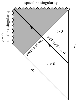
Figure 1: Penrose diagram of the BTZ black hole formed by the gravitational collapse of a null dust shell. The spacetime for $v<0$ corresponds to $\text{AdS}_{3}$ with a timelike singularity located at $r=0$. The surface $\Sigma$ is an initial Cauchy surface.

From the two-dimensional point of view, the metric (1) is obtained from the two-dimensional Jackiw-Teitelboim gravity ref:Liouville ,

$$S=\int dvdr~{}\sqrt{-g}~{}e^{\psi}(R-2\Lambda)~{},$$ (6)

where $g_{\mu\nu}$ and $R$ are the two-dimensional metric and the scalar curvature, respectively. For the solution (1), the field $\psi$ is given by $e^{\psi}=r$ and is continuous across the null dust shell.

II.2 Model field

We consider the evolution of a massless test scalar field $\phi$ which is minimally coupled to the Jackiw-Teitelboim gravity:

$$S=\int dvdr~{}\sqrt{-g}~{}\left[~{}e^{\psi}(R-2\Lambda)-\frac{1}{2}\,(\nabla\phi)^{2}~{}\right]~{}.$$ (7)

Its field equation becomes

$$(-\partial_{t}^{2}+\partial_{r_{*}}^{2})\phi=0,$$ (8)

where $t:=v-r_{*}$ and

$$r_{*}:=\int\frac{dr}{f(r)}=\begin{cases}\dfrac{1}{2\kappa}\,\ln\dfrac{r-r_{0}}{r+r_{0}}&\text{~{}~{}~{}for~{}~{}}v\geq 0\\ \\ \tan^{-1}(r)&\text{~{}~{}~{}for~{}~{}}v<0\end{cases}~{}.$$ (9)

Note that $v$ and $r$ are global coordinates, but $r_{*}$ and $t$ are local ones. In order to distinguish between the local coordinates in the region $v\geq 0$ and those in the region $v<0$, we often use the superscript ⁺ (^-) representing the local coordinates in the region $v\geq 0$ ($v<0$). Then, the retarded coordinates $u^{+}:=t^{+}-r_{*}^{+}$ and $u^{-}:=t^{-}-r_{*}^{-}$ are related to each other on the surface $v=0$ as

$$e^{-\kappa u^{+}}=\left|\,\frac{\tan(u^{-}/2)+r_{0}}{\tan(u^{-}/2)-r_{0}}\,\right| (-\pi<u^{-}\leq 0)~{}.$$ (10)

Let us remove a single spatial point $r=0$ from the spacetime to make an artificial model of a timelike singularity; this model can be fully analyzed (see Fig. 1). Since we remove the single spatial point $r=0$, we should specify a boundary condition for the scalar field there. To quantize the scalar field, the conserved Klein-Gordon (KG) inner product is necessary, so we require that the KG inner product is conserved. From the equation of motion of the scalar field, the variation of the inner product is given by

$$(\phi,\,\psi)_{\Sigma_{1}}-(\phi,\,\psi)_{\Sigma_{0}} =i\int^{\Sigma_{1}\cap(r=\infty)}_{\Sigma_{0}\cap(r=\infty)}d\Sigma^{\mu}~{}\big{(}\phi^{*}\nabla_{\mu}\psi-\psi\nabla_{\mu}\phi^{*}\big{)}\big{|}_{r=\infty}$$

$$-i\int^{\Sigma_{1}\cap(r=0)}_{\Sigma_{0}\cap(r=0)}d\Sigma^{\mu}~{}\big{(}\phi^{*}\nabla_{\mu}\psi-\psi\nabla_{\mu}\phi^{*}\big{)}\big{|}_{r=0}~{},$$ (11)

where $\Sigma_{0}$ and $\Sigma_{1}$ are spacelike surfaces.

We impose the Dirichlet boundary condition $\phi(r=\infty)=0$ at null infinity to mimic the fall-off condition of the scalar field in higher-dimensional asymptotically AdS spacetime. Then, the solution is represented by two arbitrary functions, $A^{+}$ and $A^{-}$ as

$$\phi(t,r_{*})=\begin{cases}A^{+}(u^{+})-A^{+}(v)&\text{~{}~{}~{}for~{}~{}}v\geq 0\\ A^{-}(u^{-})-A^{-}(v-\pi)&\text{~{}~{}~{}for~{}~{}}v<0\end{cases}~{}.$$ (12)

Then, for any fields $\phi$ and $\psi$ satisfying Eq. (8), the conservation of the KG inner product implies

$$0=\big{(}\phi^{*}\,\partial_{r_{*}}\psi-\psi\,\partial_{r_{*}}\phi^{*}\big{)}\big{|}_{r=0}~{}.$$ (13)

This condition is equivalent to

$$\left.\frac{\partial_{r_{*}}\phi}{\phi}\right|_{r=0}=c~{},$$ (14)

where $c$ is a real number which is common to all $\phi$. Thus, we have a model of scalar field whose evolution is characterized by the parameter $c$ via the boundary condition at the timelike singularity. The conditions $c=0$ and $c=\infty$ correspond to Neumann and Dirichlet boundary conditions, respectively.

This spacetime also has a usual spacelike singularity due to the gravitational collapse (see Fig. 1), but we do not address the issue how the information of the spacelike singularity is encoded in the correlators.

We choose the initial Cauchy surface $\Sigma$ so that it intersects with the horizon. This condition is necessary in order for the timelike singularity not to be visible to the asymptotic observer. If one chooses a null surface as $\Sigma$, this requirement is always met by placing $\Sigma$ arbitrarily close to the $v=0$ surface.

Under the WKB approximation LMR00 ; excursion , a two-point correlator has been obtained by calculating the geodesic distance between two points. This approximation is based on particle picture propagating along the geodesics. In our case, the particle corresponds to a massless particle propagating along the null geodesics between two points. In field theory picture, the parameter represents how the “wave packet” $\phi$ is reflected on the boundary, namely, it determines the phase shift. But in particle picture, it is not clear how the parameter $c$ appears in the two-point correlator. In the next section, we explicitly calculate a two-point correlator with two operators inserted on the timelike boundary at null infinity without using WKB formula.

III Construction of the bulk Wightman function

Our aim is to see if the information of the singularity appears in the two-point correlator by explicitly constructing the Wightman function. The Wightman function is defined by

$$W_{\Psi}(x_{1},x_{2}\,;c):=\left\langle\,\Psi\,;c\,\right|\,\phi(x_{1})\,\phi(x_{2})\,\left|\,\Psi\,;c\,\right\rangle~{},$$ (15)

where $x_{1}$ and $x_{2}$ are two spacetime points and $\left|\,\Psi\,;c\,\right\rangle$ is an initial quantum state on $\Sigma$ with boundary condition specified by $c$. There are many choices for the initial state $\left|\,\Psi\,;c\,\right\rangle$, so we need to see the $c$-dependence for all possible states to extract the information of the singularity. This state dependence is discussed in Sec. V. In this section, we pay attention to a vacuum state as the initial state.

III.1 Mode function

First, we explicitly construct the mode solution which satisfies the Dirichlet condition at null infinity and Eq. (14) at the origin in the $v<0$ region. Then, we extend the mode solution into the $v\geq 0$ region by the continuity condition across the $v=0$ null surface.

In the AdS region $v<0$, a positive frequency mode $f_{n}$ is given by

$$f_{n}(t,r_{*}) =\sqrt{\frac{2}{\pi\omega_{n}-\sin\pi\omega_{n}}}~{}e^{-i\omega_{n}t^{-}}\sin\big{[}~{}\omega_{n}(r_{*}^{-}-\pi/2)~{}\big{]}~{}.$$ (16)

The mode solution is a normalized solution of the form (12) satisfying the boundary condition (14). The KG inner product is used for normalization. The frequencies $\omega_{n}$ must satisfy the eigenvalue equation

$$0=\omega_{n}+c\,\tan\left(\frac{\pi\omega_{n}}{2}\right) (\omega_{n}>0)~{}.$$ (17)

The frequencies $\omega_{n}$ are ordered such that $\omega_{n}>\omega_{m}$ for $n>m$. Comparison of Eq. (16) with Eq. (12) leads to

$$A^{-}(u^{-}) =\frac{e^{-i\omega_{n}(u^{-}+\pi/2)}}{i\,\sqrt{2(\pi\omega_{n}-\sin\pi\omega_{n})}}~{}.$$ (18)

From the continuity of the mode function, one can extend the mode function $f_{n}$ obtained in the $v<0$ region into the $v\geq 0$ region. The continuity condition on the null surface $v=0$ becomes

$$A^{+}(u^{+})-A^{+}(0)=A^{-}(u^{-})-A^{-}(-\pi)~{}.$$ (19)

The above equation (19) implies

$$A^{+}(u^{+})=A^{-}\big{(}u^{-}(u^{+})\big{)}=\frac{\exp\left[-i\omega_{n}\big{\{}~{}u^{-}(u^{+})+\pi/2~{}\big{\}}\,\right]}{i\,\sqrt{2(\pi\omega_{n}-\sin\pi\omega_{n})}}~{},$$ (20)

where we use the relation $u^{+}|_{u^{-}=-\pi}=0$ obtained from Eq. (10).

We are especially concerned with the behavior of the Wightman function outside the horizon. Outside the horizon, the function $u^{-}(u^{+})$ is given by

$$u^{-}(u^{+})=-2~{}\tan^{-1}\left(r_{0}\,\frac{1+e^{-\kappa u^{+}}}{1-e^{-\kappa u^{+}}}\right)=:-2\,h(u^{+})~{},$$ (21)

and $\tan^{-1}(r_{0})<h(u^{+})<\pi/2$. Thus, the mode function in the $v\geq 0$ region is written as

$$f_{n}(t,r_{*}) =\frac{e^{-i\pi\omega_{n}/2}}{i\,\sqrt{2(\pi\omega_{n}-\sin\pi\omega_{n})}}~{}\left(e^{2i\omega_{n}h(u^{+})}-e^{2i\omega_{n}h(v)}\right)~{}.$$ (22)

III.2 Wightman function

One can expand the scalar field $\phi(x)$ by the mode function $f_{n}$ as

$$\phi(x)=\sum_{n=1}^{\infty}~{}\left(a_{n}\,f_{n}(x)+a_{n}^{\dagger}\,f_{n}^{*}(x)\right),$$ (23)

where $a_{n}$ and $a_{n}^{\dagger}$ are the annihilation and creation operators, respectively. Then, $a_{n}|0;c>=0$ defines the vacuum state associated with $f_{n}$ which satisfies the boundary condition (14).

The Wightman function for the vacuum state is given by

$$W_{0}(x_{1}\,;x_{2}\,;c)=\left\langle\,0\,;c\,\right|\,\phi(x_{1})\,\phi(x_{2})\,\left|\,0\,;c\,\right\rangle~{}.$$ (24)

In the black hole region $v,\,v^{\prime}>0$, the Wightman function is written by

$$W_{0}(u^{+}_{1},v_{1}\,;u^{+}_{2},v_{2}\,;c) =\mathcal{W}\big{(}\,h(u^{+}_{1})-h(u^{+}_{2})\,\big{)}-\mathcal{W}\big{(}\,h(u^{+}_{1})-h(v_{2})\,\big{)}$$

$$-\mathcal{W}\big{(}\,h(v_{1})-h(u^{+}_{2})\,\big{)}+\mathcal{W}\big{(}\,h(v_{1})-h(v_{2})\,\big{)}~{},$$ (25)

where

$$\mathcal{W}(\alpha):=\frac{1}{2}\,\sum_{n=1}^{\infty}~{}\frac{e^{2i\omega_{n}\,\alpha}}{\pi\omega_{n}-\sin(\pi\omega_{n})} (|\alpha|<\pi/2)~{}.$$ (26)

As a check, Eq. (25) consists of two contributions (terms with plus sign and those with minus sign). This is characteristic to the Dirichlet boundary condition at $u^{+}=v$. (Recall the method of images in electrostatics.)

The infinite sum in Eq. (26) can be written in terms of an integration (See Appendix A):

$$\mathcal{W}(\alpha) =\frac{c}{2\pi}\,\int^{\infty}_{0}\frac{dy}{y}~{}\frac{\cosh(2\alpha y)-1}{y\big{(}1+\cosh(\pi y)\big{)}+c\sinh(\pi y)}+\frac{1}{4\pi}\,\ln\left|\,\cot\alpha\,\right|$$

$$-\frac{i}{2}\,\frac{c}{2+\pi c}\,\alpha+\frac{i}{8}\,\text{sgn}(\alpha)~{}.$$ (27)

Therefore, the bulk Wightman function is

$$W_{0}(u^{+}_{1},v_{1}\,;u^{+}_{2},v_{2}\,;c)=\frac{c}{2\pi}\,\int^{\infty}_{0}\frac{dy}{y}~{}\frac{Q(y\,;u^{+}_{1},v_{1}\,;u^{+}_{2},v_{2}\,;c)}{y\,\big{(}1+\cosh(\pi y)\big{)}+c\sinh(\pi y)}$$

$$+\frac{1}{4\pi}\,\ln\left|\,\frac{\cot\big{[}\,\Delta(u^{+}_{1},u^{+}_{2})\,\big{]}\cdot\cot\big{[}\,\Delta(v_{1},v_{2})\,\big{]}}{\cot\big{[}\,\Delta(u^{+}_{1},v_{2})\,\big{]}\cdot\cot\big{[}\,\Delta(v_{1},u^{+}_{2})\,\big{]}}\,\right|+\frac{i}{8}\,\Big{(}\text{sgn}\big{[}\,\Delta(u^{+}_{1},u^{+}_{2})\,\big{]}$$

$$\hskip 56.9055pt+\text{sgn}\big{[}\,\Delta(v_{1},v_{2})\,\big{]}-\text{sgn}\big{[}\,\Delta(u^{+}_{1},v_{2})\,\big{]}-\text{sgn}\big{[}\,\Delta(v_{1},u^{+}_{2})\,\big{]}\Big{)}~{},$$ (28)

where $\Delta(s_{1},s_{2}):=h(s_{1})-h(s_{2})$ and

$$Q(y\,;u^{+}_{1},v_{1}\,;u^{+}_{2},v_{2}\,;c):=\cosh\big{[}\,2\Delta(u^{+}_{1},u^{+}_{2})\,y\,\big{]}+\cosh\big{[}\,2\Delta(v_{1},v_{2})\,y\,\big{]}$$

$$\hskip 113.81102pt-\cosh\big{[}\,2\Delta(u^{+}_{1},v_{2})\,y\,\big{]}-\cosh\big{[}\,2\Delta(v_{1},u^{+}_{2})\,y\,\big{]}$$

$$= -4\sinh\big{[}\,\Delta(u^{+}_{1},v_{1})\,y\,\big{]}\sinh\big{[}\,\Delta(u^{+}_{2},v_{2})\,y\,\big{]}$$

$$\hskip 85.35826pt\times\cosh\Big{[}\big{(}\,\Delta(u^{+}_{1},v_{2})+\Delta(v_{1},u^{+}_{2})\,\big{)}\,y\,\Big{]}~{}.$$ (29)

Note that the Wightman function outside the horizon (28) depends on $c$ only through the real part and that the imaginary part, which is the expectation value of commutator of the scalar field, is independent of $c$. Related issues are discussed in the next section.

It is instructive to see the behavior of the function  (25) near the infinity $r_{1}\rightarrow\infty$ and at the late time $t_{1}\rightarrow\infty$:

$$W_{0}(u^{+}_{1},v_{1}\,;u^{+}_{2},v_{2}\,;c)$$

$$\sim \frac{2}{r_{1}}\,h^{\prime}(t^{+}_{1})~{}\left[~{}\mathcal{W}\big{(}\,h(t^{+}_{1})-h(u^{+}_{2})\,\big{)}-\mathcal{W}\big{(}\,h(t^{+}_{1})-h(v_{2})\,\big{)}~{}\right]$$

$$\sim -\frac{4\kappa r_{0}}{1+r_{0}^{2}}\,\frac{e^{-\kappa t^{+}_{1}}}{r_{1}}\,\left[~{}\mathcal{W}\big{(}\,\tan^{-1}(r_{0})-h(u^{+}_{2})\,\big{)}-\mathcal{W}\big{(}\,\tan^{-1}(r_{0})-h(v_{2})\,\big{)}~{}\right]~{}$$ (30)

under the approximation

$$u^{+}=t^{+}-r^{+}_{*}\sim t^{+}+\frac{1}{r}~{}, v=t^{+}+r^{+}_{*}\sim t^{+}-\frac{1}{r}~{}.$$ (31)

In the third equation, the large $u^{+}$ expansion for $h(u^{+})$ is used [See Eq. (21)]:

$$h(u^{+})=\tan^{-1}(r_{0})+\frac{2r_{0}}{1+r_{0}^{2}}\,e^{-\kappa u^{+}}+O\big{(}e^{-2\kappa u^{+}}\big{)}~{}.$$ (32)

The scalar field decays exponentially, so the field loses the late-time correlation; this is due to the redshift factor and is common to black hole spacetimes. The quantum fields in a black hole background is expected to become a thermal state at temperature $T_{\rm BH}=\kappa/(2\pi)$ due to the Hawking radiation and that the time scale of its thermalization is the order of magnitude of $O(1/T_{\rm BH})$. The form of Eq. (30) is consistent with the expectation.

IV Boundary Wightman function

According to the standard AdS/CFT procedure BDHM ; Kle-Wit , the boundary Wightman function $G_{\Psi}(t^{+}_{1},t^{+}_{2}\,;c)$ is obtained by

$$G_{\Psi}(t^{+}_{1},t^{+}_{2}\,;c)=\lim_{r_{1},r_{2}\rightarrow\infty}~{}r_{1}\,r_{2}~{}W_{\Psi}(t^{+}_{1},r_{1}\,;t^{+}_{2},r_{2}\,;c)~{}.$$ (33)

Then, the Wightman function $W_{0}$ behaves near the infinity as

$$W_{0}(u^{+}_{1},v_{1}\,;u^{+}_{2},v_{2}\,;c)\sim-\frac{4\,h^{\prime}(t^{+}_{1})\,h^{\prime}(t^{+}_{2})}{r_{1}\,r_{2}}~{}\mathcal{W}^{\prime\prime}\big{[}\Delta(t^{+}_{1},t^{+}_{2})\big{]}~{}.$$ (34)

Thus, the boundary Wightman function $G_{0}(t^{+}_{1},t^{+}_{2}\,;c)$ for the vacuum becomes

$$G_{0}(t^{+}_{1},t^{+}_{2}\,;c) =-\frac{4\,h^{\prime}(t^{+}_{1})\,h^{\prime}(t^{+}_{2})}{\pi}~{}\left(~{}2c\,\int^{\infty}_{0}dy~{}\frac{y\,\cosh\big{[}~{}2\Delta(t^{+}_{1},t^{+}_{2})\,y~{}\big{]}}{y\big{(}1+\cosh(\pi y)\big{)}+c\sinh(\pi y)}\right.$$

$$\left.\hskip 85.35826pt+\frac{\cos\big{[}2\Delta(t^{+}_{1},t^{+}_{2})\big{]}}{\sin^{2}\big{[}2\Delta(t^{+}_{1},t^{+}_{2})\big{]}}+\frac{i\pi}{4}\,\delta^{\prime}\big{[}\,\Delta(t^{+}_{1},t^{+}_{2})\,\big{]}~{}\right)~{}.$$ (35)

The imaginary part is independent of $c$, which reflects the state-independence of the imaginary part of the bulk Wightman function.

Let us see some specific examples. For $c=0$ and $c=\infty$, the boundary Wightman function $G_{0}(t^{+}_{1},t^{+}_{2}\,;c)$ can be written in analytic form:

$$\text{Re}\left[~{}G_{0}(t^{+}_{1},t^{+}_{2}\,;c=0)~{}\right]=-\frac{4\,h^{\prime}(t^{+}_{1})\,h^{\prime}(t^{+}_{2})}{\pi}~{}\frac{\cos\big{[}2\Delta(t^{+}_{1},t^{+}_{2})\big{]}}{\sin^{2}\big{[}2\Delta(t^{+}_{1},t^{+}_{2})\big{]}}~{},$$ (36)

$$\text{Re}\left[~{}G_{0}(t^{+}_{1},t^{+}_{2}\,;c=\infty)~{}\right]=-\frac{4\,h^{\prime}(t^{+}_{1})\,h^{\prime}(t^{+}_{2})}{\pi}~{}\frac{1}{\sin^{2}\big{[}2\Delta(t^{+}_{1},t^{+}_{2})\big{]}}~{}.$$ (37)

We also plot the real part of $G_{0}$ in Fig. 2 for several values of $c$.

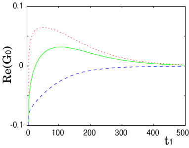
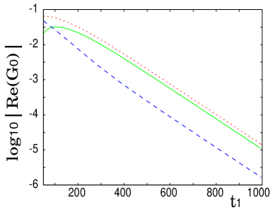
Figure 2: (color online) The real part of the two-point function $G_{0}(t_{1},10^{-5}\,;\,c)$. The dotted, solid, and dashed lines correspond to $c=1$, $c=10$, and $c=100$, respectively.

As is clear from Eq. (35), the information behind the horizon (the boundary condition set behind the horizon) is imprinted on the boundary Wightman function in the outer communicating region. This fact is not due to the causality violation but due to the entanglement between two states inside and outside the horizon on the initial Cauchy surface $\Sigma$. So, it is generic to the models with the timelike singularity such as ours. To see this, let us consider the evolution of the Wightman function for general black hole spacetime.

From the field equation of $\phi$, the Wightman function for a linear scalar field in the outer communicating region evolves as

$$W_{\Psi}(x_{1}\,;x_{2}\,;c)$$

$$= \int_{\Sigma}d\Sigma^{\mu}_{y_{1}}\,\int_{\Sigma}d\Sigma^{\nu}_{y_{2}}~{}G_{R}(x_{1}\,;y_{1})\,G_{R}(x_{2}\,;y_{2})\stackrel{{\scriptstyle\leftrightarrow}}{{\nabla}}{}^{y_{1}}_{\mu}\stackrel{{\scriptstyle\leftrightarrow}}{{\nabla}}{}^{y_{2}}_{\nu}~{}W_{\Psi}(y_{1}\,;y_{2}\,;c)~{},$$ (38)

where $x_{1}$ and $x_{2}$ are in the outer communicating region and $\Sigma$ is an initial Cauchy surface. The function $G_{R}(x;y)$ is the retarded Green function of the equation of motion for the scalar field, so it is causal and independent of a quantum state. So, it is independent of $c$ in the outer-communicating region. Therefore, the $c$-dependence on the Wightman function could come only from the initial Cauchy surface $\Sigma$ in the outer communicating region, and it indeed comes as follows.

Since the event horizon is just a null surface dividing the spacetime into two regions, it is unnatural to set the quantum state $\Psi$ by a product of states inside and outside the horizon. Physical quantities constructed from the energy-momentum tensor could diverge on the horizon. So, the initial state in the outer communicating region could be entangled with the one behind the horizon. This implies that the information about the boundary condition is imprinted on the boundary Wightman function through the entanglement on $\Sigma$ for general $\Psi$.

The initial value of the bulk Wightman function depends not only on the boundary condition $c$, but also on the choice of the quantum states. Therefore, the detectability of the information behind the horizon is a delicate problem, though the information behind the horizon is imprinted on the boundary Wightman function in principle.

V Wightman function for squeezed states

In this section, we discuss whether we can derive the information about parameter $c$ from $G_{\Psi}(t^{+}_{1},t^{+}_{2}\,;c)$ when the initial state is not restricted to the vacuum state. The reason why such a consideration is necessary is because the asymptotic observer has no way to determine the initial state uniquely; the observer can have access to only part of the Cauchy surface. In general, it seems a difficult task to derive the information without fixing the initial state because $G_{\Psi}(t^{+}_{1},t^{+}_{2}\,;c)$ depends also on the initial quantum state $\left|\,\Psi\,;c\,\right\rangle$.

In order to distinguish between two boundary conditions $c$ and $c^{\prime}$ from the behavior of the boundary Wightman functions, the following inequality should hold for any $\Psi$ and $\Psi^{\prime}$:

$$G_{\Psi}(t^{+}_{1},t^{+}_{2}\,;c) =\lim_{r_{1},r_{2}\rightarrow\infty}~{}r_{1}\,r_{2}~{}\left\langle\,\Psi\,;c\,\right|\,\phi(x_{1})\,\phi(x_{2})\,\left|\,\Psi\,;c\,\right\rangle$$

$$\neq\lim_{r_{1},r_{2}\rightarrow\infty}~{}r_{1}\,r_{2}~{}\left\langle\,\Psi^{\prime}\,;c^{\prime}\,\right|\,\phi(x_{1})\,\phi(x_{2})\,\left|\,\Psi^{\prime}\,;c^{\prime}\,\right\rangle=G_{\Psi^{\prime}}(t^{+}_{1},t^{+}_{2}\,;c^{\prime})~{}.$$ (39)

Otherwise, the boundary Wightman function is degenerate for the boundary conditions. If the function is degenerate, it is impossible to detect the information unless we can perfectly control the initial state.

Unfortunately, it is impossible to argue the behavior of $G_{\Psi}$ for general initial states $\Psi$. Thus, we discuss the behavior of $G_{\Psi}$ for a restricted class of initial states, which is a class of squeezed states. The squeezed state $\left|\,\bar{0}\,;c\,\right\rangle$ is defined by $\bar{a}_{n}\left|\,\bar{0}\,;c\,\right\rangle=0$ for any $\bar{a}_{n}$, where the new annihilation operators $\bar{a}_{n}$ are given by the Bogoliubov transformation

$$\bar{a}_{n}=\sum^{\infty}_{n^{\prime}=1}\left(\alpha^{*}_{nn^{\prime}}\,a_{n^{\prime}}-\beta^{*}_{nn^{\prime}}\,a_{n^{\prime}}^{\dagger}\right)~{},$$ (40)

which corresponds to the transformation of the mode functions

$$\bar{f}_{n}(x)=\sum^{\infty}_{n^{\prime}=1}\big{(}~{}\alpha_{nn^{\prime}}\,f_{n^{\prime}}(x)+\beta_{nn^{\prime}}\,f^{*}_{n^{\prime}}(x)~{}\big{)}~{}.$$ (41)

The Bogoliubov coefficients $\alpha_{nn^{\prime}}$ and $\beta_{nn^{\prime}}$ should satisfy the unitarity condition

$$\begin{cases}{}~{}\displaystyle{\delta_{nn^{\prime}}=\sum^{\infty}_{m=1}\left(\alpha_{nm}\,\alpha^{*}_{mn^{\prime}}-\beta_{nm}\,\beta^{*}_{mn^{\prime}}\right)}\\ {}~{}\displaystyle{0=\sum^{\infty}_{m=1}\left(\alpha_{nm}\,\beta_{mn^{\prime}}-\beta_{nm}\,\alpha_{mn^{\prime}}\right)}\end{cases}~{}.$$ (42)

Using this unitarity condition, we can relate the Wightman function $W_{\bar{0}}$ for the squeezed state to $W_{0}$ for the vacuum:

$$W_{\bar{0}}(x_{1}\,;x_{2}\,;c) :=\left\langle\,\bar{0}\,;c\,\right|\,\phi(x_{1})\,\phi(x_{2})\,\left|\,\bar{0}\,;c\,\right\rangle$$

$$=W_{0}(x_{1}\,;x_{2}\,;c)+2\sum_{n,n^{\prime}=1}^{\infty}~{}\text{Re}\left[~{}f_{n}(x_{1})\,\beta^{*}_{n^{\prime}n}\,\bar{f}_{n^{\prime}}(x_{2})~{}\right]~{}.$$ (43)

Then, we have

$$G_{\bar{0}}(t^{+}_{1},t^{+}_{2}\,;c)-G_{0}(t^{+}_{1},t^{+}_{2}\,;c)=4\,h^{\prime}(t^{+}_{1})\,h^{\prime}(t^{+}_{2})~{}\sum_{n,n^{\prime}=1}^{\infty}~{}\frac{4\,\omega_{n}\,\omega_{n^{\prime}}}{\sqrt{(\pi\omega_{n}-\sin\pi\omega_{n})(\pi\omega_{n^{\prime}}-\sin\pi\omega_{n^{\prime}})}}$$

$$\times\text{Re}\left[~{}\left(\sum_{m=1}^{\infty}\beta^{*}_{mn}\,\beta_{mn^{\prime}}\right)e^{-i\pi(\omega_{n}-\omega_{n^{\prime}})/2}~{}e^{2i\left\{\omega_{n}h(t^{+}_{1})-\omega_{n^{\prime}}h(t^{+}_{2})\right\}}\right.$$

$$\hskip 56.9055pt\left.+\left(\sum_{m=1}^{\infty}\beta^{*}_{mn}\,\alpha_{mn^{\prime}}\right)e^{-i\pi(\omega_{n}+\omega_{n^{\prime}})/2}~{}e^{2i\left\{\omega_{n}h(t^{+}_{1})+\omega_{n^{\prime}}h(t^{+}_{2})\right\}}~{}\right]~{}.$$ (44)

For simplicity, consider the case where the Bogoliubov coefficients are diagonal, $\left|\,\alpha_{nn^{\prime}}\,\right|=\delta_{nn^{\prime}}\,\cosh\chi_{n}$ and $\left|\,\beta_{nn^{\prime}}\,\right|=\delta_{nn^{\prime}}\,\sinh\chi_{n}$. Then, the difference of the boundary Wightman functions between the squeezed state and the vacuum state is given by

$$G_{\bar{0}}(t^{+}_{1},t^{+}_{2}\,;c)-G_{0}(t^{+}_{1},t^{+}_{2}\,;c)=4\,h^{\prime}(t^{+}_{1})\,h^{\prime}(t^{+}_{2})~{}\sum_{n=1}^{\infty}~{}\frac{2\,\omega_{n}^{2}\,\sinh(2\chi_{n})}{\pi\omega_{n}-\sin\pi\omega_{n}}$$

$$\times\Big{(}\tanh\chi_{n}\cos\left[~{}2\omega_{n}\,\Delta(t^{+}_{1},t^{+}_{2})~{}\right]+\cos\left[~{}2\omega_{n}\left(H(t^{+}_{1},t^{+}_{2})-\pi/2\right)+\theta_{n}~{}\right]\Big{)}~{},$$ (45)

where $H(s_{1},s_{2}):=h(s_{1})+h(s_{2})$ and $\theta_{n}:=\text{arg}(\alpha_{nn})-\text{arg}(\beta_{nn})$. On the other hand, from Eq. (35), we have

$$G_{0}(t^{+}_{1},t^{+}_{2}\,;c^{\prime})-G_{0}(t^{+}_{1},t^{+}_{2}\,;c)=-(c^{\prime}-c)\,\frac{2\,h^{\prime}(t^{+}_{1})\,h^{\prime}(t^{+}_{2})}{\pi}~{}$$

$$\times\int_{-\infty}^{\infty}dy~{}\frac{e^{2\Delta(t^{+}_{1},t^{+}_{2})\,y}}{\cosh^{2}(\pi y/2)}\,\frac{y^{2}}{\big{[}y+c\tanh(\pi y/2)\big{]}\big{[}y+c^{\prime}\tanh(\pi y/2)\big{]}}~{}.$$ (46)

The difference between the Wightman functions for the vacuum states satisfying different boundary conditions essentially depends only on $\Delta(t^{+}_{1},t^{+}_{2})=h(t^{+}_{1})-h(t^{+}_{2})$, not on $H(t^{+}_{1},t^{+}_{2})$. So, if the Wightman function of the vacuum state characterized by $c$ is represented by the function of a squeezed state characterized by another parameter $c^{\prime}$, the $H(t^{+}_{1},t^{+}_{2})$ dependence in Eq. (45) should disappear for the range $2\tan^{-1}(r_{0})<H(t^{+}_{1},t^{+}_{2})<\pi$. [Note that $\tan^{-1}(r_{0})<h(t^{+})<\pi/2$. See the sentence immediately after Eq. (21).]

For simplicity, let us examine the $c^{\prime}=0$ case. Substituting $\omega_{n}=2n-1$ into Eq. (45), the terms with $H(t^{+}_{1},t^{+}_{2})$ reduce to

$$f(H):=\frac{8h^{\prime}(t^{+}_{1})h^{\prime}(t^{+}_{2})}{\pi}\sum_{n=1}^{\infty}(2n-1)\sinh(2\chi_{n})\cos[2(2n-1)(H-\pi/2)+\theta_{n}].$$ (47)

This function is anti-periodic with period $\pi/2$, i.e., $f(H+\pi/2)=-f(H)$, so the function $f$ has to vanish for the range $2\tan^{-1}(r_{0})<H(t^{+}_{1},t^{+}_{2})<\pi$ for $r_{0}<1$. This is improbable unless all $\chi_{n}$ are zero. Thus, the Wightman function for the vacuum state at nonzero $c$ cannot be represented by the function for any squeezed state at $c=0$.

Unfortunately, it is impossible to show Eq. (39) rigorously for general $\Psi$. But the above argument may suggest that it is possible to obtain the information about $c$ even when the initial state is unknown.

We have noted thermalization behavior in Eq. (30). Similar to the discussion there, the appearance of $h^{\prime}(t^{+}_{1})$ in Eqs. (44) and (46) suggests that the (boundary) Wightman function “forgets” its initial data and boundary condition at late time and it settles into a unique thermal state. Namely, this factor has the expected form from the Hawking radiation. The differences left are the minor ones (for instance, just the overall factor due to the difference in the boundary condition $c$ and so on.)

VI Conclusion and discussion

We have investigated how information about the singularity inside the BTZ black hole formed by gravitational collapse is restored from the boundary correlator. A model of timelike singularity is artificially constructed to represent the information as one-parameter family of boundary conditions. When initial quantum state is restricted to a vacuum state, the parameter $c$ is restored from the asymptotic behavior of the correlator. When it is not restricted, it is not clear whether we can derive the information since we cannot observe the whole initial data. If the correlator is degenerate on the boundary of spacetime, we cannot derive the information. In the previous section, we show that the boundary correlator is not degenerate for a particular class of excited states. This may imply that one can still derive the information about singularity inside an AdS black hole via boundary correlators. But we are not able to study the issue for generic excited states, so the result is not conclusive.

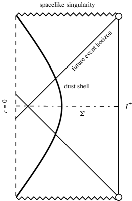
Figure 3: Penrose diagram of the time-symmetric spacetime with a collapsing dust shell

Let us consider the above issue in the framework of the finite temperature AdS/CFT correspondence. Originally, the AdS/CFT correspondence is defined in Euclidean signature, but one may analytically continue it in Lorentzian signature. In this case, a vacuum state is naturally selected by the analytic continuation. Thus, the Euclidean prescription of AdS/CFT can restrict initial quantum states in Lorentzian signature. By such a restriction, it may be possible to derive the information about singularity inside an AdS black hole although the prescription does not pick up a unique initial state. The AdS/CFT correspondence is special in this sense and probably it is in this sense that the boundary theory can encode information behind the horizon.

The analytic continuation is also possible for an AdS black hole formation if one uses a time-symmetric AdS black hole. (The analytic continuation must be performed on the time-symmetric Cauchy surface as seen in the maximally extended AdS-Schwarzschild spacetime Gibbons:1990ns .) Figure 3 shows the Penrose diagram of an AdS black hole formed by the gravitational collapse of a dust shell. Again one would place the timelike singularity parametrized by $c$ at $r=0$ in the spacetime. The parameter $c$ would appear in the asymptotic behavior of the boundary correlators and one could extract the information since the allowed initial quantum state on $\Sigma^{\prime}$ is restricted. Note that this timelike singularity is part of the Euclidean spacetime as well; From the Euclidean point of view, this is the reason why the information can be encoded in the boundary correlators. On the contrary, this spacetime also has a spacelike singularity, but the spacelike singularity is not part of the Euclidean spacetime. Thus, extracting the information of the spacelike singularity is a completely different issue; analyticity seems to play a key roleLMR00 ; KOS02 ; FHKS ; excursion ; FHMMRS05 .

Current knowledge of the AdS/CFT correspondence is not enough to completely resolve the singularity problem. In particular, we consider the $s$-wave sector in the BTZ black hole background, but the ${\rm AdS}_{2}/{\rm CFT}_{1}$ correspondence is probably least understood among the AdS/CFT in various dimensions. Some aspects are explored, e.g., in Refs. ads2 . Most references consider the near-horizon limit of the extreme four-dimensional Reissner-Nordström black hole, and one encounters various difficulties. We expect similar problems in our case as well if we seriously try to understand the correspondence in the ${\rm AdS}_{2}$ context since our spacetime is really asymptotically ${\rm AdS}_{3}$ in disguise. Probably the Jackiw-Teitelboim black hole is consistently understood only in the zero mass limit in the ${\rm AdS}_{2}/{\rm CFT}_{1}$ context. One obvious approach to overcome this problem is to go back to three dimensions and use the ${\rm AdS}_{3}/{\rm CFT}_{2}$ correspondence. For example, one may compute the correlators of a three-dimensional scalar field propagating on the BTZ black hole formed by the gravitational collapse. In this case, the correlator will involve an infinite sum due to the infinite number of images, so the expressions may be more complicated than the one here.

Moreover, the finite temperature AdS/CFT correspondence is not well-understood quantitatively compared with zero temperature one. Precise correspondence between the bulk and the boundary theories is not known. We do not pursue this issue in this paper but it is important. Strong coupling dynamics for finite temperature gauge theories is in general intractable. In order to overcome the difficulty, hydrodynamic description of gauge theory plasmas using the AdS/CFT correspondence may be useful since experiments and other tools (such as lattice calculations) are available there.

Appendix A Evaluation of Eq. (26)

In order to evaluate Eq. (26) in the black hole region, we introduce $p(\omega)$ as

$$p(\omega):=\omega\cos\frac{\pi\omega}{2}+c\sin\frac{\pi\omega}{2}.$$ (48)

By using the fact

$$\frac{1}{\pi\omega_{n}-\sin\pi\omega_{n}}=\frac{c}{2\omega_{n}\cos(\pi\omega_{n}/2)}\frac{1}{p^{\prime}(\omega_{n})},$$ (49)

one can replace the summation of Eq. (26) with the following contour integration in the complex $z$ plane (Fig. 4)):

$${\cal W}(\alpha) = \frac{c}{8\pi i}\oint_{C_{1}+C_{2}+C_{3}+C_{4}}\frac{e^{2i\alpha z}}{z\cos(\pi z/2)p(z)}dz$$ (50)

$$- \frac{c}{4}\sum_{n=0}^{\infty}\mbox{Res}\left[\frac{1}{\cos(\pi z/2)};z=2n+1\right]\frac{e^{2i\alpha z}}{z\,p(z)}\Biggl{|}_{z=2n+1}$$

$$= \frac{c}{8\pi i}\oint_{C_{1}+C_{2}+C_{3}+C_{4}}\frac{e^{2i\alpha z}}{z\cos(\pi z/2)p(z)}dz$$

$$+\frac{1}{4\pi}\ln\left|\cot\alpha\right|+\frac{i}{8}\mbox{sgn}(\alpha).$$

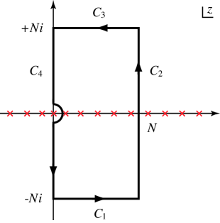
Figure 4: The contour of ${\cal W}$ in the complex $z$ plane. The number $N$ is an arbitrary large positive number with $N\neq 2n+1$.

Since $|\alpha|<\pi/2$, $C_{1}$, $C_{2}$, and $C_{3}$ contour integrations disappear in the large $N$ limit ($N\to\infty$). The integration along $C_{4}$ reduces to

$$\int_{C_{4}}\frac{dz}{8\pi i}\frac{e^{2i\alpha z}}{z\cos(\pi z/2)}\frac{1}{p(z)} = \text{P}\int^{\infty}_{-\infty}\frac{dy}{8\pi}\frac{e^{-2\alpha y}}{y\cosh(\pi y/2)[y\cosh(\pi y/2)+c\sinh(\pi y/2)]}$$

$$-\frac{1}{8}\,\text{Res}\left(\frac{e^{2i\alpha z}}{z\cos(\pi z/2)}\,\frac{1}{p(z)}\right)\Biggl{|}_{z=0}$$

$$= \frac{1}{2\pi}\int^{\infty}_{0}\frac{dy}{y}\frac{\cosh(2\alpha y)-1}{y(1+\cosh(\pi y))+c\sinh(\pi y)}-\frac{i\alpha}{2(2+\pi c)},$$

where we removed a singularity at $y=0$ by adding an $\alpha$-independent term; this does not affect the value of $W_{0}$.

References

- (1) J.M. Maldacena, “Eternal black holes in Anti-de-Sitter,” JHEP 0304 (2003) 021, [arXiv:hep-th/0106112].
- (2) J. Louko, D. Marolf, and S.F. Ross, “Geodesic propagators and black hole holography,” Phys. Rev. D62, 044041 (2000), [arXiv:hep-th/0002111].
- (3) P. Kraus, H. Ooguri, and S. Shenker, “Inside the horizon with AdS/CFT,” Phys. Rev. D67, 124022 (2003), [arXiv:hep-th/0212277].
- (4) L. Fidkowski, V. Hubeny, M. Kleban, and S. Shenker, “The black hole singularity in AdS/CFT,” JHEP 0402 (2004) 014, [arXiv:hep-th/0306170].
- (5) G. Festuccia and H. Liu, “Excursions beyond the horizon: Black hole singularities in Yang-Mills theories (I),” [arXiv:hep-th/0506202].
- (6) B. Freivogel, V. Hubeny, A. Maloney, R. C. Myers, M. Rangamani, and S. Shenker, “Inflation in AdS/CFT,” JHEP 0603 (2006) 007, [arXiv:hep-th/0510046].
- (7) J. Louko and D. Marolf, “Single-exterior black holes and the AdS-CFT conjecture,” Phys. Rev. D59, 066002 (1999), [arXiv:hep-th/9808081].
- (8) V. Balasubramanian and S.F. Ross, “Holographic particle detection,” Phys. Rev. D61, 044007 (2000), [arXiv:hep-th/9906226].
- (9) U.H. Danielsson, E. Keski-Vakkuri, and M. Kruczenski, “Black hole formation in AdS and thermalization on the boundary,” JHEP 0002 (2000) 039, [arXiv:hep-th/9912209].
- (10) M. Reed and B. Simon, Fourier Analysis, Self-Adjointness, (Academic Press, New York, 1975).
- (11) N.D. Birrell and P.C.W. Davies, Quantum field in curved spacetime, (Cambridge University Press, Cambridge, England, 1982).
- (12) V. Husain, “Radiation collapse and gravitational waves in three dimensions,” Phys. Rev. D50, 2361 (1994), [arXiv:gr-qc/9404047].
- (13) C. Teitelboim, “The Hamiltonian structure of two-dimensional space-time and its relation with the conformal anomaly” in Quantum theory of gravity, ed. S.M. Christensen, (Adam Hilger, Bristol, 1984) ; R. Jackiw, “Liouville field theory; A two-dimensional model for gravity?” ibid.
- (14) T. Banks, M.R. Douglas, G.T. Horowitz, and E.J. Martinec, “AdS dynamics from conformal field theory,” [arXiv:hep-th/9808016].
- (15) I.R. Klebanov and E. Witten, “AdS/CFT correspondence and symmetry breaking,” Nucl. Phys. B556, 89 (1999), [arXiv:hep-th/9905104].
- (16) G.T. Horowitz and J. Maldacena, “The black hole final state,” JHEP 0402 (2004) 008, [arXiv:hep-th/0310281].
- (17) G.W. Gibbons and J.B. Hartle, “Real tunneling geometries and the large scale topology of the universe,” Phys. Rev. D42, 2458 (1990).
- (18) A. Strominger, “AdS(2) quantum gravity and string theory,” JHEP 9901 (1999) 007, [arXiv:hep-th/9809027]; J.M. Maldacena, J. Michelson and A. Strominger, “Anti-de Sitter fragmentation,” JHEP 9902 (1999) 011, [arXiv:hep-th/9812073]; M. Spradlin and A. Strominger, “Vacuum states for AdS(2) black holes,” JHEP 9911 (1999) 021, [arXiv:hep-th/9904143];
- (19) P.K. Kovtun, D.T. Son and A.O. Starinets, “Viscosity in Strongly Interacting Quantum Field Theories from Black Hole Physics,” Phys. Rev. Lett. 94, 111601 (2005), [arXiv:hep-th/0405231].
- (20) J. Mas, “Shear viscosity from R-charged AdS black holes,” JHEP 0603 (2006) 016, [arXiv:hep-th/0601144] ; D.T. Son and A.O. Starinets, “Hydrodynamics of R-charged black holes,” JHEP 0603 (2006) 052, [arXiv:hep-th/0601157] ; O. Saremi, “The viscosity bound conjecture and hydrodynamics of M2-brane theory at finite chemical potential,” [arXiv:hep-th/0601159] ; K. Maeda, M. Natsuume and T. Okamura, “Viscosity of gauge theory plasma with a chemical potential from AdS/CFT correspondence,” Phys. Rev. D73, 066013 (2006), [arXiv:hep-th/0602010].