Particle Creation by a Moving Boundary with Robin Boundary Condition

Abstract

We consider a massless scalar field in 1+1 dimensions satisfying a Robin boundary condition (BC) at a non-relativistic moving boundary. We derive a Bogoliubov transformation between input and output bosonic field operators, which allows us to calculate the spectral distribution of created particles. The cases of Dirichlet and Neumann BC may be obtained from our result as limiting cases. These two limits yield the same spectrum, which turns out to be an upper bound for the spectra derived for Robin BC. We show that the particle emission effect can be considerably reduced (with respect to the Dirichlet/Neumann case) by selecting a particular value for the oscillation frequency of the boundary position.

1 Introduction

Moving bodies experience fundamental energy damping [1] [2] and decoherence [3] mechanisms due to the scattering of vacuum field fluctuations. The damping is accompanied by the emission of particles (photons in the case of the electromagnetic field) [4], thus conserving the total energy of the body-plus-field system [5][6]. This dynamical (or nonstationary) Casimir effect has been analyzed for a variety of three-dimensional geometries, including parallel plane plates [7], cylindrical waveguides [8], and rectangular [9], cylindrical [10] and spherical cavities [11]. It also depends on the details of the coupling between the field and the body, which can usually be cast in the form of boundary conditions (BC) for the field. Of particular theoretical relevance is the Robin BC, which continuously interpolates the Dirichlet and Neumann BC. For a massless scalar field in 1+1 dimensions, it reads

$$\frac{\partial\phi}{\partial x}(t,x_{0})=\frac{1}{\beta}\,\phi(t,x_{0}),$$ (1)

where $x_{0}$ is the position of the boundary. The positive parameter $\beta$ represents a time scale (we take $c=1$) associated to the time delay (or phase shift) characteristic of reflection at the Robin boundary [12], which can be interpreted in terms of a simple mechanical model [13]. According to eq. (1), Dirichlet and Neumann BC are obtained as the limiting cases $\beta\rightarrow 0$ and $\beta\rightarrow\infty,$ respectively.

We consider a semi-infinite slab (extending from $-\infty$ to $x=\delta q(t)$) following a prescribed nonrelativistic motion, with the Robin boundary at $\delta q(t).$ We have recently computed the dynamical Casimir force on the slab, which contains dissipative as well as dispersive components [12]. In this paper, we will analyze in detail the particle creation effect and compute the corresponding spectral distribution.

2 Input-Output Bogoliubov Transformation

In the instantaneously co-moving frame the massless scalar field satisfies

$$\frac{\partial\phi^{\prime}}{\partial x^{\prime}}|_{\rm bound}=\frac{1}{\beta}\,\phi^{\prime}|_{\rm bound},$$ (2)

Neglecting terms of the order of $[\delta{\dot{q}}(t)]^{2},$ we find, in the laboratory frame,

$$\left[\frac{\partial}{\partial x}+\delta{\dot{q}}(t)\frac{\partial}{\partial t}\right]\phi(t,\delta{q}(t))=\frac{1}{\beta}\,\phi(t,\delta{q}(t)).$$ (3)

We assume that final position coincides with initial one, which is taken at $x=0.$ Hence

$$\lim_{t\rightarrow\pm\infty}\delta q(t)=0.$$ (4)

Jointly with the nonrelativistic approximation, this condition implies that $\delta q(t)$ is much smaller than the wavelengths $\lambda$ of the created particles. In fact, we will show that the frequencies of the particles are bounded by the mechanical frequencies $\omega_{0}:$ $\omega=2\pi/\lambda\leq\omega_{0}.$ Since $\omega_{0}\delta q\sim\delta{\dot{q}}\ll 1,$ we have $\delta q(t)\ll\lambda.$

Thus, we may analyze eq.  (3) by expanding up to first order in $\delta q$ and its derivatives. This amounts to calculate the effect of the motion as a small perturbation [2]:

$$\phi(t,x)=\phi_{0}(t,x)+\delta\phi(t,x),$$ (5)

where the unperturbed field $\phi_{0}$ corresponds to a solution with a static boundary at $x=0.$ The first-order field $\delta\phi$ then satisfies the following BC at $x=0:$

$$\frac{\partial\delta\phi}{\partial x}(t,0)-\frac{1}{\beta}\delta\phi(t,0)=\delta q(t)\left[\frac{1}{\beta}\frac{\partial\phi_{0}}{\partial x}(t,0)-\frac{\partial^{2}\phi_{0}}{\partial x^{2}}(t,0)\right]-\delta\dot{q}(t)\frac{\partial\phi_{0}}{\partial t}(t,0)\,.$$ (6)

It is convenient to use the Fourier representation

$$\Phi(\omega,x)=\int dte^{i\omega t}\phi(t,x).$$

The unperturbed field satisfies the Robin BC at $x=0.$ Its normal mode expansion for $x>0$ is given by

$$\Phi_{0}(\omega,x)=N(\omega)[\sin(\omega x)+\omega\beta\cos(\omega x)]\left[\Theta(\omega)a(\omega)-\Theta(-\omega)a(-\omega)^{\dagger}\right],$$ (7)

with

$$N(\omega)=\sqrt{\frac{4\pi}{|\omega|(1+\beta^{2}\omega^{2})}}$$

and $\Theta(x)$ denoting Heaviside step function. The bosonic operators $a(\omega)$ and $a(\omega)^{\dagger}$ satisfy the commutation relation

$$[a(\omega),\,a(\omega^{\prime})^{\dagger}]=2\pi\,\delta(\omega-\omega^{\prime}).$$ (8)

To solve eq. (6) for $\delta\Phi(\omega,x)$ in terms of $\Phi_{0}(\omega,0)$ (with $x>0$), we use suitably defined Green functions, obeying the differential equation

$$\left(\frac{\partial^{2}}{\partial x^{2}}+\omega^{2}\right)G(\omega,x,x^{\prime})=\delta(x-x^{\prime}).$$ (9)

¿From Green’s theorem, we find

$$\delta\Phi(\omega,x^{\prime})=-\delta\Phi(\omega,0)\frac{\partial}{\partial x}G(\omega,0,x^{\prime})+G(\omega,0,x^{\prime})\frac{\partial}{\partial x}\delta\Phi(\omega,0).$$ (10)

This result is more easily combined with eq. (6) if we select a solution $G_{\rm R}(\omega,x,x^{\prime})$ of eq. (9) satisfying the Robin BC at $x=0.$ With this Robin Green function, we immediately obtain the first-order field from eq. (10) in terms of the BC satisfied by $\delta\Phi(\omega,x)$ as given by the Fourier transform of eq. (6). Then, the complete field is written as

$$\Phi(\omega,x)=\Phi_{0}(\omega,x)+G_{\rm R}(\omega,0,x)\left[\frac{\partial}{\partial x}\delta\Phi(\omega,0)-\frac{\delta\Phi(\omega,0)}{\beta}\right],$$ (11)

with

$$\frac{\partial}{\partial x}\delta\Phi(\omega,0)-\frac{\delta\Phi(\omega,0)}{\beta}=\frac{1}{\beta}\,\int\frac{d\omega^{\prime}}{2\pi}\left[\frac{\partial\Phi_{0}}{\partial x}(\omega,0)+\omega\omega^{\prime}\Phi_{0}(\omega,0)\right]\delta Q(\omega-\omega^{\prime}),$$ (12)

where $\delta Q(\omega)$ is the Fourier transform of $\delta q(t).$

If we replace $G_{\rm R}$ in eq. (11) by the retarded Robin Green function, given by

$$G_{\rm R}^{\rm ret}(\omega,0,x)=\frac{\beta}{1-i\beta\omega}e^{i\omega x},$$ (13)

then the zeroth-order field $\Phi_{0}(\omega,x)$ corresponds to the input field $\Phi_{\rm in}(\omega,x),$ with

$$\phi_{\rm in}(t,x)=\lim_{t\rightarrow-\infty}\phi(t,x).$$

On the other hand, when taking the advanced Robin Green function, given by

$$G_{\rm R}^{\rm adv}(\omega,0,x)=\frac{\beta}{1+i\beta\omega}e^{-i\omega x},$$ (14)

$\Phi_{0}(\omega,x)$ corresponds to the output field $\Phi_{\rm out}(\omega,x)$ ($\phi_{\rm out}(t,x)=\lim_{t\rightarrow\infty}\phi(t,x)$). By combining these two possibilities, we find the relation between output and input fields:

$$\Phi_{\rm out}(\omega,x)=\Phi_{\rm in}(\omega,x)+\left[G_{\rm R}^{\rm ret}(\omega,0,x)-G_{\rm R}^{\rm adv}(\omega,0,x)\right]\bigg{[}\frac{\partial}{\partial x}\delta\Phi(\omega,0)-\frac{\delta\Phi(\omega,0)}{\beta}\bigg{]}$$ (15)

The final result is obtained by inserting eqs. (12) (with $\Phi_{0}$ replaced by $\Phi_{\rm in}$ since we neglect terms of second order), (13) and (14) into the rhs of eq. (15). Further physical insight is gained if we write the input-output relation in terms of the annihilation operators $a_{\rm in},$ $a_{\rm out}$ and their Hermitian conjugates, by combining eqs. (7) and (15). The resulting input-output relation has the form of a Bogoliubov transformation:

$$a_{\rm out}(\omega) = a_{\rm in}(\omega)+\frac{2i\sqrt{\omega}}{\sqrt{1+\beta^{2}\omega^{2}}}\int\frac{d\omega^{\prime}}{2\pi}\frac{1+\beta^{2}\omega\omega^{\prime}}{\sqrt{1+\beta^{2}\omega^{\prime 2}}}\sqrt{|\omega^{\prime}|}$$

$$\times\bigl{[}\theta(\omega^{\prime})a_{\rm in}(\omega^{\prime})-\theta(-\omega^{\prime})a_{\rm in}(-\omega^{\prime})^{\dagger}\bigr{]}\delta Q(\omega-\omega^{\prime}).$$

Since the output annihilation operator is contaminated by the input creation operator, the input vacuum state $|0_{\rm in}\rangle$ is not a vacuum state with respect to the output operators. In the next section, we compute the resulting particle creation effect.

3 Frequency spectrum

The number of particles created with frequencies between $\omega$ and $\omega+d\omega$ ($\omega\geq 0$) is

$$\frac{dN}{d\omega}(\omega)\,d\omega=\langle 0_{\rm in}|a_{\rm out}(\omega)^{\dagger}a_{\rm out}(\omega)|0_{\rm in}\rangle\,\frac{d\omega}{2\pi}$$ (17)

The spectrum is obtained by inserting eq. (2) into (17):

$$\frac{dN}{d\omega}(\omega)=\frac{2\omega}{\pi(1+\beta^{2}\omega^{2})}\int_{0}^{\infty}\,\frac{d\omega^{\prime}}{2\pi}\frac{\omega^{\prime}[1-\beta^{2}\omega\omega^{\prime}]^{2}}{1+\beta^{2}\omega^{\prime 2}}[\delta Q(\omega+\omega^{\prime})]^{2}$$ (18)

To single out the effect of a given Fourier component of the motion, we take

$$\delta q(t)=\delta q_{0}\cos(\omega_{0}t)e^{-|t|/T}$$

with $\omega_{0}T\gg 1.$ In this case, $\delta Q(\omega)$ corresponds to two very narrow peaks around $\omega=\pm\omega_{0},$ so that we may take the approximation

$$|\delta Q(\omega)|^{2}\approx\frac{\pi}{2}\,\delta q_{0}^{2}\,T\left[\delta(\omega-\omega_{0})+\delta(\omega+\omega_{0})\right].$$ (19)

Inserting this equation into (18), we find

$$\frac{dN}{d\omega}(\omega)=\frac{\delta q_{0}^{2}\,T}{2\pi}\,\omega(\omega_{0}-\omega)\,\frac{[1-\beta^{2}\omega(\omega_{0}-\omega)]^{2}}{(1+\beta^{2}\omega^{2})[1+\beta^{2}(\omega_{0}-\omega)^{2}]}\,\Theta(\omega_{0}-\omega).$$ (20)

Note that the spectrum vanishes for $\omega>\omega_{0}:$ no particle is created with frequency larger than the mechanical frequency. Field modes at higher frequencies are not excited by the motion, which is slow in the time scale corresponding to such frequencies (quasi-static regime). This important property confirms the consistency of our perturbation approach, with its expansion in $\delta q/\lambda.$

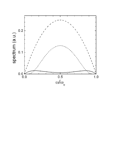
Figure 1: Spectral distribution of the emitted particles $dN/d\omega.$ For the horizontal scale, we divide the frequencies by the mechanical frequency $\omega_{0}.$ Dashed line: $\beta=0$ (Dirichlet case), solid line: $\beta\omega_{0}=1.7,$ dotted line $\beta\omega_{0}=5$.

A second important general property of the spectrum given by eq. (20) is the symmetry around $\omega=\omega_{0}/2:$ the spectrum is invariant under the replacement $\omega\rightarrow\omega_{0}-\omega.$ This is a signature that the particles are created in pairs, with frequencies such that their sum equals $\omega_{0}.$ Hence, for each particle created at frequency $\omega,$ there is a ‘twin’ particle created at frequency $\omega_{0}-\omega.$

Since Robin BC interpolate Dirichlet and Neumann ones, we may derive the spectra for these two cases by taking appropriate limits of eq. (20). For Dirichlet BC, we find

$$\left.\frac{dN}{d\omega}(\omega)\right|_{(D)}=\lim_{\beta\rightarrow 0}\frac{dN}{d\omega}(\omega)=\frac{(\delta q_{0})^{2}\,T}{2\pi}\,\omega(\omega_{0}-\omega)\,\Theta(\omega_{0}-\omega),$$ (21)

in agreement with Ref. [5]. For the Neumann BC ($\beta\rightarrow\infty$), we find the same spectrum, confirming the equivalence between Dirichlet and Neumann in the context of the dynamical Casimir effect in 1+1 dimensions [14].

For intermediate values of $\beta,$ the spectrum is always smaller than in the Dirichlet case for all values of $\omega.$ In fact, we may write the result of eq. (20) as

$$\frac{dN}{d\omega}(\omega)=\eta\,\frac{dN_{(D)}}{d\omega}(\omega),$$ (22)

where the reduction factor $\eta\leq 1$ is a function of $\beta\omega_{0}$ and $\omega/\omega_{0}.$ The reduction may be more severe near $\omega=\omega_{0}/2,$ which is the spectrum maximum in the Dirichlet case, for some values of $\beta\omega_{0}$. Hence, the Robin spectrum may develop global maxima near $\omega=0$ and $\omega=\omega_{0},$ as in the example shown in Fig. 1 (solid line), with $\beta\omega_{0}=1.7$. In this figure, we also plot the Dirichlet/Neumann spectrum (dashed line) and the Robin spectrum for $\beta\omega_{0}=5$ (dotted line). As discussed above, all curves are symmetric with respect to $\omega=\omega_{0}/2.$

The areas below the curves shown in Fig. 1 correspond to the total number of created particles. The figure already indicates that this number, to be discussed in the next section, may be considerably reduced (with respect to the Dirichlet case) for intermediate values of $\beta.$

4 Particle Creation Rate

The total number of created particles is given by

$$N=\int_{0}^{\omega_{0}}\frac{dN}{d\omega}(\omega)\,d\omega=\frac{\delta q_{0}^{2}\,T}{2\pi}\,\omega_{0}^{3}\,F(\beta\omega_{0}),$$ (23)

with

$$F(\xi)=\frac{\xi[4\xi+\xi^{3}+12\arctan(\xi)]-6(2+\xi^{2})\ln(1+\xi^{2})}{6\xi^{2}(4+\xi^{2})}$$ (24)

As expected for an open geometry (with a continuum of field modes), $N$ is proportional to the time $T,$ so that the particle creation rate $R\equiv N/T$ is the physically meaningful quantity. For the Dirichlet case, we take $F(\xi\rightarrow 0)=1/6,$ and then

$$R_{(D)}=\frac{\delta q_{0}^{2}\omega_{0}^{3}}{12\pi}.$$ (25)

For the Neumann case, we find the same result for the creation rate, since the spectrum is the same. Note that the rate increases with $\omega_{0}$ according to eq. (25) and vanishes (as required) in the static limit $\omega_{0}=0.$ This could have been anticipated since the particle creation is an effect of changing the BC nonadiabatically. However, for Robin BC the rate is not a monotonic function of $\omega_{0}.$ In Fig. 2, we plot the rate $R$ as a function of $\beta\omega_{0}$ (for a fixed $\beta$). $R$ decreases as $\omega_{0}$ varies from $1.3/\beta$ to the local minimum at $2.1/\beta.$

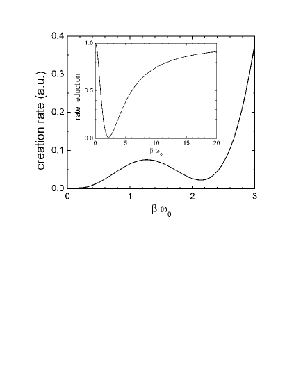
Figure 2: Total particle creation rate as a function of mechanical frequency (in units of $1/\beta$). Inset: ratio between creation rates for Robin and Dirichlet BC.

In the inset of Fig. 2, we plot the ratio $R/R_{(D)}=6F(\beta\omega_{0})\leq 1$ as a function of $\beta\omega_{0}.$ This ratio represents the reduction of the Dirichlet creation rate for a finite $\beta.$ It only depends on the the dimensionless variable $\beta\omega_{0},$ and goes asymptotically to one for $\beta\omega_{0}\gg 1,$ since the Neumann BC yields the same rate as the Dirichlet case. The reduction is maximum at $\beta\omega_{0}=2.2$. At this point, the creation rate is reduced to $1.3\%$ of the Dirichlet value .

We may also calculate the radiated energy from these results. Thanks to the symmetry of the spectrum around $\omega=\omega_{0}/2,$ we have

$$E=\int_{0}^{\omega_{0}}\frac{dN}{d\omega}(\omega)\,\hbar\omega\,d\omega=\frac{\hbar\omega_{0}}{2}\,N.$$ (26)

Combining with eq. (23), we find

$$E=\delta q_{0}^{2}\,T\,\hbar\omega_{0}^{4}\,F(\beta\omega_{0})/(4\pi).$$ (27)

This expression can be directly compared with the result for the Casimir force we have recently reported [12]. The force is written (in the Fourier domain) as ${\cal F}(\omega)=\chi(\omega)\delta Q(\omega)$ and its work on the slab is given in terms of the imaginary part of the susceptibility function $\chi(\omega)$:

$$W=-\frac{1}{\pi}\int_{0}^{\infty}d\omega\,\omega\,{\rm Im}\,\chi(\omega)\,|\delta Q(\omega)|^{2}.$$ (28)

For the quasi-sinusoidal motion considered here, we find, using eq. (19),

$$W=-\delta q_{0}^{2}\,T\,\omega_{0}\,{\rm Im}\,\chi(\omega_{0})/2.$$ (29)

The result for ${\rm Im}\,\chi(\omega_{0})$ derived in Ref. [12] can be cast in the form ${\rm Im}\,\chi(\omega_{0})=\hbar\omega_{0}^{3}F(\beta\omega_{0})/(2\pi).$ Then, the comparison of eqs. (27) and (29) yield $E=-W,$ so that the total radiated energy coincides with the negative of the work done on the slab by the Casimir force, as expected from energy conservation.

5 Conclusion

Dirichlet ($\beta\rightarrow 0$) and Neumann BC ($\beta\rightarrow\infty$) yield the same result for the spectrum of created particles. With the Robin BC, we are able to interpolate continuously between these two cases. For intermediate values of $\beta,$ the spectrum is always smaller than the Dirichlet/Neumann case, for all values of frequency.

In the range $1.2<\beta\omega_{0}<2.4$ the spectrum develops lateral peaks higher than the value at $\omega=\omega_{0}/2.$ This is also approximately the range in which the total creation rate (surprisingly) decreases with $\omega_{0}.$ This rate is reduced by up to $1.3\%$ of the Dirichlet/Neumann value, if the mechanical frequency is selected at $\omega_{0}=2.2/\beta.$ In other words, the coupling with the vacuum field state is considerably reduced if the slab oscillates at a frequency close to this value.

When considering the electromagnetic field and a plane mirror moving along its normal direction, the BC in the ideal case of perfect reflectors may be decomposed into Dirichlet and Neumann BC for each orthogonal polarization [15]. In 3+1 dimensions, the effect with Neumann BC is considerably larger than with Dirichlet BC, and it would be interesting to investigate the continuous transition between these two limiting cases.

Reflection by real metallic plates involve non-trivial frequency-dependent phase factors as in the case of Robin BC. The results of the present paper indicate that finite conductivity might yield a significant reduction of the magnitude of the dynamical Casimir effect.

This work was supported by the Brazilian agencies CNPq and FAPERJ. PAMN acknowledges Instituto do Milênio de Informação Quântica for partial financial support.

References

-
[1]
Fulling S A and Davies P C W 1976 Proc. R. Soc. London A 348 393
Jaekel M T and Reynaud S 1992 Quant. Opt. 4 39
Maia Neto P A and Reynaud S 1993 Phys. Rev. A 47 1639 - [2] Ford L H and Vilenkin A 1982 Phys. Rev. D 25 2569
- [3] Dalvit D A R and Maia Neto P A 2000 Phys. Rev. Lett. 84, 798
- [4] Special Issue on the Nonstationary Casimir effect and quantum systems with moving boundaries 2005 J. Opt. B: Quantum and Semiclass. Opt. 7
- [5] Lambrecht A, Jaekel M-T and Reynaud S 1996 Phys. Rev. Lett. 77 615
- [6] Maia Neto P A and Machado L A S 1996 Phys. Rev. A 54 3420
- [7] Mundarain D F and Maia Neto P A 1998 Phys. Rev. A 57 1379
- [8] Maia Neto P A 2005 J. Opt. B: Quantum and Semiclass. Opt. 7 S86
-
[9]
Dodonov V V and Klimov A B 1996 Phys. Rev. A 53 2664
Crocce M, Dalvit D A R and Mazzitelli F D 2001 Phys. Rev. A 64 013808
Schaller G, Schützhold R, Plunien G and Soff G 2002 Phys. Rev. A 66 023812 - [10] Crocce M, Dalvit D A R, Lombardo F C and Mazzitelli F D 2005 J. Opt. B: Quantum and Semiclass. Opt. 7 S32
- [11] Eberlein C 1996 Phys. Rev. Lett. 76 3842
- [12] Mintz B, Farina C, Maia Neto P A and Rodrigues R 2006 J. Phys. A 39 6559
- [13] Chen G and Zhou J 1993 Vibration and Damping in Distributed Systems vol I (Boca Raton, FL:CRC) p15
- [14] Alves D T, Farina C and Maia Neto P A 2003 J. Phys. A 36 1133
- [15] Maia Neto P A 1994 J. Phys. A 27 2167.