Lab/UFR-HEP0601/GNPHE/0601/VACBT/0601

D-string fluid in conifold:
II. Matrix model for D-droplets on $\mathbb{S}^{3}$ and $\mathbb{S}^{2}$

Abstract

Motivated by similarities between Fractional Quantum Hall (FQH) systems and aspects of topological string theory on conifold, we continue in the present paper our previous study (hep-th/0604001, hep-th/0601020) concerning FQH droplets on conifold. Here we focus our attention on the conifold sub-varieties $\mathbb{S}^{3}$ and $\mathbb{S}^{2}$ and study the non commutative quantum dynamics of D1 branes wrapped on a circle. We give a matrix model proposal for FQH droplets of $N$ point like particles on $\mathbb{S}^{3}$ and $\mathbb{S}^{2}$ with filling fraction $\nu=\frac{1}{k}$. We show that the ground state of droplets on $\mathbb{S}^{3}$ carries an isospin $j=k\frac{N\left(N-1\right)}{2}$ and gives remarkably rise to $2j+1$ droplets on $\mathbb{S}^{2}$ with Cartan-Weyl charge $\left|j_{z}\right|\leq j$.

Key words:   
Fractional quantum Hall droplets, D1 branes, matrix model and non commutative geometry, conifold, topological string on $T^{\ast}\mathbb{S}^{3}$.

1 Introduction

Recently a matrix model proposal for Laughlin fluid on real 2-sphere $\mathbb{S}^{2}$ with a radius $R$ has been studied in [1]. Starting from the field action of a fractional quantum Hall (FQH) particle moving on $\mathbb{S}^{2}$ with Kahler potential $K\left(z,\overline{z}\right)=\ln\left(1+\overline{z}z\right)$; then promoting the coordinate positions $\left\{z_{a},\overline{z}_{a},\text{ }0\leq a\leq N\right\}$ of the FQH droplet $N$ particles into $N\times N$ matrix fields $Z_{b}^{a}=Z_{b}^{a}\left(t\right)$ and its adjoint conjugate $Z_{a}^{+b}=Z_{a}^{+b}\left(t\right)$, Morariu and Polychronakos (MP) proposed that the lagrangian density $\mathcal{L}_{MP}\mathcal{=L}(Z,Z^{+},\mathcal{A})$ describing a such system reads as,

$$\mathcal{L}_{MP} = iB\mathrm{Tr}\left[R^{2}(1+ZZ^{+})^{-1}\left(\mathcal{D}_{t}Z\right)Z^{+}\right]$$

$$-iB\mathrm{Tr}\left[R^{2}\left(\mathcal{D}_{t}Z\right)^{+}(1+ZZ^{+})^{-1}Z\right]$$

$$+\mathrm{Tr}\left[\Psi^{+}\left(i\frac{d\Psi}{dt}+\mathcal{A}\Psi\right)\right]-B\theta\mathrm{Tr}\left(\mathcal{A}\right),$$

with an ordering in which $Z$ and $Z^{\dagger}$ alternate. In this relation the constant $B$ is the magnitude of the usual background magnetic field, the $N\times N$ hermitian matrix $\mathcal{A}=\mathcal{A}\left(t\right)$ is the gauge field capturing the fluid incompressibility constraint and $\mathcal{D}_{t}Z=\frac{dZ}{dt}-i\left[\mathcal{A},Z\right]$. The $N$ component vector $\left(\Psi^{a}\right)$ is the Polychronakos field with adjoint conjugate $\left(\Psi_{a}^{+}\right)$ and $\theta$ is the non commutativity parameter related to the magnetic field as $B\theta=k$ with $k$ a positive definite integer [2]. Recall that the integer $k$ appears in continuous gauge field formulation as the level of non commutative $U\left(1\right)$ Chern Simons gauge model and $\nu=\frac{1}{k}$ is the filling fraction of Laughlin state; for related studies and generalizations see also [3]-[11].

In the present paper, we consider an alternative matrix model approach for FQH droplets on the spheres $\mathbb{S}^{3}$ and $\mathbb{S}^{2}$ with filling fraction $\nu$. This study, which is also motivated from the analysis of dynamics of D-string fluid in conifold [12]-[13], is based on a constrained method and deals with the spheres as hypersurfaces in $\mathbb{R}^{4}$. The matrix field action modeling the system is built as follows:

(1) First, we consider matrix model for FQH droplet on the 3-sphere $\mathbb{S}^{3}\simeq SU\left(2\right)$ by using Lagrange method for dealing with constraint eqs. In this model, the 3-sphere $\mathbb{S}^{3}$ is thought of as a real hypersurface $\left|x\right|^{2}+\left|y\right|^{2}=R^{2}$ embedded in $\mathbb{C}^{2}\simeq\mathbb{R}^{4}$ and the corresponding matrix field action $\mathcal{S}_{3}$ has the following field dependence $\mathcal{S}_{3}=\mathcal{S}_{3}\left[X,Y,\mathcal{A},\mathcal{C}\right]$ where the gauge field $\mathcal{A}=\mathcal{A}\left(t\right)$ captures fluid incompressibility condition and plays the same role as in eq(1). After matrix elevation of the coordinate positions $\left\{x_{a}\right\}\rightarrow X$ and $\left\{y_{a}\right\}\rightarrow Y$, the resulting matrix hypersurface elevating the 3-sphere namely,

$$\mathrm{Tr}\left(X^{+}X+Y^{+}Y\right)=R^{2}N,$$ (1.2)

is treated as a constraint eq and is implemented in the field action via an extra gauge field $\mathcal{C}=\mathcal{C}\left(t\right)$.

(2) Then starting from the matrix field action $\mathcal{S}_{3}$, we use the coset realization $SU\left(2\right)/U_{C}\left(1\right)$ of $\mathbb{S}^{2}\simeq\mathbb{C}\mathbb{P}^{1}$ to deduce the matrix model proposal for FQH droplet on the 2-sphere. The resulting matrix field action $\mathcal{S}_{2}$ has now the matrix field dependence; $\mathcal{S}_{2}=\mathcal{S}_{2}\left[X,Y,\mathcal{A},\mathcal{B},\mathcal{C}\right]$. The extra gauge field $\mathcal{B}=\mathcal{B}\left(t\right)$ captures the coset gauge symmetry,

$$X^{\prime}\left(t\right) = e^{i\varphi\left(t\right)}X\left(t\right),$$

$$Y^{\prime}\left(t\right) = e^{-i\varphi\left(t\right)}Y\left(t\right).$$ (1.3)

In the language of $SU\left(2\right)$ group generated by the usual 3-operators $\mathbf{J}_{\pm}$ and $\mathbf{J}_{0}$ ( see also eqs(4.17-4.18)), this reduction from $\mathbb{S}^{3}$ down to $\mathbb{S}^{2}$ corresponds just to fixing the charge of the $U_{C}\left(1\right)$ Cartan Weyl operator $\mathbf{J}_{0}$. Quantum mechanically, this means that wave functions $|\Phi>$ describing FQH droplets on $\mathbb{S}^{2}$ should obey, amongst others, the following constraint eq

$$\mathbf{J}_{0}|\Phi>=j_{z}|\Phi>,$$ (1.4)

where $j_{z}=mN$ is a relative integer. As an immediate consequence; the wave functions describing FQH droplets on the 3-sphere are given by $SU\left(2\right)$ highest state representations which we denote as,

$$|\Phi>=\left(\text{ \ }|\Phi_{j,j_{z}}>\text{ \ }\right),\qquad\left|j_{z}\right|\leq j,$$ (1.5)

with highest weight $j=lN$. This result will be proved later on. The condition (1.4) corresponds then to picking up one of the basis states of above isospin $j$ representation. Eqs(1.4-1.5) gives a remarkable link between FQH systems on the spheres $\mathbb{S}^{3}$ and $\mathbb{S}^{2}$. Indeed, a FQH droplet on the 3-sphere carries a isospin $j$ and then is made of $\left(2j+1\right)$ FQH droplets on $\mathbb{S}^{2}$.

Note that our approach to FQH droplets on the 2-sphere may be viewed as a linearized description of MP model. In other words, this way of doing avoids the high non linearity in the matrix field embodied by the factors $(1+ZZ^{+})^{-1}$ and $(1+Z^{+}Z)^{-1}$ of eq(1) which have infinite expansion in $ZZ^{+}$ and $Z^{+}Z$ respectively. This aim is achieved by introducing two extra gauge fields. The new matrix field action $\mathcal{S}_{2}\left[X,Y,\mathcal{A},\mathcal{B},\mathcal{C}\right]=\int dt\mathcal{L}_{2}$ with

$$\mathcal{L}_{2} = -iB\mathrm{Tr}\left[X^{+}\frac{dX}{dt}+Y^{+}\frac{dY}{dt}\right]+B\mathrm{Tr}\left[\mathcal{A}\left(\left[X^{+},X\right]+\left[Y^{+},Y\right]-\frac{k}{B}\right)\right]$$

$$-B\mathrm{Tr}\left[\mathcal{C}\left(\left(X^{+}X+Y^{+}Y\right)-\frac{l}{B}\right)\right]-B\mathrm{Tr}\left[\mathcal{B}\left(\left(X^{+}X-Y^{+}Y\right)-\frac{m}{B}\right)\right]$$

involves three kinds of constraint eqs: (i) The usual fluid incompressibility condition captured by the gauge field $\mathcal{A}$. (ii) The coordinate restriction, describing the embedding $\mathbb{S}^{3}$ into $\mathbb{R}^{4}$, and captured by the gauge field $\mathcal{C}$. (iii) Reduction of $\mathbb{S}^{3}$ down to $\mathbb{S}^{2}$ using the standard fibration $\mathbb{S}^{3}\sim\mathbb{S}^{1}\times\mathbb{S}^{2}$; the corresponding constraint eq is captured by the gauge field $\mathcal{B}$.

An other advantage of our method consists in building FQH extensions based on geometries going beyond $\mathbb{S}^{2}$. A class of these generalizations is given by the following special extensions: ($\mathbf{\alpha}$) the real 3-sphere $\mathbb{S}^{3}$ with matrix field action $\mathcal{S}_{3}=\mathcal{S}_{2}|_{\mathcal{B}=0}$ considered in this paper; see section 3. ($\mathbf{\beta}$) The K3 complex surface viewed as $T^{\ast}\mathbb{S}^{2}$ and conifold $T^{\ast}\mathbb{S}^{3}$ under investigation in [14].

The presentation of this paper is as follows: In section 2, we describe FQH droplets on $\mathbb{S}^{3}$ and $\mathbb{S}^{2}$ and derive the corresponding constraint equations. In section 3, we develop our matrix model proposal of FQH droplets on the spheres and analyse the structure of the matrix constraint eqs. In section 4, we consider the quantum version and build the droplet ground state. Last section is devoted to conclusion and outlook.

2 $\mathbb{S}^{3}$ and $\mathbb{S}^{2}$ Conifold sub-varieties in $\mathbb{C}^{2}$

We start this section by presenting briefly the coordinate frame we shall use to describe the spheres $\mathbb{S}^{3}$ and $\mathbb{S}^{2}$. Then we derive the constraint eqs of the system. There are different ways to parameterize these spheres; but here we will think about them as hypersurfaces in the complex space $\mathbb{C}^{2}$ $\left(\simeq\mathbb{R}^{4}\right)$ with holomorphic coordinates $x$ and $y$. This choice, which is motivated by the use of manifest isometry, gives also an issue to deal with possible extensions involving K3 and conifold [13].
In the last part, we describe the classical field actions of particles moving on the spheres, embedded into $\mathbb{C}^{2}$, in presence of a constant and strong external magnetic field.

2.1 FQH constraint eqs on spheres

Recall that fluid incompressibility constraint is essential in the field theoretic modeling of FQH systems. This constraint eq, related to the fluid approximation, plays a central role in understanding the quantum dynamics. For FQH systems on non flat manifolds, one should also worry about curvature effect.

In the present case, we want to study FQH systems on the spheres $\mathbb{S}^{3}$ and $\mathbb{S}^{2}$ embedded in $\mathbb{C}^{2}$. Since these geometries are non flat, we have then extra constraint relations besides the usual one dealing with fluid incompressibility. In this subsection, we want to identify these constraint relations.

2.1.1 $\mathbb{S}^{3}$ case

Starting from the complex two dimension space $\mathbb{C}^{2}$ with local holomorphic coordinates $x$ and $y$, we can realize the 3-sphere $\mathbb{S}^{3}$ as a real hypersurface $H_{\mathop{\mathrm{r}eal}}=H_{\mathop{\mathrm{r}eal}}\left(x,y,\overline{x},\overline{y}\right)$ embedded in $\mathbb{C}^{2}$. In practice this is achieved by restricting the complex coordinates $\left(x,y\right)$ and their complex conjugates to obey the following constraint relation,

$$H_{\mathop{\mathrm{r}eal}}\left(x,y,\overline{x},\overline{y}\right):\qquad x\overline{x}+y\overline{y}=\left|x\right|^{2}+\left|y\right|^{2}=R^{2},$$ (2.1)

where $R$ is the radius of the sphere. For later use note that eq(2.1), may be put into various forms. An interesting way is the one using representations of the $SU\left(2\right)$ isometry of $\mathbb{S}^{3}$. For this aim we use the isospinors

$$z^{i}=\left(x,y\right),\qquad\overline{z}_{i}=\overline{\left(z^{i}\right)}=\left(\overline{x},\overline{y}\right),\qquad i=1,2.$$ (2.2)

The usual $SU\left(2\right)$ invariant antisymmetric tensor $\varepsilon^{ij}$ and its inverse $\varepsilon_{ji}$ raise and lower the $SU\left(2\right)$ indices. So, eq(2.1) reads also as follows,

$$H_{\mathop{\mathrm{r}eal}}\left(z,z\right):\qquad\sum_{i=1}^{2}z^{i}\overline{z}_{i}=R^{2}.$$ (2.3)

This relation is invariant under the following manifest $SU\left(2\right)$ rotations $z^{i}=M_{j}^{i}z^{j}$ and $\overline{z}_{i}=\overline{z}_{k}M_{i}^{\ast k}$ with $M_{i}^{\ast k}M_{j}^{i}=\delta_{j}^{k}$ and $\det M=1$.  We also have the following operators,

$$\mathrm{J}_{+} = z^{i}\frac{\partial}{\partial\overline{z}^{i}},$$

$$\mathrm{J}_{-} = \overline{z}^{i}\frac{\partial}{\partial z^{i}},$$ (2.4)

$$\mathrm{J}_{0} = \left(z^{i}\frac{\partial}{\partial z^{i}}-\overline{z}^{i}\frac{\partial}{\partial\overline{z}^{i}}\right),$$

satisfying the usual commutation relations of the $SU\left(2\right)$ algebra,

$$\left[\mathrm{J}_{0},\text{{J}}_{+}\right] = 2\text{{J}}_{+},$$

$$\left[\mathrm{J}_{0},\mathrm{J}_{-}\right] = -2\mathrm{J}_{-},$$ (2.5)

$$\left[\mathrm{J}_{+},\mathrm{J}_{-}\right] = \mathrm{J}_{0}.$$

Later on ( see section 4), we shall use creation and annihilation operators of the quantum matrix model proposal to represent this group symmetry. Now let us consider a particle with coordinate position $x\left(t\right),$ $y\left(t\right)$ and $\overline{x}\left(t\right),$ $\overline{y}\left(t\right)$ moving in the complex space $\mathbb{C}^{2}$. The restriction to a motion on the 3-sphere is achieved by requiring

$$x\left(t\right)\overline{x}\left(t\right)+y\left(t\right)\overline{y}\left(t\right)=R^{2},$$ (2.6)

at every moment t.
For a set of $N$ particles described by $x_{a}\left(t\right),$ $y_{a}\left(t\right)$ and $\overline{x}_{a}\left(t\right),$ $\overline{y}_{a}\left(t\right)$ with $a=1,...,N$, moving in the complex space $\mathbb{C}^{2}$, the above relation extends as follows,

$$x_{a}\left(t\right)\overline{x}_{a}\left(t\right)+y_{a}\left(t\right)\overline{y}_{a}\left(t\right)=R^{2},\qquad a=1,...,N.$$ (2.7)

Besides fluid incompressibility constraint relation, (2.7) represents an extra condition restricting the dynamics of $N$ particles on $\mathbb{C}^{2}$ down to the 3-sphere. We shall turn to this condition later on; for the moment let us consider the constraint eqs for the 2-sphere embedded in $\mathbb{C}^{2}$ using Hopf fibration of $\mathbb{S}^{3}$.

2.1.2 $\mathbb{S}^{2}$ as reduced $\mathbb{S}^{3}$

There are various ways to parameterize $\mathbb{S}^{2}$; one of these realizations considered recently in [1] is given by the stereographic coordinate variables using Kahler potential of $\mathbb{S}^{2}\simeq C\mathbb{P}^{1}$. An other interesting coordinate frame, which we shall use here below, rests on embedding $\mathbb{S}^{2}$ in the complex two space $\mathbb{C}^{2}$.

To embed $\mathbb{S}^{2}$ in the complex space $\mathbb{C}^{2}$, one restricts the complex coordinates $\left(x,y\right)$ to the real hypersurface (2.1) and uses the fibration $\mathbb{S}^{3}\simeq\mathbb{S}^{1}\times\mathbb{S}^{2}$ to restrict further the 3-sphere down to $\mathbb{S}^{2}$. This is achieved by the identification

$$x^{\prime}\equiv e^{i\varphi}x,\qquad y^{\prime}\equiv e^{-i\varphi}y,$$ (2.8)

where $\varphi$ is the group parameter of $U_{C}\left(1\right)$ Cartan abelian sub-symmetry of the $SU\left(2\right)$ isometry of the 3-sphere. From group theoretic view, this identification corresponds to starting from $\mathbb{S}^{3}\simeq SU\left(2\right)$ and performing the coset,

$$SU\left(2\right)\qquad\rightarrow\qquad SU\left(2\right)/U_{C}\left(1\right).$$ (2.9)

Notice that without the identification (2.8), the hypersurface $H_{\mathop{\mathrm{r}eal}}\left(x,y,\overline{x},\overline{y}\right)$ would describe a $\mathbb{S}^{3}$ sphere realized as the fibration of $\mathbb{S}^{1}$ over $\mathbb{S}^{2}$.
For a system of $N$ particles with coordinate positions $x_{a}\left(t\right),$ $y_{a}\left(t\right)$ and $\overline{x}_{a}\left(t\right),$ $\overline{y}_{a}\left(t\right)$, we have in addition to eq(2.7) the following constraint relation,

$$x_{a}^{\prime}\left(t\right)=e^{i\varphi\left(t\right)}x_{a}\left(t\right),\qquad y_{a}^{\prime}\left(t\right)=e^{-i\varphi\left(t\right)}y_{a}\left(t\right),\qquad a=1,...,N,$$ (2.10)

where the phase $\varphi=\varphi\left(t\right)$ is time dependent. Therefore, eqs(2.1-2.8) form a set of two constraint relations; the first one reduces the space $\mathbb{C}^{2}\sim\mathbb{R}^{4}$ into the real 3-sphere $\mathbb{S}^{3}$ and the second reduces $\mathbb{S}^{3}$ down to the 2-sphere $\mathbb{S}^{2}$.

2.2 Classical field action on $\mathbb{S}^{3}$

Following [2], the field action $S_{3}=\int dt$ $\mathrm{L}_{3}$, describing a particle moving on the real 3-sphere $\mathbb{S}^{3}\sim SU\left(2\right)$ and taken in the condition of FQH systems, is obtained as follows. Start from the lagrangian density $\mathrm{L}_{4}=\mathrm{L}_{4}\left(x,\overline{x},y,\overline{y}\right)$ of a FQH particle moving on the complex two dimension space $\mathbb{C}^{2}\sim\mathbb{R}^{4}$ which reads as follows,

$$\mathrm{L}_{4}=-\frac{iB}{2}\left[\left(\overline{x}\frac{dx}{dt}-x\frac{d\overline{x}}{dt}\right)+\left(\overline{y}\frac{dy}{dt}-y\frac{d\overline{y}}{dt}\right)\right],$$ (2.11)

which, by using the isodoublet coordinates $z^{i}$, reads also as,

$$dt\text{ }\mathrm{L}_{4}=-\frac{iB}{2}\left(\overline{z}_{i}dz^{i}-z^{i}d\overline{z}_{i}\right).$$ (2.12)

In eq(2.11), the field variables $x$ and $y$ are the holomorphic coordinate variables of $\mathbb{C}^{2}$. To get the lagrangian density $\mathrm{L}_{3}$ describing the dynamics of this FQH particle; but now restricted to moving on $\mathbb{S}^{3}$, one should impose the constraint eq

$$B\left(x\overline{x}+y\overline{y}\right)=l$$ (2.13)

where, because of non commutativity requirement, we have set

$$BR^{2}=l,\qquad R^{2}=\frac{l}{B},$$ (2.14)

with $l$ a positive integer. This condition can be implemented in the above lagrangian density $\mathrm{L}_{4}$ as usual by using the Lagrange method. As such the lagrangian density $\mathrm{L}_{3}$ describing the classical motion of the particle on the 3-sphere reads as,

$$\mathrm{L}_{3}=-B\left[\overline{x}\left(i\frac{dx}{dt}+\mathrm{C}x\right)+\overline{y}\left(i\frac{dy}{dt}+\mathrm{C}y\right)-\mathrm{C}\frac{l}{B}\right].$$ (2.15)

In this equation, the real field $\mathrm{C}=\mathrm{C}\left(t\right)$ is the Lagrange gauge field capturing the constraint eq(2.13) for embedding the hypersurface $\mathbb{S}^{3}$ into $\mathbb{C}^{2}$. By minimizing $\mathrm{L}_{3}$ with respect to the field $\mathrm{C}$, we get precisely the constraint eq(2.13); i.e,

$$\frac{\partial\mathrm{L}_{3}}{\partial\mathrm{C}}=-B\left(x\overline{x}+y\overline{y}\right)+l=0.$$ (2.16)

As we see, eq(2.15) is an abelian one dimensional gauge theory with target space $\mathbb{C}^{2}$ and gauge covariant derivatives $\mathcal{D}_{t}z=\left(\frac{dz}{dt}-i\mathrm{C}z\right)$ where $z$ stands for $x\left(t\right)$ and $y\left(t\right)$. The gauge transformations leaving $\mathrm{L}_{3}$ invariant read then as follows,

$$z^{\prime}=e^{i\lambda}z,\qquad\mathrm{C}^{\prime}=\mathrm{C}+\frac{d\lambda}{dt},$$ (2.17)

where $\lambda=\lambda\left(t\right)$ is the gauge group parameter.

Starting from the above relations, we consider now the classical system of N FQH particles on $\mathbb{S}^{3}$. Using the $z_{a}^{i}=\left(x_{a},y_{a}\right)$ and $\overline{z}_{ia}=\left(\overline{x}_{a},\overline{y}_{a}\right)$ doublets constrained as,

$$B\left(x_{a}\overline{x}_{a}+y_{a}\overline{y}_{a}\right)=l,\qquad a=1,...,N,$$ (2.18)

the lagrangian density describing the classical dynamics of these particles on the 3-sphere reads then as

$$\mathrm{L}_{3}\left(z,\overline{z},\mathrm{C}\right)=-B\sum_{a=1}^{N}\left[i\overline{z}_{ia}\mathcal{D}_{t}z^{ia}-\mathrm{C}_{a}\frac{l}{B}\right],$$ (2.19)

where the gauge covariant derivatives $\mathcal{D}_{t}z^{ia}$ is as before and where summation over the $SU\left(2\right)$ index is understood. From this lagrangian density, the conjugate momenta $\pi_{ia}\left(t\right)$ of the field variable $z^{ia}$ is equal to $\pi_{ia}=-iB\overline{z}_{ia}$ and the corresponding Poisson brackets are,

$$\left\{z^{ia},\overline{z}_{jb}\right\}_{PB} = \frac{i}{B}\delta_{j}^{i}\delta_{b}^{a},$$

$$\left\{z^{ia},z^{jb}\right\}_{PB} = \left\{\overline{z}_{ia},\overline{z}_{jb}\right\}_{PB}=0,$$ (2.20)

where

$$\left\{F,G\right\}_{PB}=\sum_{l,e}\left(\frac{\partial F}{\partial z^{le}}\frac{\partial G}{\partial\pi_{le}}-\frac{\partial F}{\partial\pi_{le}}\frac{\partial G}{\partial z^{le}}\right).$$ (2.21)

In the fluid approximation requiring a large number $N$ of particles, the previous coordinate position variables $z_{a}^{i}$ and $\overline{z}_{ia}$ are promoted to highest dimensional fields as shown below,

$$\left\{z_{a}^{i}\left(t\right),\text{ {C}}_{a}\left(t\right)\text{, }{\small 1\leq a\leq N}\right\}\qquad\rightarrow\qquad z^{i}\left(t;\tau,\overline{\tau},\sigma,\overline{\sigma}\right),\text{ {C}}\left(t;\tau,\overline{\tau},\sigma,\overline{\sigma}\right),$$ (2.22)

or by using the $x$ and $y$ variables,

$$\left\{x_{a}\left(t\right),\text{ }y_{a}\left(t\right)\text{, }{\small 1\leq a\leq N}\right\}\qquad\rightarrow\qquad x\left(t;\tau,\overline{\tau},\sigma,\overline{\sigma}\right),\text{ }y\left(t;\tau,\overline{\tau},\sigma,\overline{\sigma}\right).$$ (2.23)

In this approximation, the constraint relation capturing the incompressibility condition of the FQH fluid is translated into a condition on the Jacobian $\mathcal{J}_{ac}$ of the transformation,

$$\tau\qquad \rightarrow \qquad x\left(\tau,\sigma;\overline{\tau},\overline{\sigma}\right),$$

$$\sigma\qquad \rightarrow \qquad y\left(\tau,\sigma;\overline{\tau},\overline{\sigma}\right),$$ (2.24)

together with similar transformations for the complex conjugate partners. Fluid incompressibility requires that the absolute value

$$\left|\mathcal{J}_{ac}\right|=\left|\frac{\partial^{4}\left(x,y;\overline{x},\overline{y}\right)}{\partial^{4}\left(\tau,\sigma;\overline{\tau},\overline{\sigma}\right)}\right|$$ (2.25)

should satisfy $\left|\mathcal{J}_{ac}\right|=1$. By expliciting (2.25), we see that $\mathcal{J}_{ac}$ is a polynom $P=P\left(\partial z^{i},\partial\overline{z}_{i}\right)$ of fourth order in the gradient of the fields;

$$\mathcal{J}_{ac} = \left\{x,\overline{x}\right\}_{\tau\overline{\tau}}\left\{y,\overline{y}\right\}_{\sigma\overline{\sigma}}+\left\{x,\overline{x}\right\}_{\sigma\overline{\sigma}}\left\{y,\overline{y}\right\}_{\tau\overline{\tau}}$$

$$+\left\{x,\overline{x}\right\}_{\sigma\tau}\left\{y,\overline{y}\right\}_{\overline{\tau}\overline{\sigma}}+\left\{x,\overline{x}\right\}_{\overline{\sigma}\overline{\tau}}\left\{y,\overline{y}\right\}_{\tau\sigma}$$

$$+\left\{x,\overline{x}\right\}_{\tau\overline{\sigma}}\left\{y,\overline{y}\right\}_{\overline{\tau}\sigma}+\left\{x,\overline{x}\right\}_{\overline{\tau}\sigma}\left\{y,\overline{y}\right\}_{\tau\overline{\sigma}},$$

where $\left\{f,g\right\}_{\alpha\beta}$ are defined by $\left(\frac{\partial f}{\partial\alpha}\frac{\partial g}{\partial\beta}-\frac{\partial f}{\partial\beta}\frac{\partial g}{\partial\alpha}\right)$. This Jacobian is quadratic in the Poisson brackets and involves the sum of six terms. To deal with the fluid incompressibility condition $\left|\mathcal{J}_{ac}\right|=1$, we begin by simplifying the above expression by restricting the coordinate transformations (2.24) to the sub-class,

$$\tau\qquad \rightarrow \qquad x\left(\tau,\overline{\tau}\right),$$

$$\sigma\qquad \rightarrow \qquad y\left(\sigma,\overline{\sigma}\right).$$ (2.27)

With these particular class of general coordinate transformations, eq(2.2) simplifies to $\mathcal{J}_{ac}=\left\{x,\overline{x}\right\}_{\tau\overline{\tau}}\left\{y,\overline{y}\right\}_{\sigma\overline{\sigma}}$ and the fluid incompressibility condition reduces to the following relation,

$$\left\{x,\overline{x}\right\}_{PB}\left\{y,\overline{y}\right\}_{PB}=-\theta^{2},$$ (2.28)

where $\theta$ is the usual non commutative coordinates parameters with $\theta B=k$. This constraint eq can be solved as $\left\{x,\overline{x}\right\}_{PB}=i\theta$ and $\left\{y,\overline{y}\right\}_{PB}=i\theta$ or equivalently by using the $SU\left(2\right)$ doublets as follows,

$$\left\{\overline{z}_{i},z^{j}\right\}_{PB}=-i\theta\delta_{i}^{j}.$$ (2.29)

These special constraint relations constitute then the condition for fluid incompressibility; they have as usual a non commutative geomerty interpretation. Implementing, this constraint eq into eqs(2.19) by using the Lagrange method, we get the field action $\mathrm{S}_{3}=\mathrm{S}_{3}\left(z,\overline{z},\mathrm{C,A}\right)$ for incompressible fluid running on the 3-sphere,

$$\mathrm{S}_{3}=-B\int dtd^{2}\tau d^{2}\sigma\left[i\overline{z}_{i}\mathcal{\nabla}_{t}z^{i}-\mathrm{C}\frac{l}{B}-\mathrm{A}\frac{k}{B}\right],$$ (2.30)

where we have set,

$$\mathcal{\nabla}_{t}z^{i}=\mathcal{D}_{t}z^{i}-i\left\{\mathrm{A},z^{i}\right\}_{PB},$$ (2.31)

and where $\theta$ is the non commutative parameter considered previously. The gauge field $\mathrm{A}=\mathrm{A}\left(t,\tau,\sigma;\overline{\tau},\overline{\sigma}\right)$ is a real gauge field capturing the fluid incompressibility constraint equation.

3 Matrix model of droplets on $\mathbb{S}^{3}$ and $\mathbb{S}^{2}$

In this section, we develop a matrix model proposal of fractional quantum Hall droplets on the real spheres $\mathbb{S}^{3}$ and $\mathbb{S}^{2}$. The gauge field theoretical method developed here can be also viewed as an other way to approach FQH droplets on $\mathbb{S}^{2}$ other than the one considered recently in [1] by using stereographic coordinates. It has moreover the property of giving a unified description of FQH systems on $\mathbb{S}^{3}$ and $\mathbb{S}^{2}$ and a priori D-string droplets on conifold which is under investigation in [14]; for a Chern-Simons like description see [13].

To begin note that using the spheres realizations (2.1,2.8), one can parameterize the FQH droplet $N$ particles moving on $\mathbb{S}^{3}$, up to the identification (2.8) on $\mathbb{S}^{2}$, as follows,

$$x_{a} = x_{a}\left(t\right),\qquad\overline{x}_{a}=\overline{x}_{a}\left(t\right),$$

$$y_{a} = y_{a}\left(t\right),\qquad\overline{y}_{a}=\overline{y}_{a}\left(t\right),$$ (3.1)

with $a=1,...,N$ indexing the set of particles. Recall that the restriction of the above FQH particle trajectories on $\mathbb{C}^{2}$ down to the real three dimension hypersurface $\mathbb{S}^{3}$ is given by the following constraint relations (2.18).

3.1 Matrix field variables

In the non commutative $N\times N$ matrix description of the FQH system on the spheres $\mathbb{S}^{3}$ and $\mathbb{S}^{2}$, one proceeds more or less as usual. First, one elevates the commuting coordinate position variables $\left\{z_{a}^{i}\left(t\right),\text{ }\overline{z}_{i}^{a},\text{ }1\leq a\leq N\right\}$ of the ambiant space $\mathbb{C}^{2}$ into $N\times N$ complex matrices as shown below,

$$X_{0}=\left(\begin{array}[]{cccc}x_{1}&0&.&0\\ 0&x_{2}&.&0\\ .&.&.&.\\ 0&0&.&x_{N}\end{array}\right),\qquad Y_{0}=\left(\begin{array}[]{cccc}y_{1}&0&.&0\\ 0&y_{2}&.&0\\ .&.&.&.\\ 0&0&.&y_{N}\end{array}\right)$$ (3.2)

together with the adjoint matrices $X_{0}^{+}$ and $Y_{0}^{+}$. This is not the unique way to do, since there are also other equivalent matrices $X$ and $Y$ related to (3.2) by using similarity transformations. Second, in terms of the diagonal matrices (3.2), the constraint relations (2.18) become,

$$B\left(X_{0}^{+}X_{0}+Y_{0}^{+}Y_{0}\right)=l\text{ }\mathrm{I}_{id}.$$ (3.3)

The hermiticity property of $X^{+}X$ and $Y^{+}Y$ gives the general picture of eq(3.3) where $X$ and $Y$ are no longer diagonal. This is ensured by a $U\left(N\right)$ similarity transformation,

$$P:X_{0}^{+}X_{0}\qquad\rightarrow\qquad X^{+}X=P^{+}\left(X_{0}^{+}X_{0}\right)P,$$ (3.4)

with the $N\times N$ matrix $P$ satisfies $P^{+}P=PP^{+}=\mathrm{I}_{id}$. The same may be also done for $Y^{+}Y$. Note in passing that this $U\left(N\right)$ transformation is in fact a special solution involving adjoint representation of the $U\left(N\right)$ group; for a more general description involving the $U\left(N\right)\times U\left(N\right)$ gauge symmetry as well as bi-fundamental representations, see [15].

The third step towards the building of the matrix model is to note that FQH system $\left\{z_{a}^{i}\left(t\right),\text{ }\overline{z}_{i}^{a}\left(t\right),\text{ }1\leq a\leq N\right\}$ constrained as in eqs(2.18) can be described by using $N\times N$ matrices $X$ and $Y$ as well as their adjoints. These matrices encode the coordinate positions of the FQH droplet and the extra degrees of freedom are eliminated at the level of the field action by imposing the $U\left(N\right)$ symmetry,

$$\left(X\text{, }Y\right)\qquad \rightarrow \qquad\left(P^{+}XP\text{, }P^{+}YP\right)$$

$$\left(X^{+}\text{, }Y^{+}\right)\qquad \rightarrow \qquad\left(P^{+}X^{+}P\text{, }P^{+}Y^{+}P\right).$$ (3.5)

as well as,

$$B\mathrm{Tr}\left(X^{+}X+Y^{+}Y\right)=lN,$$ (3.6)

for FQH on the 3-sphere $\mathbb{S}^{3}$. We will show below that the reduction down to the $\mathbb{S}^{2}$ geometry requires moreover the condition,

$$B\mathrm{Tr}\left(X^{+}X-Y^{+}Y\right)=mN,$$ (3.7)

where $m$ is a relative integer. Combing eqs(3.6) and (3.7), one has

$$B\mathrm{Tr}\left(Y^{+}Y\right)=\frac{l-m}{2}N$$ (3.8)

and

$$B\mathrm{Tr}\left(X^{+}X\right)=\frac{l+m}{2}N.$$ (3.9)

Positivity of these quantities leads to the condition,

$$m\text{ }N\text{ }\leq\text{ }l\text{ }N.$$ (3.10)

This relation recalls the usual $SU\left(2\right)$ spin projection inequality,

$$j_{z}\text{ }\leq\text{ }j.$$ (3.11)

Note that emergence of such $SU\left(2\right)$ relation is not a strange thing. We will derive it later on; but for the moment note that this is a previsible property since the matrix variables X and Y carry a $SU\left(2\right)$ charge.

3.2 Lagrangian density

The non commutative matrix field lagrangian density describing the above FQH droplet on the 2-sphere is obtained by following the steps:

(a) Implement the matrix elevation $x\rightarrow X$ and $y\rightarrow Y$ into the field action eq(2.11). This gives a matrix field action $\mathcal{S}_{4}=\mathcal{S}_{4}\left[X,Y\right]$ on $\mathbb{C}^{2}$.

(b) Embed the constraint eq(2.18) for droplet dynamics on the 3-sphere by using a Lagrange gauge field $\mathcal{C}=\mathcal{C}\left(t\right)$. We get then the field action $\mathcal{S}_{3}=\mathcal{S}_{3}\left[X,Y,\mathcal{C}\right]$ on $\mathbb{S}^{3}$

(c) Require invariance of the matrix field action $\mathcal{S}_{3}$ under the $U_{C}\left(1\right)$ Cartan symmetry (2.8) to describe droplet dynamics on the 2-sphere,

$$X\qquad \rightarrow \qquad e^{i\varphi}X,$$

$$Y\qquad \rightarrow \qquad e^{-i\varphi}Y,$$ (3.12)

This lead to the introduction of gauge field $\mathcal{B}=\mathcal{B}\left(t\right)$ and the resulting action is $\mathcal{S}_{2}^{\prime}=\mathcal{S}_{2}^{\prime}\left[X,Y,\mathcal{C},\mathcal{B}\right]$

(d) Inject the fluid incompressibility condition by help of a third Lagrange gauge field $\mathcal{A}=\mathcal{A}\left(t\right)$. The field action is denoted as $\mathcal{S}_{2}=\mathcal{S}_{2}\left[X,Y,\mathcal{C},\mathcal{B},\mathcal{A}\right]$.

The solution for $\mathcal{S}_{2}=\int dt\mathcal{L}_{2}$ reads, up to a total derivative, as follows ,

$$\mathcal{L}_{2} = -iB\mathrm{Tr}\left[X^{+}\frac{dX}{dt}+Y^{+}\frac{dY}{dt}\right]$$

$$+B\mathrm{Tr}\left[\mathcal{A}\left(\left[X^{+},X\right]+\left[Y^{+},Y\right]-\frac{k}{B}\right)\right]$$

$$-B\mathrm{Tr}\left[\mathcal{C}\left(\left(X^{+}X+Y^{+}Y\right)-\frac{l}{B}\right)\right]$$

$$-B\mathrm{Tr}\left[\mathcal{B}\left(\left(X^{+}X-Y^{+}Y\right)-\frac{m}{B}\right)\right].$$

It is obvious that we could recover the matrix model for FQH droplets on the 3-sphere from the above lagrangian density just by setting $\mathcal{B}=0$. It coincides with the matrix elevation of eq(2.30).

Moreover minimizing the matrix field lagrangian density $\mathcal{L}_{2}$ with respect to the gauge fields $\mathcal{A}$, $\mathcal{C}$ and $\mathcal{B}$, one gets the three following matrix constraint relations,

$$B\left[X^{+},X\right]+B\left[Y^{+},Y\right] = k\text{{\ }}\mathrm{I}_{id},$$

$$B\left(X^{+}X+Y^{+}Y\right) = l\text{ }\mathrm{I}_{id},$$ (3.14)

$$B\left(X^{+}X-Y^{+}Y\right) = m\text{ }\mathrm{I}_{id}.$$

The first relation is the standard one with positive integer $k$; it captures fluid droplet incompressibility. The second constraint eq restricts the target space geometry from $\mathbb{C}^{2}$ down to $\mathbb{S}^{3}$; it describes amongst others the quantization of the radius $R$ of the three sphere into $\sqrt{\frac{l}{B}}$ units,

$$R=\sqrt{\frac{l}{B}},\qquad l\in\mathbb{N}^{\ast}.$$ (3.15)

The third condition restricts further $\mathbb{S}^{3}$ down to $\mathbb{S}^{2}$; we will give details on this constraint relation when we consider the quantum matrix model. In that case, the condition gets an remarkable group theoretic interpretation.

Notice that like in the study of matrix model for FQH on plane, here also we have a problem when taking the trace of both sides of the first relation of eqs(3.14). To overcome this difficulty, we extend the Polychronakos trick by modifying the original set of matrix variables. This is achieved by adding the Polychronakos field $\Psi=\left(\Psi^{a}\left(t\right)\right)$ transforming in the fundamental representation of $U\left(N\right)$ with gauge invariant lagrangian density,

$$\sum_{a,b=1}^{N}\Psi_{a}^{+}\left(\delta_{b}^{a}i\frac{d\Psi^{b}}{dt}+\mathcal{A}_{b}^{a}\Psi^{b}\right).$$ (3.16)

This field transforms as a scalar field under the isometry of the spheres; so it has no coupling with the extra gauge fields $\mathcal{B}$ and $\mathcal{C}$. The previous matrix field action $\mathcal{S}_{2}$ becomes then $\mathcal{S}=\int dt\mathcal{L}$,

$$\mathcal{L}=\mathcal{L}_{2}-\mathrm{Tr}\left[\Psi^{+}\left(i\frac{d\Psi}{dt}+\mathcal{A}\Psi\right)\right].$$ (3.17)

This is the full classical lagrangian density of the matrix model proposal for FQH droplet on the 2-sphere. Now minimizing (3.17) with respect to the gauge fields, we get the following modified constraint relations,

$$T_{b}^{a} = B\left[X^{+},X\right]_{a}^{b}+B\left[Y^{+},Y\right]_{a}^{b}+\Psi_{b}^{+}\Psi^{a},$$

$$E_{0} = B\mathrm{Tr}\left(X^{+}X+Y^{+}Y\right),$$ (3.18)

$$I_{0} = B\mathrm{Tr}\left(X^{+}X-Y^{+}Y\right).$$

Setting $T_{0}=\sum_{a=1}^{N}\Psi_{a}^{+}\Psi^{a}$, the above classical constraint eqs can be also decomposed as follows,

$$S_{b}^{a} = T_{b}^{a}-T_{0}\delta_{b}^{a}=0,$$

$$T_{0} = k\text{ }N,$$

$$E_{0} = l\text{ }N,$$ (3.19)

$$I_{0} = m\text{ }N.$$

For later use, we need also the conjugate momenta $\Pi_{a}^{b},$ $\Gamma_{a}^{b}$ and $\Upsilon_{a}$ of the holomorphic matrix field variables $X_{b}^{a}$, $Y_{b}^{a}$ and $\Psi^{a}$ respectively. The appropriate variations of the lagrangian density (3.2-3.17) lead to,

$$\Pi_{a}^{b} = -iBX_{a}^{\ast b},$$

$$\Gamma_{a}^{b} = -iBY_{a}^{\ast b},$$ (3.20)

$$\Upsilon_{a} = -i\Psi_{a}^{\ast}.$$

Using the following Poisson bracket for functions F and G,

$$\left\{F,G\right\}_{PB} = +i\left(\frac{\partial F}{\partial\Psi_{c}^{\ast}}\frac{\partial G}{\partial\Psi^{c}}-\frac{\partial F}{\partial\Psi^{c}}\frac{\partial G}{\partial\Psi_{c}^{\ast}}\right)$$

$$+\frac{i}{B}\left(\frac{\partial F}{\partial X_{b}^{\ast a}}\frac{\partial G}{\partial X_{a}^{b}}-\frac{\partial F}{\partial X_{a}^{b}}\frac{\partial G}{\partial X_{b}^{\ast a}}\right)$$

$$+\frac{i}{B}\left(\frac{\partial F}{\partial Y_{b}^{\ast a}}\frac{\partial G}{\partial Y_{a}^{b}}-\frac{\partial F}{\partial Y_{a}^{b}}\frac{\partial G}{\partial Y_{b}^{\ast a}}\right),$$

we have for the canonical variables,

$$\left\{\Psi_{a}^{\ast},\Psi^{b}\right\} = +i\delta_{a}^{b},,$$

$$\left\{X_{a}^{\ast d},X_{c}^{b}\right\} = +\frac{i}{B}\delta_{a}^{b}\delta_{c}^{d},$$ (3.22)

$$\left\{Y_{a}^{\ast d},Y_{c}^{b}\right\} = +\frac{i}{B}\delta_{a}^{b}\delta_{c}^{d},$$

and zero for all remaining others.
With these tools at hand, we turn now to study the quantization of the matrix model proposal.

4 Droplet ground state

In this section, we consider the quantization of above FQH systems on the spheres $\mathbb{S}^{3}$ and $\mathbb{S}^{2}$. We derive the explicit form of the wave functions of their ground states $|\Phi>$ which solve the quantum version of the constraint eqs(3.19). We start by giving useful tools on the algebra of monomials of creation and annihilation operators. Then we build the ground state for the FQH droplet on $\mathbb{S}^{3}$ and $\mathbb{S}^{2}$ respectively.

4.1 Droplet monomial creators

To build the quantum states of the fluid droplets on the spheres, we need monomials of creation operators satisfying specific properties. In this subsection, we describe some useful features of these monomials; they will be used later.

4.1.1 Algebra of monomials

From the Poisson brackets (3.22) and correspondence principle of quantum mechanics, the canonical commutation relations for quantum matrix model read as follows,

$$\left[\Psi_{a}^{\dagger},\Psi^{b}\right] = -\delta_{a}^{b},$$

$$\left[X_{a}^{\dagger c},X_{b}^{d}\right] = -\theta\delta_{a}^{d}\delta_{b}^{c},$$ (4.1)

$$\left[Y_{a}^{\dagger c},Y_{b}^{d}\right] = -\theta\delta_{a}^{d}\delta_{b}^{c},$$

with $\theta=\frac{1}{B}$. We also have,

$$\left[\Psi_{a}^{\dagger},X_{b}^{\dagger c}\right]=\left[\Psi_{a}^{\dagger},Y_{b}^{\dagger c}\right]=\left[Y_{a}^{\dagger c},X_{b}^{\dagger d}\right],$$ (4.2)

together others type $\left[\Psi_{a}^{\dagger},\Psi_{b}^{\dagger}\right]=0$ and so on. Then the quantum version of the classical constraint eqs(3.19) reads for the case of droplets on the 3-sphere as

$$\mathcal{S}_{b}^{a}|\Phi > =0,$$

$$\mathcal{T}_{0}|\Phi > =kN|\Phi>,$$ (4.3)

$$\mathcal{E}_{0}|\Phi > =lN|\Phi>.$$

For the case of FQH droplets on the 2-sphere, we have, in addition to eqs(4.3), the following constraint relation

$$\mathcal{I}_{0}|\Phi>=mN|\Phi>.$$ (4.4)

The quantum operators $\mathcal{T}_{0}$, $\mathcal{E}_{0}$ and $\mathcal{I}_{0}$, associated with the corresponding classical analogues (3.18), are given by,

$$\mathcal{T}_{0} = \mathrm{Tr}\left(\Psi^{\dagger}\Psi\right),$$

$$\mathcal{E}_{0} = B\mathrm{Tr}\left(X^{\dagger}X+Y^{\dagger}Y\right),$$ (4.5)

$$\mathcal{I}_{0} = B\mathrm{Tr}\left(X^{\dagger}X-Y^{\dagger}Y\right).$$

They depend linearly on the creation operators $\Psi^{\dagger},$ $X^{\dagger}$ and $Y^{\dagger}$ and their annihilation partners $\Psi$, $X$ and $Y$ satisfying the canonical commutation relations (4.1-4.2). These are hermitian operators ($\mathcal{T}_{0}^{\dagger}=\mathcal{T}_{0},$ $\mathcal{E}_{0}^{\dagger}=\mathcal{E}_{0},$ $\mathcal{I}_{0}^{\dagger}=\mathcal{I}_{0}$) verifying

$$\left[\mathcal{T}_{0},\mathcal{E}_{0}\right]=0,\qquad\left[\mathcal{T}_{0},\mathcal{I}_{0}\right]=0,\qquad\left[\mathcal{I}_{0},\mathcal{E}_{0}\right]=0,$$ (4.6)

and implying that the wave functions describing droplets on the 2-sphere should depend on three quantum numbers as shown below,

$$|\Phi>\equiv|\Phi_{k,l,m}>,$$ (4.7)

or more precisely $|\Phi>\equiv|\Phi_{k,j,j_{z}}>$ with the integers $j$ and $j_{z}$ as in introduction section. To get the wave function for the ground state $|\Phi>$ solution of the quantum constraint eqs(4.5), it is interesting to begin by considering the properties of the following matrix operator monomials,

$$A_{a_{n}}^{\dagger} = \Psi_{b_{0}}^{\dagger}X_{b_{1}}^{\dagger b_{0}}...X_{a_{n}}^{\dagger b_{n-1}},\qquad n\geq 0,$$

$$B_{a_{n}}^{\dagger} = \Psi_{b_{0}}^{\dagger}Y_{b_{1}}^{\dagger b_{0}}...Y_{a_{n}}^{\dagger b_{n-1}},\qquad n\geq 0.$$ (4.8)

$A_{a_{n}}^{\dagger}$ involves one $\Psi^{\dagger}$ creator and $\left(n-1\right)$ creators type $X^{\dagger}$ and $B_{a_{n}}^{\dagger}$ uses one $\Psi^{\dagger}$ and $\left(n-1\right)$ operators $Y^{\dagger}$ respectively; they transform in the fundamental of $SU\left(N\right)$. We also introduce the specific building blocks,

$$\mathbb{A}_{a_{1}...a_{p}}^{\dagger}=\mathop{\displaystyle\prod}\limits_{n=1}^{p}A_{a_{n}}^{\dagger},\qquad\mathbb{B}_{a_{1}...a_{q}}^{\dagger}=\mathop{\displaystyle\prod}\limits_{n=1}^{q}B_{a_{n}}^{\dagger},$$ (4.9)

more general ones will be given later on.

Concerning the commutation relations of these operators with $\mathcal{S}_{b}^{a}$, $\mathcal{T}_{0}$, $\mathcal{E}_{0}$ and $\mathcal{I}_{0}$, it is useful to arrange them into three classes according to the constraint eq one is dealing with. Each class consists of two sets; one involving monomials in $\Psi^{\dagger}$ and $X^{\dagger}$ and the other uses $\Psi^{\dagger}$ and $Y^{\dagger}$. The first class concerns commutation relations with the charge operator $\mathcal{T}_{0}$. We have $\left[\mathcal{T}_{0},X_{b}^{\dagger a}\right]=\left[\mathcal{T}_{0},Y_{b}^{\dagger a}\right]=0$, $\left[\mathcal{T}_{0},A_{a_{n}}^{\dagger}\right]=A_{a_{n}}^{\dagger}$, $\left[\mathcal{T}_{0},B_{a_{n}}^{\dagger}\right]=B_{a_{n}}^{\dagger}$ and

$$\left[\mathcal{T}_{0},\mathbb{A}_{a_{1}...a_{p}}^{\dagger}\right] = p\mathbb{A}_{a_{1}...a_{p}}^{\dagger},$$

$$\left[\mathcal{T}_{0},\mathbb{B}_{a_{1}...a_{q}}^{\dagger}\right] = q\mathbb{B}_{a_{1}...a_{q}}^{\dagger}.$$ (4.10)

Similarly, we have $\left[\mathcal{E}_{0},X_{b}^{\dagger a}\right]=X_{b}^{\dagger a}$, $\left[\mathcal{E}_{0},Y_{b}^{\dagger a}\right]=Y_{b}^{\dagger a}$, $\left[\mathcal{E}_{0},A_{a_{n}}^{\dagger}\right]=nA_{a_{n}}^{\dagger}$, $\left[\mathcal{E}_{0},B_{a_{n}}^{\dagger}\right]=nB_{a_{n}}^{\dagger}$ and in general,

$$\left[\mathcal{E}_{0},\mathbb{A}_{a_{1}...a_{p}}^{\dagger}\right] = \frac{p\left(p+1\right)}{2}\mathbb{A}_{a_{1}...a_{p}}^{\dagger},$$

$$\left[\mathcal{E}_{0},\mathbb{B}_{a_{1}...a_{q}}^{\dagger}\right] = \frac{q\left(q+1\right)}{2}\mathbb{B}_{a_{1}...a_{q}}^{\dagger}.$$ (4.11)

Finally, we have the identities $\left[\mathcal{I}_{0},X_{b}^{\dagger a}\right]=X_{b}^{\dagger a},$ $\left[\mathcal{I}_{0},Y_{b}^{\dagger a}\right]=-Y_{b}^{\dagger a},$ $\left[\mathcal{I}_{0},A_{a_{n}}^{\dagger}\right]=nA_{a_{n}}^{\dagger}$, $\left[\mathcal{I}_{0},B_{a_{n}}^{\dagger}\right]=-nB_{a_{n}}^{\dagger}$ from which we derive,

$$\left[\mathcal{I}_{0},\mathbb{A}_{a_{1}...a_{p}}^{\dagger}\right] = \frac{p\left(p+1\right)}{2}\mathbb{A}_{a_{1}...a_{p}}^{\dagger}$$

$$\left[\mathcal{I}_{0},\mathbb{B}_{a_{1}...a_{q}}^{\dagger}\right] = -\frac{q\left(q+1\right)}{2}\mathbb{B}_{a_{1}...a_{q}}^{\dagger}.$$ (4.12)

As one sees, the matrix operators $X^{\dagger}$ and $Y^{\dagger}$ as well as their adjoint partners play a symmetric role. Thus, the building blocks $\mathbb{A}_{a_{1}...a_{q}}^{\dagger}$ and $\mathbb{B}_{a_{1}...a_{q}}^{\dagger}$ should be related by the action under $SU\left(2\right)$ generators; they are particular condensates of more general ones which we denote as $\mathbb{D}_{a_{1}...a_{q}}^{\left(n\right)\dagger}$. In what follows, we study some properties of these objects and their symmetry; then turn back to the construction of the wave functions.

4.1.2 $\mathbb{D}_{a_{1}...a_{q}}^{\left(n\right)\dagger}$ building blocks

We start by recalling that the classical coordinate variables $x$ and $y$ are rotated under $SU\left(2\right)$ isometry of the 3-sphere. This invariance is generated by the operators $\mathrm{J}_{0}$ and J_± satisfying the commutation relations,

$$\left[\mathrm{J}_{0},\text{{J}}_{+}\right] = 2\mathrm{J}_{+},$$

$$\left[\mathrm{J}_{0},\mathrm{J}_{-}\right] = -2\mathrm{J}_{-},$$ (4.13)

$$\left[\mathrm{J}_{+},\mathrm{J}_{-}\right] = \mathrm{J}_{0}.$$

This symmetry is also valid after the matrix elevation and quantization. To get the explicit expression of the generators $\mathrm{J}_{0}$ and J_± of this symmetry in quantized matrix model, we should solve highest weight relations; in particular,

$$\left[\mathrm{J}_{0},X\right] = -X,\qquad\left[\mathrm{J}_{0},Y^{\dagger}\right]=-Y^{\dagger}$$

$$\left[\mathrm{J}_{-},X\right] = 0,\qquad\left[\mathrm{J}_{-},Y^{\dagger}\right]=0,$$ (4.14)

which mean that $Y^{\dagger}$ and $X$ carries a spin $\frac{1}{2}$ charge. We have as well,

$$\left[\mathrm{J}_{0},X^{\dagger}\right] = X^{\dagger},\qquad\left[\mathrm{J}_{0},Y\right]=Y$$

$$\left[\mathrm{J}_{+},X^{\dagger}\right] = 0,\qquad\left[\mathrm{J}_{+},Y\right]=0.$$ (4.15)

Remembering the properties,

$$\left[X^{\dagger},X\right]=-\theta,\qquad\left[Y^{\dagger},Y\right]=-\theta,$$ (4.16)

and using the relations $\left[X^{\dagger}X,X\right]=-\theta X$ and $\left[Y^{\dagger}Y,Y\right]=-\theta Y$ as well similar others, eq(4.14) can be solved as follows,

$$\mathrm{J}_{0}=\frac{1}{\theta}\left(X^{\dagger}X-Y^{\dagger}Y\right).$$ (4.17)

This quantum charge operator satisfy $\left[\mathrm{J}_{0},X^{\dagger}\right]=X^{\dagger}$ and $\left[\mathrm{J}_{0},Y^{\dagger}\right]=-Y^{\dagger}$. Putting this solution back into eq(4.13), we get

$$\mathrm{J}_{+}=\frac{1}{\theta}X^{\dagger}Y,\qquad\mathrm{J}_{-}=\frac{1}{\theta}Y^{\dagger}X.$$ (4.18)

From this realization, we can check that this representation obey eq(4.13). Moreover, we can check as well that the operators $\mathbb{A}_{a_{1}...a_{q}}^{\dagger}$ and $\mathbb{B}_{a_{1}...a_{q}}^{\dagger}$ are related as

$$\mathbb{B}_{a_{1}...a_{q}}^{\dagger}=\frac{1}{q!}ad^{q}\mathrm{J}_{-}\left(\mathbb{A}_{a_{1}...a_{q}}^{\dagger}\right),\qquad q\geq 1,$$ (4.19)

showing that $\mathbb{A}_{a_{1}...a_{q}}^{\dagger}$ and $\mathbb{B}_{a_{1}...a_{q}}^{\dagger}$ are in fact just two special operators of a more general set of monomials involving both the creators $X^{\dagger}$ and $Y^{\dagger}$. This set of operators is given by

$$\mathbb{D}_{a_{1}...a_{q}}^{\left(n\right)\dagger}=\frac{\left(q-n\right)!}{q!}ad^{n}\mathrm{J}_{-}\left(\mathbb{A}_{a_{1}...a_{q}}^{\dagger}\right),\qquad n=0,1,...,q.$$ (4.20)

The $\mathbb{D}_{a_{1}...a_{q}}^{\left(n\right)\dagger}$s form then a $SU\left(2\right)$ representation of isospin $j=\frac{q}{2}$. They constitute the building blocks for the derivation of the quantum matrix model wave functions. With these tools, we are now in position to build the wave function for the ground state of the FQH fluids on the spheres.

4.2 Wave functions for droplets on $\mathbb{S}^{3}$ and $\mathbb{S}^{2}$

Since $\mathbb{S}^{2}$ is obtained from $\mathbb{S}^{3}$ as a fiber bundle section, we begin by studying the fundamental wave function for a FQH fluid droplet on the 3-sphere. Then we consider the computation of the ground state for the case of FQH droplets on the 2-sphere.

4.2.1 Ground state for droplets on $\mathbb{S}^{3}$

We start by introducing a $U\left(N\right)\times SU\left(2\right)$ gauge invariant vacuum state $|0>$ describing a state with zero particle. This state satisfies the symmetries,

$$\mathcal{S}_{b}^{a}|0>=0,\qquad\mathrm{J}_{0,\pm}|0>=0,$$ (4.21)

where $\mathcal{S}_{b}^{a}$ and $\mathrm{J}_{0,\pm}$ are the generators of $U\left(N\right)$ and $SU\left(2\right)$ respectively. This vacum state is also annihilated by the operators $\Psi^{b}$, $X_{a}^{b}$ and $Y_{a}^{b}$ of the quantized matrix model; i.e

$$\Psi^{b}|0>=0,\qquad X_{a}^{b}|0>=0,\qquad Y_{a}^{b}|0>=0.$$ (4.22)

By applying monomials of creation operators $\Psi^{\dagger b}$, $X_{a}^{\dagger b}$ and $Y_{a}^{\dagger b}$, using the properties eqs(4.10-4.12), and borrowing some ideas from the construction of [16], one can build the wave function for FQH droplets on $\mathbb{S}^{3}$ solving the constraint eqs(4.3). In what follows, we focus our attention on ground state; the corresponding results are collected in the following theorem,

Theorem 1

1. (a) Creation operators $X_{a}^{\dagger b}$ and $Y_{a}^{\dagger b}$ of quantum matrix model carry isospin charge $\frac{1}{2}$ of the $SU\left(2\right)$ isometry group of $\mathbb{S}^{3}$. The wave functions $|$$\Phi$$>$ built out of these operators carry then a $SU\left(2\right)$ isospin charge $j$.
(b) There are $\left[kN\left(N-1\right)+1\right]$ possible wave functions describing FQH droplet ground states on the 3-sphere. These ground states, which solve the constraint eqs(4.3), are invariant under $U\left(N\right)$ gauge symmetry and form a $SU\left(2\right)$ representation.
2. The ground states $|\Phi_{k,j}>$ of droplets on $\mathbb{S}^{3}$ belong to a highest weight representation of isospin $j=\frac{kN\left(N-1\right)}{2}=lN$. Besides fluid incompressibility relation $\mathcal{T}_{0}|\Phi_{k,j}>=k|\Phi_{k,j}>$, the highest weight states $|\Phi_{k,j}>$ satisfy,

$$\mathbf{J}_{0}|\Phi_{k,j} > =j|\Phi_{k,j}>,$$

$$\mathbf{J}_{+}|\Phi_{k,j} > =0,\qquad$$ (4.23)

where $\mathbf{J}_{0}$ and $\mathbf{J}_{\pm}$ are $SU\left(2\right)$ generators given by eqs(4.13).
3. The quantum number $l$ describing the quantization of the radius squared of the 3-sphere ($l=BR^{2}$) is given by

$$l=\frac{k\left(N-1\right)}{2}.$$ (4.24)

The meaning of number $k$ is as usual, however the apparition of the factor $\frac{\left(N-1\right)}{2}$ is a consequence of matrix elevation of the 3-sphere geometry. Requiring the $N\times N$ matrices to be in a $SU\left(2\right)$ isospin $l_{1}$ representation, one discovers by solving the equation $2l_{1}+1=N$ that $l_{1}=\frac{\left(N-1\right)}{2}$; it corresponds to setting $k=1$ in eq(4.24).
4. The explicit expression of the highest weight state $|\Phi_{k,j}>$ describing the ground state of droplets on $\mathbb{S}^{3}$ is given by

$$|\Phi_{k,j}>=\left[\left(\epsilon^{a_{0}a_{1}...a_{N-1}}\Psi_{a_{0}}^{\dagger}\mathbb{A}_{a_{1}...a_{N-1}}^{\dagger}\right)^{k}\right]|0>,$$ (4.25)

where $\mathbb{A}_{a_{1}...a_{N-1}}^{\dagger}$ is as in eq(4.8) and where $\epsilon^{a_{0}a_{1}...a_{N-1}}$ is the completely antisymmetric invariant tensor of $SU\left(N\right)$ gauge symmetry. Excited states are obtained in a quite similar manner as in [16].

The proof of this theorem follows immediately by using the tools given in previous subsections. Let us give below some indications. Notice that the first relation of the constraint eqs(4.3) is solved in same manner as done in [16]. This is built by using $SU\left(N\right)$ invariants, in particular the trace, determinant and the completely antisymmetric invariant tensor $\epsilon^{a_{1}...a_{N}}$ which contract N indices of the $U\left(N\right)$ gauge group. Focusing on one of the matrix variables; say the creator $X_{ca}^{\dagger}$ and borrowing results from [15, 16], the first and second constraint relations of eqs(4.3) tell us that

$$|\Phi_{k,j,0}>=\left[\left(\epsilon^{a_{0}a_{1}...a_{N-1}}\Psi_{a_{0}}^{\dagger}\mathbb{A}_{a_{1}...a_{N-1}}^{\dagger}\right)^{k}\right]|0>$$ (4.26)

is a candidate for the wave function.
By using the relations $\mathrm{J}_{0}|0>=0$, $\left[\mathrm{J}_{0},\Psi_{a_{0}}^{\dagger}\right]=0$ and $\left[\mathrm{J}_{0},\mathbb{A}_{a_{1}...a_{N-1}}^{\dagger}\right]=\frac{N\left(N-1\right)}{2}\mathbb{A}_{a_{1}...a_{N-1}}^{\dagger}$, we find that the above quantum state obeys the following relations,

$$\mathrm{J}_{0}|\Phi_{k,j}>=k\frac{N\left(N-1\right)}{2}|\Phi_{k,j}>.$$ (4.27)

Similarly using $\left[\mathrm{J}_{+},X^{\dagger}\right]=0$ and then $\left[\mathrm{J}_{+},\mathbb{A}_{a_{1}...a_{N-1}}^{\dagger}\right]=0$, we get  $\mathrm{J}_{+}|\Phi_{k,j}>=0$. These two relations show that $|\Phi_{k,j}>$ is a $SU\left(2\right)$ highest weight state with highest weight $j$ given by

$$j=k\frac{N\left(N-1\right)}{2},$$ (4.28)

and should be thought of as the top vector basis

$$|\Phi_{k,j}>\equiv|\Phi_{k,j,j_{z}}>,\qquad j_{z}=j$$ (4.29)

of a $\left(2j+1\right)$ component vector $\left(|\Phi_{k,j,j_{z}}>\right)$. Using eq(4.26), one can build the states of the $SU\left(2\right)$ highest weight representation by applying the monomials $\left(\mathrm{J}_{-}\right)^{p}$. We then have

$$|\Phi_{k,j,j-p}>=\frac{\left(j-p\right)!}{j!}\left(\mathrm{J}_{-}\right)^{p}|\Phi_{k,j,j}>,$$ (4.30)

where the integer $p$ takes values as $p=0,...,\frac{kN\left(N-1\right)}{2}$. Using the explicit expression of $\mathrm{J}_{-}=\frac{1}{\theta}Y^{\dagger}X$ as well as the relation $\left[\mathrm{J}_{-},X^{\dagger}\right]=Y^{\dagger}$, it is not difficult to see that the lowest state is given by

$$|\Phi_{k,j,-j}>=\left[\epsilon^{a_{0}a_{1}...a_{N-1}}\left(\Psi_{a_{0}}^{\dagger}\mathbb{B}_{a_{1}...a_{N-1}}^{\dagger}\right)^{k}\right]|0>,$$ (4.31)

involving only monomials built of the creation operators $Y^{\dagger}$. From this solution, one can compute the mean values of $\mathcal{T}_{0}$ and $\mathcal{E}_{0}$ operators. By using the explicit expression of the wave function and the algebra of the creation and annihilation operators, we find for the second relation of constraint eqs(4.4)

$$\frac{<\Phi_{k,j,j-p}|\mathcal{T}_{0}|\Phi_{k,j,j-p}>}{<\Phi_{k,j,j-p}|\Phi_{k,j,j-p}>}=k\left[1+p+\left(N-p-1\right)\right]=kN.$$ (4.32)

Following the same method, we can compute in a similar manner the mean value $<\Phi|\mathcal{E}_{0}|\Phi>$ from which we determine the integer $l$. We get precisely $l=k\frac{\left(N-1\right)}{2}$ as in theorem.

4.2.2 Ground states for droplets on $\mathbb{S}^{2}$

The analysis that we have just carried out in the $\mathbb{S}^{3}$ case is also used for building the ground state of FQH droplets on the 2-sphere. In that context, the construction of the low energy wave function follows directly from the link between the isometries of the two spheres. In particular, we get it by using the two following:

(a) The fibration of the 3-sphere $\mathbb{S}^{3}$ as a circle $\mathbb{S}^{1}$ fibered on a base $\mathbb{S}^{2}$. In the isometry group theoretic language, this fibration reads as follows,

$$\mathbb{S}^{3} \simeq SU\left(2\right),$$

$$\mathbb{S}^{2} \simeq SU\left(2\right)/U_{C}\left(1\right),$$ (4.33)

$$\mathbb{S}^{1} \simeq U_{C}\left(1\right).$$

and shows that $\mathbb{S}^{2}$ may be obtained by fixing the abelian $U_{C}\left(1\right)$ gauge subsymmetry of the isometry of the 3-sphere.

(b) Droplets on the 2-sphere are described by $SU\left(2\right)/U_{C}\left(1\right)$ representations. These are obtained from those of$\ SU\left(2\right)$ representations by projection of the isospin $j$ highest weight vector on one of the $\left(2j+1\right)$ possible directions $j_{z}$. With this indication, we can solve without difficulty the constraint eqs of droplets on $\mathbb{S}^{2}$.

To get the explicit expression of the wave function of the ground state describing the FQH droplet on the 2-sphere, we start from the solution (4.30)

$$\left\{|\Phi_{k,j,j-p}>\text{, \ \ \ }0\leq p\leq\frac{1}{2}kN\left(N-1\right)\right\},$$ (4.34)

obtained for the 3-sphere eq(4.23-4.25). Then, we restrict $\mathbb{S}^{3}$ down to $\mathbb{S}^{2}$ geometry by imposing the constraint eq $\mathcal{I}_{0}|\Phi>=m|\Phi>$. This constraint eq corresponds just to singling out one of the state of the highest weight representation. Thus the wave function with spin projection $m$ reads as follows,

$$|\Phi_{SU\left(2\right)/U_{C}\left(1\right)}>=|\Phi_{k,j,j-m}>,$$ (4.35)

where $m$ is one of the integers belonging to the set $\left[-l,+l\right]$. Using the building block operators $\mathbb{D}_{a_{1}...a_{N-1}}^{\left(n_{i}\right)\dagger}$ eq(4.20), we can rewrite the above fundamental wave function as follows,

$$|\Phi_{k,j,j-m}>=\left(\mathop{\displaystyle\prod}\limits_{i=1}^{k}\left[\epsilon^{a_{0}a_{1}...a_{N-1}}\Psi_{a_{0}}^{\dagger}\mathbb{D}_{a_{1}...a_{N-1}}^{\left(n_{i}\right)\dagger}\right]\right)|0>,$$ (4.36)

where $k$ and $l$ are same as in previous theorem and the integer $m$ is given by,

$$m=\sum_{i=1}^{k}\left(\frac{N\left(N-1\right)}{2}-2n_{i}\right),$$ (4.37)

with $n_{i}=0,...,\frac{N\left(N-1\right)}{2}$.
Comparing this result with its $\mathbb{S}^{3}$ analogue, it is illuminating to recognize that one FQH droplet moving on the 3-sphere manifests as,

$$2\frac{kN\left(N-1\right)}{2}+1=kN\left(N-1\right)+1$$ (4.38)

FQH droplets on $\mathbb{S}^{2}$. As an illustrating example, we consider below the $\mathbb{S}^{3}$ FQH droplet $j=1$ by taking $k=1$ and $N=2$. It consists of the three discs representing $\mathbb{S}^{2}$ FQH droplets with isospin projections $j_{z}=-1,0,+1$; see also figure.

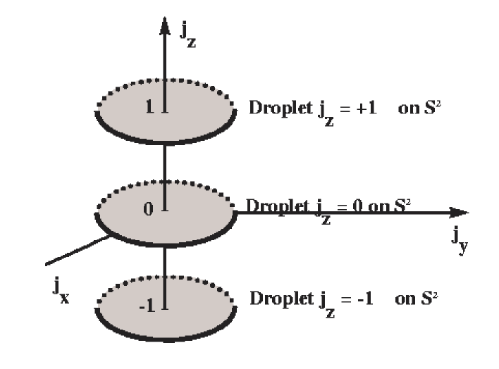
Figure 1: This figure gives a schematic illustration of FQH droplet on $\mathbb{S}^{3}$ with isospin $j=1$; which is constituted of three FQH droplets on $\mathbb{S}^{2}$.

5 Conclusion and outlook

In this paper, we have developed a matrix model proposal for fractional quantum Hall droplets on the spheres $\mathbb{S}^{3}\simeq SU\left(2\right)$ and $\mathbb{S}^{2}\simeq SU\left(2\right)/U_{C}\left(1\right)$. These geometries are realized as hypersurfaces embedded in $\mathbb{C}^{2}\simeq\mathbb{R}^{4}$ and treated as constraint relations implemented in the field action by help of gauge fields. For the case of droplets on $\mathbb{S}^{2}$, this approach may be viewed as an alternative method to the highly non linear matrix model proposal considered recently in [1]. Moreover, the wave function eq(4.36), derived in this paper, completes the results of the above mentioned study. An other powerful point of our proposal is its unified description of both $\mathbb{S}^{3}$ and $\mathbb{S}^{2}$ spheres.

Among the main results obtained in this study, we mention the derivation of a new matrix model proposal for FQH droplets on $\mathbb{S}^{3}$ and its reduction down to $\mathbb{S}^{2}$ by borrowing ideas from gauge constrained systems. After having identified the underlying quantum matrix constraint eqs(4.4-4.5), we have worked out explicitly the droplet ground state solutions for both spheres $\mathbb{S}^{3}$ and $\mathbb{S}^{2}$. We have found that isometries of these manifolds play a central role in building the wave function for ground state of droplets. In particular, we have shown that FQH droplets on $\mathbb{S}^{3}$ carries an isospin $j$ equal to,

$$j=kN\frac{\left(N-1\right)}{2},\qquad l=kl_{1},\qquad l_{1}=\frac{\left(N-1\right)}{2},$$ (5.1)

with $\frac{1}{k}$ being the filling fraction of the Laughlin state. We have also found that a generic droplet on $\mathbb{S}^{3}$ with isospin $j$ and ground state,

$$|\Phi_{k,j}>=\left\{\text{ \ }|\Phi_{k,j,j-p}>,\text{ \ \ }\left|p\right|\leq j\text{ \ }\right\},$$ (5.2)

is made of $\left(2j+1\right)$ droplets on the 2-sphere,

$$|\Phi_{k,j,j-p}>,\qquad p\in\left\{-j,...,j\right\},$$ (5.3)

with fixed value of the relative integer $p$. It would therefore be interesting to construct matrix model for FQH droplets on group manifolds $G$ and cosets $G/H$; then check whether the FQH ground state property relating $\mathbb{S}^{3}\simeq SU\left(2\right)$ and $\mathbb{S}^{2}\simeq SU\left(2\right)/U_{C}\left(1\right)$ is a general feature valid as well for FQH droplets on higher dimensional group manifolds.

In the end of this paper, we would like to add that the next step of our FQH project is to push further this method by applying it to other particular examples. Our immediate interest concerns the derivation of matrix model for wrapped D-string droplets on $K3\simeq T^{\ast}\mathbb{S}^{2}$ and conifold $T^{\ast}\mathbb{S}^{3}$ geometries. This is important for our quest in looking for the connection between FQH droplets on $T^{\ast}\mathbb{S}^{3}$ and the partition function of topological string B model on conifold. Progress in this direction will be reported elsewhere.

Acknowledgement 2

This research work is supported by the program Protars III D12/25, CNRST.

References

- [1] Bogdan Morariu, Alexios P. Polychronakos, Fractional quantum Hall effect on the two-sphere: a matrix model proposal, Phys. Rev. D 72: 125002, 2005, hep-th/0510034
- [2] L. Susskind, The Quantum Hall Fluid and Non-Commutative Chern Simons Theory, hep-th/0101029,
- [3] Simeon Hellerman, Leonard Susskind, Realizing the Quantum Hall System in String Theory, hep-th/0107200
- [4] Alexios P. Polychronakos, Quantum Hall states as matrix Chern-Simons theory, JHEP 0104 (2001) 011, hep-th/0103013.
- [5] A.El Rhalami, E.M. Sahraoui, E.H.Saidi, NC Branes and Hierarchies in Quantum Hall Fluids, JHEP 0205 (2002) 004, hep-th/0108096
- [6] Aziz El Rhalami, El Hassan Saidi, NC Effective Gauge Model for Multilayer FQH States hep-th/0208144, JHEP,
- [7] James Gates Jr, Ahmed Jellal, EL Hassan Saidi, Michael Schreiber, Supersymmetric Embedding of the Quantum Hall Matrix Model, JHEP 0411 (2004) 075 hep-th/0410070
- [8] S.C. Zhang, Quantum Hall effect in higher dimensions, (Talk given at the Conference on Higher Dimensional Quantum Hall Effect, Chern-Simons Theory and Non-Commutative Geometry in Condensed Matter Physics and Field Theory, 1-4/03/2005, AS-ICTP Trieste,
- [9] Dimitra Karabali, Electromagnetic interactions of higher dimensional quantum Hall droplets, Nucl.Phys B726 (2005) 407-420, hep-th/0507027
- [10] Dimitra Karabali, V.P. Nair, Quantum Hall Effect in Higher Dimensions, Nucl.Phys. B641 (2002) 533-546, hep-th/0203264
- [11] V.P. Nair, S. Randjbar-Daemi, Quantum Hall effect on , edge states and fuzzy , Nucl.Phys. B679 (2004) 447-463, hep-th/0309212
-
[12]
EL Hassan Saidi, Topological gauge theory
on conifold and non commutative geometry, Lab/UFR-HEP/0514, GNPHE/0514,
VACBT/0514,
El Hassan Saidi, Moulay Brahim Sedra, Topological string in harmonic space and correlation functions in $S^3$ stringy cosmology, hep-th/0604204, To appear in Nuclear Physics B. - [13] R. Ahl Laamara, L.B Drissi, E H Saidi, D-string fluid in conifold: I. Topological gauge model, Lab/UFR-PHE/0516, Nucl.Phys. B743 (2006) 333-353, hep-th/0604001 .
- [14] R. Ahl Laamara, A. Belhaj, L.B Drissi, E H Saidi, D-string fluid in conifold: III. Matrix model on K3 and conifold, Lab/UFR-PHE/0610, In preparation.
- [15] EL Hassan Saidi, Topological matrix model proposal for Laughlin wave and cousin state, Lab/UFR-HEP0517/GNPHE/0519/VACBT/0519
- [16] Simeon Hellerman, Mark Van Raamsdonk, Quantum Hall Physics = Noncommutative Field Theory, JHEP 0110 (2001) 039, hep-th/0103179