hep-th/0605195

MAD-TH-06-5

Holomorphic Anomaly in Gauge Theories and Matrix Models

Min-xin Huang and Albrecht Klemm

Department of Physics, University of Wisconsin

Madison, WI 53706, U.S.A.

We use the holomorphic anomaly equation to solve the gravitational corrections to Seiberg-Witten theory and a two-cut matrix model, which is related by the Dijkgraaf-Vafa conjecture to the topological $B$-model on a local Calabi-Yau manifold. In both cases we construct propagators that give a recursive solution in the genus modulo a holomorphic ambiguity. In the case of Seiberg-Witten theory the gravitational corrections can be expressed in closed form as quasimodular functions of $\Gamma(2)$. In the matrix model we fix the holomorphic ambiguity up to genus two. The latter result establishes the Dijkgraaf-Vafa conjecture at that genus and yields a new method for solving the matrix model at fixed genus in closed form in terms of generalized hypergeometric functions.

1 Introduction

The holomorphic anomaly equations, discovered in[1] in a world-sheet analysis of a topological twisted $\sigma$-model known as B-model, are a generalisation of Quillens anomaly to higher genus and more general world-sheet theories. Gauge theory are embedded in string theory and in the $N=2$ context the latter can be obtained in double scaling decoupling limit. The holomorphic anomaly equations commute with that decoupling limit and the recursive procedure which determine the higher ${F}^{(g)}(\tau,\bar{\tau})$ [1], which describe certain terms in the coupling to gravity, can be build up entirely from gauge theory quantities. In section 2 the corresponding topological partition of the 4d $N=2$ SUSY gauge is determined by solving the holomorphic anomaly recursively, up to finitely many terms, which have to be fixed by analyzing the boundary behaviour of the ${F}^{(g)}(\tau,\bar{\tau})$. The properties of $F^{(g)}(\tau,\bar{\tau})$ are to a large extend fixed by the modular group of the corresponding Seiberg-Witten curve and we are able to write global expressions them in terms of “almost holomorphic” modular functions of this group. Various holomorphic limits are readily taken from our expressions and provide conjectural solutions to the unitary matrix model [3].

Riemann surfaces $\Sigma_{g}$ of all genus can be embedded in noncompact Calabi-Yau threefolds $X$, i.e. the local limit of the $B$-model exist for an arbitrary Riemann surface. There are choices in this embedding, which affect the reduction of the holomorphic $(3,0)$ form from $X$ to one form $\lambda$ on $\Sigma_{g}$, which is a key datum of the local $B$-model limit. Except for the product case, $\lambda$ will be a meromorphic form with residua and eventually boundary data on open $\Sigma_{g,h}$. In the pure SW-case, there are poles with vanishing residua. In the massive SW-case and other local geometries, one one would have parameters associated with the non-vanishing residua. In section 3 we apply the holomorphic anomaly equations to $N=1$ 4d gauge theory in a geometry proposed by [4]. This is a case where $\lambda$ has essential singularities or differently put one deals with open Riemann surfaces. According to the Dijkgraaf-Vafa correspondence [5] the holomorphic anomaly equations provide here in a particular region solutions to the large $N$ expansion of a complex matrix model, which is the solution to an open string problem. This has a description in the $A$ and the $B$ language as summarized following commuting diagram of duality relations

The Dijkgraaf-Vafa conjecture, relevant to calculate effective terms in $\mathcal{N}=1$ supersymmetric theories in 4d, involves non-compact Calabi-Yau geometries, which are in particular not toric. Explicit test of the conjecture are therefore difficult and have been done only at tree level [5] and at genus one [8, 10]. In the genus one case it is found that the free energy for multi-cut matrix models can be written in closed form [8, 11]. We set the B-model formalism up to get recursively closed expressions at all genus and check the Dijkgraaf-Vafa correspondence of the first non-trivial example, the two cut case, explicitly at genus two.

As in the $N=2$ case, we make a detailed analysis of the moduli space and the modular transformation of the periods in Appendix A, which enables us to solve the theory at various regions in the moduli space. Different from in the $N=2$ case however there is a divisor with essential singularities of the periods in the moduli space, where the perturbative description breaks down. From the topological string point of view we obtain solutions for a new class of non-toric, non-compact Calabi-Yau geometries, which have no point of maximal unipotent monodromy.

2 Gravitational corrections to N=2 Seiberg-Witten Gauge theory

In this section we introduce a B-model, which calculates the higher genus space-time instantons of $N=2$ Seiberg-Witten gauge theory. The genus $g$ generating function ${\cal F}^{(g)}(a)$ of these space-time instantons describe gravitational couplings to the gauge theory [14]. The coefficients of

$$F=\sum_{g=0}^{\infty}\lambda^{2g-2}{\cal F}^{(g)}(a)$$ (2.1)

can be calculated iteratively in the instanton number, $1/a^{4}$ powers below, using localisation in the moduli space of gauge theory [15, 16, 18, 17] or worldsheet instantons [8, 9]. Global properties under the monodromy group, which should be central in the solution of the theory, remain obscure in these approaches. We find that studing the global properties enables us to solve the B-model completly and in particular fix the holomorphic ambiguity. This yields closed modular expressions which determine the instanton contributions to all orders in the instanton number, but are iteratively in the genus i.e. in $\lambda$. We finish the section with some speculations how to obtain closed expressions in $\lambda$ as well.

2.1 Modular properties of the genus zero and genus one sector

We focus on simplest case of $SU(2)$ gauge theory without matter. Generalizations to other gauge groups and matter spectra with asymptotic freedom are certainly possible. The monodromy group of pure $SU(2)$ Seiberg-Witten theory is $\Gamma(2)\in\Gamma_{0}={\rm SL}(2,\mathbb{Z})$ generated by [19]

$$M_{\infty}=PT^{-2},\qquad M_{1}=ST^{2}S\ ,$$ (2.2)

where $S=\left(\begin{array}[]{rr}0&-1\\ 1&0\end{array}\right)$ and $T=\left(\begin{array}[]{rr}1&1\\ 0&1\end{array}\right)$ are the generators of $\Gamma_{0}$ and $P=\left(\begin{array}[]{rr}-1&0\\ 0&-1\end{array}\right)$. Using modular properties as well as the B-model holomorphic anomaly we are able to express the ${\cal F}^{(g)}$ in terms of $\Gamma(2)$ forms and the quasi-modular form of degree two $E_{2}$.

The natural embedding of gauge theory in type IIB string theory [20] is the explanation that the higher genus worldsheet technique of [1] applies to the space-time instanton calculation. More precisely as found in [20] IIB theory on the local Calabi-Yau space ${\cal O}(-2,-2)\rightarrow{\mathbb{P}}^{1}\times{\mathbb{P}}^{1}$ has a double scaling limit in the two complexified Kähler parameters $t_{1},t_{2}$ of ${\mathbb{P}}^{1}\times{\mathbb{P}}^{1}$ in which ${\cal F}^{(g)}(t_{1},t_{2})$ approaches ${\cal F}^{(g)}(a)$. What we find below is that the holomorphic anomaly equation make sense in the limit and can be directly viewed as property of the gauge theory.

The Picard-Fuchs equation for the periods $a=\int_{a}\lambda$ and $a_{D}=\int_{b}\lambda$ of the elliptic curve [19]

$$y^{2}=(x-u)(x-\Lambda^{2})(x+\Lambda^{2})$$ (2.3)

with meromorphic differential $\lambda={\sqrt{2}\over 2\pi}{y\over x^{2}-1}\mathrm{d}x$

$$\frac{\partial^{2}a}{\partial^{2}u}=\frac{a}{4(1-u^{2})}\$$ (2.4)

allows to calculate the genus zero prepotential using the relation ${\partial{\cal F}^{(0)}\over\partial a}=a_{D}$ up an irrelevant constant. Here for convenience we have set the Seiberg-Witten scale $\Lambda=1$, which can be easily recovered by dimensional analysis. The details of the calculation that leads to explicit expressions for the periods can be found in [21]. The elliptic curve (2.3) with $\Gamma(2)$ monodromy has the $j$-function $j(\tau)={(3+u^{2})^{3}\over 27(u^{2}-1)^{2}}$, which allows to write [22]

$$u(\tau)={c+d\over b}\ ,$$ (2.5)

as the Hauptmodul of $\Gamma(2)$ in terms of the ratio $\tau=\int_{b}{\mathrm{d}x\over y}/\int_{a}{\mathrm{d}x\over y}=-\frac{1}{4\pi i}{\partial^{2}{\cal F}^{(0)}\over\partial^{2}a}$ of the periods over the holomorphic one-form. The latter are solution of the ${}_{2}F_{1}$ hypergeometric differential equation $\frac{\partial^{2}a}{\partial^{2}u}=\frac{2u}{(1-u^{2})}\frac{\partial a}{\partial u}+\frac{a}{4(1-u^{2})}$, which implies that the inverse relation to (2.5) can be written in terms of a Schwarz-triangle function (see e.g. [23])

$$\tau(u^{2})=s(\frac{1}{4},\frac{1}{4},1;u^{2}):={i(1-u^{2})^{\frac{1}{4}}\over 2(1-i)}{{}_{2}F_{1}(\frac{1}{4},\frac{1}{4},1;1-u^{2})\over{}_{2}F_{1}(\frac{1}{4},\frac{1}{4},1;\frac{1}{1-u^{2}})}\ .$$ (2.6)

We defined in (2.5) $b=\theta_{2}^{4}$, $c=\theta_{3}^{4}$, $d=\theta_{4}^{4}$ with the relation $b+d=c$. Using the modular transfomation

$$T:\begin{array}[]{rl}b&\rightarrow-b\\ c&\leftrightarrow d\par\end{array}\qquad S:\begin{array}[]{rl}b&\rightarrow-\tau^{2}d\\ d&\rightarrow-\tau^{2}b\\ c&\rightarrow-\tau^{2}c\par\end{array}$$ (2.7)

and (2.2) it is immediate that $u(\tau)$ is invariant under $\Gamma(2)$. For further reference let us note that the discriminant of the elliptic curve is given by $u=\infty$ and

$$\Delta=u^{2}-1=4{cd\over b^{2}}=0\ .$$ (2.8)

The Kähler potential in rigid special geometry is given by (see [24] for a recent review)

$$K=i(X^{I}\bar{F}_{\bar{I}}-{\bar{X}}^{\bar{I}}F_{I})\ .$$ (2.9)

For the Seiberg-Witten curve $X^{1}=a$ and $\tau:={\partial^{2}\over\partial^{2}a}F$ so that the metric becomes

$$g_{a\bar{a}}=\partial_{a}\bar{\partial}_{\bar{a}}K=2\tau_{2}\ .$$ (2.10)

The genus one amplitude is obtained by integrating the genus holomorphic anomaly using the special geometry relation [25]

$$F^{(1)}=-\log(\sqrt{\tau_{2}}\eta\bar{\eta})\ .$$ (2.11)

Note that the holomorphic ambiguity is fixed by requiring that $F^{(1)}$ is invariant under ${\rm SL}(2,{\mathbb{Z}})$ transformations and regular inside the fundamental domain $\cal H$. Indeed $\eta$ is the unique modular form of weight ${1\over 2}$ so that $F^{(1)}$ regular inside $\cal H$.

In the holomorphic limit $\bar{\tau}\rightarrow\infty$, we get [25]

$$\mathcal{F}^{(1)}=-\log(\eta(\tau))=-\frac{1}{2}\log(\frac{\partial a}{\partial u})-\frac{1}{12}\log(u^{2}-1)\ .$$ (2.12)

This agrees with [14]. The form of $\mathcal{F}^{(1)}$ in terms of $u$ and $\frac{\partial a}{\partial u}$ follows in the rigid limit from [25] and was observed in [8]. Using (2.12) and $\eta^{12}=2^{-4}bcd$ one gets

$${\partial a\over\partial u}={\theta_{2}^{2}\over 4}\ .$$ (2.13)

Further with (2.5) and the formulas for the derivatives of the $\theta$ functions we find

$${\cal F}^{(0)}_{,3}(\tau):={\partial^{3}{\cal F}^{(0)}\over\partial^{3}a}=\frac{\partial\tau}{\partial a}={8\sqrt{b}\over cd}={1\over\Delta}\left(\partial u\over\partial a\right)^{3}\ .$$ (2.14)

This can alternatively derived by taking twice the derivative w.r.t. to $a$ in the Matone relation $\mathcal{F}^{(0)}-\frac{1}{2}a\frac{\partial\mathcal{F}^{(0)}}{\partial a}+u=0$ [29]. Using the Picard-Fuchs (2.4) equation and (2.13) we can write the period as

$$a(\tau)={1\over 3\theta_{2}^{2}}(E_{2}+c+d)\ .$$ (2.15)

Closely related expressions for the SW-periods of elliptic curves appear in [14] and for more general gauge groups in [27].

The strong coupling duality element $S:\tau\rightarrow-{1\over\tau}$ of $N=4$ Super-Yang-Mills theory is not trivially realized in pure $N=2$ Seiberg-Witten theory. It relates the gauge instanton expansion in the region of asymptotic freedom ${1\over u},{1\over a}\rightarrow 0$ to the magnetic $U(1)$ which is weakly coupled at the magnetic monopole point $z=(u-1)/2,a_{D}\rightarrow 0$. The gauge coupling of the asymptotic free theory is determined by $\tau(a)$, while the one of the magnetic $U(1)$ is determined by $\tau_{D}(a_{D})$ with the relation

$$\tau_{D}=-{1\over\tau}$$ (2.16)

We note that the one-loop amplitude (2.11) is $S$-duality invariant. The holomorphic limit at the monopole points is taken by $\bar{\tau}_{D}\rightarrow\infty$. Therefore one has

$$\begin{array}[]{rl}\mathcal{F}^{D(1)}(a_{D})=&\displaystyle{-\log(\eta(\tau_{D}))=-\frac{1}{2}\log(\frac{\partial a_{D}}{\partial u})-\frac{1}{12}\log(u^{2}-1)}\\[8.53581pt] =&\displaystyle{\frac{\log(2)}{3}-\frac{i}{6}\,\pi-\frac{\log(\tilde{a}_{D})}{12}-\frac{\tilde{a}_{D}}{2^{5}}-\frac{3\,{\tilde{a}_{D}}^{2}}{2^{9}}-\frac{19\,{\tilde{a}_{D}}^{3}}{2^{12}3}+{O(\tilde{a}_{D})}^{4}}\end{array}$$ (2.17)

We derive, similar as (2.15) was obtained, from the first line of (2.17) a formula for the second period

$$a_{D}(\tau_{D})=-{i\over 3\theta_{4}^{2}}(E_{2}-b-c)\ .$$ (2.18)

This can then be inverted to obtain the series expansion in the second line of (2.17), where we rescale

$$\tilde{a}_{D}:=i{a_{D}\over 2}\ .$$ (2.19)

It is naturally to define an anholomorphic period

$$A(\tau,\bar{\tau})={1\over 3\theta_{2}^{2}}(\hat{E}_{2}(\tau,\bar{\tau})+c+d),$$ (2.20)

with the anholomorphic weight one form

$$\hat{E}_{2}(\tau,\bar{\tau}):=E_{2}(\tau)+{6i\over\pi(\bar{\tau}-\tau)}\ .$$ (2.21)

Different then the Eisenstein series $E_{4}$ and $E_{6}$, holomorphic modular forms of weight $4$ and $6$ which generate the ring of holomorphic forms of $\Gamma_{0}$, the holomorphic $E_{2}$ transforms not quite as modular form of weight $1$, but rather quasi-modular under $\Gamma_{0}$, i.e. with a shift

$$E_{2}\left(a\tau+b\over c\tau+d\right)=(c\tau+d)^{2}E_{2}(\tau)+{12\over 2\pi i}c(c\tau+d)\ .$$ (2.22)

However the anholomorphic piece in (2.20) cancels the shift so that $\hat{E}_{2}(\tau,\bar{\tau})$ transforms as a form of weight $1$.

It follows from (2.20) that $a(\tau)=\lim_{\bar{\tau}\rightarrow\infty}A(\tau,\bar{\tau})$ and $a_{D}(\tau_{D})=\lim_{\bar{\tau}_{D}\rightarrow\infty}\frac{1}{\tau_{D}}A(-{1\over\tau_{D}},-{1\over\bar{\tau}_{D}})$. Morover S-duality transformations (2.7) allow us to write $a$ and $a_{D}$ as functions of $\tau$ or $\tau_{D}$. In particular we can integrate (2.15) w.r.t. $a_{D}$ in the magnetic phase

$${\cal F}^{D(0)}=\frac{1}{2}{\tilde{a}_{D}}^{2}\log\left(-{\tilde{a}_{D}\over 2}\right)+4\tilde{a}_{D}-\frac{{3\tilde{a}_{D}}^{2}}{2^{2}}+\frac{{\tilde{a}_{D}}^{3}}{2^{4}}+\frac{5\,{\tilde{a}_{D}}^{4}}{2^{9}}+\frac{11\,{\tilde{a}_{D}}^{5}}{2^{12}}+O(\tilde{a}_{D}^{6})\ .$$ (2.23)

2.2 Propagators and integrating the holomorphic anomaly equations

From the genus zero and genus one amplitude one can derive the propagator [1]. With the simplification for local $B$-model explained in [26] we obtain

$$S^{aa}=S={2{F}^{(1)}_{,1}\over{F}^{(0)}_{,3}}={1\over 24}\left(E_{2}(\tau)-{3\over\pi\tau_{2}}\right)=:{1\over 24}\hat{E}_{2}(\tau,\bar{\tau})\ ,$$ (2.24)

which in the holomorphic limit becomes

$${\cal S}^{aa}={\cal S}={2{\cal F}^{(1)}_{,1}\over{\cal F}^{(0)}_{,3}}={1\over 24}E_{2}(\tau)\ .$$ (2.25)

This quantity contains the contribution from the boundaries of the WS moduli space in the topological string theory. It is closely related to $T_{k,l}$ the quantity that arises if one considers correlators of integrated two-form operators constructed from the descent equation in the gauge theory on four manifolds. More precisely intersections of the correponding 2-cycles require contact terms which are $T_{k,l}=S^{a_{i}a_{j}}{\partial u_{k}\over\partial a_{i}}{\partial u_{l}\over\partial a_{j}}$, see [28].

Equations (2.14,2.11,2.24) define the data needed to recursively solve the $B$-model [1]. Using the fact that the formalism of integrating the holomorphic anomaly equations commutes with the double scaling limit taken to obatin the gauge theory [20] and power counting in the propagator in the Feynmann rules of [1] we obtain the following general result

$$F^{(g)}(\tau,\bar{\tau})=X^{g-1}\sum_{k=0}^{3(g-1)}\hat{E}_{2}^{k}(\tau,\bar{\tau})c^{(g)}_{k}(\tau)\ .$$ (2.26)

Here we defined $X={b\over 1728c^{2}d^{2}}={1\over{108(u^{2}-1)^{2}b^{3}}}$, which transforms as a weight $-3$ object $X({a\tau+b\over c\tau+d})\rightarrow{1\over(c\tau+d)^{6}}X(\tau)$ under $\Gamma(2)$. $F^{(g)}$ is invariant under $\Gamma(2)$, which implies that $c^{(g)}_{k}$ are homogeneous of weight $3(g-1)-k$ in $(b,c,d)$. Further conditions on $c^{(g)}_{k}$ come from regularity at $u=0$ and a gap condition at the conifold $u=1$ as dicussed below.

We obtain the holomorphic limits of the expansion in the asymptotic freedom and the strong coupling region as

$${\cal F}^{(g)}(a)=\lim_{\bar{\tau}\rightarrow\infty}F^{(g)}(\tau,\bar{\tau}),\quad{\rm and}\quad{\cal F}^{D(g)}(a_{D})=\lim_{\bar{\tau}_{D}\rightarrow\infty}F^{(g)}(-{1\over\tau_{D}},-{1\over\bar{\tau}_{D}})\$$ (2.27)

and the $a$ or $a_{D}$ ($\tilde{a}_{D}$) expansion are obtained by inverting (2.15) or (2.18). We note that the leading behaviour of electric and magnetic expansion in these parameters is

$${\cal F}^{(g)}(a)\sim{(-1)^{g}B_{2g}\over g(2g-2)(2a)^{2g-2}}\quad{\rm and}\quad{\cal F}^{D(g)}(a_{D})\sim{B_{2g}\over 2g(2g-2){\tilde{a}_{D}}^{2g-2}}\$$ (2.28)

respectively. The first asymptotic behaviour can be derived in the gauge theory limit of type II theory on ${\cal O}(-2,-2)\rightarrow{\mathbb{P}}^{1}\times{\mathbb{P}}^{1}$. More precisley one uses in the Gopakumar-Vafa expansion $\frac{1}{\left(2\sin{m\lambda\over 2}\right)^{2}}=\sum_{g=0}\lambda^{2g-2}(-1)^{(g-1)}\frac{B_{2g}}{2g(2g-2)!}m^{2g-2}$ and the multiplicity $n^{(g)}_{m,0}=\delta_{g,0}\delta_{m,0}=-2$ of BPS states corresponding to constant maps on one ${\mathbb{P}}^{1}$ as well as properties of the limit discussed in [20]. The derivation is similar as for the constant map contribution $\int_{\overline{{\cal M}_{g}}}c^{3}_{g-1}=\frac{|B_{2g}B_{2g-2}|}{2g(2g-2)(2g-2)!}$ in [38]. The asymptotic in the magnetic expansion comes from the occurrence of the $c=1$ string at the conifold [40].

We come now to the explicite iterative solutions in the genus. For example the recursive definition of $F^{(2)}$ is

$${F}^{(2)}(\tau,\bar{\tau})={1\over 2}S{F}^{(1)}_{,2}+{1\over 2}S({F}^{(1)}_{,1})^{2}+{5\over 24}S^{3}({F}^{(0)}_{,3})^{2}-{1\over 8}S^{2}{F}^{(0)}_{,4}-{1\over 2}S^{2}{F}^{(1)}_{,1}{F}^{(0)}_{,3}+Xc^{(2)}_{0}(u)\ ,$$ (2.29)

were $c^{(2)}_{0}(u)$ is the holomorphic ambiguity at genus two. This ambiguity must be invariant under $\Gamma(2)$, which implies that it can be written in terms of $u$. Moreover regularity of $F^{(g)}$ at $u\rightarrow\infty$ and the leading pole behaviour at $u\rightarrow 1$ implies that it is of the form

$$X^{g-1}c^{(g)}_{0}(u)=u^{3-g}\sum_{i=1}^{2g-2}{A^{(g)}_{i}\over\Delta^{i}(u)}\ .$$ (2.30)

Note that $A^{(g)}_{i}$ are undetermined constants and the right hand is a rational function of the $\Gamma(2)$ invariant function $u$. Using (2.14,2.11) and the standard formulas for the derivatives of $\theta_{i},E_{2}$ we may write (2.29) with $h=(b+2d)$ as

$${F}^{(2)}(\tau,\bar{\tau})={X\over 3}\left(5\hat{E}_{2}^{3}-9\hat{E}_{2}^{2}h+6\hat{E}_{2}(b^{2}+cd)-{h(16b^{2}+19cd)\over 10}\right)\ ,$$ (2.31)

an almost holomorphic modular function of $\Gamma(2)$. Here we determined the ambiguity as follows. Using (2.27,2.15) we can expand (2.31) in the electric and magnetic holomorphic limits. With the leading behaviour (2.28) we found $A^{(2)}_{1}=-{19\over 12960}$ and $A^{(2)}_{2}=-{2\over 405}$. This yields

$${\cal F}^{(2)}=-\frac{1}{240\cdot 2\,a^{2}}-\frac{11}{2^{18}\,a^{10}}-\frac{117}{2^{22}\,a^{14}}-\frac{171201}{2^{34}\,a^{18}}+O({1\over a^{22}})$$ (2.32)

This series predicts all genus 2 instantons and checks with the coefficients that appear in the literature [15][8]. The expansion in $a_{D}$ is obtained from (2.31) using (2.27,2.7,2.18)

$${\cal F}^{D(2)}=-\frac{1}{240\,{\tilde{a}_{D}}^{2}}-\frac{\tilde{a}_{D}}{2^{13}}-\frac{13\,{\tilde{a}_{D}}^{2}}{2^{16}}-\frac{129\,{\tilde{a}_{D}}^{3}}{2^{17}5}+\ {O({\tilde{a}_{D}}^{4})}$$ (2.33)

Solving the recursion for genus 3 yields [26]

$$\begin{array}[]{rl}{F}^{(3)}=&S{F}^{(2)}_{,1}{F}^{(1)}_{,1}-{1\over 2}S^{2}{F}^{(2)}_{,1}{F}^{(0)}_{,3}+{1\over 2}S{F}^{(2)}_{,2}+{1\over 6}S^{3}({F}^{(1)}_{,1})^{3}{F}^{(0)}_{,3}-{1\over 2}S^{2}{F}^{(1)}_{,2}({F}^{(1)}_{,1})^{2}\cr&-{1\over 2}S^{4}({F}^{(1)}_{,1})^{2}({F}^{(0)}_{,3})^{2}+{1\over 4}S^{3}({F}^{(1)}_{,1})^{2}{F}^{(0)}_{,4}+S_{2}^{3}{F}^{(1)}_{,2}{F}^{(1)}_{,1}{F}^{(0)}_{,3}-{1\over 2}S^{2}{F}^{(1)}_{,3}{F}^{(1)}_{,1}\cr&-{1\over 4}S^{2}({F}^{(1)}_{,2})^{2}+{5\over 8}S^{5}{F}^{(1)}_{,1}({F}^{(0)}_{,3})^{3}-{2\over 3}S^{4}{F}^{(1)}_{,1}{F}^{(0)}_{,4}{F}^{(0)}_{,3}-{5\over 8}S^{4}{F}^{(1)}_{,2}({F}^{(0)}_{,3})^{2}\cr&+{1\over 4}S^{3}{F}^{(1)}_{,2}{F}^{(0)}_{,4}+{5\over 12}S^{3}{F}^{(1)}_{,3}{F}^{(0)}_{,3}+{1\over 8}S^{3}{F}^{(0)}_{,5}{F}^{(1)}_{,1}-{1\over 8}S^{2}{F}^{(1)}_{,4}-{7\over 48}S^{4}{F}^{(0)}_{,5}{F}^{(0)}_{,3}\cr&+{25\over 48}S^{5}{F}^{(0)}_{,4}({F}^{(0)}_{,3})^{2}-{5\over 16}S^{6}({F}^{(0)}_{,3})^{4}-{1\over 12}S^{4}({F}^{(0)}_{,4})^{2}+{1\over 48}S^{3}{F}^{(0)}_{,6}+X^{2}c^{(3)}_{0}(u)\ ,\end{array}$$ (2.34)

and we determined the coefficients $A^{(3)}_{1}=\frac{59}{2449440}$, $A^{(3)}_{2}=\frac{14669}{3265920}$, $A^{(3)}_{3}=\frac{4133}{204120}$ and $A^{(3)}_{4}=\frac{5359}{306180}$. This yields the following almost complex modular expression for ${F}^{(3)}$

$$\begin{array}[]{rl}{F}^{(3)}=&{4X^{2}}\biggl{(}5\hat{E}_{2}^{6}-25\hat{E}_{2}^{5}h+40\hat{E}_{2}^{4}(2b^{2}+5cd)-{1\over 3}\hat{E}_{2}^{3}h(529b^{2}+559cd)+\cr&{\hat{E}_{2}^{2}\over 5}(1172b^{4}+4060b^{2}cd+1223(cd)^{2})-\hat{E_{2}\over 5}h(844b^{4}+1685b^{2}cd+310(cd)^{2})+\cr&{1\over 210}(10718b^{6}+49596b^{4}cd+44007b^{2}(cd)^{2}+944(cd)^{3})\Biggr{)}\ ,\end{array}$$ (2.35)

from which the electric

$${\cal F}^{(3)}=\frac{1}{1008\cdot 2^{3}}\left(-\frac{1}{a^{4}}+\frac{441}{2^{12}a^{12}}+\frac{18459}{2^{16}a^{16}}+\frac{62106849}{2^{28}a^{20}}+\frac{256368735}{2^{31}a^{24}}+O(\frac{1}{a^{28}})\right)$$ (2.36)

and magnetic expansions

$${\cal F}^{D(3)}=\frac{1}{1008}\frac{1}{{\tilde{a}_{D}}^{4}}-\frac{9\,\tilde{a}_{D}}{2^{20}}-\frac{143\,{\tilde{a}_{D}}^{2}}{2^{22}}-\frac{63827\,{\tilde{a}_{D}}^{3}}{2^{27}7}+{O({\tilde{a}_{D}}^{4})}$$ (2.37)

follow from (2.27). The number of terms in the modular expressions of $F^{(g)}$ grow much slower then the number of graphs in the holomorphic anomaly equation, because many graph contributions are proportional to the same quasimodular form. For genus four, where the holomorphic anomaly equation has 83 graphs we find

$${F}^{(4)} = 4X^{3}\big{\{}\frac{1150}{9}\hat{E}_{2}^{9}-985\hat{E}_{2}^{8}h+2\hat{E}_{2}^{7}(2399b^{2}+7001cd)$$ (2.38)

$$-\frac{14}{3}\hat{E}_{2}^{6}h(3761b^{2}+6125cd)+\frac{3}{5}\hat{E}_{2}^{5}(85863b^{4}+363344b^{2}cd+240083(cd)^{2})$$

$$-\frac{1}{5}\hat{E}_{2}^{4}h(604469b^{4}+1677340b^{2}cd+547811(cd)^{2})$$

$$+\frac{2}{5}\hat{E}_{2}^{3}(531266b^{6}+2793615b^{4}cd+3285123b^{2}c^{2}d^{2}+447656(cd)^{3}))$$

$$-\frac{2}{35}\hat{E}_{2}^{2}h(4430756b^{6}+16550337b^{4}cd+11925927b^{2}(cd)^{2}+889964(cd)^{3})$$

$$+\frac{1}{175}\hat{E}_{2}(31232428b^{8}+195274840b^{6}cd+329613819b^{4}(cd)^{2}+130729960b^{2}(cd)^{3}$$

$$+3566728(cd)^{4})-\frac{1}{1575}h(87826748b^{8}+423770948b^{6}cd$$

$$+511313601b^{4}(cd)^{2}+128098172b^{2}(cd)^{3}+4442006(cd)^{4})\big{\}}$$

with electric

$${\cal F}^{(4)}=\frac{-}{1}{1440\cdot 2^{5}}\left(\frac{1}{a^{6}}+\frac{765}{2^{12}a^{14}}+\frac{126195}{2^{16}a^{18}}+\frac{1925006715}{2^{29}a^{22}}+\frac{14420664765}{2^{32}a^{26}}+{\cal O}(\frac{1}{a^{30}})\right)$$ (2.39)

and magnetic expansion

$${\cal F}^{D(4)}=-\frac{1}{1440{\tilde{a}_{D}}^{6}}+\frac{1125\ {\tilde{a}_{D}}}{2^{29}}-\frac{3915\,{\tilde{a}_{D}}^{2}}{2^{28}}+\frac{4786021\,{\tilde{a}_{D}}^{3}}{2^{35}}+{O({\tilde{a}_{D}}^{4})}$$ (2.40)

We derived expressions for $F^{(g)}$ in terms of modular forms up to genus six and checked the large $a$ expansions against results made available to us by Nakajima. Let us report here the dual expansions, which are interesting as they correspond to perturbations of the $c=1$ string at the selfdual radius by momentum operators

$${\cal F}^{D(5)}=\frac{1}{1056\,{\tilde{a}_{D}}^{8}}-\frac{77175\,{\tilde{a}_{D}}}{2^{36}}-\frac{100971\,{\tilde{a}_{D}}^{2}}{2^{32}}-\frac{5142558213\,{\tilde{a}_{D}}^{3}}{2^{43}11}+{O({\tilde{a}_{D}^{4}})}\ ,$$ (2.41)

$${\cal F}^{D(6)}=-\frac{691}{327600\,{\tilde{a}_{D}}^{10}}-\frac{18753525{\tilde{a}_{D}}}{2^{44}}-\frac{16908525{\tilde{a}_{D}}^{2}}{2^{40}}-\frac{672990085791{\tilde{a}_{D}}^{3}}{2^{49}13}+{O({\tilde{a}_{D}^{4}})}\ .$$ (2.42)

2.3 Fixing the ambiguity

In (2.26) all $c^{(g)}_{k}$ except for $c^{(g)}_{0}$, the holomorphic ambiguity, are determined by the recursion relations (2.29,2.34) that follow from the holomorphic anomaly equation in terms of lower genus $F^{(g)}$. Genrally fixing the holomorphic ambiguity is a major problem in the B-model, which however the case at hand is completly solvable. The discriminant locus of the curve (2.3) is at $u=\infty$ and at $u=\pm 1$ where (2.3) develops a node. At all other points in the moduli space of the Seiberg-Witten geometry $F^{(g)}$ must be regular. As follows from the global properties of the $\theta$ functions and $E_{2}$, regularity at $u=0$ restricts the form of $c^{(g)}_{k}(\tau)$ to

$$c^{(g)}_{k}=h^{(1+(-1)^{g+k})\over 2}P_{d(g,k)}(b^{2},cd),$$ (2.43)

where $P_{d(g,k)}(b^{2},cd)$ is an homogeneous polynomial in $b,c,d$ of degree

$$d(g,k)=3(g-1)-k-{(1+(-1)^{g+k})\over 2}\ ,$$ (2.44)

with ${d(g,k)\over 2}+1$ coefficients. In particular in the ambiguity $c^{(g)}_{0}$ the number of unknown coefficients of this polynomial grows with $\sim{3\over 2}g$ slower then the number of the $A_{i}^{(g)}$ in (2.30), which grows with $\sim 2g$.

Moreover the leading terms in (2.33,2.37,2.40,2.41,2.42) correspond to correlators of the cosmological constant operator of the $c=1$ matrix model in the genus g vacuum sector [40]. Very important is the occurence of the gap in ${\cal F}^{(g)D}$, i.e. the absence of terms $\frac{1}{{\tilde{a}_{D}}^{k}}$, $k=0,\ldots,2g-3$. The $2g-2$ gap conditions fix the $A^{(g)}_{i}$, $i=1,\ldots,2g-2$ constants and hence the ambiguity (2.30). Together with the anomaly equation this provides a very efficient way to solve the theory completly. The asymptotic (2.28) and the particular form of (2.43) are further consistency constraints confirming the gap property. A gap follows if there is a matrix model ${1\over N}$ expansion for the holomorphic topological string at a critical point, as e.g. at the orbifold point in the local ${\cal O}(-2,-2)\rightarrow{\mathbb{P}}^{1}\times{\mathbb{P}}^{1}$ model discussed [7]. In this case the measure integration yields at each genus the negative power term in expansion parameter and the perturbative terms start with positive powers. This particular behaviour of the magnetic expansion of the N=2 pure SU(2) model at the conifold is hence explainable by the proposed unitary matrix model [3]. As we saw above the model is solved by the gap property and the holomorphic anomaly. If one would like to employ ${1\over N}$ techniques in order to determine the weak coupling instanton expansion one would have to do exactly what we have done in (2.26) namely to write the result globally. More generally the gap can be understood from the absence of correlators of the ground ring operators [30] in the $c=1$ string describing the limit of the toplogical string near the nodal singularity (conifolds) of local models. Indeed we have checked that the gap occurs also at the conifold in the local ${\cal O}(-3)\rightarrow{\mathbb{P}}^{2}$ geometry and fixes the ambiguity of this model. How this extends generally to singularities of local models and the modifications for singularities of global models will be discussed in [51].

If we absorb $X$ into genus expansion parameter $\lambda$ in (2.26), it becomes a sum of a quasi-modular form. The simplest example of such an expansion, where the coefficients are however modular forms of the full modular group $\Gamma_{0}$ appears in Hurwitz theory on $T^{2}$ [32]. As reviewed there this leads directly to combinatorial problem that is solved by free fermions and $Z=e^{F}$ can be written in a product form that has been recognized as a generalized $\theta$-function product form in [33]. More examples of such product forms are provided by vertex algebras [34, 35] and arise in heterotic type II duality [36, 37, 38, 39]. It would be interesting to see whether the SW partition function is related to a generalized $\Gamma(2)$ theta function.

3 Dijkgraaf-Vafa conjecture

In [5], Dijkgraaf and Vafa proposed a remarkable relation between B-model topological string on a non-compact Calabi-Yau geometry and a matrix model.

3.1 Dijkgraaf-Vafa transition and geometric engineering

The $n$ cut matrix model is obtained by reducing holomorphic Chern-Simons theory on D5-branes wrapping $n$ ${\mathbb{P}}^{1}$’s in a modification of the geometry ${\cal O}(-2)\oplus{\cal O}(0)\rightarrow{\mathbb{P}}^{1}$. The k-th ${\mathbb{P}}^{1}$ is wrapped by $N_{k}$ branes, $k=1,\ldots,n$. In the modified geometry the location of the ${\mathbb{P}}^{1}$’s in the originally flat ${\cal O}(0)$ $x$-direction is now fixed at the minima of a potential $W(x)$ of degree $n+1$. E.g. the $n=1$ geometry is the blown up conifold ${\cal O}(-1)\oplus{\cal O}(-1)\rightarrow{\mathbb{P}}^{1}$. The reduction yields a complex bosonic matrix model with the matrix potential $W^{\prime}(x)$, that needs as additional data the choice of contour for the eigenvalue integration [5].

The B-model geometry emerges after a transitions in which the $n$ ${\mathbb{P}}^{1}$’s are shrunken and deformed to $S^{3}$’s. It has a local description as a hypersurface in $\mathbb{C}^{4}$

$$vw=W^{\prime}(x)^{2}+f(x)+y^{2}$$ (3.45)

where $x,y,v,w$ are coordinates of $\mathbb{C}^{4}$, $f(x)$ is polynomial of degree $n-1$ that splits the $n$ double zeros of $W^{\prime}(x)^{2}$.

The latter geometry has been considered in [4] to geometrically engineer ${\cal N}=1$ four-dimensional supersymmetric gauge theory. After the transition the breaking to ${\cal N}=1$ is achieved by putting $N_{k}$ units of Ramond flux on the $S^{3}$’s and the topological string or the matrix model calculates terms in the ${\cal N}=1$ effective gauge theory. In [5] it is already shown that the special geometry relation that determine the tree level (genus zero) topological string amplitude $F^{(0)}$ on the geometry (3.45) arise from the planar diagrams of the corresponding matrix model. The planar loop equation of the matrix model gives the spectral curve of the local geometry and the effective superpotential in a large class of $\mathcal{N}=1$ gauge theory can be computed exactly by the genus zero amplitude of matrix model or topological string. It is conjectured that higher genus topological B-model string amplitudes should also be computed by higher genus diagrams in the matrix model.

The meaning of the topological string amplitudes $F^{(g>0)}(S_{i})$ in the effective theory is as follows. In $\mathcal{N}=2$ supergravity action they determine the exact moduli dependence of the $F$-terms

$$\int d^{4}x\int d^{4}\theta F^{(g)}(S_{i})(\mathcal{W}^{\alpha\beta}\mathcal{W}_{\alpha\beta})^{g}$$ (3.46)

here $\mathcal{W}_{\alpha\beta}$ is the $\mathcal{N}=2$ graviphoton superfield and the $S_{i}$ are the $\mathcal{N}=2$ vector multiplets whose complex scalar field corresponds to the moduli of Calabi-Yau manifold. After integrating over the $\mathcal{N}=2$ superspace these terms become the coupling $R_{+}^{2}F^{2g-2}_{+}$ of the self-dual part of the Ricci tensor $R_{+}$ to the selfdual part of the graviphoton field strength $F_{+}$.

After breaking of $\mathcal{N}=2$ to $\mathcal{N}=1$ by fluxes the topological string amplitudes $F^{(g>0)}(S_{i})$ occur in the following two terms of the $\mathcal{N}=1$ action [41, 42, 43]

$$\Gamma_{1}=g\int d^{4}x\int d^{2}\theta\mathcal{W}_{\alpha\beta\gamma}\mathcal{W}^{\alpha\beta\gamma}(F_{\delta\xi}F^{\delta\xi})^{g-1}F^{(g)}(S_{i}),$$ (3.47)

$$\Gamma_{2}=\int d^{4}x\int d^{2}\theta(F_{\alpha\beta}F^{\alpha\beta})^{g}N_{i}\frac{\partial F^{(g)}(S_{i})}{\partial S_{i}}\ .$$ (3.48)

Here $\mathcal{W}_{\alpha\beta\gamma}$ are now $\mathcal{N}=1$ gravitino multiplet, and $S_{i}$ are the $\mathcal{N}=1$ glueball chiral superfields coming from the original $\mathcal{N}=2$ vector multiplets [41]. The graviphoton field $F_{\alpha\beta}$ can be treated as background field in the $\mathcal{N}=1$ theory. In [41] a C-deformation is introduced to deform the anti-commutation relation of gluino $\psi_{\alpha}$ to the followings

$$\{\psi_{\alpha},\psi_{\beta}\}=2F_{\alpha\beta}$$ (3.49)

It is shown that the effect of turning on the graviphoton background $F_{\alpha\beta}$ can be captured by this C-deformation, and the $F^{(g)}$ in the second contribution $\Gamma_{2}$ (3.48) are computed by matrix models at genus $g$. We can also see that the first term $\Gamma_{1}$ in (3.47) contributes at genus $g=1$ even there is no graviphoton background $F_{\alpha\beta}$. It is shown in [42] that this genus one contribution is also computed by matrix model genus one diagrams. There are also some other types of gravitational corrections besides (3.47,3.48) of the form $W_{\alpha\beta\gamma}W^{\alpha\beta\gamma}S^{n}$ from planar diagrams, which become trivial after the extremization of the glue ball superfield $S$ [43]. Our results confirm these very interesting ideas in [41, 42, 43] by a first direct tests of the connection between topological strings and matrix models at higher genus without using the superspace techniques in the effective gauge theory.

3.2 The two cut geometry and the tree level and genus one amplitudes

We consider now the case of a cubic potential $W(x)=\frac{m}{2}x^{2}+\frac{g}{3}x^{3}$ in the Dijkgraaf-Vafa geometry (3.45). The degree one polynomial $f(x)=\mu_{1}x+\mu_{0}$ splits the double zeros of $W^{\prime}(x)^{2}$ at $x=a_{1}$ and $x=a_{2}$ to the four roots $a_{1}^{\pm},a_{2}^{\pm}$ of the equation

$$W^{\prime}(x)^{2}+f(x)=0$$ (3.50)

We adopt the notation of [8, 4], and change variable $(a_{1}^{-},a_{1}^{+},a_{2}^{-},a_{2}^{+})\equiv(x_{1},x_{2},x_{3},x_{4})\rightarrow(z_{1},z_{2},Q,I)$ where

$$z_{1}\equiv\frac{1}{4}(x_{2}-x_{1})^{2},~{}~{}~{}~{}z_{2}\equiv\frac{1}{4}(x_{4}-x_{3})^{2}$$

$$Q\equiv\frac{1}{2}(x_{1}+x_{2}+x_{3}+x_{4})=-\frac{m}{g}$$

$$I\equiv\frac{1}{4}[(x_{3}+x_{4})-(x_{1}+x_{2})]^{2}=\left({m\over g}\right)^{2}-2(z_{1}-z_{2})\ .$$ (3.51)

The local Calabi-Yau geometry (3.50) depends really only two complex structure deformations. We will use $(z_{1},z_{2})$ or below the A-periods $S_{1}$ and $S_{2}$ to parameterize them. The dependence of the genus zero super- and the higher genus potentials $F^{(g)}$ can be reconstructed from scaling laws and dimensional considerations. In particular we frequently set $g,m=1$.

The fundamental periods of the local geometry are

$$S_{i}=\frac{1}{2\pi i}\int_{a_{i}^{-}}^{a_{i}^{+}}\lambda,\qquad\Pi_{i}=\frac{1}{2\pi i}\int_{a_{i}^{+}}^{\Lambda}\lambda\ ,$$

where $i=1,2$ and $\lambda=dx\sqrt{W^{\prime}(x)^{2}+f(x)}$ is a meromorphic differential which emerges after integrating the holomorphic Calabi-Yau (3,0)-form over an $S^{2}$ fibre direction of the ${S^{3}}^{\prime}$s in (3.45) [4]. In [4] the integrals where further calculated perturbatively for small $z_{i}$. This limit corresponds to vanishing ${S^{3}}^{\prime}s$ and is suitable for the perturbative matrix model expansion. Solving the B-model and fixing its ambiguity requires a global understanding of the complex moduli space in $(z_{1},z_{2})$. We therefore derive the Picard-Fuchs equations and use them to explore the global properties of the integrals $S_{i}$ and $\Pi_{i}$.

We find that derivatives of $\lambda$ w.r.t. $z_{i}$ up to second order multiplied with suitable polynomials in $z_{i}$ combine to a total derivative, i.e. ${\cal L}_{i}\lambda=\sum_{k+l\leq 2}p^{(k,l)}({\underline{z}})\partial^{k}_{z_{1}}\partial^{l}_{z_{2}}\lambda=\mathrm{d}g_{i}(x,z_{1},z_{2})$. Naively the differential ideal with this property is generated by three independent differential operators ${\cal L}_{i}$. However $\mathrm{d}g_{i}(x,z_{1},z_{2})$ is a meromorphic differential with non-vanishing residua, hence one cannot conclude from the exactness that ${\cal L}_{i}\int_{\Gamma}\lambda=0$. For the following two operators the residua vanish

$$\begin{array}[]{rl}{\cal L}_{1}=&\displaystyle{2z_{1}(2z_{1}+6z_{2}-1)\partial_{z_{1}}^{2}+(1-10z_{1}+12{z_{1}}^{2}+4z_{1}z_{2})\partial_{z_{1}}\partial_{z_{2}}+(3-2z_{1}-6z_{2})\partial_{z_{1}}}\\ &+(1\leftrightarrow 2)\\[8.53581pt] {\cal L}_{2}=&\displaystyle{(2z_{1}+2z_{2}-1)[-2z_{1}(1-4(z_{1}+z_{2})+5{z_{1}}^{2}-2z_{1}z_{2}-3{z_{2}}^{2})\partial_{z_{1}}^{2}+(z_{1}+z_{2})}\\ &\displaystyle{(1-8z_{1}+6{z_{1}}^{2}-6z_{1}z_{2})\partial_{z_{1}}\partial_{z_{2}}]+(z_{1}(7-18z_{2}+26{z_{2}}^{2}+46{z_{1}}^{2}+{z_{1}}(62z_{2}-39))}\\ &\displaystyle{-3z_{2}(1-3z_{2}+2z_{2}^{2})))\partial_{z_{1}}-3(1-12z_{1}+18{z_{1}}^{2}+14z_{1}z_{2})+(1\leftrightarrow 2)\ .}\end{array}$$ (3.52)

These Picard-Fuchs operators annihilate the periods and fix their expansion up to linear combinations. The discriminant of these differential operators has the following components

$$\begin{array}[]{rl}C_{1}:&z_{1}=0,\quad C_{2}:\ z_{2}=0,\quad I:\ I=1-2z_{1}-2z_{2}=0,\\[5.69054pt] J:&J=(x_{1}-x_{2})(x_{2}-x_{3})(x_{2}-x_{4})(x_{1}-x_{4})\\[5.69054pt] &\phantom{J}=(1-3z_{1})^{2}-6z_{2}+9z_{2}^{2}+14z_{1}z_{2}=0,\end{array}$$ (3.53)

whose schematic intersection after a suitable desingularisation of three order tangencies is depicted in Fig. 1.

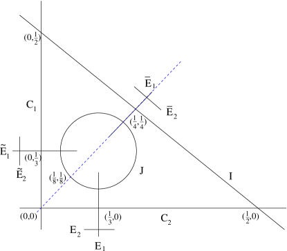
Figure 1: Divisors in the moduli space of B-model, $(z_{1},z_{2})=(0,0)$ is the matrix model expansion point and along the dash line one has enhanced $N=2$ SUSY.

According to the Dijkgraaf-Vafa correspondence the periods $S_{i}$ are identified with the filling fractions $N_{i}$, with $\sum_{i=1}^{n}N_{i}=N$, of eigenvalues in the large $N$ limit of the dual matrix model, and it is shown that the special geometry relation and Picard-Fuchs equations are reproduced in the planar limit of the matrix model [5] and the genus zero topological string amplitude $F^{(0)}$ follows from integrating the special geometry relation ${\partial F^{(0)}\over\partial S_{i}}=\Pi_{i}$. To analyze the exact effective superpotential $W_{eff}=2\pi i\sum_{i}(N_{i}\Pi_{i}+\alpha_{i}S_{i})$, where $N_{i}$ and $\alpha_{i}$ are 3-form flux quanta through the $A_{i}$ and $B_{i}$ cycles respectively, globally we need to the periods troughout the complex moduli space. This is done in appendix A, where we also find that there is no point where the periods degenerate quadratically in the logarithms.Which is the signal of a large volume or maximal unipotent point in the moduli space.

Also at one loop the conjecture holds [8, 10]. The B-model expression for the one loop free energy $F^{(1)}$ obtained by integrating (4.59) using (4.58) and fixing integration constants it turns out to be [8]

$$F^{(1)}={1\over 2}\log\left({\rm det}\left(\partial z_{i}\over\partial S_{j}\right)(z_{1}z_{2})^{-{1\over 6}}IJ^{2\over 3}\right)\ ,$$ (3.54)

where we obtain the periods $S_{i}$ in terms of complex structure moduli $z_{i}$ and the corresponding inverse series

$$S_{1}(z_{1},z_{2},g)=\frac{1}{4}z_{1}-\frac{g^{2}}{8}z_{1}(2z_{1}+3z_{2})-\frac{g^{4}}{32}z_{1}(4z_{1}^{2}+13z_{1}z_{2}+9z_{2}^{2})+\mathcal{O}(g^{6})$$

$$S_{2}(z_{1},z_{2},g)=-S_{1}(z_{2},z_{1},g)$$

$$z_{1}(S_{1},S_{2},g)=4S_{1}+8g^{2}S_{1}(2S_{1}-3S_{2})+8g^{4}(20S_{1}^{2}-67S_{1}S_{2}+39S_{2}^{2})+\mathcal{O}(g^{6})$$

$$z_{2}(S_{1},S_{2},g)=z_{1}(-S_{2},-S_{1},g)$$ (3.55)

from the two power series solutions to (3.52) at $(z_{1},z_{2})=(0,0)$. Identifying $S_{i}$ with the filling fractions $N_{i}$ we get the genus one contributions to (B.121). Note that the integration constants $c_{i}$ in $(z_{1}z_{2})^{c_{1}}I^{c_{2}}J^{c_{3}}$, which fix the behaviour of $F^{(1)}$ at the discriminant components are global data do not depend on the base point $(z_{1},z_{2})=(0,0)$ or the holomorphic limit $\bar{S}_{\bar{\imath}}\rightarrow 0$ taken at this base point to obtain the matrix model expansion. The coefficient $c_{1}=-{1\over 6}$ at the conifold (shrinking $S^{3}$) is a universal property of the topological B-model.

To solve the B-model recursion we need the genus zero three point functions, which are rational functions in complex structure moduli.

$$C_{z_{1}z_{1}z_{1}}=\frac{1-(6z_{1}+5z_{2})g^{2}+3(3z_{1}^{2}+3z_{1}z_{2}+2z_{2}^{2})g^{4}}{16g^{4}z_{1}I^{2}},\quad C_{z_{1}z_{1}z_{2}}=\frac{1-(3z_{1}+5z_{2})g^{2}}{16g^{2}I^{2}}\ .$$ (3.56)

The three point functions $C_{z_{i}z_{j}z_{k}}$ are symmetric in $ijk$ and from symmetry consideration follows $C_{z_{2}z_{2}z_{2}}=C_{z_{1}z_{1}z_{1}}(z_{1}\leftrightarrow z_{2})$ as well as $C_{z_{2}z_{1}z_{1}}=C_{z_{1}z_{1}z_{1}}(z_{1}\leftrightarrow z_{2})$.

The corresponding matrix model is a Hermitian matrix model with the cubic potential $W(\Phi)=\frac{1}{2}\Phi^{2}+\frac{g}{3}\Phi^{3}$ for a rank $N$ Hermitian matrix $\Phi$. The partition function and free energy $F$ of the model are

$$Z=e^{F}=\frac{1}{Vol(U(N))}\int D\Phi~{}e^{-W(\Phi)}$$ (3.57)

In the large $N$ limit the eigenvalues distribute around the two critical points $0$ and $-\frac{1}{g}$ of the potential and form two cuts. We consider the metastable vacuum where with $N_{1}$ eigenvalues at $0$ and $N_{2}$ eigenvalues at $-\frac{1}{g}$. This is a two-cut solution of the matrix model with $N_{1}$ and $N_{2}$ fixed and subject to the condition $N_{1}+N_{2}=N$. In the large $N$ limit the free energy of the matrix model has genus expansion in $1/N^{2}$, and at each genus there is a perturbative expansion by the t’Hooft coupling constant $gN$. Dijkgraaf and Vafa conjecture that the free energy of the matrix model at each genus is matched to the topological string amplitudes on the local Calabi-Yau geometry (3.45), by identifying of the periods $S_{i}$ in the geometry with the eigenvalue filling fractions $N_{i}$. In Appendix B we review more details of the matrix model calculations of the free energy.

4 The holomorphic anomaly equations

The key to the solution of the topological B-model are the holomorphic anomaly equations. To solve them recursively one needs in general to derive three types of propagators $S^{ij}$, $S^{i\phi}$ and $S^{\phi\phi}$ [1]. In local geometries $S^{i\phi}$ and $S^{\phi\phi}$ can be gauged to zero [26] and the derivation of the propagators in the multimoduli case is discussed in [1, 38, 44].

4.1 The holomorphic anomaly recursions

The geometry on the complex structure moduli space $z_{i}$ of Calabi-Yau is a special Kahler geometry. Its metric, connection and curvature are determined by the Kahler potential $K$ by the well-known formula, $G_{i\bar{j}}=\partial_{i}\bar{\partial}_{\bar{j}}K$, $\Gamma^{i}_{lm}=-G^{i\bar{k}}\partial_{l}G_{\bar{k}m}$ and $R^{k}_{i\bar{j}l}=-\bar{\partial}_{\bar{j}}\Gamma^{k}_{il}$. They have a well-known special geometry relation with the three point Yukawa coupling $C_{ijk}=D_{i}D_{j}D_{k}F^{(0)}$, which comes from the $tt^{*}$ equation [45] and can be thought of as the holomorphic anomaly equation at genus zero

$$R^{k}_{i\bar{j}l}=G_{i\bar{j}}\delta^{k}_{l}+G_{k\bar{j}}\delta^{k}_{i}-C_{ilm}\bar{C}^{km}_{\bar{j}}$$ (4.58)

At genus one and higher genus the topological string amplitudes has a holomorphic anomaly, and the anti-holomorphic dependence of the genus $g$ free energy is related to lower genus free energy by the holomorphic anomaly equation [1]

$$\begin{array}[]{rl}\partial_{i}\bar{\partial}_{\bar{j}}F^{(1)}&=\ \displaystyle{\frac{1}{2}C_{ikl}{\bar{C}}_{\bar{\jmath}}^{kl}-(\frac{\chi}{24}-1)G_{i\bar{j}}}\\[5.69054pt] \bar{\partial}_{\bar{i}}F^{(g)}&=\ \displaystyle{\frac{1}{2}{\bar{C}}_{\bar{\imath}}^{jk}(D_{j}D_{k}F^{(g-1)}+\sum_{r=1}^{g-1}D_{j}F^{(r)}D_{k}F^{(g-r)})\qquad g\geq 2}\ .\end{array}$$ (4.59)

Here the ${\bar{C}}_{\bar{\imath}}^{jk}=e^{2K}{\bar{C}}_{\bar{\imath}\bar{\jmath}\bar{k}}G^{\bar{\jmath}j}G^{\bar{k}k}$ define the propagators $S^{ij}$ as $\bar{\partial}_{\bar{i}}S^{jk}=\bar{C}_{\bar{i}}^{jk}$. The holomorphic equation can be integrated and represented as graphic Feynman rules to give the higher genus free energy in terms of lower genus up to a holomorphic ambiguity. The propagators can be solved by integrating its defining relation and use the special geometry relation (4.58). One finds

$$S^{ij}C_{jkl}=\delta^{i}_{l}\partial_{k}K+\delta^{i}_{k}\partial_{l}K+\Gamma^{i}_{kl}+f^{i}_{kl}$$ (4.60)

here $f^{i}_{kl}$ are ambiguous integration constants, and they are meromorphic rational functions of the complex structure moduli $z_{i}$ with poles at discriminant points of the moduli space. Suppose there are $n$ complex structure moduli, then there are $\frac{1}{2}n^{2}(n+1)$ equations for $\frac{1}{2}n(n+1)$ propagators $S^{ij}$. In the case of one modulus, the number of equations and propagators are the same, so the meromorphic functions $f^{i}_{jk}$ can be just set to zero. However, in the multi-moduli case we consider, the equations over determine the propagators, so we have to choose the ambiguity $f^{i}_{jk}$ properly to satisfy some constrains and ensure we can solve for the propagators.

There are certain simplification in B-model calculations for the case of non-compact local Calabi-Yau manifold. In this case there is a choice of gauge such that the Kahler potential $K$ and metric over the moduli space $G_{S_{k}\bar{S}_{\bar{j}}}$ in the $S_{i}$ coordinates is a constant in holomorphic limit, and the dilaton component in the propagators vanish. So in the holomorphic limit $\bar{S}_{\bar{i}}\rightarrow 0$ the connection vanishes and covariant derivative in the $S_{i}$ coordinates is just ordinary derivative. This also makes the topological string amplitudes entirely independent of quantities such as Euler number, Chern classes of the Calabi-Yau, which will need to be regularized in the non-compact case. In this case, the metric and the connection in the $z_{i}$ coordinates are

$$G_{z_{i}\bar{z}_{\bar{j}}}=\frac{\partial{S_{k}}}{\partial{z_{i}}}C_{k{\bar{j}}}$$

$$\Gamma^{z_{i}}_{z_{j}z_{k}}=-\frac{\partial{z_{i}}}{\partial{S_{l}}}\frac{\partial^{2}S_{l}}{\partial z_{j}\partial z_{k}}$$ (4.61)

where $C_{k{\bar{j}}}$ are constant in the holomorphic limit.

4.2 Propagators and Dijkgraaf-Vafa conjecture at higher genus

The geometry we consider has two complex structure moduli. In order to solve the propagators, the holomorphic ambiguity $f^{i}_{jk}$ have to satisfy 3 constrain equations by eliminating propagators $S^{ij}$ in (4.60). These constrains equations are rational functions of the complex structure moduli $z_{i}$, and we are able to find a rational solution for the $f^{i}_{jk}$

$$\begin{array}[]{rl}f^{1}_{11}=&-\Big{[}6-(49z_{1}+48z_{2})g^{2}+(163z_{1}^{2}+219z_{1}z_{2}+126z_{2}^{2})g^{4}\\ &+(210z_{1}^{3}+304z_{1}^{2}z_{2}+242z_{1}z_{2}^{2}+108z_{2}^{3})g^{6})\Big{]}/(20g^{6}z_{1}I^{2}J)\\ f^{1}_{12}=&-\Big{[}29-(79z_{1}+157z_{2})g^{2}+(10z_{1}^{2}+260z_{1}z_{2}+210z_{2}^{2})g^{4}]/(20g^{4}I^{2}J)\\ f^{1}_{22}=&\Big{[}7-(55z_{1}+68z_{2})g^{2}+(142z_{1}^{2}+315z_{1}z_{2}+219z_{2}^{2})g^{4}\\ &-(120z_{1}^{3}+338z_{1}^{2}z_{2}+492z_{1}z_{2}^{2}+234z_{2}^{3})g^{6}\Big{]}/(20g^{6}z_{2}I^{2}J).\\ \end{array}$$ (4.62)

By definition $f^{i}_{jk}=f_{kj}$ and the $(z_{1}\leftrightarrow z_{2})$ symmetry determines the other $f^{i}_{jk}$, e.g. $f^{2}_{22}=f^{1}_{11}(z_{1}\leftrightarrow z_{2})$ e.t.c. Note that the discriminant factors in (3.53) should be the only singularities appearing in the denominator for the ansatz of holomorphic ambiguities and in fact all appear.

The holomorphic anomaly equation at genus one can be integrated to give the Ray-Singer torsion of the target manifold. The genus one free energy can also be expressed in terms of genus zero three point functions and the propopogators as follows

$$\partial_{i}F^{(1)}=\frac{1}{2}S^{jk}C_{ijk}+\partial_{i}\sum_{r}a_{r}\log(\Delta_{r})$$ (4.63)

here $a_{r}$ are constants and $\Delta_{r}$ are various discriminants of the local geometry. The holomorphic ambiguity $f^{i}_{jk}$ should give a solution of the propagators $S^{ij}$ that satisfies the above consistency check (4.63). We have chosen our ansatz of the holomorphic ambiguity (4.62) that satisfies the (4.63) with the constants $a_{1}=1/15$, $a_{2}=2/15$

$$\partial_{i}F^{(1)}=\frac{1}{2}S^{jk}C_{ijk}+\partial_{i}(\frac{1}{15}\log(z_{1}z_{2})+\frac{2}{15}\log(\Delta_{2}))$$ (4.64)

This choice of ansatz is convenient in the sense that it leads to the correct leading behavior in genus two, so it is easier for us to fix the genus two holomorphic ambiguity there.

In local geometry the genus two topological free energy can be integrated from the holomorphic anomaly equation. It is

$$F^{(2)} = -\frac{1}{8}S^{ij}S^{kl}F^{(0)}_{ijkl}+\frac{1}{2}S^{ij}F^{(1)}_{ij}-\frac{1}{2}S^{ij}S^{kl}F^{(1)}_{i}F^{(0)}_{jkl}+\frac{1}{2}S^{ij}F^{(1)}_{i}F^{(1)}_{j}$$

$$+\frac{1}{12}S^{ij}S^{kl}S^{mn}F^{(0)}_{ikm}F^{(0)}_{jln}+\frac{1}{8}S^{ij}S^{kl}S^{mn}F^{(0)}_{ijk}F^{(0)}_{lmn}+f^{(2)}$$

We fix the genus two holomorphic ambiguity $f^{(2)}$ with some initial data from matrix model calculations

$$\begin{array}[]{rl}f^{(2)}=&-\Big{[}1253-10503(z_{1}+z_{2})g^{2}+27(1081z_{1}^{2}+950z_{1}z_{2}+1081z_{2}^{2})g^{4}\\[5.69054pt] &-26865(z_{1}+z_{2})(z_{1}-z_{2})^{2}g^{6}]/(9000g^{4}z_{1}z_{2}J^{2}),\end{array}$$ (4.66)

Once the holomorphic ambiguity is fixed, we can compute the genus two free energy to very high order using (4.2). The topological string approach is much more advantageous than direct matrix model calculations where it is hard to compute to free energy at higher orders (see Appendix B for more details). After some extensive computer running time, we are able to make many checks of the topological string predictions (4.67) below for the genus two free energy.

$$F^{(2)} = -\frac{1}{240}(\frac{1}{{{N_{1}}}^{2}}+\frac{1}{{{N_{2}}}^{2}})+(\frac{35}{6}{N_{1}}-\frac{35}{6}{N_{2}})g^{6}$$ (4.67)

$$+ (338{{N_{1}}}^{2}-1632{N_{1}}{N_{2}}+338{{N_{2}}}^{2})g^{8}+(\frac{66132}{5}{{N_{1}}}^{3}-120880{{N_{1}}}^{2}{N_{2}}+\cdots)g^{10}$$

$$+ (\frac{1305280}{3}{{N_{1}}}^{4}-\frac{18059582}{3}{{N_{1}}}^{3}{N_{2}}+11824166{{N_{1}}}^{2}{{N_{2}}}^{2}-\cdots)g^{12}$$

$$+ (12963696{{N_{1}}}^{5}-244438427{{N_{1}}}^{4}{N_{2}}+745362156{{N_{1}}}^{3}{{N_{2}}}^{2}-\cdots)g^{14}$$

$$+ (362264064{{N_{1}}}^{6}-\frac{35002369227}{4}{{N_{1}}}^{5}{N_{2}}+\frac{148144671957}{4}{{N_{1}}}^{4}{{N_{2}}}^{2}$$

$$-57597548553{{N_{1}}}^{3}{{N_{2}}}^{3}+\cdots)g^{16}$$

$$+ (\frac{29035470208}{3}{{N_{1}}}^{7}-\frac{862430780350}{3}{{N_{1}}}^{6}{N_{2}}+1580964252892{{N_{1}}}^{5}{{N_{2}}}^{2}$$

$$-\frac{10256675032550}{3}{{N_{1}}}^{4}{{N_{2}}}^{3}+\cdots)g^{18}$$

$$+ (\frac{1250634104832}{5}{{N_{1}}}^{8}-\frac{44363662176978}{5}{{N_{1}}}^{7}{N_{2}}+\frac{303466060570354}{5}{{N_{1}}}^{6}{{N_{2}}}^{2}$$

$$-\frac{854152004682126}{5}{{N_{1}}}^{5}{{N_{2}}}^{3}+237637137780236{{N_{1}}}^{4}{{N_{2}}}^{4}-\cdots)g^{20}$$

The main difficulty in the B-model calculations is to fix the holomorphic ambiguities at each genus. Also the Feynman rules that solve the holomorphic equations quickly become very complicated. Here we push the calculations only to genus two in our calculations, since there are less new conceptual issues beyond that.

5 Conclusion

The B-model iteration in the genus bears some resemblance to the procedure compute higher genus free energy and resolvent of the matrix models for one-cut solution in [12] and generalized to multi-cut solution in [13, 48, 49], where the iteration equation is obtained by doing $1/N$ expansion in the loop equations, and looks similar to the holomorphic anomaly equation in topological strings.

From the hermitian matrix model point of view the anti-holomorphicity is very unnatural. The holomorphic anomaly equations were re-interpreted in [2] as infinitesimal manifestation of the fact that the topological string partition function transforms as a wave function under change of polarisation in the middle cohomology of the target space. Using this picture the failure of holomorphicity can be traded against a failure of modularity with a similar iteration [50], which makes the connection more naturally.

It would be very interesting to compare this latter iteration with the iterations [48, 49] in detail, since this can in principle fix the holomorphic ambiguity in B-model calculations. Fixing the holomorphic ambiguity systematically is one of the main difficulties for topological string calculations in many other models. We hope further studies will clarify these issues and provide valuable lessons in fixing holomorphic ambiguity in more general models.

Acknowledgments:

A.K. likes to thank M. Aganagic, V. Bouchard, M. Mariño, S. Theisen and D. Zagier for discussions, Nakajima for providing expressions for the higher instanton numbers and M. Mantone for a correspondence. M.H. would like to thank Simons Workshop on Mathematics and Physics 2005, Hangzhou 2005 Winter Workshop on String Theory, MSRI at Berkeley for hospitality during parts of the work. Our work is supported by DOE-FG02-95ER40896.

Appendix A Moduli space and monodromy of the two cut matrix model

A.1 Compactification of the moduli space and local expansions

The aim of this section is to obtain the periods everywhere in the moduli space and to determine the monodromies. For the compactification of the moduli space we use the projective space $\mathbb{C}\mathbb{P}^{2}$ with homogeneous coordinates $(\tilde{z}_{1},\tilde{z}_{2},\tilde{z}_{3})$ and identify the $\tilde{z}_{3}\neq 0$ patch with

$$z_{1}=\frac{\tilde{z}_{1}}{\tilde{z}_{3}},~{}~{}z_{2}=\frac{\tilde{z}_{2}}{\tilde{z}_{3}}\ .$$ (A.68)

In addition to the divisors listed in (3.53) we get now a $\mathbb{C}\mathbb{P}^{1}$ divisor at infinity, at which the periods turn out to be non-singular. We calculated the local expansion near all normal crossing divisors and determined the local monodromy. By analytic continuation we determined the global mondromy. One remarkable aspect of the geometry is that there is no point in the moduli space where at least one of the periods degenerates with double logarithm, which would correspond to the normal large complex structure point of a local geometry at which the mirror expansion in the large Kähler coordinates leads to a convergent instanton sum.

Suppose we expand the Picard-Fuchs equation around a common point of two singular divisors $\Delta_{1}(z_{1},z_{2})=0$ and $\Delta_{2}(z_{1},z_{2})=0$. In order to find complete solutions of the Picard-Fuchs equation, one must choose a good local coordinate around these singular points. The technique for choosing good local coordinates is quite standard in algebraic geometry. For our two parameter model, there are two possible cases:

• $\det(\frac{\partial\Delta_{i}}{\partial z_{j}})\neq 0$, then the point $\Delta_{1}(z_{1},z_{2})=\Delta_{2}(z_{1},z_{2})=0$ is called the point of normal intersection of divisor $\Delta_{1}=0$ and $\Delta_{2}=0$. In this case a choice of good local coordinates is simply $(\Delta_{1},\Delta_{2})$.

• $\det(\frac{\partial\Delta_{i}}{\partial z_{j}})=0$, then this is called a point of tangency of divisor $\Delta_{1}=0$ and $\Delta_{2}=0$. In this case one will not be able to find all solutions around the point of tangency with the choice of local coordinates $(\Delta_{1},\Delta_{2})$. We will encounter a very common situation in which the divisors have the following form

  $$\Delta_{1} = a^{2}+bc$$

  $$\Delta_{2} = b$$ (A.69)

  here $a$, $b$ and $c$ are degree one polynomial of complex structure moduli $z_{1}$ and $z_{2}$. The standard technique in algebraic geometry is to introduce two exceptional divisors to resolve the point of tangency. It turns out that a choice of good local coordinate in this case is $(a,\frac{b}{a^{2}})$. In our analysis we will follow the standard procedure and use this good local coordinates.

We list the asymptotic solutions of Picard-Fuchs equations and their monodromy at various singular points of the divisors (3.53) in the moduli space. Some of the singular points can be obtained by exchanging $z_{1}$ and $z_{2}$, and we only list once these symmetric singular points.

1. $C_{1}\cap C_{2}$. his is the matrix model point we have tested Dijkgraaf-Vafa conjecture at higher genus. Th good choice of local coordinates is simply $(z_{1},z_{2})$. For completeness we list the periods

   $$f_{1} = \frac{z_{1}}{4}-\frac{1}{8}z_{1}(2z_{1}+3z_{2})+\cdots$$

   $$f_{2} = -\frac{z_{2}}{4}+\frac{1}{8}z_{2}(3z_{1}+2z_{2})+\cdots$$

   $$f_{3} = f_{1}\log(z_{1})+\frac{1}{12}+\frac{z_{1}}{8}-\frac{1}{16}(-4z_{1}^{2}+z_{1}z_{2}+5z_{2}^{2})+\cdots$$

   $$f_{4} = f_{2}\log(z_{2})-\frac{1}{12}-\frac{z_{2}}{8}-\frac{1}{16}(5z_{1}^{2}+z_{1}z_{2}-4z_{2}^{2})+\cdots$$ (A.70)

2. $C_{1}\cap I$. The intersection point is at $(z_{1},z_{2})=(0,\frac{1}{2})$, and the choice of good local coordinates is $(x_{1},x_{2})=(z_{1},1-2z_{1}-2z_{2})$. The asymptotic solutions for periods are

   $$f_{1} = \sqrt{x_{2}}(1-4x_{1}-x_{2})$$

   $$f_{2} = \sqrt{x_{2}}(x_{1}+\frac{x_{2}}{12}-(2x_{1}^{2}-\frac{5}{3}x_{1}x_{2}-\frac{x_{2}^{2}}{8})+\cdots)$$

   $$f_{3} = x_{1}(1-\frac{5}{4}x_{1}-\frac{3}{2}x_{2}+\cdots)$$

   $$f_{4} = f_{3}\log(x_{1})+\frac{2}{3}+x_{2}+(\frac{7}{8}x_{1}^{2}-3x_{1}x_{2}-\frac{13}{12}x_{2}^{2})+\cdots$$ (A.71)

3. $C_{1}\cap J$. This is a point of tangency of the two divisors at $(z_{1},z_{2})=(0,\frac{1}{3})$. The singular factor $J$ can be written as

   $$J=1-6z_{1}-6z_{2}+9z_{1}^{2}+14z_{1}z_{2}+9z_{2}^{2}=9(z_{2}-\frac{1}{3})^{2}+z_{1}(-6+14z_{2}+9z_{1})$$ (A.72)

   Following our discussion above we see a good choice coordinates is $(x_{1},x_{2})=(\frac{z_{1}}{(z_{2}-\frac{1}{3})^{2}},\frac{1}{3}-z_{2})$. This is the local coordinates around the intersection of the blow up divisor with the divisor $C_{1}$. The asymptotic expansion for the periods are

   $$f_{1} = x_{1}x_{2}^{\frac{5}{2}}(1-\frac{1}{216}x_{1}-\frac{23}{72}x_{1}x_{2}-\frac{5}{46656}x_{2}^{2}+\cdots)$$

   $$f_{2} = x_{2}^{2}(1+\frac{4}{9}x_{1}+4x_{2}+\cdots)$$

   $$f_{3} = 1+81x_{2}^{3}-108x_{1}x_{2}^{3}-\frac{729}{8}x_{2}^{4}+\cdots$$

   $$f_{4} = f_{1}\log(x_{1})+x_{2}^{\frac{5}{2}}(\frac{36}{5}-\frac{108}{7}x_{2}+\cdots)$$ (A.73)

   We can also solve the Picard-Fuchs equations with the local coordinates around the intersection of the blow up divisor with the singular divisor $J$. This will be useful later on when we try to match the basis and derive the monodromy of the divisor $J$. The good choice of local coordinates around this point is

   $$x_{1}=\frac{z_{1}(6-14z_{2}-9z_{1})}{9(z_{2}-\frac{1}{3})^{2}}-1,~{}~{}~{}x_{2}=\frac{1}{3}-z_{2}$$ (A.74)

   We find the asymptotic expansion for the periods with this coordinates

   $$f_{1} = x_{1}^{2}x_{2}^{\frac{5}{2}}(1-\frac{5}{16}x_{1}+\frac{33}{8}x_{2}+\cdots)$$

   $$f_{2} = x_{2}^{2}(1+\frac{3}{4}x_{1}-\frac{43}{2}x_{2}+\cdots)$$

   $$f_{3} = 1-648x_{2}^{3}+\cdots$$

   $$f_{4} = f_{1}\log(x_{1})+x_{2}^{\frac{5}{2}}(\frac{512}{15}+32x_{1}-\frac{3008}{7}x_{2}+\cdots)$$ (A.75)

4. $I\cap J$. This is a point of tangency between the divisors at $(z_{1},z_{2})=(\frac{1}{4},\frac{1}{4})$. We write the singular factor $J$ as

   $$J=(z_{1}-z_{2})^{2}+(1-2z_{1}-2z_{2})(1-4z_{1}-4z_{2})$$ (A.76)

   A good choice of local coordinates is $(x_{1},x_{2})=((z_{1}-z_{2})^{2},\frac{1-2z_{2}-2z_{2}}{(z_{1}-z_{2})^{2}})$. The asymptotic solutions for the periods are

   $$f_{1} = x_{1}(1+\frac{3}{8}x_{1}+x_{2}+\frac{35}{64}x_{1}^{2}+\frac{1}{4}x_{1}x_{2}+\cdots)$$

   $$f_{2} = x_{1}\sqrt{x_{2}}$$

   $$f_{3} = f_{1}\log(x_{1})+\frac{4}{3}+\frac{23}{16}x_{1}^{2}+3x_{1}x_{2}+\cdots$$

   $$f_{4} = f_{2}\log(x_{1})+x_{1}x_{2}^{\frac{3}{2}}(\frac{1}{3}+\frac{1}{30}x_{2}+\cdots)$$ (A.77)

5. $C_{1}\cap C_{\infty}$. In the homogeneous coordinate $(\tilde{z}_{1},\tilde{z}_{2},\tilde{z}_{3})$ the divisor $C_{1}$ is $\tilde{z}_{1}=0$, so the good local coordinates is $(x_{1},x_{2})=(\tilde{z}_{1},\tilde{z}_{3})$. Since at the intersection $\tilde{z}_{2}\neq 0$, we can choose $\tilde{z}_{2}=1$ and use the relation (A.68) to find $(x_{1},x_{2})=(\frac{z_{1}}{z_{2}},\frac{1}{z_{2}})$. The asymptotic solutions for the periods are

   $$f_{1} = x_{1}x_{2}^{-\frac{3}{2}}(1-\frac{23}{72}x_{1}-\frac{1}{6}x_{2}+\cdots)$$

   $$f_{2} = x_{2}^{-\frac{3}{2}}(1-\frac{1}{4}x_{2}-\frac{67}{144}x_{1}^{2}+\frac{7}{24}x_{1}x_{2}-\frac{1}{32}x_{2}^{2}+\cdots)$$

   $$f_{3} = f_{1}\log(x_{1})+x_{2}^{-\frac{3}{2}}(x_{2}-\frac{65}{144}x_{1}^{2}+\frac{1}{2}x_{1}x_{2}-\frac{1}{8}x_{2}^{2}+\cdots)$$

   $$f_{4} = (f_{1}-2f_{2})\log(x_{2})+x_{2}^{-\frac{3}{2}}(\frac{2}{3}x_{2}-\frac{211}{108}x_{1}^{2}+\frac{25}{18}x_{1}x_{2}-\frac{1}{6}x_{2}^{2}+\cdots)$$

6. $I\cap C_{\infty}$. In the homogeneous coordinates $\tilde{z}_{1}$, $\tilde{z}_{2}$ and $\tilde{z}_{3}$, the divisor $I$ is $\tilde{z}_{3}-2\tilde{z}_{1}-2\tilde{z}_{2}=0$. At the intersection with $I\cap C_{\infty}$ the coordinate $\tilde{z}_{2}\neq 0$, we can choose $\tilde{z}_{2}=1$ and use the relation (A.68) to find the good local coordinates

   $$(x_{1},x_{2})=(\tilde{z}_{3}-2\tilde{z}_{1}-2\tilde{z}_{2},\tilde{z}_{3})=(\frac{1-2z_{1}-2z_{2}}{z_{2}},\frac{1}{z_{2}})$$ (A.78)

   The asymptotic solutions for the periods are

   $$f_{1} = \sqrt{x_{1}}x_{2}^{-\frac{3}{2}}(1+\frac{x_{1}-x_{2}}{4})$$

   $$f_{2} = x_{2}^{-\frac{3}{2}}(1+\frac{3}{4}x_{1}-\frac{5}{64}x_{1}^{2}+\frac{3}{32}x_{1}x_{2}-\frac{3}{64}x_{2}^{2}+\cdots)$$

   $$f_{3} = x_{2}^{-\frac{3}{2}}(x_{1}+x_{2})(1+\frac{x_{1}-x_{2}}{8}+\cdots)$$

   $$f_{4} = f_{1}\log(x_{2})+\sqrt{x_{1}}x_{2}^{-\frac{3}{2}}(-\frac{1}{4}x_{1}+\frac{1}{4}x_{2}+\frac{13}{480}x_{1}^{2}+\frac{1}{48}x_{1}x_{2}-\frac{1}{32}x_{2}^{2}+\cdots)$$

7. $J\cap C_{\infty}$. In the homogeneous coordinates $\tilde{z}_{1}$, $\tilde{z}_{2}$ and $\tilde{z}_{3}$, the divisor $J$ is $\tilde{z}_{3}^{2}-6\tilde{z}_{1}\tilde{z}_{3}-6\tilde{z}_{2}\tilde{z}_{3}+9\tilde{z}_{1}^{2}+14\tilde{z}_{1}\tilde{z}_{2}+9\tilde{z}_{2}^{2}=0$. At the intersection with $J\cap C_{\infty}$ the coordinate $\tilde{z}_{2}\neq 0$, we can choose $\tilde{z}_{2}=1$ and use the relation (A.68) to find the good local coordinates

   $$(x_{1},x_{2}) = (\tilde{z}_{3}^{2}-6\tilde{z}_{1}\tilde{z}_{3}-6\tilde{z}_{2}\tilde{z}_{3}+9\tilde{z}_{1}^{2}+14\tilde{z}_{1}\tilde{z}_{2}+9\tilde{z}_{2}^{2},\tilde{z}_{3})$$ (A.79)

   $$= (\frac{1-6z_{1}-6z_{2}+9z_{1}^{2}+14z_{1}z_{2}+9z_{2}^{2}}{z_{2}^{2}},\frac{1}{z_{2}})$$

   The asymptotic solutions for the periods are

   $$f_{1} = x_{1}^{2}x_{2}^{-\frac{3}{2}}(1+\frac{103-\sqrt{2}i}{576}x_{1}+\frac{8+\sqrt{2}i}{16}x_{2}+\cdots)$$

   $$f_{2} = x_{2}^{-\frac{3}{2}}(1+\frac{-5-\sqrt{2}i}{64}x_{1}+\frac{-5-\sqrt{2}i}{16}x_{2}+\cdots)$$

   $$f_{3} = (f_{1}-\frac{8192(43+13\sqrt{2}i)}{2187}f_{2})\log(x_{2})$$

   $$+ x_{2}^{-\frac{3}{2}}(-\frac{256(7+4\sqrt{2}i)}{243}x_{1}-\frac{1024(2+5\sqrt{2}i)}{81}x_{2}+\cdots)$$

   $$f_{4} = f_{1}\log{x_{1}}+x_{2}^{-\frac{3}{2}}(\frac{512(23-10\sqrt{2}i)}{81}x_{2}+\cdots)$$ (A.80)

A.2 Analytic Continuation

The periods of a Calabi-Yau manifold are integrals of the holomorphic three-form over the three-cycles. In the case of the Dijkgraaf-Vafa model, the integrals of the holomorphic three-form over the symplectic three-cycles reduce to integrals of a differential one-form over its branch cuts on the complex plane. For convenience we consider the cubic potential $W(x)=\frac{1}{2}x^{2}+\frac{1}{3}x^{3}$ with the cubic coupling $g$ set to one. The A-cycle periods and B-cycle periods are

$$S_{1} = \frac{1}{2\pi i}\int_{x_{3}}^{x_{4}}dx\sqrt{(x-x_{1})(x-x_{2})(x-x_{3})(x-x_{4})}$$

$$S_{2} = -\frac{1}{2\pi i}\int_{x_{1}}^{x_{2}}dx\sqrt{(x-x_{1})(x-x_{2})(x-x_{3})(x-x_{4})}$$

$$\Pi_{1} = \frac{1}{2\pi i}\int_{x_{3}}^{\Lambda_{0}}dx\sqrt{(x-x_{1})(x-x_{2})(x-x_{3})(x-x_{4})}$$

$$\Pi_{2} = \frac{1}{2\pi i}\int_{x_{2}}^{\Lambda_{0}}dx\sqrt{(x-x_{1})(x-x_{2})(x-x_{3})(x-x_{4})}$$ (A.81)

The asymptotic expansion of the periods around the origin $(z_{1},z_{2})=(0,0)$ was considered in [4]. Around this point the roots satisfy $x_{1}<x_{2}<x_{3}<x_{4}$ and the cuts between $x_{1},x_{2}$ and between $x_{3},x_{4}$ shrink to zero sizes. It was found there that the asymptotic expansions of the periods are

$$S_{1} = \frac{z_{1}}{4}-\frac{1}{8}z_{1}(2z_{1}+3z_{2})+\cdots$$

$$S_{2} = -\frac{z_{2}}{4}+\frac{1}{8}z_{2}(3z_{1}+2z_{2})+\cdots$$

$$2\pi i\Pi_{1} = \frac{\Lambda_{0}^{3}}{3}+\frac{\Lambda_{0}^{2}}{2}+S_{1}\log(\frac{z_{1}}{4})-\frac{z_{1}}{4}-(S_{1}+S_{2})\log(\Lambda_{0}^{2})+\cdots$$

$$2\pi i\Pi_{2} = \frac{\Lambda_{0}^{3}}{3}+\frac{\Lambda_{0}^{2}}{2}-\frac{1}{6}+S_{2}\log(\frac{z_{2}}{4})+\frac{z_{2}}{4}-(S_{1}+S_{2})\log(\Lambda_{0}^{2})+\cdots$$ (A.82)

The Picard-Fuchs equations we derived can determine the constant term in the B-cycle periods $\Pi_{i}$ and the cut-off parameter is fixed to be $\Lambda_{0}=-\frac{1}{2}$. We can find the monodromy matrices around this point $z_{i}\rightarrow z_{i}e^{2\pi i}$

$$M_{z_{1}}=\left(\begin{array}[]{cccc}1&0&0&0\\ 0&1&0&0\\ 1&0&1&0\\ 0&0&0&1\end{array}\right),~{}~{}~{}M_{z_{2}}=\left(\begin{array}[]{cccc}1&0&0&0\\ 0&1&0&0\\ 0&0&1&0\\ 0&1&0&1\end{array}\right)$$ (A.91)

Since the integrals are done over symplectic cycles, the monodromy matrices are elements of the symplectic group $Sp(4,\mathcal{Z})$ and satisfy the van Kampen relation $M_{z_{1}}M_{z_{2}}=M_{z_{2}}M_{z_{1}}$.

Now we want to analytically continue the periods to other points in the complex structure moduli space. The analytic continuation will fix the symplectic basis of periods, which is not available by solving the Picard-Fuchs equation around these points. In order to do the analytic continuation, we must do the integrals in (A.2) exactly. The A-cycle periods $S_{i}$ and the difference between the two B-cycle periods $\Pi_{1}-\Pi_{2}$ can be written in terms of complete elliptic integrals of the first, second and third kinds, and one of the B-cycle periods involves incomplete elliptic integrals.

We consider analytically continue the periods (A.2) to a singular point $(z_{1},z_{2})=(0,\frac{1}{3})$ in the moduli space. This is the closest singular point to $(z_{1},z_{2})=(0,0)$ in the moduli space. We will use the local coordinate $(\tilde{z}_{1},\tilde{z}_{2})$ around the intersection of the blow up divisor $F_{1}:\frac{1}{3}-z_{2}=0$ and divisor $C_{1}:z_{1}=0$ as we did for solving the Picard-Fuchs equation

$$\tilde{z}_{1}=\frac{z_{1}}{(z_{2}-\frac{1}{3})^{2}}~{}~{}~{}\tilde{z}_{2}=\frac{1}{3}-z_{2}$$ (A.92)

We directly compute the asymptotic expansion of one B-cycle period $\Pi_{2}$ and use the asymptotic expansion formulae of the complete elliptic integrals in [46] to obtain the asymptotic formulae for other periods.

For convenience we define a function in terms of complete elliptic integrals of the first kind $K(k^{2})$, the second kind $E(k^{2})$ and the third kind $\Pi(a^{2},k^{2})$ as the following

$$P(a^{2},k^{2})=\frac{1}{48a^{4}(1-a^{2})^{2}(a^{2}-k^{2})^{2}}$$ (A.93)

$$\times \{a^{2}[3a^{8}+3k^{4}-4a^{6}(1+k^{2})-4a^{2}k^{2}(1+k^{2})$$

$$+2a^{4}(2+k^{2}+2k^{4})]E(k^{2})+[-3a^{10}-3k^{6}+a^{8}(4+5k^{2})$$

$$+a^{4}k^{2}(4-10k^{2})-2a^{6}(2+k^{4})+3a^{2}k^{4}(1+2k^{2})]K(k^{2})$$

$$+3[-a^{12}-5a^{8}k^{2}+5a^{4}k^{4}+k^{6}+2a^{10}(1+k^{2})$$

$$-2a^{2}k^{4}(1+k^{2})]\Pi(a^{2},k^{2})\}$$

We start from the original matrix model point $(z_{1},z_{2})=(0,0)$ in the complex structure moduli space where $x_{1}<x_{2}<x_{3}<x_{4}$. The expressions for the A-cycle periods can be found using formulae in [46]. After some algebra we found

$$S_{1} = \frac{1}{2\pi}\int_{x_{3}}^{x_{4}}dx\sqrt{(x_{4}-x)(x-x_{3})(x-x_{2})(x-x_{1})}$$

$$= \frac{1}{2\pi}\frac{2(x_{4}-x_{3})(x_{2}-x_{4})(x_{4}-x_{1})^{2}}{\sqrt{(x_{4}-x_{2})(x_{3}-x_{1})}}P(\frac{x_{3}-x_{4}}{x_{3}-x_{1}},\frac{(x_{4}-x_{3})(x_{2}-x_{1})}{(x_{4}-x_{2})(x_{3}-x_{1})})$$

$$S_{2} = \frac{1}{2\pi}\int_{x_{1}}^{x_{2}}dx\sqrt{(x_{4}-x)(x_{3}-x)(x_{2}-x)(x-x_{1})}$$

$$= \frac{1}{2\pi}\frac{2(x_{4}-x_{2})(x_{2}-x_{1})(x_{3}-x_{2})^{2}}{\sqrt{(x_{4}-x_{2})(x_{3}-x_{1})}}P(\frac{x_{2}-x_{1}}{x_{3}-x_{1}},\frac{(x_{4}-x_{3})(x_{2}-x_{1})}{(x_{4}-x_{2})(x_{3}-x_{1})})$$

and the difference between the two B-cycle periods is

$$2\pi i(\Pi_{2}-\Pi_{1}) = \int_{x_{2}}^{x_{3}}dx\sqrt{(x_{4}-x)(x_{3}-x)(x-x_{2})(x-x_{1})}$$

$$= \frac{2(x_{4}-x_{2})(x_{3}-x_{2})(x_{2}-x_{1})^{2}}{\sqrt{(x_{4}-x_{2})(x_{3}-x_{1})}}P(\frac{x_{3}-x_{2}}{x_{3}-x_{1}},\frac{(x_{3}-x_{2})(x_{4}-x_{1})}{(x_{4}-x_{2})(x_{3}-x_{1})})$$

We will take these exact formulae at the matrix model point and analytically continue to the local coordinate (A.92).

We can also directly compute the asymptotic expansion one of B-cycle periods $\Pi_{2}$ around $(\tilde{z}_{1},\tilde{z}_{2})=(0,0)$ as follows

$$2\pi i\Pi_{2} = \int_{\sqrt{\frac{1}{3}-\tilde{z}_{2}}-I}^{\Lambda_{0}+\frac{1}{2}-\frac{I}{2}}dx\sqrt{((x+I)^{2}-\frac{1}{3}+\tilde{z_{2}})(x^{2}-\tilde{z}_{1}\tilde{z}_{2}^{2})}$$

$$= \int_{\sqrt{\frac{1}{3}-\tilde{z}_{2}}-I}^{\Lambda_{0}+\frac{1}{2}-\frac{I}{2}}dx\sqrt{((x+I)^{2}-\frac{1}{3}+\tilde{z_{2}})}(x-\frac{\tilde{z}_{1}\tilde{z}_{2}^{2}}{2x}-\frac{(\tilde{z}_{1}\tilde{z}_{2}^{2})^{2}}{8x^{3}}+O(\tilde{z}^{4}))$$

where $I=\sqrt{\frac{1}{3}-2\tilde{z}_{1}\tilde{z}_{2}^{2}+2\tilde{z}_{2}}$. We can compute the integrals exactly for the first few leading terms written above, and expand around the cut off $\Lambda_{0}=\infty$ keeping only positive powers of $\Lambda_{0}$.

We can now use the expressions for the periods (A.2), (A.2), (A.2) and obtain the asymptotic expansions to a first few orders

$$S_{1} = \frac{\sqrt{3}}{4}f_{1}$$

$$S_{2} = -\frac{\sqrt{3}}{4}f_{1}+\frac{3\sqrt{3}}{8}f_{2}-\frac{1}{12\sqrt{3}}f_{3}$$

$$\Pi_{1} = \Pi_{2}+\frac{1}{2\pi i}\frac{\sqrt{3}}{4}(f_{4}+(3-\log(2^{4}3^{3}))f_{1})$$

$$2\pi i\Pi_{2} = \frac{\Lambda_{0}^{3}}{3}+\frac{\Lambda_{0}^{2}}{2}-\frac{1}{12}+\frac{\sqrt{3}}{108}f_{3}-(S_{1}+S_{2})\log(12\Lambda_{0}^{2})$$ (A.97)

where $f_{1},f_{2},f_{3},f_{4}$ are the asymptotic expansion of the solutions for Picard-Fuchs equation we found earlier

$$f_{1} = \tilde{z}_{1}\tilde{z}_{2}^{\frac{5}{2}}(1-\frac{1}{216}\tilde{z}_{1}-\frac{23}{72}\tilde{z}_{1}\tilde{z}_{2}-\frac{5}{46656}\tilde{z}_{2}^{2}+\cdots)$$

$$f_{2} = \tilde{z}_{2}^{2}(1+\frac{4}{9}\tilde{z}_{1}+4\tilde{z}_{2}+\cdots)$$

$$f_{3} = 1+81\tilde{z}_{2}^{3}-108\tilde{z}_{1}\tilde{z}_{2}^{3}-\frac{729}{8}\tilde{z}_{2}^{4}+\cdots$$

$$f_{4} = f_{1}\log(\tilde{z}_{1})+\tilde{z}_{2}^{\frac{5}{2}}(\frac{36}{5}-\frac{108}{7}\tilde{z}_{2}+\cdots)$$ (A.98)

These asymptotic expressions of periods are linear combinations of the $4$ solutions to the Picard-Fuchs equations we found earlier, provided we choose the cut-off constant to be $\Lambda_{0}=-\frac{1}{2}$. Thus we have found the canonical basis for the symplectic cycles. It is easy to write down the monodromy matrices around this point

$$M_{\tilde{z}_{1}}=\left(\begin{array}[]{cccc}1&0&0&0\\ 0&1&0&0\\ 1&0&1&0\\ 0&0&0&1\end{array}\right),~{}~{}~{}M_{F_{1}}=\left(\begin{array}[]{cccc}-1&0&0&0\\ 2&1&0&0\\ 0&0&-1&2\\ 0&0&0&1\end{array}\right)$$ (A.107)

The monodromy around the singular divisor $C_{1}$ is the same as before $M_{\tilde{z}_{1}}=M_{z_{1}}$. We can also see that the monodromy matrices are elements of $Sp(4,\mathcal{Z})$ group and satisfy the van Kampen relation $M_{\tilde{z}_{1}}M_{F_{1}}=M_{F_{1}}M_{\tilde{z}_{1}}$.

In general it is not easy to do the analytic continuation of periods. We use a numerical method to match the basis of solutions of Picard-Fuchs equation at different points of the moduli space. We consider the intersection of the singular divisor $J$ and the blow up divisor $F_{1}:\frac{1}{3}-z_{2}=0$. The local coordinate and the solutions for the Picard-Fuchs equation are

$$\tilde{z}_{1}=\frac{z_{1}(6-14z_{2}-9z_{1})}{9(z_{2}-\frac{1}{3})^{2}}-1,~{}~{}~{}\tilde{z}_{2}=\frac{1}{3}-z_{2}$$ (A.108)

$$f_{1} = \tilde{z}_{1}^{2}\tilde{z}_{2}^{\frac{5}{2}}(1-\frac{5}{16}\tilde{z}_{1}+\frac{33}{8}\tilde{z}_{2}+\cdots)$$

$$f_{2} = \tilde{z}_{2}^{2}(1+\frac{3}{4}\tilde{z}_{1}-\frac{43}{2}\tilde{z}_{2}+\cdots)$$

$$f_{3} = 1-648\tilde{z}_{2}^{3}+\cdots$$

$$f_{4} = f_{1}\log(\tilde{z}_{1})+\tilde{z}_{2}^{\frac{5}{2}}(\frac{512}{15}+32\tilde{z}_{1}-\frac{3008}{7}\tilde{z}_{2}+\cdots)$$ (A.109)

Using numerical method we find the canonical basis of the periods as the following

$$S_{1} = (-0.14-0.26i)f_{1}+0.082f_{4}$$

$$S_{2} = (0.14+0.26i)f_{1}+2.6f_{2}-0.048f_{3}-0.082f_{4}$$

$$\Pi_{1} = -0.26if_{1}+1.03if_{2}-0.016f_{3}$$

$$\Pi_{2} = 1.03if_{2}-0.016if_{3}$$ (A.110)

The monodromy matrix of the divisor $F_{1}$ is the same as we have derived in (A.107). We can now write down the monodromy matrix of the singular divisor $J$ by looking at the transformation around $\tilde{z}_{1}\rightarrow\tilde{z}_{1}e^{2\pi i}$

$$M_{J}=\left(\begin{array}[]{cccc}1&0&-2&2\\ 0&1&2&-2\\ 0&0&1&0\\ 0&0&0&1\end{array}\right),$$ (A.115)

For the singular divisor $I:1-2z_{1}-2z_{2}=0$, we find essential singularities instead of simple singularities. This can be seen from the asymptotic behavior of the solutions of the Picard-Fuchs equation at any point in the divisor. We find that the radius of convergence for the asymptotic expansion is zero, i.e. the series is always divergent. This is an interesting new feature of the Dijkgraaf-Vafa model.

Appendix B Matrix model calculations

In this Appendix we give some details of the matrix model calculations following the approach in [8, 7]. The cubic matrix model can be expressed in the eigenvalues of the matrix

$$W(\Phi)=\hbox{tr}(\frac{\Phi^{2}}{2}+\frac{g\Phi^{3}}{3})=\sum_{i=1}^{N}(\frac{\lambda_{i}^{2}}{2}+\frac{g\lambda_{i}^{3}}{3})$$ (B.116)

Then the partition functions $Z$ and free energy $F$ are

$$Z=e^{F}=\frac{1}{Vol(U(N))}\int D\Phi~{}e^{-W(\Phi)}=\frac{1}{N!(2\pi)^{N}}\int\prod_{i}d\lambda_{i}\Delta^{2}(\lambda)e^{-\sum_{i=1}^{N}(\frac{\lambda_{i}^{2}}{2}+\frac{g\lambda_{i}^{3}}{3})}$$ (B.117)

where $\Delta(\lambda)=\prod_{i<j}(\lambda_{i}-\lambda_{j})$ is the standard Verdermonde determinant from the measure of the matrix. We expand $N_{1}$ eigenvalues around the critical points $a_{1}=0$ and $N_{2}=N-N_{1}$ eigenvalues around the critical points $a_{2}=-\frac{1}{g}$. Suppose the fluctuation is $\mu_{i}$, $\nu_{i}$

$$\lambda_{i}=\mu_{i},~{}~{}~{}~{}~{}i=1,2,\cdots N_{1}$$

$$\lambda_{i+N_{1}}=-\frac{1}{g}+\nu_{i}~{}~{}~{}~{}~{}i=1,2,\cdots N_{2}$$ (B.118)

Then the potential and the Vandermonde determinant become

$$W(\Phi)=\sum_{i=1}^{N_{1}}(\frac{\mu_{i}}{2}+\frac{g\mu^{3}}{3})-\sum_{i=1}^{N_{2}}(\frac{\nu_{i}^{2}}{2}-\frac{g\nu_{i}^{3}}{3})+N_{2}W(-\frac{1}{g})$$ (B.119)

$$\Delta^{2}(\lambda)=\prod_{1\leq i_{1}<i_{2}\leq N_{1}}(\mu_{i_{1}}-\mu_{i_{2}})^{2}\prod_{1\leq j_{1}<j_{2}\leq N_{2}}(\nu_{j_{1}}-\nu_{j_{2}})^{2}\prod_{1\leq i\leq N_{1}}\prod_{1\leq j\leq N_{2}}(\mu_{i}-\nu_{j}+\frac{1}{g})^{2}$$ (B.120)

Now we can treat the expansion around this vacuum as a model with two matrices $\Phi_{1}$ with eigenvalues $\mu_{i}$ and $\Phi_{2}$ with eigenvalues $\nu_{i}$. The interaction terms $\prod_{1\leq i\leq N_{1}}\prod_{1\leq j\leq N_{2}}(\mu_{i}-\nu_{j}+\frac{1}{g})^{2}$ in the Vandermonde determinant can be exponentiated and written as potential for the two matrices, then the partition functions can be straightforwardly evaluated by expanding the potential and computing the expectations values of Gaussian matrix model [7]. We note the fluctuation around unstable critical point $-\frac{1}{g}$ has a wrong sign kinetic term $-\frac{\nu_{i}^{2}}{2}$. However this model is perturbatively well defined if we treat $\Phi_{1}$ as a Hermitian matrix and analytically continue $\Phi_{2}$ to be a anti-Hermitian matrix. Alternatively, one can also determine the perturbative part of the free energy by directly evaluating the Gaussian integral for various values of $N_{1}$ and $N_{2}$ and solving for the coefficients in the perturbation series. Using this method we are able to push the computations of the free energy to the eighth order, and provide many checks of the topological string calculations in (4.67). The perturbative part of the free energy is the followings

$$\!\!\!\!\!\!\!\!\!\!\!\!\!\!F_{pert}=-N_{2}W(a_{2})-2N_{1}N_{2}\log(g)$$

$$+ \Big{[}(\frac{2}{3}{{N_{1}}}^{3}-5{{N_{1}}}^{2}{N_{2}}+5{N_{1}}{{N_{2}}}^{2}-\frac{2}{3}{{N_{2}}}^{3})+(\frac{{N_{1}}}{6}-\frac{{N_{2}}}{6})\Big{]}g^{2}$$

$$+ \Big{[}(\frac{8}{3}{{N_{1}}}^{4}-\frac{91}{3}{{N_{1}}}^{3}{N_{2}}+59{{N_{1}}}^{2}{{N_{2}}}^{2}-\frac{91}{3}{N_{1}}{{N_{2}}}^{3}+\frac{8}{3}{{N_{2}}}^{4})+(\frac{7}{3}{{N_{1}}}^{2}-\frac{31}{3}{N_{1}}{N_{2}}+\frac{7}{3}{{N_{2}}}^{2})\Big{]}g^{4}$$

$$+ \Big{[}(\frac{56}{3}{{N_{1}}}^{5}-\frac{871}{3}{{N_{1}}}^{4}{N_{2}}+\frac{2636}{3}{{N_{1}}}^{3}{{N_{2}}}^{2}-\frac{2636}{3}{{N_{1}}}^{2}{{N_{2}}}^{3}+\frac{871}{3}{N_{1}}{{N_{2}}}^{4}-\frac{56}{3}{{N_{2}}}^{5})$$

$$+(\frac{332}{9}{{N_{1}}}^{3}-\frac{923}{3}{{N_{1}}}^{2}{N_{2}}+\frac{923}{3}{N_{1}}{{N_{2}}}^{2}-\frac{332}{9}{{N_{2}}}^{3})+(\frac{35}{6}{N_{1}}-\frac{35}{6}{N_{2}})\Big{]}g^{6}$$

$$+ \Big{[}(\frac{512}{3}{{N_{1}}}^{6}-\frac{6823}{2}{{N_{1}}}^{5}{N_{2}}+\frac{28765}{2}{{N_{1}}}^{4}{{N_{2}}}^{2}-\frac{67310}{3}{{N_{1}}}^{3}{{N_{2}}}^{3}\pm\cdots)$$

$$+(\frac{1864}{3}{{N_{1}}}^{4}-\frac{47083}{6}{{N_{1}}}^{3}{N_{2}}+15349{{N_{1}}}^{2}{{N_{2}}}^{2}\mp\cdots)+(338{{N_{1}}}^{2}-1632{N_{1}}{N_{2}}+338{{N_{2}}}^{2})\Big{]}g^{8}$$

$$+ \Big{[}(\frac{9152}{5}{{N_{1}}}^{7}-45118{{N_{1}}}^{6}{N_{2}}+247980{{N_{1}}}^{5}{{N_{2}}}^{2}-540378{{N_{1}}}^{4}{{N_{2}}}^{3}\pm\cdots)$$

$$+(\frac{54416}{5}{{N_{1}}}^{5}-187528{{N_{1}}}^{4}{N_{2}}+570066{{N_{1}}}^{3}{{N_{2}}}^{2}\mp\cdots)$$

$$+(\frac{66132}{5}{{N_{1}}}^{3}-120880{{N_{1}}}^{2}{N_{2}}\pm\cdots)+(\frac{5005}{3}{N_{1}}-\frac{5005}{3}{N_{2}})\Big{]}g^{10}$$

$$+ \Big{[}(\frac{65536}{3}{{N_{1}}}^{8}-\frac{1933906}{3}{{N_{1}}}^{7}{N_{2}}+\frac{13258178}{3}{{N_{1}}}^{6}{{N_{2}}}^{2}-\frac{37761034}{3}{{N_{1}}}^{5}{{N_{2}}}^{3}+\frac{52780010}{3}{{N_{1}}}^{4}{{N_{2}}}^{4}\mp\cdots)$$

$$(\frac{1762048}{9}{{N_{1}}}^{6}-\frac{12980560}{3}{{N_{1}}}^{5}{N_{2}}+\frac{54863776}{3}{{N_{1}}}^{4}{{N_{2}}}^{2}-\frac{256344964}{9}{{N_{1}}}^{3}{{N_{2}}}^{3}\pm\cdots)$$

$$(\frac{1305280}{3}{{N_{1}}}^{4}-\frac{18059582}{3}{{N_{1}}}^{3}{N_{2}}+11824166{{N_{1}}}^{2}{{N_{2}}}^{2}\mp\cdots)$$

$$(\frac{1680704}{9}{{N_{1}}}^{2}-\frac{8748896}{9}{N_{1}}{N_{2}}+\frac{1680704}{9}{{N_{2}}}^{2})\Big{]}g^{12}$$

$$+ \Big{[}(\frac{5912192}{21}{{N_{1}}}^{9}-\frac{68087967}{7}{{N_{1}}}^{8}{N_{2}}+\frac{564130824}{7}{{N_{1}}}^{7}{{N_{2}}}^{2}-286953520{{N_{1}}}^{6}{{N_{2}}}^{3}+524636640{{N_{1}}}^{5}{{N_{2}}}^{4}\mp\cdots)$$

$$(\frac{25136768}{7}{{N_{1}}}^{7}-97692942{{N_{1}}}^{6}{N_{2}}+537372540{{N_{1}}}^{5}{{N_{2}}}^{2}-1166263112{{N_{1}}}^{4}{{N_{2}}}^{3}\pm\cdots)$$

$$(12963696{{N_{1}}}^{5}-244438427{{N_{1}}}^{4}{N_{2}}+745362156{{N_{1}}}^{3}{{N_{2}}}^{2}\mp\cdots)$$

$$(\frac{86388296}{7}{{N_{1}}}^{3}-\frac{855302550}{7}{{N_{1}}}^{2}{N_{2}}\pm\cdots)+(\frac{8083075}{6}{N_{1}}-\frac{8083075}{6}{N_{2}})\Big{]}g^{14}$$

$$+ \Big{[}(\frac{11534336}{3}{{N_{1}}}^{10}-\frac{1834216417}{12}{{N_{1}}}^{9}{N_{2}}+\frac{5978643549}{4}{{N_{1}}}^{8}{{N_{2}}}^{2}-6444922816{{N_{1}}}^{7}{{N_{2}}}^{3}$$ (B.121)

$$+14743157646{{N_{1}}}^{6}{{N_{2}}}^{4}-19289163957{{N_{1}}}^{5}{{N_{2}}}^{5}\pm\cdots)$$

$$(66841600{{N_{1}}}^{8}-\frac{4347551555}{2}{{N_{1}}}^{7}{N_{2}}+\frac{29785674795}{2}{{N_{1}}}^{6}{{N_{2}}}^{2}$$

$$-42151343305{{N_{1}}}^{5}{{N_{2}}}^{3}+58765399140{{N_{1}}}^{4}{{N_{2}}}^{4}\mp\cdots)$$

$$(362264064{{N_{1}}}^{6}-\frac{35002369227}{4}{{N_{1}}}^{5}{N_{2}}+\frac{148144671957}{4}{{N_{1}}}^{4}{{N_{2}}}^{2}-57597548553{{N_{1}}}^{3}{{N_{2}}}^{3}\pm\cdots)$$

$$(\frac{1882324352}{3}{{N_{1}}}^{4}-\frac{28221164683}{3}{{N_{1}}}^{3}{N_{2}}+18539047948{{N_{1}}}^{2}{{N_{2}}}^{2}\mp\cdots)$$

$$(\frac{693764720}{3}{{N_{1}}}^{2}-\frac{3860943680}{3}{N_{1}}{N_{2}}+\frac{693764720}{3}{{N_{2}}}^{2})\Big{]}g^{16}$$

This model also contains a non-perturbative part of free energy defined as the volume factor of the $U(N)$ gauge group as in [47], where it was computed with the following result

$$F_{n.p.} = \frac{N_{1}^{2}}{2}\log(N_{1})+\frac{N_{2}^{2}}{2}\log(N_{2})-\frac{3}{4}(N_{1}^{2}+N_{2}^{2})-\frac{1}{12}\log(N_{1}N_{2})$$ (B.122)

$$+2\zeta^{\prime}(-1)+\sum_{g=2}^{\infty}\frac{B_{2g}}{4g(g-1)}(\frac{1}{N_{1}^{2g-2}}+\frac{1}{N_{2}^{2g-2}})$$

This non-perturbative part of the matrix model has the correct universal leading behavior of Calabi-Yau near the conifold point of its moduli space, as first pointed out in [6] in the context of $c=1$ string compactified at self-dual radius.

References

• [1] M. Bershadsky, S. Cecotti, H. Ooguri and C. Vafa, “Kodaira-Spencer theory of gravity and exact results for quantum string amplitudes,” Commun. Math. Phys.  165, 311 (1994) [arXiv:hep-th/9309140].
• [2] E. Witten, “Quantum background independence in string theory,” hep-th/9306122 .
• [3] R. Dijkgraaf and C. Vafa, “On geometry and matrix models,” Nucl. Phys. B 644, 21 (2002) [arXiv:hep-th/0207106].
• [4] F. Cachazo, K. A. Intriligator and C. Vafa, “A large N duality via a geometric transition,” Nucl. Phys. B 603, 3 (2001) [arXiv:hep-th/0103067].
• [5] R. Dijkgraaf and C. Vafa, “Matrix models, topological strings, and supersymmetric gauge theories,” Nucl. Phys. B 644, 3 (2002) [arXiv:hep-th/0206255].
• [6] R. Gopakumar and C. Vafa, “On the gauge theory/geometry correspondence,” Adv. Theor. Math. Phys.  3 (1999) 1415 [arXiv:hep-th/9811131].
• [7] M. Aganagic, A. Klemm, M. Marino and C. Vafa, “Matrix model as a mirror of Chern-Simons theory,” JHEP 0402, 010 (2004) [arXiv:hep-th/0211098].
• [8] A. Klemm, M. Marino and S. Theisen, “Gravitational corrections in supersymmetric gauge theory and matrix models,” JHEP 0303, 051 (2003) [arXiv:hep-th/0211216].
• [9] M. Aganagic, A. Klemm, M. Marino and C. Vafa, Commun. Math. Phys.  254 (2005) 425 [arXiv:hep-th/0305132].
• [10] R. Dijkgraaf, A. Sinkovics and M. Temurhan, “Matrix models and gravitational corrections,” Adv. Theor. Math. Phys.  7, 1155 (2004) [arXiv:hep-th/0211241].
• [11] D. Vasiliev, “Determinant formulas for matrix model free energy,” arXiv:hep-th/0506155.
• [12] J. Ambjorn, L. Chekhov, C. F. Kristjansen and Y. Makeenko, “Matrix model calculations beyond the spherical limit,” Nucl. Phys. B 404, 127 (1993) [Erratum-ibid. B 449, 681 (1995)] [arXiv:hep-th/9302014].
• [13] G. Akemann, “Higher genus correlators for the Hermitian matrix model with multiple cuts,” Nucl. Phys. B 482, 403 (1996) [arXiv:hep-th/9606004].
• [14] G. W. Moore and E. Witten, “Integration over the u-plane in Donaldson theory,” Adv. Theor. Math. Phys.  1, 298 (1998) [arXiv:hep-th/9709193].
• [15] N. A. Nekrasov, “Seiberg-Witten prepotential from instanton counting,” Adv. Theor. Math. Phys.  7, 831 (2004) [arXiv:hep-th/0206161].
• [16] R. Flume and R. Poghossian, “An algorithm for the microscopic evaluation of the coefficients of the Seiberg-Witten prepotential,” Int. J. Mod. Phys. A 18, 2541 (2003) [arXiv:hep-th/0208176].
• [17] H. Nakajima, K. Yoshioka, “Instanton counting on blowup. I. 4-dimensional pure gauge theory,” math.AG/0306198.
• [18] N. Nekrasov and A. Okounkov, “Seiberg-Witten theory and random partitions,” arXiv:hep-th/0306238.
• [19] N. Seiberg and E. Witten, “Electric - magnetic duality, monopole condensation, and confinement in N=2 supersymmetric Yang-Mills theory,” Nucl. Phys. B 426, 19 (1994) [Erratum-ibid. B 430, 485 (1994)] [arXiv:hep-th/9407087].
• [20] S. Katz, A. Klemm and C. Vafa, “Geometric engineering of quantum field theories,” Nucl. Phys. B 497, 173 (1997) [arXiv:hep-th/9609239].
• [21] A. Klemm, W. Lerche and S. Theisen, “Nonperturbative effective actions of N=2 supersymmetric gauge theories,” Int. J. Mod. Phys. A 11 (1996) 1929 [arXiv:hep-th/9505150].
• [22] W. Nahm, “On the Seiberg-Witten approach to electric-magnetic duality,” arXiv:hep-th/9608121.
• [23] F. Klein, Vorlesung über die Theorie der elliptischen Modulfunktionen, Teubner Leipzig (1890) .
• [24] S. Ferrara and O. Macia, arXiv:hep-th/0602262.
• [25] M. Bershadsky, S. Cecotti, H. Ooguri and C. Vafa, “Holomorphic anomalies in topological field theories,” Nucl. Phys. B 405, 279 (1993) [arXiv:hep-th/9302103].
• [26] A. Klemm and E. Zaslow, “Local mirror symmetry at higher genus,” arXiv:hep-th/9906046.
• [27] L. Alvarez-Gaume, M. Marino and F. Zamora, “Softly broken N = 2 QCD with massive quark hypermultiplets. I,” Int. J. Mod. Phys. A 13, 403 (1998) [arXiv:hep-th/9703072].
• [28] M. Marino, “The uses of Whitham hierachies”, arXiv:hep-th/9905053.
• [29] M. Matone, “Instantons and recursion relations in N=2 SUSY gauge theory,” Phys. Lett. B 357, 342 (1995)[arXiv:hep-th/9506102] and “Koebe 1/4 theorem and inequalities in N=2 superQCD,” Phys. Rev. D 53, 7354 (1996) [arXiv:hep-th/9506181].
• [30] E. Witten, Nucl. Phys. B 373, 187 (1992) [arXiv:hep-th/9108004].
• [31] R. Dijkgraaf and C. Vafa, “A perturbative window into non-perturbative physics,” arXiv:hep-th/0208048.
• [32] R. Dijkgraaf, “Mirror symmetry and elliptic curves,” in The Moduli Space of Curves, Progr. Math. 129 (Birkhäuser, 1995), 149.
• [33] K. Kaneko and D. B. Zagier, “A generalized Jacobi theta function and quasi-modular form,” ididem, 165.
• [34] R. E. Borcherds, “Automorphic forms with singularities on Grassmannians,” Invent. Math. 132 (1998) 491–562 [arXiv:alg-geom/9609022].
• [35] M. Kontsevich, “Product formulas for modular forms on O(2,n) (after R.Borcherds),” Astérisque 245 (1997), Exp. No. 821, 41–56. [arXiv:alg-geom/9709006].
• [36] T. Kawai and K. Yoshioka, “String Partition function and Infinite Products,” [arXiv:hep-th/0002169].
• [37] S. Hosono, M. H. Saito, and A. Takahashi, “Holomorphic anomaly equation and BPS state counting of rational elliptic surface,” Adv. Theor. Math. Phys. 3 (1999) 177 – 208 [arXiv:hep-th/9901151].
• [38] A. Klemm, M. Kreuzer, E. Riegler and E. Scheidegger, “Topological string amplitudes, complete intersection Calabi-Yau spaces and threshold corrections,” JHEP 0505, 023 (2005) [arXiv:hep-th/0410018].
• [39] A. Klemm and M. Marino, “Counting BPS states on the Enriques Calabi-Yau,” arXiv:hep-th/0512227.
• [40] D. Ghoshal and C. Vafa, “C = 1 string as the topological theory of the conifold,” Nucl. Phys. B 453, 121 (1995) [arXiv:hep-th/9506122].
• [41] H. Ooguri and C. Vafa, “The C-deformation of gluino and non-planar diagrams,” Adv. Theor. Math. Phys.  7, 53 (2003) [arXiv:hep-th/0302109].
• [42] H. Ooguri and C. Vafa, “Gravity induced C-deformation,” Adv. Theor. Math. Phys.  7, 405 (2004) [arXiv:hep-th/0303063].
• [43] R. Dijkgraaf, M. T. Grisaru, H. Ooguri, C. Vafa and D. Zanon, “Planar gravitational corrections for supersymmetric gauge theories,” JHEP 0404, 028 (2004) [arXiv:hep-th/0310061].
• [44] A. Klemm and M. Marino, “Counting BPS states on the Enriques Calabi-Yau,” arXiv:hep-th/0512227.
• [45] S. Cecotti and C. Vafa, “Topological antitopological fusion,” Nucl. Phys. B 367, 359 (1991).
• [46] P. F. Byrd and M. D. Friedman, “Handbook of Elliptic Integrals for Engineers and Scientists”, Springer-Verlag, 1971.
• [47] H. Ooguri and C. Vafa, “Worldsheet derivation of a large N duality,” Nucl. Phys. B 641, 3 (2002) [arXiv:hep-th/0205297].
• [48] L. Chekhov and B. Eynard, “Hermitean matrix model free energy: Feynman graph technique for all JHEP 0603, 014 (2006) [arXiv:hep-th/0504116].
• [49] L. Chekhov and B. Eynard, “Matrix eigenvalue model: Feynman graph technique for all genera,” arXiv:math-ph/0604014.
• [50] M. Aganagic, V. Bouchard and A. Klemm, “Topological Strings and (Almost) Modular Forms,” arXiv:hep-th/0607100.
• [51] Work in progress.