MAD-TH-06-4

hep-th/0605189

Abstract

Previous work on DBI inflation, which achieves inflation through the motion of a $D3$ brane as it moves through a warped throat compactification, has focused on the region far from the tip of the throat. Since reheating and other observable effects typically occur near the tip, a more detailed study of this region is required. To investigate these effects we consider a generalized warp throat where the warp factor becomes nearly constant near the tip. We find that it is possible to obtain 60 or more e-folds in the constant region, however large non-gaussianities are typically produced due to the small sound speed of fluctuations. For a particular well-studied throat, the Klebanov-Strassler solution, we find that inflation near the tip may be generic and it is difficult to satisfy current bounds on non-gaussianity, but other throat solutions may evade these difficulties.

^† Email: kecskemeti@wisc.edu, jwmaiden@wisc.edu, shiu@physics.wisc.edu, bjunderwood@wisc.edu

1 Introduction

The successes of the inflationary paradigm have motivated the construction of a number of inflationary scenarios from string theory [1, 2, 3, 4, 5, 6]. A recurrent set of tools in many of these constructions involves one way or the other the idea of brane inflation [1] and/or warped throats. In particular, significant warping has shown to play an interesting role in getting the right scale of inflation [3], in achieving efficient reheating [7, 8], and in the presence of multiple throats in ensuring the stability of cosmic strings [9] formed at the end of brane inflation. Perhaps the most interesting application of such warped throats is in DBI inflation where the warping imposes a position dependent local “speed limit” on how fast the inflaton can roll, thus allowing inflation even for steep potentials [10, 11, 12, 13].

Indeed, warped throats often appear in string theory in the context of flux compactifications [14, 15, 16, 17, 18, 19]. In addition to stabilizing moduli, background fluxes back-react on the metric and so strongly warped regions can be formed if the fluxes have support on cycles that are localized in the compactified space. A particularly well-studied example is the warped deformed conifold solution of [20, 21]. The throats are generated by turning on background fluxes along the cycles of a conifold of a Calabi-Yau, which also smooth out the conifold singularity into a smooth $S^{3}$ “cap” at the tip where the warp factor is approximately constant [20, 21, 22, 23]. Far from the capped tip the throat looks like $AdS_{5}\times X_{5}$ and most studies of DBI [10, 11, 12, 13, 24] have only considered brane inflation in this region, and assumed the constant region to be negligible. Since reheating typically occurs when the brane reaches the tip of the throat [7, 8], it is possible that the last 60 e-folds relevant for observations may arise from inflation in the capped region of the throat. Therefore we analyze the nearly constant region of the throat for a generalized warped throat DBI model, where the constant region is constructed to be large enough that the brane will spend a significant amount of time (in terms of e-folds) in that region during inflation. Although the existence of inflation in a constant region is initially an assumption, we find that inflation in the Klebanov-Strassler [20] throat seems to satisfy this assumption for weakly warped throats and it may be realized in other throat geometries. However, this class of models tends to suffer from large non-gaussianities, where the exact details depends on the construction of the throat. This does not rule them out as viable options for inflationary scenarios, but puts constraints on their construction in order to avoid bounds on non-gaussianities. In addition, our analysis includes how details of the geometry of the throat are encoded in the observables such as density perturbations and non-gaussianities. In general this information cannot be separated from other typical slow-roll parameters (i.e. the shape of the potential and the Hubble scale during inflation), though specific warped throat compactifications might evade this issue.

Since not many examples of warped throats whose explicit metrics are known, we will consider a reasonably generic form for the warp factor describing the throat which reduces to $AdS_{5}\times X_{5}$ or the Klebanov-Strassler solution in known limits. In addition to investigating the dynamics and calculating the inflationary observables for a general warp factor we consider two specific models of DBI inflation in the Klebanov-Strassler warped throat, labeled by the direction of motion of the D-brane in the throat. In UV DBI inflation [10, 11] the D-brane falls into the throat towards the tip, while in the IR DBI model [12] the D-brane starts deep in the throat near the tip and moves towards the unwarped bulk region.

We find that a sufficient number of e-foldings can occur in the nearly constant region near the tip in the UV model, provided one can satisfy certain constraints regarding the development of the tachyon or other stringy effects at the tip. A generic feature of inflation in the constant region is that there are large non-gaussian fluctuations produced during inflation due to the small sound speed of the inflaton near the tip. For the KS solution, inflation naturally occurs in the constant region of the throat for weakly warped throats ($h_{tip}\sim 10^{-2}$) and observational constraints on density perturbations and non-gaussianities cannot be simultaneously satisfied. It could be possible that for alternative warped throat compactifications, the predictions may be consistent with current bounds on non-gaussianities from the WMAP three year data [25].

We also study the IR scenario in the tip and AdS regions and again find that large non-gaussianities are almost always produced for inflation near the tip. The exception is when the D-brane is between a critical value for the field (to be defined) and the end of the throat: here the motion of the inflaton is non-relativistic and non-gaussianities are suppressed (see Section 4.3 for more details). For non-gaussianities in IR DBI to be consistent with observations, the last 50-60 e-folds must occur in the AdS region of the throat and the Hubble scale during inflation must be lower than $H\sim 10^{10}$ GeV.

The paper is organized as follows. In Section 2 we review the DBI inflationary scenario and the Hamilton-Jacobi approach we will be using throughout the paper. In Section 3 we investigate DBI inflation near the tip of a generic warped throat and calculate the observables. In Section 4 we review the warped throat solution of [20, 21] and discuss an approximation to the Klebanov-Strassler throat called the “mass gap.” Here we also examine the UV and IR DBI inflation models for the mass gap approximation of the KS throat and discuss the implications. We conclude in Section 5. Some details about the KS throat and non-gaussianities for a generic throat are found in Appendices A and B, respectively.

2 Overview of DBI Inflation

We will take the metric for our throat region to be of the form

$$ds_{10}^{2}=\tilde{f}(r)^{-1/2}ds_{4}^{2}+\tilde{f}(r)^{1/2}ds_{6}^{2}$$ (2.1)

where $r$ is the transverse radial coordinate between the branes. As was shown in [10], the acceleration for speed-limited motion we will consider is small so we can treat the Dirac-Born-Infeld action as a good approximation to the motion of the $D3$ brane. Rescaling the radial coordinate as $r=\frac{\phi}{\sqrt{T_{3}}}$, the DBI action for the motion of the $D3$ brane as it moves through the warped throat is

$$S=-\int d^{4}x\sqrt{-g}\left(f(\phi)^{-1}\sqrt{1+f(\phi)g^{\mu\nu}\partial_{\mu}\phi\partial_{\nu}\phi}-V(\phi)-f(\phi)^{-1}\right).$$ (2.2)

Note that we have assumed that only the RR 4-form flux $C_{4}$ has components along the brane and have ignored the flux due to the NSNS 2-form $B_{2}$. This is consistent with the SUGRA solutions of [20], where we ignore the $B_{2}$ contribution because its pullback only depends on the angular coordinates of the $X_{5}$ base of the throat, and we will only be interested in the motion of the $D3$ brane along the radial coordinate.

We will consider the following general form for $f(\phi)$:

$$f(\phi)^{-1}=f_{0}+f_{2}\phi^{2}+f_{4}\phi^{4}.$$ (2.3)

Our choice of $f(\phi)$ is motivated by the geometry of the Klebanov-Strassler (KS) warped throat, though we shall use this general form of $f(\phi)$ for most of the analysis. In the limit $f_{0}\rightarrow 0$ we no longer have a cutoff throat, since the warp factor $f(\phi)\propto\tilde{f}(r)$ does not approach a constant at the tip of the throat. In later analysis (Section 4) we will compare the “AdS” solution ($f_{0}\rightarrow 0,f_{2}\rightarrow 0,f_{4}=\frac{1}{\lambda}$) to a “mass gap” solution which models the tip geometry with coefficients

$$f_{0}=\frac{\mu^{4}}{\lambda},\hskip 36.135ptf_{2}=\frac{2\mu^{2}}{\lambda}\hskip 36.135ptf_{4}=\frac{1}{\lambda}$$ (2.4)

Now that we have defined the general form of our metric, we consider only spatially flat cosmologies and fields in our action,

$$ds_{4}^{2} = -dt^{2}+a(t)^{2}dx^{2}$$

$$\phi = \phi(t)$$ (2.5)

and we will study the resulting FRW cosmology of the warped throat. The Friedmann equations take the standard form

$$3H^{2} = \frac{1}{M_{p}^{2}}\rho$$ (2.6)

$$2\frac{\ddot{a}}{a}+H^{2} = -\frac{1}{M_{p}^{2}}p$$ (2.7)

where $H=\frac{\dot{a}}{a}$ is the Hubble parameter (dots denote derivatives with respect to comoving time $t$), and the energy density $\rho$ and pressure $p$ for the DBI Lagrangian are given by

$$\rho=\frac{\gamma}{f}+(V-f^{-1})$$ (2.8)

$$p=-\frac{1}{f\gamma}-(V-f^{-1})$$ (2.9)

and $\gamma$ is defined as

$$\gamma\equiv\frac{1}{\sqrt{1-f(\phi)\dot{\phi}^{2}}}.$$ (2.10)

The Greek letter $\gamma$ was purposely used as this factor is analogous to the Lorentz factor of special relativity. Notice that the motion of the branes will be constrained by the position dependent speed limit

$$\dot{\phi}^{2}\leq\frac{1}{f(\phi)}.$$ (2.11)

This will be important when comparing the behavior of $\phi(t)$ in the AdS and cutoff throat geometries. Also notice that $\rho$ and $p$ reduce to the usual expressions in the limit of small $\dot{\phi}$.

Finally, varying the DBI action with respect to the field results in the equation of motion for $\phi$,

$$\ddot{\phi}+\frac{3f^{\prime}}{2f}\dot{\phi}^{2}-\frac{f^{\prime}}{f^{2}}+\frac{3H}{\gamma^{2}}\dot{\phi}+\left(V^{\prime}+\frac{f^{\prime}}{f^{2}}\right)\frac{1}{\gamma^{3}}=0,$$ (2.12)

where from now on a prime denotes derivative with respect to $\phi$.

2.1 Hamilton-Jacobi Approach

To simplify our work we shall study the action and the resulting cosmology using the Hamilton-Jacobi formalism [26]. In the Hamilton-Jacobi approach, the scalar field $\phi$ is viewed as the time variable, thus $\phi=\phi(t)$ must be monotonic. All of our fields ($H$, $\gamma$, $f$, $V$) from now on will be functions of $\phi$ unless stated otherwise. Taking the time derivative of Eq. (2.6), and using the equation of motion for $\phi$, we obtain

$$6HH^{\prime}\dot{\phi}=-\frac{1}{M_{p}^{2}}3H\gamma\dot{\phi}^{2},$$ (2.13)

which, after dividing both sides by $\dot{\phi}$ (permitted by the monotonic behavior of $\phi$), results in

$$\dot{\phi}=-2M_{p}^{2}\frac{H^{\prime}}{\gamma}.$$ (2.14)

Using the definition of $\gamma$, and solving for $\dot{\phi}$ we have

$$\dot{\phi}=\frac{-2H^{\prime}}{\sqrt{\frac{1}{M_{p}^{4}}+4fH^{\prime 2}}}.$$ (2.15)

Substituting this result back into the Friedmann equation, and using the definition of $\rho$, a consistency condition for the potential may be obtained,

$$V(\phi)=3M_{p}^{2}H^{2}-\frac{M_{p}^{2}}{f}\sqrt{\frac{1}{M_{p}^{4}}+4fH^{\prime 2}}+\frac{1}{f}.$$ (2.16)

Given a potential $V(\phi)$, we can then solve for $H(\phi)$, or similarly, choosing an $H(\phi)$, we can find a potential that satisfies the equations above. The latter approach is useful because once the form of $H(\phi)$ is known, we can work backwards to calculate $\dot{\phi}$, integrate to find $\phi$, and then use $H=\frac{da/dt}{a}$ to integrate and find the form of the scale factor. The disadvantage of this approach is that one must make an ansatz for $H(\phi)$; it is often difficult to choose a functional form that generates the desired form of the potential, however we will see that simple choices can be made for potentials of interest for inflation.

3 DBI Inflation in a Generic Warped Throat

We would like to solve Eqs.(2.15) and (2.16) for a string theory motivated potential, which will be a function of the field $\phi$. Following [3] we will take the potential to be,

$$V=V_{0}+V_{2}\phi^{2}+V_{4}\phi^{4}-\frac{V_{c}}{\phi^{4}}.$$ (3.1)

This form includes the leading renormalizable terms that are symmetric under the $\textbf{Z}_{2}$ symmetry of the warped throat as well as a Coulomb term which describes the attraction of a $D3$ and an $\overline{D3}$ brane. We will treat the $V_{i}$ terms as (almost) arbitrary constants since their precise form will be fixed by the details of moduli stabilization, $\alpha^{\prime}$ effects, and non-perturbative contributions to the superpotential; $V_{c}$ is given by the perturbation to the warped background from the $D3$, which for an asympototically $AdS_{5}\times X_{5}$ throat is given by [3, 24] $V_{c}=v\frac{(T_{3}h_{tip}^{4})^{2}}{\phi^{4}}$, where $v$ is a geometric factor of the $X_{5}$ space. Much progress has been made recently in understanding the generation of these potentials in specific geometries which preserves more supersymmetry (such as $K3\times T^{2}/\textbf{Z}_{2}$ and $T^{6}/\textbf{Z}_{2}$) [27]. The form of the potential is not known in general, however, and we will sidestep the subtleties involved in these constructions.

Previous work on the UV DBI model [10, 11, 24] have continued the AdS region of the throat all the way to the tip at $\phi=0$. Our objective is to analyze the dynamics of the inflaton near the tip in a more generic warped background, where the space near the tip is no longer approximately AdS. With the introduction of the generic warp factor in Eq. (2.3) our warped background now approaches a constant ($f_{0}$) near the tip, which gives us a region of nearly constant warping. Before we continue we need to make a few assumptions about this region.

Since our analysis focuses on the region near the tip ($\phi\approx 0$), we would like to ensure that the branes are separated by more than a (local) string length $r\geq\ell_{s}h_{tip}^{-1}$ in the region of interest so we can ignore the development of the tachyon. The nearly constant region of the tip is defined to be the region where the $f_{0}$ term dominates the warp factor in Eq.(2.3), $\phi<\phi_{tip}=\sqrt{\frac{f_{0}}{f_{2}}}$. In order to describe inflation in the nearly constant region using a supergravity approximation, we require $\phi_{tip}\geq\phi_{s}$ where $\phi_{s}$ is the value of the field corresponding to a warped string length. Using the normalization of the inflaton field $\phi=r\sqrt{T_{D3}}$, this translates to requiring

$$f_{0}>\frac{m_{s}^{2}h_{tip}^{-2}}{g_{s}}f_{2};$$ (3.2)

since a priori there is no relation between $f_{0}$ and $f_{2}$ it is not clear whether this is a generic feature of warped throats. We will see later that experimental constraints on the parameters of the mass gap solution to the Klebanov-Strassler throat Eq.(2.4) satisfy this constraint for weakly warped throats ($h_{tip}\sim 10^{-2}$), i.e. the inflaton will always spend a measurable amount of time (in terms of e-folds) in the constant region of the throat.

One particular concern is that, as in slow roll inflationary models constructed from $D\bar{D}$ pairs, for small $\phi$ the Coulomb term in Eq.(3.1) can spoil inflation by leading to rapid change in $\phi$. This can happen when the Coulomb term in Eq.(3.1) dominates over the mass term. To prevent this, we will assume that the mass term is sufficiently large that the Coulomb term doesn’t dominate until stringy effects take over,

$$m_{\phi}\geq\frac{\sqrt{V_{c}}}{\phi_{s}^{3}}=v^{1/2}h_{tip}^{7}g_{s}^{1/2}m_{s}$$ (3.3)

where in the last equality we have used the estimate for $V_{c}$ for an $AdS_{5}\times X_{5}$ background from above, and inserted the field value at which stringy effects become important. Notice that even for weakly warped throats ($h_{tip}\sim 10^{-2}$) this lower bound on the mass is very weak ($\frac{m_{\phi}}{m_{s}}\geq 10^{-14}$), and we will assume that it can be easily satisfied. Indeed, for masses near this lower bound we expect slow-roll inflation [24]; since our intent is to study DBI inflation we will not be concerned with this case. We have performed a numerical simulation of the effects of the Coulomb term during inflation and have found that for inflaton masses larger than the above bound the Coulomb term is indeed negligible throughout the region where the supergravity analysis is justified. If the Coulomb term does dominate the potential, inflation in the constant region quickly ends. However, for inflaton masses smaller than Eq.(3.3) we do not expect DBI inflation at all, so we will not consider this case in this work.

With a large mass term as expected in DBI inflation, however, one may be worried that the potential could violate our effective field theory description. In particular, in order to ignore stringy effects we require $V\leq f(\phi)^{-1}m_{s}^{4}$ throughout the throat. At the gluing the warp factor is one (the corresponding value of the field for an asymptotically AdS throat there is $\phi_{glue}=R_{+}/\ell_{s}m_{s}$), and after some algebra we have the restriction $m_{s}/M_{p}\geq\frac{R_{+}}{\ell_{s}}\frac{m_{\phi}}{M_{p}}\sim 10^{-2}$, where we used $m_{\phi}/M_{p}\sim 10^{-5}$ as is required for sufficient inflation with the correct level of density perturbations (shown below). This can be challenging from the point of view of embedding the throat in a compact space because of the large volume of the throat. However, it is conceivable that explicit warped throats satisfying these constraints can be constructed (e.g., by exploring warped throats with small angular volume). We leave this to future work.

With these restrictions on the phase space in mind, we can now solve Eqs.(2.15) and (2.16) analytically. The Hamilton-Jacobi equations are most simply solved by choosing a particular form for $H(\phi)$, and then using this form to solve for the dynamics of $\phi$. While this choice is motivated by the form of the potential that is generated, it is also well suited to our analysis since we are looking at late-time behavior (small $\phi$), so we will only be interested in the leading behavior of $H$ with $\phi$. The choice $H(\phi)=h_{1}\phi$, is compatible with a potential of the form Eq.(3.1) where the mass term dominates over all other terms, which is what we expect for DBI inflation; additional powers of $\phi$ can be included (corresponding to higher order in $\phi$ terms in 3.1)) but since we are interested in the leading behavior at late times we will ignore them. A numerical calculation of Eq. (2.16) with the full form of the potential in Eq. (3.1) requires detailed computational analysis that is beyond the scope of this paper, and would be an interesting topic for future research.

To summarize, to obtain our results we are working under four main assumptions:

• Near the tip of the throat, the warp factor takes the form of Eq. (2.3).

• This constant region is larger than a warped string length away from the tip, i.e. we can ignore stringy effects and treat this with a supergravity approximation.

• The Coulomb term in the potential, Eq. (3.1), is subdominant when compared to the mass term, and thus can be ignored.

• Our choice of $H(\phi)=h_{1}\phi$ is sufficient to describe the evolution of $\phi$ near the tip. Higher order terms can be dropped since we looking at the region where $\phi\rightarrow 0$.

These assumptions are motivated and, as we will see, are satisfied by the Klebanov-Strassler throat.

Working with these assumptions, the consistency condition Eq. (2.16), together with Eq. (2.3) generates a potential with the following coefficients

$$V_{0} = f_{0}(1-\frac{2h_{1}M_{p}^{2}}{A})$$ (3.4)

$$V_{2} = f_{2}(1-\frac{2h_{1}M_{p}^{2}}{A})+3h_{1}^{2}M_{p}^{2}+\frac{f_{2}h_{1}M_{p}^{2}A}{f_{0}}$$

$$V_{4} = f_{4}(1-\frac{2h_{1}M_{p}^{2}}{A})+\frac{f_{2}^{2}h_{1}M_{p}^{2}A^{3}}{4f_{0}^{3}}+\frac{f_{4}h_{1}M_{p}^{2}A}{f_{0}},$$

where we have defined the combination

$$A=\frac{f_{0}^{1/2}}{\sqrt{1+\frac{f_{0}}{4h_{1}^{2}M_{p}^{4}}}}$$ (3.5)

From our $V_{2}$ term, we can now solve for the constant $h_{1}$ to obtain

$$h_{1}\approx\frac{m_{\phi}}{\sqrt{6}M_{p}},$$ (3.6)

where we let $V_{2}=\frac{1}{2}m_{\phi}^{2}$ and assumed $m_{\phi}\gg f_{2}$; this assumption is reasonable since the inflaton mass must be large in order to trust our analysis near the tip and to be able to ignore the Coulomb term. We can rewrite the cosmological constant term $V_{0}$ as

$$V_{0}\approx f_{0}(1-\sqrt{\frac{2}{3}}\frac{m_{\phi}M_{p}}{A});$$ (3.7)

as mentioned above, we will consider $V_{0}$ to be a tunable parameter that can be set to this value. In practice, this consistency condition for $V_{0}$ is not important and is an artifact of the Hamilton-Jacobi method; the dynamics for the inflaton field are qualitatively similar as long as the mass term dominates the potential.

To solve the remaining equations of motion we put our general form for the warp factor into Eq. (2.15), which gives us, for small $\phi$

$$\dot{\phi}=-(A+\frac{1}{2}\frac{f_{2}A^{3}}{f_{0}^{2}}\phi^{2})+{\mathcal{O}}(\phi^{4});$$ (3.8)

this leads to a late time behavior

$$\phi(t)=\sqrt{\frac{2}{f_{2}}}\frac{f_{0}}{A}\tan\left[\frac{\sqrt{\frac{1}{2}f_{2}}A^{2}}{f_{0}}(t_{f}-t)\right]$$ (3.9)

where

$$t_{f}\equiv\frac{f_{0}}{\sqrt{\frac{1}{2}f_{2}}A^{2}}\arctan\left[\sqrt{\frac{f_{2}}{2}}\frac{A}{f_{0}}\phi_{0}\right],$$ (3.10)

$\phi_{0}$ is the initial starting point of the brane, and $t_{f}$ is defined by $\phi(t_{f})=0$. Note that this form for $\phi(t)$ is still consistent with our requirement that $\phi(t)$ be monotonic; for the above values of $\phi(t)$ the function goes through less than half a period.

The generic late-time behavior of this solution is different from the previously observed behavior in an AdS background [10] since for late times,

$$\phi(t)\approx A(t_{f}-t).$$ (3.11)

Notice that the inflaton reaches the origin in a finite time, as would be expected for a finite throat. This is to be compared with the AdS solution in which $\phi(t)\rightarrow\sqrt{\lambda}/t$ at late times. The AdS solution can be obtained from Eq.(3.9) through the limit $f_{0},f_{2}\rightarrow 0$ in Eq.(2.3) and choosing the appropriate late time behavior for $t_{f}$.

From our solution Eq.(3.9) and using our ansatz $H=h_{1}\phi$ a straightforward analysis gives the scale factor and number of e-folds as,

$$a(t) = a_{0}\left[\cos\left(\frac{\sqrt{\frac{1}{2}f_{2}}A^{2}(t-t_{f})}{f_{0}}\right)\right]^{\alpha}$$

$$N_{e} = \alpha\log\left[\frac{\cos\left(\frac{\sqrt{\frac{1}{2}f_{2}}A^{2}(t_{e}-t_{f})}{f_{0}}\right)}{\cos\left(\frac{\sqrt{\frac{1}{2}f_{2}}A^{2}(t_{0}-t_{f})}{f_{0}}\right)}\right]$$ (3.12)

where the exponent is $\alpha=\frac{2h_{1}f_{0}^{2}}{f_{2}A^{3}}$; $t_{0}$ is the initial time and $t_{e}\leq t_{f}$ is the time that inflation ends and is defined by $\phi(t_{e})=\sqrt{\frac{A}{h_{1}-\frac{f_{2}A^{3}}{2f_{0}^{2}}}}$. Depending on the model, inflation may end before the branes annihilate at the tip of the throat. Our results can be made more transparent by noting the scale factor and number of e-folds can be written in terms of $\phi(t)$ as follows,

$$a(t) = a_{0}(A+\frac{1}{2}\frac{f_{2}A^{3}}{f_{0}^{2}}\phi(t)^{2})^{-\alpha/2}$$

$$N_{e} = \frac{\alpha}{2}\ln\left[\frac{1+\frac{1}{2}\frac{f_{2}A^{2}}{f_{0}^{2}}\phi(t_{i})^{2}}{1+\frac{1}{2}\frac{f_{2}A^{2}}{f_{0}^{2}}\phi(t_{e})^{2}}\right]\approx\frac{\alpha}{2}\log(2).$$ (3.13)

We simplified the expression for the number of e-folds since we are interested in inflation starting near the beginning of the tip region, $\frac{f_{2}}{f_{0}}\phi_{i}^{2}\approx 1$ (see the discussion at the beginning of this section) and ending deep in the tip region, $\frac{f_{2}}{f_{0}}\phi_{e}^{2}\ll 1$. Using the definition of $\alpha$, we note that in order to get at least 60 e-folds,

$$f_{2}\ll\frac{m_{\phi}}{M_{p}}f_{0}^{1/2}.$$ (3.14)

This appears to be in agreement with our earlier constraint on $f_{2}$ needed to trust our analysis at the tip. Whether Eq.(3.2) or (3.14) is more stringent depends on the details for the specific model.

3.1 Inflationary Observables

Now that we have shown that we can generate at least 60 e-folds near the tip in a generically warped throat, we need to see how the tip dynamics affect the cosmological observables. Since we are using the Hamilton-Jacobi formalism, it is useful to define a different set of inflationary parameters that we will use to calculate these observables. We define our DBI analogy to the slow roll parameters in terms of the Hubble parameter $H(\phi)$, where we start with $\epsilon_{D}$, defined as

$$\frac{\ddot{a}}{a}=H^{2}(\phi)(1-\epsilon_{D})$$ (3.15)

For inflation to occur we must have $0<\epsilon_{D}<1$. Defining the rest of our inflationary parameters using the conventions of [24]

$$\epsilon_{D} \equiv \frac{2M_{p}^{2}}{\gamma(\phi)}\left(\frac{H^{\prime}(\phi)}{H(\phi)}\right)^{2}$$ (3.16)

$$\eta_{D} \equiv \frac{2M_{p}^{2}}{\gamma(\phi)}\left(\frac{H^{\prime\prime}(\phi)}{H(\phi)}\right)$$ (3.17)

$$\kappa_{D} \equiv \frac{2M_{p}^{2}}{\gamma(\phi)}\left(\frac{H^{\prime}(\phi)}{H(\phi)}\frac{\gamma^{\prime}(\phi)}{\gamma(\phi)}\right)$$ (3.18)

These are, to leading order in $\phi$,

$$\epsilon_{D} = \frac{2M_{p}^{2}}{\phi^{2}\gamma}\approx\frac{1}{h_{1}}(\frac{A}{\phi^{2}}+\frac{1}{2}\frac{f_{2}A^{3}}{f_{0}^{2}})+{\cal{O}}(\phi^{2})$$ (3.19)

$$\eta_{D} = 0$$ (3.20)

$$\kappa_{D} = \frac{2M_{p}^{2}}{\phi}\frac{\gamma^{\prime}}{\gamma^{2}}\approx-\frac{f_{2}A^{3}}{h_{1}f_{0}^{2}}+{\cal{O}}(\phi^{2}).$$ (3.21)

The scalar spectral index $n_{s}-1=\frac{d\ln{\cal{P}}_{R}}{d\ln k}$ is given by,

$$n_{s}-1 = -4\epsilon_{D}+2\eta_{D}-2\kappa_{D}$$ (3.22)

$$= -\frac{4A}{h_{1}\phi^{2}}+{\cal{O}}(\phi^{2})\approx-\frac{4\log(2)}{N_{e}}$$

Note that this gives us a red shifted spectral index for non-vanishing $f_{0},f_{2}$; this is in contrast to DBI in the AdS throat where $n_{s}=1$ to all orders in the inflationary parameters [24].

The tensor mode spectral density is

$${\cal{P}}_{h}=\frac{2H^{2}}{\pi^{2}M_{p}^{2}},$$ (3.23)

the corresponding tensor index is

$$n_{t} \approx -2\epsilon_{D}$$ (3.24)

$$= -\frac{2A}{h_{1}\phi^{2}}-\frac{f_{2}A^{3}}{h_{1}f_{0}^{2}}+{\cal{O}}(\phi^{2})\approx-\frac{2\log(2)}{N_{e}}$$

and ratio of power in tensor modes to scalar modes,

$$r = \frac{16\epsilon_{D}}{\gamma}$$

$$= \frac{8}{h_{1}^{2}M_{p}^{2}}(\frac{A^{2}}{\phi^{2}}+\frac{f_{2}A^{4}}{f_{0}^{2}})+{\cal{O}}(\phi^{2})$$

$$= \frac{8}{h_{1}^{2}M_{p}^{2}}(\frac{f_{2}A^{2}}{f_{0}}+\frac{f_{2}A^{4}}{f_{0}^{2}})$$

where in the last line we have evaluated $r$ at $\phi_{tip}$ (recall $\phi_{tip}=\sqrt{\frac{f_{0}}{f_{2}}}$ is the boundary between the constant and non-constant regions of the throat). The running of the spectral indices are

$$\frac{dn_{s}}{d\ln k} \approx \frac{d}{dN_{e}}(4\epsilon_{D}-2\eta_{D}+2\kappa_{D})$$ (3.26)

$$= -\frac{8A^{2}}{h_{1}^{2}\phi^{4}}-\frac{4f_{2}A^{4}}{h_{1}^{2}f_{0}^{2}\phi^{2}}-\frac{2A^{4}(-4f_{0}f_{2}^{2}+4f_{0}^{2}f_{4}+3f_{2}^{2}A^{2})}{f_{0}^{4}h_{1}^{2}}+{\cal{O}}(\phi^{2})$$

$$\approx -\frac{8\log(2)}{N_{e}^{2}}$$

$$\frac{dn_{t}}{d\ln k} \approx 2\frac{d~{}\epsilon_{D}}{dN_{e}}$$ (3.27)

$$= -\frac{4A^{2}}{h_{1}^{2}\phi^{4}}-\frac{2f_{2}A^{4}}{h_{1}^{2}f_{0}^{2}\phi^{2}}$$

$$\approx -\frac{4\log(2)}{N_{e}^{2}}$$

where we used $\frac{d}{dN_{e}}=-\frac{\dot{\phi}}{H}\frac{d}{d\phi}=\frac{2M_{p}^{2}H^{\prime}}{\gamma H}\frac{d}{d\phi}$ for derivatives with respect to the number of e-folds.

The level of non-gaussianities up to leading powers of $\gamma$ [35] is given by,

$$f_{NL} \approx 0.32\gamma^{2}$$

$$\approx 0.32\left(1+\frac{4h_{1}^{2}M_{p}^{4}}{f_{0}}\right),$$

and the level of density perturbations is given by,

$$\delta_{H} = \frac{\delta\rho}{\rho}=\frac{H}{M_{p}}\frac{1}{\sqrt{\epsilon_{D}c_{s}}}$$

$$= \frac{\sqrt{2}h_{1}^{2}\phi^{2}}{A}$$

$$= \frac{\sqrt{2}h_{1}^{2}f_{0}}{f_{2}A}=\frac{\sqrt{2}}{\log 2}\frac{f_{2}}{f_{0}^{1/2}}N_{e}^{2}$$

We see that in order to get the right level of density perturbations we must choose

$$f_{2}\approx\frac{\delta_{H}}{N_{e}^{2}}f_{0}^{1/2}$$ (3.31)

Comparing this to Eq.(3.14), once we have set the density perturbations at the right level, in order to get enough e-folds near the tip we have the requirement $\frac{m_{\phi}}{M_{p}}\gg\frac{\delta_{H}}{N_{e}^{2}}$. Since the right hand side can be quite small, this is not very stringent tuning on the inflaton mass. Indeed, the implicit lower bound on $m_{\phi}$ from the Coulomb term in Eq. (3.3) may be more restrictive in general.

Because the dynamics of the inflaton are different near the tip of a cutoff throat in comparison to the pure AdS throat, we would like to be able to measure in some way the warp factor at the tip, $f_{0}$; we see that the combination,

$$\frac{f_{0}}{M_{p}^{4}}\approx\frac{r^{2}\delta_{H}}{128}$$ (3.32)

will allow us to make such a measurement.

However, the primary concern for DBI inflation models with a cutoff throat is that the non-gaussianities, Eq.(3.1), are generically too large as a result of their small sound speed (In DBI inflation the sound speed $c_{s}=\frac{1}{\gamma}$). In particular, the current bound on non-gaussianities from the WMAP three year data set [25] constrains $-54<f_{NL}<114$. For throats of the Klebanov-Strassler type, $f_{0}=h_{tip}^{4}m_{s}^{4}$, so we can write

$$f_{NL}\approx 0.32\left(\frac{M_{p}}{m_{s}}\right)^{4}\left(\frac{m_{\phi}}{M_{p}}\right)^{2}h_{tip}^{-4}\approx\left(\frac{10^{-6}}{G\mu_{cs}}\right)^{2}~{},$$ (3.33)

where we used $\mu_{cs}\approx m_{s}^{2}h_{tip}^{2}$ as the tension of cosmic strings produced at the tip. This implies that to keep cosmic strings consistent with observational bounds ($G\mu_{cs}\leq 10^{-6}$) the non-gaussianities may be observable, $f_{NL}\sim{\mathcal{O}}(1)$. With $h_{tip}\sim 10^{-2}$ and $m_{s}\sim(10^{-2}-10^{-3})M_{p}$, even for inflaton masses much smaller than the Planck scale the non-gaussianities will be quite large. However, an $f_{0}$ with a different dependence on $h_{tip}$ could potentially have a level of non-gaussianity consistent with observations.

4 Warped Compactifications

We will now consider the specific case of the Klebanov-Strassler (KS) throat[20, 21]. Our setup is a Type IIB flux compactification on a Calabi-Yau (CY) 3-fold with NS-NS and R-R fluxes turned on along the internal compact dimensions. As in [20, 21], by turning on fluxes on the cycles associated with a conifold one can stabilize the dilaton and all the complex structure moduli. The fluxes generate a strongly warped “throat” due to their induced $D3$ charge which is glued to the bulk CY compact space. The fluxes are quantized by:

$$\frac{1}{2\pi\alpha^{\prime}}\int_{A}F_{(3)} = 2\pi M$$

$$\frac{1}{2\pi\alpha^{\prime}}\int_{B}H_{(3)} = -2\pi K,$$ (4.1)

where $A$ and $B$ are the cycles on which the fluxes are supported. The throat is a warped deformed conifold where the deformation replaces the conifold singularity with an $S^{3}$ “cap”. The metric of the warped deformed conifold is [22, 23] (notice that our notation differs slightly from the literature):

$$ds_{10}^{2}=\tilde{f}^{-1/2}(\tau)\eta_{\mu\nu}dx^{\mu}dx^{\nu}+\tilde{f}^{1/2}(\tau)ds_{6}^{2}$$ (4.2)

where $\tau$ is a coordinate along the throat and the warp factor $\tilde{f}(\tau)$ is defined by

$$\tilde{f}(\tau) = 2^{2/3}(g_{s}M\alpha^{\prime})^{2}\epsilon^{-8/3}I(\tau)$$ (4.3)

$$I(\tau) = \int_{\tau}^{\infty}\frac{x\coth(x)-1}{\sinh^{2}(x)}(\sinh(2x)-2x)^{1/3}.$$ (4.4)

The parameter $\epsilon^{-2/3}$ has units of energy and describes the deformation of the conifold, which is determined by $\sum_{i=1}^{4}w_{i}^{2}=\epsilon^{2}$, where $w_{i}$ describe the complex structure. The undeformed conifold appears in the limit $\epsilon\rightarrow 0$. Near the tip of the throat ($\tau=0$), which is the region we will be interested in,

$$I(\tau\rightarrow 0)=a_{0}+a_{1}\tau^{2}$$ (4.5)

where $a_{0}$, $a_{1}$, $\sim{\cal{O}}(1)$. We see that the warp factor approaches a constant near the tip,

$$\tilde{f}(\tau)=(g_{s}M_{p}\alpha^{\prime})^{2}\epsilon^{-8/3}a_{0}+{\cal{O}}(\tau^{2})=e^{-8\pi K/3Mg_{s}}+{\cal{O}}(\tau^{2}).$$ (4.6)

Far from the tip of the throat the geometry looks like an AdS${}_{5}\times S^{5}$ throat with an exact conifold,

$$ds^{2}_{10}=\tilde{f}(r)^{-1/2}(\eta_{\mu\nu}dx^{\mu}dx^{\nu})+\tilde{f}(r)^{1/2}(dr^{2}+r^{2}ds^{2}_{X_{5}}),$$ (4.7)

and the warp factor takes its AdS form,

$$\tilde{f}(r)=\frac{\tilde{\lambda}}{r^{4}},$$ (4.8)

where $\tilde{\lambda}=R_{+}^{4}=\frac{27\pi}{4}~{}\ell_{s}^{4}g_{s}(MK)$, $R_{+}$ is the AdS length scale, and $MK=N$ is the induced $D3$-brane charge number from the fluxes. Previous studies of DBI inflation [10, 11, 24] have considered the motion of a D-brane in an AdS${}_{5}\times S^{5}$ throat. While this metric well describes the geometry of a throat generated by a stack of $D3$-branes and provides a good approximation to the KS throat if one assumes the significant dynamics of the system occur far from the tip, it does not describe the KS throat near the tip where the warp factor becomes nearly constant. In particular, previous studies make use of asymptotic behavior of the inflaton in the near horizon limit, and it is not clear that these assumptions are applicable to the case of the warped deformed conifold.

One possible way to remedy this, suggested by [10], is to use a “mass gap” form for the warp factor,

$$\tilde{f}(r)=\frac{\tilde{\lambda}}{(r^{2}+\tilde{\mu}^{2})^{2}}.$$ (4.9)

Notice that in this model, the warp factor is approximately AdS in the region $r\gg\tilde{\mu}$ (close to the gluing to the Calabi-Yau). Towards the tip, as $r$ becomes very close to zero, the warp factor is nearly constant, $\tilde{f}^{-1}\approx\tilde{\mu}^{4}/\tilde{\lambda}$. The mass gap parameter $\tilde{\mu}$ is chosen to give the correct warp factor at the tip ($\phi=0$) such that $\tilde{\mu}=R_{+}h_{tip}$, where $h_{tip}=e^{-2\pi K/3Mg_{s}}$. We have provided a comparison of the AdS warp factor, the mass gap warp factor, the KS warp factor, and a log-corrected warp factor $\tilde{f}(r)=\frac{1}{r^{4}}(R_{+}^{4}+4R_{-}^{4}\log(\frac{r}{R_{+}}))$ as in [8, 3, 23, 21] in Figure 1, where we have used the relation $r-r_{tip}=\frac{\epsilon^{2/3}}{6^{1/2}}\int_{0}^{\tau}\frac{d\tau^{\prime}}{K(\tau^{\prime})}$ to plot all the warp factors using the $\tau$ coordinate [29] (note $K(\tau)$ is defined in Eq.(A.5). Note the behavior of the different warp factors for small $\tau$: both the mass gap and the KS warp factors level out to a finite value near the tip while the AdS warp factor does not.

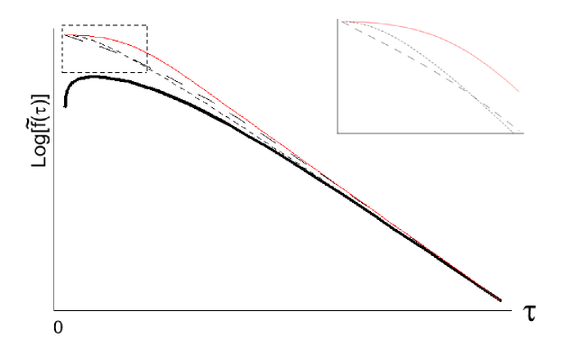
Figure 1: Plotted are the warp factors for different throat geometries as a function of $\tau$: the long dashed line is an AdS₅ geometry, the thick line is the warp factor for a KS throat with a log-correction as in [8, 3, 23, 21], the thin red line is the mass gap approximation, and the short dashed line is the exact KS warp factor. Inset:  The region near the tip, $\tau\sim 0$ is enlarged to show the differences in the warp factors. Notice that the mass gap approximation models the flattening of the KS warp factor.

While the mass gap warp factor does not satisfy the supergravity equations of motion, we will use it merely as an analytical tool to investigate the behavior of the more complicated Klebanov-Strassler throat. Since they share the same qualitative features, we will use the simpler mass gap for many of our analytic calculations; a brief analysis of the KS throat can be found in Appendix A where we show that the mass gap solution has the same qualitative behavior near the tip.

4.1 AdS₅ Throat

We will review here the results for DBI inflation in an AdS₅ throat [10, 11]. Since the mass gap warp factor (Eq.(4.12)) looks like AdS (Eq.(4.8)) for large $r$, one can consider AdS space to be the geometry of the throat far from the tip. The warp factor for the AdS space is [31]

$$f(\phi)=\frac{\lambda}{\phi^{4}}$$ (4.10)

where $\lambda=\frac{\tilde{\lambda}}{T}_{3}\sim N$, and $N$ is the $D3$ charge generating the throat.

We will consider the same form of the potential as in Eq.(3.1), and choose $H=h_{1}\phi$. Using Eq.(2.15) for the AdS warp factor for small $\phi$ we have

$$\dot{\phi}\approx-\frac{\phi^{2}}{\sqrt{\lambda}}$$ (4.11)

which gives us a late time solution of $\phi(t)\rightarrow\frac{\sqrt{\lambda}}{t}$. It should be noted that the general solution, Eq.(3.9), reduces to this solution in the limit $f_{0}=\mu^{4}/\lambda$, $f_{2}=2\mu^{2}/\lambda$ and $\mu\rightarrow 0,\ t_{f}\rightarrow\infty$. (The latter is required because the AdS solution does not reach $\phi=0$ in a finite time.) A similar calculation as done in Section 3.1 will yield the number of e-folds $N_{e}\approx h_{1}\sqrt{\lambda}$, and the level of density perturbations $\delta_{H}\approx\frac{N_{e}^{2}}{5\pi\sqrt{\lambda}}$. The rest of the observables follow a similar pattern as written above when written in terms of $N_{e}$ and we will not be concerned with their details here.

In particular, one should note that in order to get the right level of density perturbations for $N_{e}\sim 60$, $\lambda\sim 10^{14}$[13]. When viewed as a requirement on the number of $D3$ charges required to generate the throat this seems quite fine tuned ($N\sim 10^{14}$), however when viewed as a hierarchy between the radius of the $S_{3}$ at the tip of the throat and the string scale, it only requires $\lambda^{1/4}\sim R_{+}/\ell_{s}\sim 10^{3}-10^{4}$.

4.2 Mass Gap

As mentioned above, the mass gap form for the warp factor is approximately AdS₅ at large distances and constant near the tip. In terms of the inflaton field $\phi$ we have,

$$f(\phi)=\frac{\lambda}{(\phi^{2}+\mu^{2})^{2}}$$ (4.12)

where $\lambda$ is the same as in the AdS case and $\mu=\frac{R_{+}}{\ell_{s}^{2}g_{s}^{1/2}}h_{tip}$, as can be seen by requiring the warp factor Eq.(4.9) to be equal to the warping at the tip, and changing variables from $r$ to $\phi$. The mass gap in terms of the variables $f_{0}$, $f_{2}$, $f_{4}$ is given earlier in Eq.(2.4).

Now that we have a specific model for the cutoff throat we can evaluate the constraint Eq.(3.2) to evaluate whether stringy effects are important for our analysis; in particular we find $h_{tip}\geq\left(\frac{\ell_{s}}{R_{+}}\right)^{1/2}$. Requiring $h_{tip}\leq 10^{-2}$ (this is to guarantee that there is a warped region in the compactification) we have $\frac{R_{+}}{\ell_{s}}\geq 10^{4}$. Amazingly this is not too different than the tuning of $\lambda$ needed to obtain the correct value of density perturbations in the AdS model. This suggests that in order to get the right level of density perturbations for DBI inflation in the AdS region of the throat, then $\mu$ must also be large since $\mu\sim\lambda^{1/4}$. Since our constant region is large, the brane spends a significant amount of time in that region and inflation also naturally happens in the constant region of the tip.

One can also verify that even for weakly warped throats ($h_{tip}\sim 10^{-2}$) the lower bound on the inflaton mass coming from the Coulomb term Eq.(3.3) is $m_{\phi}/m_{s}\geq 10^{-14}$ and is easily satisfied. For much more strongly warped throats ($h_{tip}\ll 10^{-2}$), this requires the radius of the AdS throat to be large (requiring $N>10^{14}$ D-branes).

Plugging the mass gap solution into the Hamilton-Jacobi consistency equation Eq.(2.16), we find,

$$V_{0} = \frac{\mu^{4}}{\lambda}(1-\frac{2M_{p}^{2}h_{1}\sqrt{\lambda}}{\mu^{2}}\sqrt{1+\frac{\mu^{4}}{4h_{1}\lambda M_{p}^{4}}})$$

$$V_{2} = 3h_{1}^{2}M_{p}+\frac{2\mu^{2}}{\lambda}-\frac{2(2h_{1}^{2}M_{p}^{2}\lambda+\mu^{4})}{\lambda\mu^{2}\sqrt{1+\frac{4h_{1}^{2}M_{p}^{2}\lambda}{\mu^{4}}}}$$ (4.13)

$$V_{4} = \frac{1}{\lambda}.$$

As we will see below, inflation requires $h_{1}\sqrt{\lambda}\sim N_{e}$ to be sufficiently large, which means that Eq.(3.6) requires that the inflaton mass $m_{\phi}$ not be too small. For $\lambda\sim 10^{14}$ this requires a tuning of $\frac{m_{\phi}}{M_{p}}\geq 10^{-5}$. Notice that this is close to the typical Hubble-scale induced mass for GUT scale inflation $H\sim 10^{14}\ GeV$. Together with the requirement that $\mu<M_{p}$, which is needed in order to have a warped throat, suggests that the $V_{0}$ coming from the coupling of the scalar field to gravity must be negative. This somewhat odd result is due to the fact that for the warped throat the warp factor $f$ approaches a constant at the tip of the throat: from Eq. (2.8), our energy density $\rho$ obtains a positive constant contribution from the kinetic energy that must be canceled by a negative $V_{0}$ in order to satisfy our ansatz $H=h_{1}\phi$. Therefore our negative $V_{0}$ is an artifact of our use of the Hamilton-Jacobi formalism. As mentioned before, this does not trouble us because we have numerically simulated the equations of motion for a small, positive $V_{0}$ term and found no change to the DBI speed-limited behavior of the inflaton.

In terms of the mass-gap parameters our behavior for $\phi(t)$ is

$$\phi(t)=\mu\sqrt{1+\frac{\mu^{4}}{4h_{1}^{2}\lambda M_{p}^{4}}}\tan\left[\frac{\mu(t_{f}-t)}{\sqrt{\lambda}(1+\frac{\mu^{4}}{4h_{1}^{2}\lambda M_{p}^{4}}}\right].$$ (4.14)

As mentioned above, in the limit $\mu\rightarrow 0$, $\phi\rightarrow\mu\tan(-\mu t/\sqrt{\lambda}+\pi/2)\rightarrow\sqrt{\lambda}/t$, and we regain the late time behavior for the AdS warp factor, where the inflaton takes an infinite amount of time to reach the origin.

Since the AdS and mass gap throats have different behavior for $\phi(t)$ near the tip they also have different behaviors for the gamma factors as a function of the inflaton,

$$\gamma(\phi) \rightarrow \frac{2h_{1}\sqrt{\lambda}M_{p}^{2}}{\phi^{2}}\quad\quad\mbox{AdS Warp Throat}$$ (4.15)

$$\gamma(\phi) \rightarrow \frac{2M_{p}^{2}h_{1}\sqrt{\lambda}}{\mu^{2}+\phi^{2}}\hskip 36.135pt\mbox{Cutoff Throat}$$ (4.16)

For the AdS solution $\gamma$ becomes infinite as $\phi\rightarrow 0$, but in the mass gap solution it is finite and large. This will have implications for the non-gaussianities since $f_{NL}\propto\gamma^{2}$.

The number of e-folds for the mass gap solution is given by Eq.(3.13) with the appropriate values for $f_{0}$ and $f_{2}$: $N_{e}\approx h_{1}\sqrt{\lambda}\frac{\log(2)}{2}$. This is approximately the same expression for the number of e-folds in the AdS case, so fixing $h_{1}\sqrt{\lambda}\sim{\cal O}(100)$ will give inflation in both the AdS and constant part of the throats. Similarly, evaluating the density perturbations at $\phi\approx\mu$, we have the same expression for the density perturbations, $\delta_{H}\approx\frac{N_{e}^{2}}{\sqrt{\lambda}}$, so yet again fixing the density perturbations for the AdS part of the throat also fixes them for the constant region as well. To summarize, to fit experiment results we need a large $\lambda$, which forces $\mu$ to be large. This is significant because it means that even if inflation begins in the AdS region (as opposed to starting in the nearly constant region) then the last 60 e-folds of inflation will always be produced in the nearly constant region.

As noted for the general warp factor analysis, however, the primary conflict with observations comes from the non-gaussianities (Eq. (3.1)),

$$f_{NL}\approx 0.32\frac{M_{p}^{4}}{\mu^{4}}N_{e}^{2}.$$ (4.17)

Since we require $\mu<M_{p}$ in order to trust our supergravity analysis it appears that large non-gaussianities are predicted for inflation near the tip. For $N_{e}\sim 60$ we cannot satisfy experimental results for density perturbations and non-gaussianities simultaneously.

4.3 IR DBI Inflation

The model discussed above is known as UV DBI inflation because the inflaton moves through the throat from the UV end (large $r$) to the IR end (small $r$). This naturally happens in string constructions because, as we have seen, throats generated by fluxes have induced $D3$ charges at their tips; $\overline{D3}$ branes are then naturally attracted to the tip of the throat where they remain. $D3$ branes are then attracted to the $\overline{D3}$ at the tip of the throat, leading to the above action and inflation.

A variation on this model is to start the $D3$ brane at the tip of the throat [12]. This can arise when $p$ $\overline{D3}$ branes annihilate with the $N$ flux generated $D3$ charges and produce $N-p$ $D3$ branes at the tip. If a $\overline{D3}$ brane resides in another throat the attractive potential between the branes will pull the brane out of the throat. In particular, the potential will be of the form,

$$V=V_{0}-\frac{1}{2}m_{\phi}^{2}\phi^{2}=V_{0}-\frac{1}{2}\beta H^{2}\phi^{2};$$ (4.18)

notice that the mass term is negative, giving the direction of the force which is pulling the $D3$ out of the throat; $\beta\approx 1$ generically. The brane then moves from the IR end of the throat to the UV end of the throat. The moduli potential $V_{0}$ for the branes will be the dominant term that drives inflation. The novel part of this scenario is that the brane begins at the tip of the throat where the warp factor is approximately constant, so the geometry is important for inflation. Inflation in the IR model is obtained in a similar way as the UV model: the speed limit from the DBI action restricts how fast the inflaton can roll, so even for “relativistic” motion of the inflaton the potential stays approximately constant and inflation can proceed.

In the IR DBI model during inflation the potential dominates over the “kinetic terms” in Eq. (2.8), which gives us the following Hubble factor

$$H(\phi) = \sqrt{\frac{V_{0}-\frac{1}{2}\beta H^{2}\phi^{2}}{3M_{p}^{2}}}\approx\sqrt{\frac{V_{0}}{3M_{p}^{2}}}$$ (4.19)

$$H^{\prime}(\phi) \approx -\frac{\beta H\phi}{6M_{p}^{2}},$$ (4.20)

which combined with the Hamilton-Jacobi equations of motion give,

$$\gamma = \sqrt{1+\frac{\beta^{2}H^{2}\phi^{2}}{9(f_{0}+f_{2}\phi^{2}+f_{4}\phi^{4})}}$$ (4.21)

$$\dot{\phi} = \sqrt{\frac{f_{0}+f_{2}\phi^{2}+f_{4}\phi^{4}}{1+\frac{9(f_{0}+f_{2}\phi^{2}+f_{4}\phi^{4})}{\beta^{2}H^{2}\phi^{2}}}}$$ (4.22)

We will consider the dynamics of inflation in two distinct regions: the first region is when the warp factor is AdS-like ($f(\phi)^{-1}\approx f_{4}\phi^{4}$), and the second is when it is nearly constant ($f(\phi)^{-1}\approx f_{0}$).

Starting with AdS region of the throat, we have

$$\gamma \approx \sqrt{1+\frac{1}{9}\frac{\beta^{2}H^{2}}{f_{4}\phi^{2}}}$$ (4.23)

$$\dot{\phi} \approx \frac{\sqrt{f_{4}}\phi}{\sqrt{1+\frac{9f_{4}\phi^{2}}{\beta^{2}H^{2}}}}.$$ (4.24)

For large $\gamma$ one can solve Eq.(4.24) for the inflaton as a function of time,

$$\phi(t)\approx-\frac{\sqrt{\lambda}}{t}(1-\frac{9}{2\beta^{2}H^{2}t^{2}}),$$ (4.25)

which is the same as previously found in [12]. As previously calculated in the same paper, normalization of the density perturbations requires $\lambda\approx 10^{14}$. This has important consequences when we consider the size of $\gamma$ in this region. For the AdS region the motion of the inflaton is relativistic since $\gamma\approx\frac{\sqrt{\lambda}\beta H}{\phi}$, so for small $\phi$, $\gamma$ (and thus non-gaussianities) is large. In fact, we notice that for generic inflaton masses ($\beta\sim 1$) and the required value for $\lambda$, we must have $\phi\geq 10^{7}H/\gamma$ at 50-60 e-folds back. To be in agreement with non-gaussianity measurements ($\gamma\approx 20$) and using the upper bound $H\ll 10^{10}$ GeV found in [13] for IR DBI, trans-Planckian VEVs can be avoided, as opposed to the UV model.

In the constant region of the throat, we have

$$\gamma \approx \sqrt{1+\frac{1}{9}\frac{\beta^{2}H^{2}\phi^{2}}{f_{0}}}=\sqrt{1+\left(\frac{\phi}{\phi_{c}}\right)^{2}}$$ (4.26)

$$\dot{\phi} \approx \sqrt{f_{0}}\frac{1}{\sqrt{1+9\frac{f_{0}}{\beta^{2}H^{2}\phi^{2}}}}=\sqrt{f_{0}}\frac{1}{\sqrt{1+\left(\frac{\phi_{c}}{\phi}\right)^{2}}}$$ (4.27)

where we defined $\phi_{c}=\frac{3f_{0}^{1/2}}{\beta H}$ for simplicity. Note that $\frac{\phi_{c}}{\phi_{tip}}\approx\frac{\mu}{H\sqrt{\lambda}}$ for the mass gap solution; as noted above we expect large $\lambda$ to normalize density perturbations correctly in the AdS region, so we will assume that $\phi_{c}\ll\phi_{tip}$. The constant region of the throat can be further divided up into two regions based on our new scale $\phi_{c}$: Region 1 where $0\ll\phi\ll\phi_{c}$, and Region 2 where $\phi_{c}\ll\phi\ll\phi_{tip}$.

From Eq.(4.27) we see that in Region 1, $\gamma\approx 1$ and $\phi(t)\sim e^{\beta Ht}$ (where $\phi\rightarrow 0$ as $t\rightarrow-\infty$) so the inflaton is non-relativistic. Indeed, explicit calculation of the number of e-folds and the inflationary parameters indicates that fine tuning of the inflaton mass $\beta$ is needed to get inflation in this region,

$$\eta = -\frac{\beta}{3}$$ (4.28)

$$N_{e} = \frac{1}{\eta}\ln(\frac{\phi_{f}}{\phi_{i}}),$$ (4.29)

where $\phi_{f}$ and $\phi_{i}$ are the starting and ending points of the inflaton, respectively. The maximum value of the field in this region is at the critical value $\phi_{c}$, while the minimum value is at a warped string length $\phi_{s}$. Taking $f_{0}^{1/2}=h_{tip}^{2}m_{s}^{2}$ we have

$$N_{e}\leq\frac{1}{\eta}\ln(\frac{h_{tip}^{2}g_{s}^{1/2}}{\eta}\frac{m_{s}}{H})\approx\frac{1}{\eta}\ln(\frac{10^{-3}}{\eta}).$$ (4.30)

This is the usual slow roll $\eta$ problem (although with stronger constraints on $\beta$ due to the decreased range for $\phi$) and we will not investigate this region further.

In Region 2 near the tip of the throat ($\phi_{c}\ll\phi\ll\phi_{tip}$) the inflaton becomes relativistic since $\gamma\approx\phi/\phi_{c}$. Using Eq.(4.27) one can solve for the motion of the inflaton,

$$\phi(t)=\sqrt{f_{0}}(t+\frac{9}{2}\frac{1}{\beta^{2}H^{2}t})$$ (4.31)

which is identical to Eq.(2.37) in [13]. Here it is clear that the solution of [13] is only valid in a certain region of the constant part of the throat, and can be combined with the Region 1 solution to obtain a smooth $\phi\rightarrow 0$ limit. The number of e-folds and density perturbations in this region are

$$N_{e} = \int Hdt=\frac{H}{\dot{\phi}}\Delta\phi=\frac{H}{\mu}\sqrt{\lambda}$$ (4.32)

$$\delta_{H} = \frac{H}{M_{p}}\sqrt{\frac{\gamma}{\epsilon}}\approx\left(\frac{H}{\mu}\right)^{2}\sqrt{\lambda}=\frac{N_{e}^{2}}{\sqrt{\lambda}}$$ (4.33)

where in the last step we inserted the mass-gap parameters. It is possible that in the IR model some e-folds occur in this region, with the rest of the e-folds occurring in the AdS part of the throat. One will also generically have problems associated with large non-gaussianities due to the large value of $\gamma$, which near $\phi_{tip}$ for the mass gap parameters goes like $\gamma\approx\frac{H\sqrt{\lambda}}{\mu}$. As in the AdS case, however, staying below the upper bound on $H$ allows non-gaussianities within observational limits.

5 Discussion

In this paper we have considered the effects of a cutoff throat on DBI inflation. We focused on constructions where the brane spends a significant amount of time in a region of nearly constant warping near the tip of the throat. To study these types of throats we assumed that the nearly constant region was larger than a string length from the tip (Eq.(3.2)). This may or may not be more stringent than the requirement that we obtain enough e-folds (Eq.(3.14)) and the right level of density perturbations (Eq.(3.31)), since the results depend on the specific geometry of the warped throat. For a weakly warped ($h_{tip}\sim 10^{-2}$) Klebanov-Strassler throat, we showed that such assumptions are satisfied .

In both the UV and IR models of DBI inflation the geometry near the tip can be important. In the former, since the tip is the last region the D-brane experiences before stringy effects (such as annihilation) become important, significant inflation in this region can affect inflationary observables. In particular, we find that for generically warped throats 60 e-folds of inflation can happen near the tip, however the production of large non-gaussian fluctuations seems to be a generic prediction. From Eq.(3.33) we see that for a small enough hierarchy between the Planck and string scale, and a large enough hierarchy between the inflaton mass and the Planck scale the non-gaussianities can be sufficiently small. It is not clear, however, if this amounts to a fine tuning of the parameters of the model.

We find that the requirement for enough inflation in the constant region of the Klebanov-Strassler throat, modeled by the mass gap approximation, ($R_{+}/\ell_{s}\geq 10^{4}$) is similar to the requirement that the level of density perturbations for inflation in the AdS throat yield the correct value ($R_{+}/\ell_{s}\sim 10^{3}-10^{4}$). This implies that it is important to consider inflation at the tip for UV DBI inflation models. However, for the mass gap model of the Klebanov-Strassler throat we find large non-gaussianities, above the observational limits, for all values of the mass gap parameter $\mu$ consistent with our supergravity analysis. As discussed above, this may be avoided by considering other types of throats and compactifications.

In the IR model of DBI inflation, the geometry near the tip affects the early time behavior of the inflaton. In particular, we find that very near the tip the inflaton is not speed limited (i.e. $\gamma\approx 1$) and so, without fine tuning of the inflaton mass, we do not expect inflation there. Further from the tip, but still in the nearly constant region of the throat, the inflaton becomes relativistic and the level of non-gaussianities quickly grow larger. Normalization of density perturbations in both the tip and AdS regions of the throat requires tuning of the AdS curvature scale as in the UV model, however agreement with non-gaussianity observations constrains the Hubble scale of inflation to be smaller than $10^{13}$ GeV (as is typical for GUT scale inflation).

Throughout this work we have considered only contributions to the inflaton from the transverse radial mode between the D-branes - it would be interesting to extend this work to consider the effects of the angular coordinates on DBI inflation similar to the scenario of [6]. Furthermore, since the inflationary behavior does not seem to depend on whether we have a D-brane or $\overline{D}$-brane falling into the throat, one could imagine an $\overline{D}$-brane attracted to the tip of the throat by the $D3$ charge of the fluxes, where it collides with a stack of other $\overline{D3}$ already at the tip. Reheating then occurs in the collision process between the $\overline{D3}$s. Since we have seen that the D-brane in the UV model is highly relativistic at the tip of the throat, the annihilation [32] and collision process may be significantly altered along the lines of [33], and may have interesting observational consequences. In addition, the formation of cosmic strings from the annihilation of highly relativistic branes is a relatively unexplored subject, and may yield different post-annihilation production and properties than the non-relativistic case [9, 34]. We hope to return to these issues in the future.

Appendix A The KS Throat

The purpose of this section is to show that the mass-gap solution accurately models the dynamics near the tip, and is a good qualitative approximation to the full KS throat. For the warped throat we take the form of the metric used in [22, 23],

$$ds_{10}^{2}=\tilde{f}^{-1/2}(\tau)\eta_{\mu\nu}dx^{\mu}dx^{\nu}+\tilde{f}^{1/2}(\tau)ds_{6}^{2}$$ (A.1)

where $\tau$ is the separation between the D-branes in the throat and the warp factor $\tilde{f}(\tau)$ is defined by

$$\tilde{f}(\tau) = 2^{2/3}(g_{s}M\alpha^{\prime})^{2}\epsilon^{-8/3}I(\tau)$$ (A.2)

$$I(\tau) = \int_{\tau}^{\infty}\frac{x\coth(x)-1}{\sinh^{2}(x)}(\sinh(2x)-2x)^{1/3}dx.$$ (A.3)

$\epsilon$ is a small real number that is related the deformation of the warped conifold. If we take $\tau\rightarrow\infty$ then we recover the AdS approximation, where $\tau$ is redefined in terms of a radial coordinate $r$. We are interested in keeping the $\tau$ coordinate and observing its behavior near the tip, so the form of the metric we will use is

$$ds_{10}^{2}=\tilde{f}^{-1/2}(\tau)\eta_{\mu\nu}dx^{\mu}dx^{\nu}+\tilde{f}^{1/2}(\tau)\left(\frac{\epsilon^{4/3}}{6K^{2}(\tau)}d\tau^{2}+\dots\right)$$ (A.4)

where

$$K(\tau)=\frac{(\sinh(2\tau)-2\tau)^{1/3}}{2^{1/3}\sinh(\tau)}.$$ (A.5)

The next step is to calculate the DBI action for the KS throat. To do this efficiently we will use the definitions:

$$h(\tau) = \frac{2^{2/3}(g_{s}M\alpha^{\prime})^{2}I(\tau)\epsilon^{-4/3}}{K^{2}(\tau)}$$ (A.6)

$$\gamma = \frac{1}{\sqrt{1-f(\tau)\dot{\tau}^{2}}}$$ (A.7)

The action is then

$$S_{KS}=-T_{D3}\int d^{4}x\sqrt{g}~{}\left(\tilde{f}^{-1}(\tau)\left(\sqrt{1-h(\tau)\dot{\tau}^{2}}-1\right)-V(\tau)\right)$$ (A.8)

To consider inflation from the radial coordinate $\tau$ we will define a canonically normalized scalar field $\varphi$ by expanding the DBI action for small $\dot{\tau}$,

$$S_{KS} \approx \int d^{4}x\sqrt{g}\left(\frac{1}{2}T_{D3}\frac{h(\tau)}{\tilde{f}(\tau)}\dot{\tau}^{2}+T_{D3}V(\tau)\right)$$ (A.9)

$$= \int d^{4}x\sqrt{g}\left(\frac{1}{2}\dot{\varphi}^{2}+V(\varphi)\right)$$ (A.10)

where $\tau\approx\frac{K(\tau\rightarrow 0)}{T_{D3}^{1/2}\epsilon^{2/3}}~{}\varphi=\left(\frac{2}{3}\right)^{1/3}\frac{1}{T_{D3}^{1/2}\epsilon^{2/3}}~{}\varphi$ for small $\tau$. Rewriting Eq.(A.8) in terms of the new scalar field $\varphi$:

$$S_{KS}=-\int d^{4}x\sqrt{g}\left(f(\varphi)^{-1}(\sqrt{1-f(\varphi)\dot{\varphi}^{2}}-1)-V(\varphi)\right).$$ (A.11)

This has the same form as the DBI action considered in Eq.(2.2) for the rescaled warp factor $f(\varphi)=\tilde{f}(\varphi(\tau))/T_{D3}$. In the small $\tau$ expansion we find $\tilde{f}(\tau)^{-1}\approx 2^{-2/3}(g_{s}M\alpha^{\prime})^{-2}\epsilon^{8/3}(b_{0}+b_{2}\tau^{2}+b_{4}\tau^{4})$, where $b_{0}$, $b_{2}$, and $b_{4}$ are constants of ${\cal{O}}(1)$. This warp factor is well approximated by the mass gap solution after changing to the canonically normalized field $\varphi$.

Appendix B Non-Gaussianities

In this section we discuss non-gaussianities in DBI inflation for a generic form of the warp factor. The results of non-gaussianity for general single field inflation can be found in [35]. Here we assume the non-gaussianity is large due to large $\gamma$, and so we can adopt the method of [11].

Using our DBI action (Eq.(2.2)), our general warp factor (Eq.(2.3)), a FRW metric for the non-compact space, and a generic form of the potential $V=V_{0}+V_{2}\phi^{2}+V_{4}\phi^{4}$, we introduce perturbations to our scalar field

$$\phi\rightarrow\phi(t)+\alpha(x,t).$$ (B.1)

Non-gaussianities come from the third order interactions in our Lagrangian due to the perturbation $\alpha(x,t)$,

$${\cal{L}}_{3} = -a(t)^{3}\left[\frac{\gamma^{5}\dot{\phi}}{2(f_{0}+f_{2}\phi^{2}+f_{4}\phi^{4})}\dot{\alpha}^{3}-\frac{\gamma^{3}\dot{\phi}}{2a^{2}(f_{0}+f_{2}\phi^{2}+f_{4}\phi^{4})}\dot{\alpha}(\nabla\alpha)^{2}\right.$$

$$\left.+\frac{\gamma^{3}\phi(f_{2}+2f_{4}\phi^{2})\dot{\phi}^{2}}{2a^{2}(f_{0}+f_{2}\phi^{2}+f_{4}\phi^{4})^{2}}\alpha(\nabla\alpha)^{2}\right.$$

$$\left.+\frac{\gamma^{3}\dot{\phi}^{3}}{2(f_{0}+f_{2}\phi^{2}+f_{4}\phi^{4})^{4}}\left(-f_{0}^{2}f_{2}+19f_{2}f_{4}^{2}\phi^{8}+10f_{4}^{3}\phi^{10}\right.\right.$$

$$\left.\left.+\phi^{2}(2f_{0}(f_{2}^{2}-3f_{0}f_{4})+3f_{2}^{2}\gamma^{2}\dot{\phi}^{2})+4f_{4}\phi^{6}(3f_{2}^{2}+f_{0}f_{4}+3f_{4}\gamma^{2}\dot{\phi}^{2})\right.\right.$$

$$\left.\left.+f_{2}\phi^{4}(3f_{2}^{2}+2f_{0}f_{4}+12f_{4}\gamma^{2}\dot{\phi}^{2})\right)\dot{\alpha}\alpha^{2}-\frac{3\gamma^{5}\phi(f_{2}+2f_{4}\phi^{2})\dot{\phi}^{2}}{2(f_{0}+f_{2}\phi^{2}+f_{4}\phi^{4})^{2}}\dot{\alpha}^{2}\alpha\right.$$

$$\left.+\frac{\phi}{2\gamma}\left(8(f_{4}(-1+\gamma)-V_{4}\gamma)-\frac{4f_{4}\gamma^{2}\dot{\phi}^{2}}{f_{0}+f_{2}\phi^{2}+f_{4}\phi^{4}}\right.\right.$$

$$\left.\left.+\frac{\gamma^{4}\dot{\phi}^{4}}{(f_{0}+f_{2}\phi^{2}+f_{4}\phi^{4})^{4}}(f_{2}+2f_{4}\phi^{2})(f_{0}f_{2}-\phi^{2}(f_{2}^{2}-6f_{0}f_{4}+f_{4}\phi^{2}(f_{2}+2f_{4}\phi^{2})))\right.\right.$$

$$\left.\left.-\frac{\gamma^{6}\phi^{2}\dot{\phi}^{6}(f_{2}+2f_{4}\phi^{2})^{3}}{(f_{0}+f_{2}\phi^{2}+f_{4}\phi^{4})^{5}}\right)\alpha^{3}\right]$$

The behavior of the non-gaussian fluctuations will be dominated by the small $\phi$ (alternatively, late time) behavior of the perturbations near the tip of the throat. Plugging our value for $\dot{\phi}$ from Eq.(2.15), we can evaluate the leading $\phi$ behavior of ${\cal{L}}_{3}$. Of the terms in Eq.(B), the $\dot{\alpha}^{3}$ and $\dot{\alpha}\nabla{\alpha}^{2}$ are dominant for small $\phi$, and produce the same results as in [11, 13]. The results for these terms hold for all choices of warp factor.

Naively the first term from the $\dot{\alpha}\alpha^{2}$ contribution ($\propto-f_{0}^{2}f_{2}$) can also possibly contribute to the non-gaussianities. Using the procedure outlined in [11] and evaluating this term for the mass gap solution, we find that it produces non-gaussianities of ${\cal{O}}(\gamma)$, which is subleading in the limit of large $\gamma$. Since the procedure in [11] only produces the leading non-gaussianities, ${\cal{O}}(\gamma)$ contributions will be dropped.

References

- [1] G. Dvali, S.H.H. Tye, Phys. Lett. B. 450, 72 (1999), [arXiv:hep-th/9812483].
- [2] C.P. Burgess, M. Majumdar, D. Nolte, F. Quevedo, G. Rajesh, R.J. Zhang, JHEP 0107, 047 (2001), [arXiv:hep-th/0105204]; G. R. Dvali, Q. Shafi and S. Solganik, [arXiv:hep-th/0105203]; G. Shiu and S. H. H. Tye, Phys. Lett. B 516, 421 (2001) [arXiv:hep-th/0106274]; C.P. Burgess, P. Martineau, F. Quevedo, G. Rajesh and R. J. Zhang, JHEP 0203, 052 (2002) [arXiv:hep-th/0111025]; H. Firouzjahi and S. H. H. Tye, Phys. Lett. B 584, 147 (2004) [arXiv:hep-th/0312020]; C. P. Burgess, J. M. Cline, H. Stoica and F. Quevedo, JHEP 0409, 033 (2004) [arXiv:hep-th/0403119]; N. Iizuka, S.P. Trivedi, Phys.Rev. D70 (2004) 043519 [arXiv:hep-th/0403203]; A. Buchel, A. Ghodsi, Phys.Rev. D70 (2004) 126008 [arXiv:hep-th/0404151]; A. Buchel, [arXiv:hep-th/0601013].
- [3] S. Kachru, R. Kallosh, A. Linde, J. Maldacena, L. McAllister, S. Trivedi, JCAP 0310 (2003) 013 [arXiv:hep-th/0308055].
- [4] J. Garcia-Bellido, R. Rabadan, R. Zamora, JHEP 0201, 036 (2002), [arXiv:hep-th/0112147]; R. Blumenhagen, B. Kors, D. Lust and T. Ott, Nucl. Phys. B 641, 235 (2002) [arXiv:hep-th/0202124]; N. Jones, H. Stoica, S.H.H. Tye, JHEP 0207, 051 (2002), [arXiv:hep-th/0203163]; M. Gomez-Reino and I. Zavala, JHEP 0209, 020 (2002) [arXiv:hep-th/0207278]. S. Shandera, B. Shaler, H. Stoica, S.H.H. Tye, JCAP 0402, 013 (2004), [arXiv:hep-th/0311207].
- [5] F. Quevedo, Class. Quant. Grav 19, 5721-5779C (2002) [arXiv:hep-th/0210292]; K. Dasgupta, C. Herdeiro, S. Hirano and R. Kallosh, Phys. Rev. D 65, 126002 (2002) [arXiv:hep-th/0203019]; G. Shiu and I. Wasserman, Phys. Lett. B 541, 6 (2002) [arXiv:hep-th/0205003]; G. Shiu, S. H. H. Tye and I. Wasserman, Phys. Rev. D 67, 083517 (2003) [arXiv:hep-th/0207119]; J. J. Blanco-Pillado et al., JHEP 0411, 063 (2004) [arXiv:hep-th/0406230]; J. J. Blanco-Pillado et al., [arXiv:hep-th/0603129]; H. Firouzjahi and S. H. H. Tye, JCAP 0503, 009 (2005) [arXiv:hep-th/0501099]; K. Becker, M. Becker and A. Krause, Nucl. Phys. B 715, 349 (2005) [arXiv:hep-th/0501130]; A. Westphal, JCAP 0511 (2005) 003 [arXiv:hep-th/0507079]; E. Papantonopoulos, I. Pappa, V. Zamarias, [arXiv:hep-th/0601152].
- [6] O. DeWolfe, S. Kachru and H. L. Verlinde, JHEP 0405, 017 (2004) [arXiv:hep-th/0403123].
- [7] G. Shiu, S. H. H. Tye and I. Wasserman, Phys. Rev. D 67, 083517 (2003) [arXiv:hep-th/0207119]; N. Barnaby, C. P. Burgess and J. M. Cline, JCAP 0504, 007 (2005), [arXiv:hep-th/0412040]; D. Chialva, G. Shiu and B. Underwood, JHEP 0601, 014 (2006) [arXiv:hep-th/0508229]; A. R. Frey, A. Mazumdar and R. Myers, Phys. Rev. D73, 026003 (2006), [arXiv:hep-th/0508139]; X. Chen and S. H. H. Tye, [arXiv:hep-th/0602136]; P. Langfelder, [arXiv:hep-th/0602296].
- [8] L. Kofman and P. Yi, Phys. Rev. D 72, 106001 (2005) [arXiv:hep-th/0507257].
- [9] S. Sarangi and S. H. H. Tye, Phys. Lett. B 536, 185 (2002) [arXiv:hep-th/0204074]; G. Shiu, [arXiv:hep-th/0210313]; N. T. Jones, H. Stoica and S. H. H. Tye, Phys. Lett. B 563, 6 (2003) [arXiv:hep-th/0303269]; L. Pogosian, S. H. H. Tye, I. Wasserman and M. Wyman, Phys. Rev. D 68, 023506 (2003) [arXiv:hep-th/0304188]; T. Damour and A. Vilenkin, Phys. Rev. D 71, 063510 (2005) [arXiv:hep-th/0410222]; N. Barnaby, A. Berndsen, J. M. Cline and H. Stoica, JHEP 0506, 075 (2005) [arXiv:hep-th/0412095]; G. Dvali, R. Kallosh and A. Van Proeyen, JHEP 0401 (2004) 035 [hep-th/0312005]; G. Dvali and A. Vilenkin, JCAP 0403 (2004) 010 [hep-th/0312007]; K. Dasgupta, J. P. Hsu, R. Kallosh, A. Linde and M. Zagermann, [hep-th/0405247]; B. Chen, M. Li, J. She, JHEP 0506 (2005) 009, [arXiv:hep-th/0504040]; E. J. Copeland, R. C. Myers and J. Polchinski, JHEP 0406, 013 (2004) [arXiv:hep-th/0312067].
- [10] E. Silverstein and D. Tong, Phys. Rev. D 70, 103505 (2004) [arXiv:hep-th/0310221].
- [11] M. Alishahiha, E. Silverstein and D. Tong, Phys. Rev. D 70, 123505 (2004) [arXiv:hep-th/0404084].
- [12] X. Chen, Phys.Rev. D71 (2005) 063506 [arXiv:hep-th/0408084]; JHEP 0508 (2005) 045 [arXiv:hep-th/0501184].
- [13] X. G. Chen, [arXiv:astro-ph/0507053].
- [14] H. Verlinde, Nucl. Phys. B580 (2000) 264, [arXiv:hep-th/9906182].
- [15] S. Gukov, C. Vafa and E. Witten, “CFT’s from Calabi-Yau four-folds,” Nucl. Phys. B 584, 69 (2000) [Erratum-ibid. B 608, 477 (2001)] [arXiv:hep-th/9906070].
- [16] K. Dasgupta, G. Rajesh and S. Sethi, “M theory, orientifolds and G-flux,” JHEP 9908, 023 (1999) [arXiv:hep-th/9908088].
- [17] B. R. Greene, K. Schalm and G. Shiu, “Warped compactifications in M and F theory,” Nucl. Phys. B 584, 480 (2000) [arXiv:hep-th/0004103].
- [18] S. B. Giddings, S. Kachru and J. Polchinski, Phys. Rev. D 66, 106006 (2002) [arXiv:hep-th/0105097].
- [19] S. Kachru, R. Kallosh, A. Linde, S.P. Trivedi, Phys. Rev. D, 68, 046005 (2003), [arXiv:hep-th/0301240].
- [20] I. R. Klebanov and M. J. Strassler, JHEP 0008, 052 (2000) [arXiv:hep-th/0007191].
- [21] I. R. Klebanov and A. A. Tseytlin, Nucl. Phys. B 578, 123 (2000) [arXiv:hep-th/0002159].
- [22] P. Candelas and X. C. de la Ossa, Nucl. Phys. B 342, 246 (1990); R. Minasian and D. Tsimpis, Nucl. Phys. B 572, 499 (2000), [arXiv:hep-th/9911042]; K. Ohta and T. Yokono, JHEP 0002, 023 (2000), [arXiv:hep-th/9912266]; H. Firouzjahi and S. H. H. Tye, JHEP 0601, 136 (2006) [arXiv:hep-th/0512076].
- [23] C. P. Herzog, I. R. Klebanov and P. Ouyang, [arXiv:hep-th/0108101];
- [24] S. E. Shandera and S. H. H. Tye, [arXiv:hep-th/0601099].
- [25] D.N. Spergel et. al, [arXiv:astro-ph/0603449].
- [26] A. G. Muslimov, Class. Quant. Grav. 7, 231 (1990); D. S. Salopek and J. R. Bond, Phys. Rev. D 42, 3936 (1990); J. E. Lidsey, Phys. Lett. B 273, 42 (1991).
- [27] R. D’Auria, S. Ferrara and M. Trigiante, [arXiv:hep-th/0407138]; L. Andrianopoli, R. D’Auria, S. Ferrara and M. A. Lledo, JHEP 0303, 044 (2003) [arXiv:hep-th/0302174]; P. K. Tripathy and S. P. Trivedi, JHEP 0303, 028 (2003) [arXiv:hep-th/0301139]; C. Angelantonj, R. D’Auria, S. Ferrara and M. Trigiante, Phys. Lett. B 583, 331 (2004) [arXiv:hep-th/0312019]; A. R. Frey and J. Polchinski, Phys. Rev. D 65, 126009 (2002) [arXiv:hep-th/0201029]; S. Kachru, M. B. Schulz and S. Trivedi, JHEP 0310, 007 (2003) [arXiv:hep-th/0201028]. S. E. Shandera, JCAP 0504, 011 (2005) [arXiv:hep-th/0412077].
- [28] O. DeWolfe and S.B. Giddings, Phys. Rev. D67 (2003) 066008, [arXiv:hep-th/0208123]; S.B. Giddings and A. Maharana, [arXiv:hep-th/0507158]; A. Frey and A. Maharana, [arXiv:hep-th/0603233].
- [29] H. Kodama and K. Uzawa, JHEP 0507, 061 (2005) [arXiv:hep-th/0504193].
- [30] S. Kachru, J. Pearson and H. L. Verlinde, JHEP 0206, 021 (2002) [arXiv:hep-th/0112197].
- [31] L. Randall and R. Sundrum, Phys. Rev. Lett. 83, 3370 (1999) [arXiv:hep-ph/9905221].
- [32] P. Yi, Nucl. Phys. B 550, 214 (1999) [arXiv:hep-th/9901159]; O. Bergman, K. Hori and P. Yi, Nucl. Phys. B 580, 289 (2000) [arXiv:hep-th/0002223]; G. W. Gibbons, K. Hori and P. Yi, Nucl. Phys. B 596, 136 (2001) [arXiv:hep-th/0009061]; A. Sen, J. Math. Phys. 42, 2844 (2001) [arXiv:hep-th/0010240]; G. Gibbons, K. Hashimoto and P. Yi, JHEP 0209, 061 (2002) [arXiv:hep-th/0209034]; B. Chen, M. Li and F. L. Lin, JHEP 0211, 050 (2002) [arXiv:hep-th/0209222]; P. Mukhopadhyay and A. Sen, JHEP 0211, 047 (2002) [arXiv:hep-th/0208142]; S. J. Rey and S. Sugimoto, Phys. Rev. D 67, 086008 (2003) [arXiv:hep-th/0301049]; A. Sen, JHEP 0204, 048 (2002) [arXiv:hep-th/0203211]; JHEP 0207, 065 (2002) [arXiv:hep-th/0203265]; Mod. Phys. Lett. A 17, 1797 (2002) [arXiv:hep-th/0204143]; Phys. Rev. Lett. 91, 181601 (2003) [arXiv:hep-th/0306137]; [arXiv:hep-th/0410103]; N. Lambert, J. Liu, J. Maldacena, [arXiv:hep-th/0303139]; M. Gutperle and P. Yi, JHEP 0501, 015 (2005) [arXiv:hep-th/0409050]; J. Shelton, JHEP 0501 (2005) 037 [arXiv:hep-th/0411040]; N.T. Jones, L. Leblond, S.H.H. Tye, JHEP 0310 (2003) 002, [arXiv:hep-th/0307086]. X. Chen, Phys.Rev. D70 (2004) 086001 [arXiv:hep-th/0311179].
- [33] L. McAllister and I. Mitra, JHEP 0502, 019 (2005) [arXiv:hep-th/0408085].
- [34] For some recent reviews, see, e.g., J. Polchinski, [arXiv:hep-th/0412244]; T. W. B. Kibble, [arXiv:astro-ph/0410073]; A. Vilenkin, [arXiv:hep-th/0508135].
- [35] X. Chen, M. x. Huang, S. Kachru and G. Shiu, arXiv:hep-th/0605045.