Time-Dependent Supersymmetric Solutions in M-Theory
and the Compactification-Decompactification Transition

Abstract

We show that the diagonal light-like solution with 16 supersymmetries in eleven-dimensional supergravity derived in our previous paper can be generalised to non-diagonal solutions preserving the same number of supersymmetries. Although the metric coefficients of this generalised light-like solution depend on only a single null coordinate, this class of solutions contains a subclass equivalent to the class of solutions found by Bin Chen that are dependent on the spatial coordinates. Utilising these solutions, we construct toroidally compactified solutions that smoothly connect a static compactified region with a dynamically decompactifying region along a null hypersurface.

1 Introduction

In cosmology based on higher-dimensional unified theories, the dynamics of moduli associated with compactification are of crucial importance in constructing a realistic universe model as well as in investigating the early evolution of the universe.

This problem is closely related to the stability of vacua. In general, it is often implicitly assumed that a supersymmetric vacuum is stable. This is generally correct for a supersymmetric theory without gravity. However, in supergravity, a supersymmetric vacuum can become unstable with respect to small perturbations if it belongs to a continuous set of degenerate vacua, that is, if there exist (massless) moduli degrees of freedom. In general, such instabilities are associated with dynamically increasing supersymmetry breaking, as in the case of the size-modulus instability for vacua with flux in warped compactifications of type IIB supergravity[1, 2, 3]. Instabilities of this type affect the expansion law of the universe significantly and often produce naked singularities or a big-rip singularity[1, 2]. There can be other types of instabilities that connect two different supersymmetric vacua and are associated with topological change of the internal space[4, 5], such as the flop transition[6, 7] and the conifold transition[8, 9, 10]. These types of transitions are also associated with supersymmetry breaking or singularities.

In the treatment of a singularity appearing in our spacetime, the usual approach based on general relativity offers little insight. It is here that superstring theories and M-theory are expected to be useful. In fact, recent studies of time-dependent supersymmetric solutions in string theories and M-theory have cast new light on this problem.[11, 12, 13, 14, 15, 16, 17, 18, 19, 20, 21, 22, 23, 24, 25] In particular, various time-dependent solutions with partial supersymmetry have been found and used to study the nature of singularities in the context of cosmology. Solutions with partial supersymmetry are important because they allow us to investigate nonperturbative regions of our spacetime. In this case, it has been argued that such a singularity can be described perturbatively in terms of dual matrix theories. It would be interesting to explore this possibility further and obtain more insight into singularities, instabilities and other aspects of such time-dependent solutions.

The main purpose of the present paper is to point out that there exists another type of instability in M-theory, that is, a dynamical instability of extra dimensions described by an exactly supersymmetric solution. Because supersymmetric solutions in supergravity always have time-like or null Killing vectors[26, 27, 28, 29, 30, 31, 32, 33], dynamical phenomena can be described by supersymmetric solutions only when they have null Killing vectors. Recently, we found a class of such solutions with 16 supersymmetries in M-theory with a non-trivial 4-form flux[16]. These light-like solutions are represented by a diagonal metric whose components depend on only a single null coordinate, $u$. In the present paper, we slightly generalise these solutions to a class with a non-diagonal metric preserving the spatial-coordinate independence and study their toroidal compactification. In particular, we explicitly construct the compactification of supersymmetric regular light-like solutions for which the internal space is static in the region of the spacetime satisfying $u<0$ and dynamically expands as $u\rightarrow\infty$. We also point out that solutions of this type can be used to construct a supersymmetric solution that describes the creation and expansion of a stable compactified region in an asymptotically decompactifying background.

In this construction of dynamical compactification, it is not essential that the metric be non-diagonal. However, with this generalisation to non-diagonal solutions, we can investigate the problem in a quite wide class of solutions with 16 supersymmetries, in spite of the fact that the metric is independent of the spatial coordinates. In fact, we show that through appropriate coordinate transformations, the apparently more general solutions with spatial-coordinate dependence found by Bin Chen[15] can be mapped to a subclass of our generalised light-like solutions.

The present paper is organised as follows. In the next section, we show that the diagonal solutions we derived previously can be generalised to non-diagonal solutions preserving 16 supersymmetries. Then, we prove that Bin Chen’s solutions can be transformed into a subclass of our generalised light-like solutions. Furthermore, we illustrate this point explicitly for the Kowalski-Glikman solution[34] with 32 supersymmetries. In §3, we study basic geometrical properties of our solutions. In particular, we determine the common maximal isometry group of our class of solutions. We also comment on some exceptional solutions with higher symmetries. With these preparations, we investigate toroidal compactification of our solutions and construct dynamically decompactifying solutions in §4. Section 5 is devoted to a summary and discussion.

2 Light-like solutions in M-theory

2.1 Generalised light-like solutions

The bosonic sector of the $D=11$ minimal supergravity consists of a spacetime metric $g_{MN}$ and a 4-form flux $F_{4}$. Their field equations are given by

$$R_{MN}=\frac{1}{12}F_{MP_{1}P_{2}P_{3}}F_{N}{}^{P_{1}P_{2}P_{3}}-\frac{1}{6}F_{4}\cdot F_{4}g_{MN},$$ (1a)

$$dF_{4}=0,\quad d{}*\!F_{4}+\frac{1}{4}F_{4}\wedge F_{4}=0.$$ (1b)

Here and in the following, we define the inner product of two $p$-forms as

$$\alpha_{p}\cdot\beta_{p}=\frac{1}{p!}\alpha_{M_{1}\cdots M_{p}}\beta^{M_{1}\cdots M_{p}}.$$ (2)

Let us consider the spacetime whose metric is given by

$$ds^{2}=-2dudv+g_{ij}(u)dx^{i}dx^{j}.$$ (3)

Here, $g_{ij}(u)$ is a general non-degenerate matrix depending on only the coordinate $u$. With respect to the null frame,

$$\theta^{-}=-du,\quad\theta^{+}=dv,\quad\theta^{I}=\theta^{I}_{i}(u)dx^{i},$$ (4a)

$$e_{-}=-\partial_{u},\quad e_{+}=\partial_{v},\quad e_{I}=e_{I}^{i}(u)\partial_{i},$$ (4b)

where $\theta^{I}_{i}e_{J}^{i}=\delta^{I}_{J}$, the non-vanishing components of the Riemann curvature tensor are given by

$$R_{-i-j}=\left(-\frac{1}{2}\ddot{g}+\frac{1}{4}\dot{g}g^{-1}\dot{g}\right)_{ij}.$$ (5)

Throughout this paper, a dot represents differentiation with respect to $u$.

From the above, it follows that the components of the Ricci tensor other than $R_{--}$ vanish. Hence, from the Einstein equations, we obtain

$$0\equiv R_{++}=\frac{1}{12}F_{+ijk}F_{+}{}^{ijk},$$ (6a)

$$0\equiv R_{+-}=\frac{1}{6}\left(F_{+-ij}F_{+-}{}^{ij}+\frac{1}{4!}F_{ijkl}F^{ijkl}\right).$$ (6b)

These equations are equivalent to

$$F_{+-ij}=F_{+ijk}=F_{ijkl}=0.$$ (7)

Under these conditions, $F_{4}\cdot F_{4}$ vanishes, and we can easily see that the Einstein equations reduce to the single equation

$$R_{--}\equiv{\rm Tr}\left(-\frac{1}{2}g^{-1}\ddot{g}+\frac{1}{4}g^{-1}\dot{g}g^{-1}\dot{g}\right)=\frac{1}{12}F_{-ijk}F_{-}{}^{ijk}.$$ (8)

Now, the 4-form flux can be written

$$F_{4}=\frac{1}{3!}F_{-ijk}\theta^{-}\wedge dx^{i}\wedge dx^{j}\wedge dx^{k}=-du\wedge F_{-},$$ (9)

where

$$F_{-}=\frac{1}{3!}F_{-ijk}dx^{i}\wedge dx^{j}\wedge dx^{k}.$$ (10)

Hence, the field equation $dF_{4}=0$ yields

$$\partial_{v}F_{-}=0,\quad d_{x}F_{-}=0.$$ (11)

Because $F_{4}\wedge F_{4}=0$ in the present case, the remaining field equation for $F_{4}$ becomes $d{}*\!F_{4}=0$. For a $p$-form $\omega_{p}$ on $X_{9}\ni(x^{i})$, we have

$${}*\!(du\wedge\omega_{p})=(-1)^{10-p}du\wedge{}*\!_{X}\omega_{p},$$ (12)

where ${}*\!_{X}$ denotes the Hodge dual on $X_{9}$ with respect to the metric $g_{ij}dx^{i}dx^{j}$. Hence, the equation $d{}*\!F_{4}=0$ is equivalent to

$$d_{x}{}*\!_{X}F_{-}=0.$$ (13)

Thus, $F_{-}$ should be a $v$-independent harmonic 3-form on the space $X_{9}$. In particular, if we require that the curvature of the spacetime be bounded everywhere, (8) is consistent only when $F_{-ijk}$ is independent of $v$ and $x^{i}$. Hereafter, let us assume this. The general regular solution to (1a) and (1b) with the metric form (3) is then given by a set of functions of $u$, which we denote $g_{ij}(u)$ and $F_{-ijk}(u)$, satisfying (8). This solution reduces to the solution found in Ref. Ishino.T&KodamaOhta2005 when $g_{ij}(u)$ is diagonal.

2.2 Supersymmetry

In the Killing spinor equation

$$(\nabla_{M}+T_{M})\epsilon=0,$$ (14)

with

$$\nabla_{M}=\partial_{M}+\frac{1}{4}\omega_{abM}\Gamma^{ab},$$ (15)

and

$$T_{M}=\frac{1}{288}\left(\Gamma_{M}{}^{P_{1}\cdots P_{4}}-8\delta^{P_{1}}_{M}\Gamma^{\cdots P_{4}}\right)F_{P_{1}\cdots P_{4}},$$ (16)

the connection coefficients for the metric (3) with respect to the null frame (4) are given by

$$\omega_{++}=\omega_{+-}=\omega_{--}=\omega_{+I}=0,$$ (17a)

$$\omega_{-I}=h_{IJ}\theta^{J},\quad\omega_{IJ}=\Omega_{IJ}\theta^{-},$$ (17b)

with

$$h_{IJ}=\frac{1}{2}e_{I}^{i}e_{J}^{j}\dot{g}_{ij},\quad\Omega_{IJ}=e^{i}_{[J}\dot{\theta}_{I]i},$$ (18)

and the matrices $T_{M}$ are expressed as

$$T_{-} = \frac{1}{72}(\Gamma^{+}\Gamma^{-}-3)\Gamma^{IJK}F_{-IJK},$$ (19a)

$$T_{+} = 0,$$ (19b)

$$T_{I} = \frac{1}{72}\left(-\Gamma_{I}{}^{JKL}F_{-JKL}+6\Gamma^{JK}F_{-IJK}\right)\Gamma^{-},$$ (19c)

where $\Gamma^{\pm}=(\Gamma^{10}\pm\Gamma^{0})/\sqrt{2}$. Therefore, the Killing spinor equation can be written

$$\left[\partial_{-}+\frac{1}{4}\Omega_{IJ}\Gamma^{IJ}+\frac{1}{72}(\Gamma^{+}\Gamma^{-}-3)\Gamma^{IJK}F_{-IJK}\right]\epsilon=0,$$ (20a)

$$\partial_{+}\epsilon=0,$$ (20b)

$$\partial_{I}\epsilon+\left[-\frac{1}{2}h_{IJ}\Gamma^{J}+\frac{1}{72}\left(-F_{-JKL}\Gamma_{I}{}^{JKL}+6F_{-IJK}\Gamma^{JK}\right)\right]\Gamma^{-}\epsilon=0.$$ (20c)

Here, note that the quantities $\Gamma^{I\cdots J}$ are constant matrices and that $h_{IJ},\Omega_{IJ}$ and $F_{-IJK}$ are functions of only $u$.

Now, let $\zeta$ be a constant spinor satisfying

$$\Gamma^{-}\zeta=0$$ (21)

and $\epsilon=\epsilon(u)$ be the solution to the ordinary differential equation

$$\partial_{u}\epsilon=\left(\frac{1}{4}\Omega_{IJ}\Gamma^{IJ}-\frac{1}{24}\Gamma^{IJK}F_{-IJK}\right)\epsilon$$ (22)

with the initial condition $\epsilon(u_{0})=\zeta$. Then, from the relations $\Gamma^{-}\epsilon(u_{0})=0$ and

$$\partial_{u}\Gamma^{-}\epsilon=\left(\frac{1}{4}\Omega_{IJ}\Gamma^{IJ}+\frac{1}{24}\Gamma^{IJK}F_{-IJK}\right)\Gamma^{-}\epsilon,$$ (23)

if follows that $\Gamma^{-}\epsilon=0$ holds for any value of $u$. This implies that $\epsilon=\epsilon(u)$ is a solution to the above Killing spinor equation for any constant spinor $\zeta$. Therefore, our generalised light-like solution always has at least 16 supersymmetries.

2.3 Relation to Bin Chen’s solution

Recently, Bin Chen found a class of solutions with 16 supersymmetries in M-theory by generalising the plane wave solution[15]. In an appropriate gauge, his solution takes the form

$$ds^{2}=-2dud\bar{v}+C(y,y)du^{2}+E(y,dy)du+D(dy,dy),$$ (24a)

$$F_{4}=F_{-123}(u)\theta^{-}\wedge dy^{1}\wedge dy^{2}\wedge dy^{3},$$ (24b)

where $C$ and $D$ are quadratic forms, and $E$ is a bilinear form. The metric coefficients $C_{ij},D_{ij}$ and $E_{ij}$ are functions of only $u$. In Bin Chen’s paper, it is further assumed that $D$ is diagonal. The quantity $F_{-123}$ is determined in terms of these metric coefficients by the Einstein equations, as in our case.

This family of solutions may appear to be more general than ours or, at least, to contain a class of solutions that is not included in our class, because the metric (24a) allows explicit dependence on the spatial coordinates. However, this is not the case. On the contrary, we can show that in fact Bin Chen’s solutions constitute a subclass of our class, at least locally.

To demonstrate the above assertion, let us consider the coordinate transformation

$$u=u,\quad v=\bar{v}+A(y,y)+Ly+m,\quad x=By+N,$$ (25)

where $A$ is a quadratic form depending on $u$, $B$ is a matrix function of $u$, $L$ and $N$ are vector functions of $u$, and $m$ is a function of $u$. In order for the metric (24a) to be transformed into the form (3) by this transformation, the following equations must be satisfied:

$$C=-2\dot{A}+\dot{B}^{T}g\dot{B},$$ (26a)

$$0=-\dot{L}+\dot{B}^{T}g\dot{N},$$ (26b)

$$0=-2\dot{m}+g(\dot{N},\dot{N}),$$ (26c)

$$E=-4A+2\dot{B}^{T}gB,$$ (26d)

$$0=-L+B^{T}g\dot{N},$$ (26e)

$$D=B^{T}gB.$$ (26f)

From these, we obtain $L$, $m$ and $A$ in terms of other quantities:

$$L=B^{T}g\dot{N},$$ (27a)

$$\dot{m}=\frac{1}{2}g(\dot{N},\dot{N}),$$ (27b)

$$A=\frac{1}{2}(\dot{B}^{T}gB)_{s}-\frac{1}{4}E_{s}.$$ (27c)

Inserting these expressions into (26), we obtain

$${{(g\dot{N})}^{\hbox{.}}}=0,$$ (28a)

$$E_{a}=-2(B^{T}g\dot{B})_{a},$$ (28b)

$$2C-\dot{E}_{s}=-2(B^{T}{{(g\dot{B})}^{\hbox{.}}})_{s},$$ (28c)

$$D=B^{T}gB,$$ (28d)

where the subscripts $a$ and $s$ indicate the anti-symmetric part and symmetric part, respectively, of the matrix in question.

In (28), the first and the last relations can be regarded as decoupled equations determining $N$ and $g$ in terms of the others quantities. Hence, the only non-trivial conditions following from these are

$$\dot{B}=BD^{-1}X,$$ (29a)

$$X_{a}=-\frac{1}{2}E_{a}.$$ (29b)

$$\dot{X}_{s}-X_{s}D^{-1}X_{s}-\frac{1}{2}E_{a}D^{-1}X_{s}+\frac{1}{2}X_{s}D^{-1}E_{a}=\frac{1}{2}\dot{E}_{s}-C-\frac{1}{4}E_{a}D^{-1}E_{a},$$ (29c)

where $X$ is a matrix function of $u$ that is defined by the first equation. The second and third relations are identical to (28b) and(28c), after eliminating $g$ using (28d). These equations constitute a set of ordinary differential equations in $u$ for $B(u)$ and $X_{s}(u)$ and always have a solution, at least locally, for any given matrix functions $C(u)$, $D(u)$ and $E(u)$. We do not have to assume that $D(u)$ is diagonal. Further, it is obvious that the transformation (25) yields (9) from (24b). Thus, we have shown that our class of solutions is equivalent to a class obtained from Bin Chen’s class by generalising $D$ to a generic symmetric matrix and $F_{4}$ to the form (9).

Here, note that the metric matrix $g_{ij}(u)$ can always be diagonalised through a coordinate transformation of the form (25), and the metric (3) can be put into the form (24a), if we ignore the 4-form flux $F_{4}$. However, it is in general impossible to put $F_{4}$ of the generic form (9) into the special form (24b) assumed by Bin Chen through such a transformation simultaneously. This implies that our class contains solutions that are not contained in Bin Chen’s class.

2.4 The Kowalski-Glikman solution

Eleven-dimensional supergravity has exactly four types of solutions with 32 supersymmetries, among which the locally flat spacetime and the Kowalski-Glikman spacetime[34] can be expressed in light-like forms. Let us illustrate the general argument given in the previous subsection by considering this Kowalski-Glikman solution, which can be expressed as

$$ds^{2}=-2dud\bar{v}-\mu^{2}(4\boldsymbol{y}_{3}^{2}+\boldsymbol{z}_{6}^{2})du^{2}+d\boldsymbol{y}_{3}^{2}+d\boldsymbol{z}_{6}^{2},$$ (30a)

$$F_{4}=6\mu\,du\wedge dy^{1}\wedge dy^{2}\wedge dy^{3},$$ (30b)

where $(x^{i})=(\boldsymbol{y}_{3},\boldsymbol{z}_{6})$ and $\mu$ is a constant parameter.

For $E=0$ and $D=I_{9}$, in the general argument given in the previous subsection, $X$ becomes a symmetric matrix and satisfies the equation

$$\dot{X}-X^{2}=-C;\quad C=-\mu^{2}\begin{pmatrix}4I_{3}&0\\ 0&I_{6}\end{pmatrix}.$$ (31)

This equation has the diagonal solution

$$X_{ij}=a_{i}\tan(a_{i}u)\delta_{ij};\quad a_{i}=2\mu\ (1\leq i\leq 3),\ \mu\ (4\leq i\leq 9).$$ (32)

The corresponding expressions for $A,B$ and $g$ are

$$A_{ij} = \frac{1}{2}a_{i}\tan(a_{i}u)\delta_{ij},$$ (33a)

$$B^{i}{}_{j} = \frac{1}{\cos(a_{i}u)}\delta_{ij},$$ (33b)

$$g_{ij} = \cos^{2}(a_{i}u)\delta_{ij}.$$ (33c)

Thus, we have found that under the coordinate transformation

$$v = \bar{v}+\mu\tan(2\mu u)\boldsymbol{y}_{3}^{2}+\frac{\mu}{2}\tan(\mu u)\boldsymbol{z}_{6}^{2},$$ (34a)

$$\boldsymbol{x} = \left(\frac{1}{\cos(2\mu u)}\boldsymbol{y}_{3},\frac{1}{\cos(\mu u)}\boldsymbol{z}_{6}\right),$$ (34b)

the Kowalski-Glikman solution can be put into the spatial-coordinate-independent form

$$ds^{2}=-2dudv+\sum_{i}\cos^{2}(a_{i}u)(dx^{i})^{2},$$ (35a)

$$F_{4}=\mu\cos^{3}(2\mu u)\,du\wedge dx^{1}\wedge dx^{2}\wedge dx^{3}.$$ (35b)

It is also easy to show that this solution allows 32 Killing spinors. In fact, they are explicitly given by

$$\epsilon=\left(1+\frac{1}{2}\sum_{i}x^{i}a_{i}e^{a_{i}u\Gamma^{123}}\Gamma^{123}\Gamma^{i}\Gamma^{-}\right)\exp\left\{-\frac{\mu}{2}(1+\Gamma^{-}\Gamma^{+})\Gamma^{123}u\right\}\zeta,$$ (36)

where $\zeta$ is an arbitrary constant spinor.

Here, note that the metric in the expression (35) is singular at the values of $u$ where one of $\cos(a_{i}u)$ vanishes. As is clear from the argument, these are not real singularities because (30) is not singular there. In fact, from (5), the non-vanishing components of the Riemann curvature are given by $R_{-i-j}=a_{i}^{2}g_{ij}$ and are finite there. Hence, each regular region of the expression (35) covers only a part of the maximal extension given by the original expression (30).

3 Geometry of the solution

In this section, we study basic geometrical features of the generalised light-like solution obtained in the previous section. In particular, we determine the common isometry group of the solution, i.e., the set of transformations that are isometries of the solution for any choice of $g_{ij}(u)$.

3.1 Isometry group

The Killing equation for the spacetime (3) is given by

$$\nabla_{u}\xi_{u}=\partial_{u}\xi_{u}=0,$$ (37a)

$$\nabla_{v}\xi_{v}=\partial_{v}\xi_{v}=0,$$ (37b)

$$\nabla_{u}\xi_{v}+\nabla_{v}\xi_{u}=\partial_{u}\xi_{v}+\partial_{v}\xi_{u}=0,$$ (37c)

$$\nabla_{u}\xi_{i}+\nabla_{i}\xi_{u}=\partial_{u}\xi_{i}-\dot{g}_{ik}\xi^{k}+\partial_{i}\xi_{u}=0,$$ (37d)

$$\nabla_{v}\xi_{i}+\nabla_{i}\xi_{v}=\partial_{v}\xi_{i}+\partial_{i}\xi_{v}=0,$$ (37e)

$$\nabla_{i}\xi_{j}+\nabla_{j}\xi_{i}=\partial_{i}\xi_{j}+\partial_{j}\xi_{i}-\dot{g}_{ij}\xi_{v}=0.$$ (37f)

The first three of these equations imply

$$\xi^{v}=-\xi_{u}=\kappa(x)v+\eta^{v}(x),$$ (38a)

$$\xi^{u}=-\xi_{v}=-\kappa(x)u+\eta^{u}(x).$$ (38b)

From these and (37e), we have

$$\xi_{i}=g_{ij}\zeta^{j}(u,x)-v\partial_{i}(u\kappa-\eta^{u}).$$ (39)

Substituting this into (37d), we obtain

$$\partial_{u}\left\{\zeta^{i}-vg^{ij}\partial_{j}(u\kappa-\eta^{u})\right\}-g^{ij}\partial_{j}(v\kappa+\eta^{v})=0,$$ (40)

which is equivalent to the following two equations:

$$\left\{{{(ug^{ij})}^{\hbox{.}}}+g^{ij}\right\}\partial_{j}\kappa-{{(g^{ij})}^{\hbox{.}}}\partial_{j}\eta^{u}=0,$$ (41a)

$$\zeta^{i}=\eta^{i}(x)+G^{ij}\partial_{j}\eta^{v}.$$ (41b)

Here, $G^{ij}$ is defined by

$$G^{ij}:=\int^{u}_{u_{0}}dug^{ij}(u),$$ (42)

with $u_{0}$ being a constant. Therefore, the last Killing equation, (37f), can be written

$$(g_{ik}\partial_{j}+g_{jk}\partial_{i})\eta^{k}+(G_{i}^{k}\partial_{j}+G_{j}^{k}\partial_{i})\partial_{k}\eta^{v}$$

$$\quad+2v\partial_{i}\partial_{j}(-u\kappa+\eta^{u})+\dot{g}_{ij}(-u\kappa+\eta^{u})=0.$$ (43)

In particular, by comparing the term proportional to $v$, we obtain

$$\partial_{i}\partial_{j}\kappa=0,\quad\partial_{i}\partial_{j}\eta^{u}=0.$$ (44)

To summarise, the general solution to the Killing equation, (37a)–(37f), can be expressed as

$$\xi^{v} = v\kappa+\eta^{v}.$$ (45a)

$$\xi^{u} = -u\kappa+\eta^{u},$$ (45b)

$$\xi^{i} = \eta^{i}+G^{ij}\partial_{j}\eta^{v}+vg^{ij}(-u\kappa_{j}+\eta^{u}_{j}),$$ (45c)

where $\kappa_{j}$ and $\eta^{u}_{j}$ are constant vectors satisfying

$${{(u^{2}g^{ij})}^{\hbox{.}}}\kappa_{j}-u{{(g^{ij})}^{\hbox{.}}}\eta^{u}_{j}=0,$$ (46)

$\kappa$ and $\eta^{u}$ are $u$-independent linear functions of $x^{i}$ given by

$$\kappa=\kappa_{i}x^{i}+\kappa_{0},\quad\eta^{u}=\eta^{u}_{i}x^{i}+\eta^{u}_{0}$$ (47)

and $\eta^{k}(x)$ and $\eta^{v}(x)$ are $u$-independent functions of $x^{i}$ satisfying

$$(g_{ik}\partial_{j}+g_{jk}\partial_{i})\eta^{k}+(G_{i}^{k}\partial_{j}+G_{j}^{k}\partial_{i})\partial_{k}\eta^{v}+\dot{g}_{ij}(-u\kappa+\eta^{u})=0.$$ (48)

We can easily show that the reduced Killing equations (48) and (46) are satisfied for any choice of $g_{ij}(u)$ when $\kappa=0,\eta^{u}=0,\eta^{i}=\text{const}$ and $\eta^{v}$ is linear in $x^{i}$. In this case, the Killing vectors are parameterised in terms of two constant vectors, $A^{i}$ and $B_{i}$, and one constant scalar, $C$, as

$$\xi^{u} = 0,$$ (49a)

$$\xi^{v} = C+B_{i}x^{i},$$ (49b)

$$\xi^{i} = A^{i}+G^{ij}B_{j}.$$ (49c)

Actually, this is the maximum common set of Killing vectors for all possible choices of $g_{ij}(u)$, as shown in the next subsection. The corresponding isometry group $G_{m}$ consists of transformations of the form

$$u^{\prime} = u,$$ (50a)

$$v^{\prime} = v+\frac{1}{2}G^{ij}(u)b_{i}b_{j}+b_{i}x^{i}+c,$$ (50b)

$$x^{\prime}{}^{i} = x^{i}+a^{i}+G^{ij}(u)b_{j},$$ (50c)

where $a=(a^{i}),b=(b_{i})$ and $c$ are constant vectors and a constant corresponding to $A^{i},B_{i}$ and $C$ in the above expression for the Killing vector, respectively. If we denote this transformation by $g=(a,b,c)$, the product of two transformations is expressed as

$$g^{\prime}g=(a^{\prime}+a,b^{\prime}+b,c^{\prime}+c+b^{\prime}\cdot a).$$ (51)

In particular, the commutator of two transformations is given by

$$[g^{\prime},g]\equiv g^{\prime}g(g^{\prime})^{-1}g^{-1}=(0,0,b^{\prime}\cdot a-b\cdot a^{\prime}).$$ (52)

Hence, $G_{m}$ is a nilpotent group, which becomes identical to the Heisenberg group in the case in which $a$ and $b$ have single components[35, 36].

To be precise, the maximum common isometry group may contain extra discrete transformations. Such discrete elements can be systematically determined by calculating the normaliser group of the connected component $G_{m}$, as was done in Refs. Kodama.H1998 and Kodama.H2002 for Bianchi models. However, we do not investigate this problem in the present paper.

3.2 Exceptional geometry

In this subsection, we show that the isometry group $G_{m}$ found in the previous subsection is really the maximum isometry group for some solutions. We also give some exceptional solutions which have larger isometry groups.

Here we restrict our consideration to the case of a diagonal metric, for which we have

$$g_{ij}=e^{2f_{i}(u)}\delta_{ij},$$ (53)

and the matrix $G$ is diagonal:

$$G^{ij}=F^{i}(u)\delta^{ij};\quad F^{i}=\int^{u}_{u_{0}}du\,e^{-2f_{i}}.$$ (54)

In this case, the condition (46) can be written

$$(1-u\dot{f}_{i})\kappa_{i}=-\dot{f}_{i}\eta^{u}_{i}.$$ (55)

If $(1-u\dot{f}_{i})\eta_{i}^{u}\neq 0$, we can write $\kappa_{i}/\eta_{i}^{u}=-\dot{f}_{i}/(1-u\dot{f}_{i})$. Since the left-hand side is independent of $u$, the $u$-derivative of the right-hand side should vanish:

$${{\left(\frac{\dot{f}_{i}}{1-u\dot{f}_{i}}\right)}^{\hbox{.}}}=\frac{\ddot{f}_{i}+(\dot{f}_{i})^{2}}{(1-u\dot{f}_{i})^{2}}=0.$$ (56)

This implies that $e^{f_{i}}$ is at most linear in $u$. Including the remaining case of vanishing $\eta_{i}^{u}$, we find that there exist the following three cases, up to rescaling of $x^{i}$ by constants:

$$e^{f_{i}}=1 \Rightarrow\quad \kappa_{i}=0\ \text{with\ arbitrary}\ \eta^{u}_{i},$$ (57a)

$$e^{f_{i}}=|u-u_{i}| \Rightarrow\quad \eta^{u}_{i}=u_{i}\kappa_{i},$$ (57b)

$$K_{i}\not=0 \Rightarrow\quad \kappa_{i}=\eta^{u}_{i}=0,$$ (57c)

where

$$K_{i}:=e^{-f_{i}}{{(e^{f_{i}})}^{\hbox{..}}}.$$ (58)

Here, note that $K_{i}=0$ for the first two cases. Because

$$R_{-i-j}=-K_{i}g_{ij}$$ (59)

for the diagonal spatial metric, from (5), it follows that the spacetime is flat if $K_{i}=0$ for all $i$. In fact, the metric

$$ds^{2}=-2dudv+\sum_{j}(u-u_{j})^{2}(dx^{j})^{2}$$ (60)

is transformed into

$$ds^{2}=-2dud\tilde{v}+\sum_{j}(d\tilde{x}^{j})^{2}$$ (61)

by the transformation

$$\tilde{x}^{j}=(u-u_{j})x^{j},$$ (62a)

$$\tilde{v}=v+\frac{1}{2}\sum_{j}(u-u_{j})(x^{j})^{2}.$$ (62b)

Therefore, we can assume without loss of generality that either (57a) or (57c) holds for each $i$. Let $S_{1}$ be the set of indices corresponding to the first case and $S_{2}$ be that corresponding to the second case. Then, as shown in Appendix A, the general solution to the Killing equation is given by

$$\xi^{u} =-\kappa u+d_{0}+\sum_{i\in S_{1}}d_{i}x^{i},$$ (63a)

$$\xi^{v} =\kappa v+C+\sum_{i}B_{i}x^{i}+\sum_{k\in S_{2}}\ell_{k}(x^{k})^{2}-\sum_{k,l\in S_{2}}s_{kl}\omega_{kl}x^{k}x^{l},$$ (63b)

$$\xi^{i} =\sum_{j\in S_{1}}\omega_{ij}x^{j}+A^{i}+B_{i}u+d_{i}v,\ i\in S_{1}$$ (63c)

$$\xi^{k} =\sum_{l\in S_{2}}e^{-f_{k}+f_{l}}\omega_{kl}x^{l}+(\kappa u-d_{0})\dot{f}_{k}x^{k}+A^{k}+B_{k}F^{k},\ k\in S_{2}.$$ (63d)

Here, $\kappa,d_{0},d_{i},A^{i},B_{i}$ and $\omega_{ij}=-\omega_{ji}$ are constants, with $d_{i}=0$ if $S_{2}$ is not empty and $\omega_{kl}\not=0$ for $k,l\in S_{2}$ if and only if

$$2s_{kl}:=e^{f_{k}+f_{l}}(\dot{f}_{k}-\dot{f}_{l})=\text{const}\quad\Leftrightarrow\quad K_{k}=K_{l}.$$ (64)

Further, $\ell_{k}$ is a constant related to $f_{k}$ by (132a). As shown below, $\ell_{k}\not=0$ if and only if

$$(\kappa,d_{0})\not=(0,0)\quad\Leftrightarrow\quad 2K_{k}\ddot{K}_{k}-3(\dot{K}_{k})^{2}=0\ \forall k\in S_{2}.$$ (65)

Therefore, it is clear that the Killing vectors are exhausted by (49) if $K_{i}\not=K_{j}$ ($i\not=j$) and $2K_{k}\ddot{K}_{k}-3(\dot{K}_{k})^{2}\not=0$ for all possible $i,j$ and $k$.

Now, we give some explicit examples of exceptional geometries in the diagonal case. Suppose that for some constants $a,b$ and $\ell$, $f(u)$ satisfies

$${{\left\{(au+b)\dot{f}\right\}}^{\hbox{.}}}e^{2f}=2l.$$ (66)

Then, by differentiating this with respect to $u$, we obtain

$$(au+b)\dot{K}+2aK=0$$ (67)

where

$$K:=e^{-f}{{(e^{f})}^{\hbox{..}}}.$$ (68)

When $K\not\equiv 0$ and $a\not=0$, this equation leads to

$${{\left(\frac{K}{\dot{K}}\right)}^{\hbox{.}}}=-\frac{1}{2}\quad\quad\Leftrightarrow\quad\quad 2K\ddot{K}-3(\dot{K})^{2}=0.$$ (69)

Next for the case in which $a=0$ and $b\not=0$, $K$ must be constant. Hence, (69) is satisfied in this case as well.

Conversely, suppose that (69) is satisfied. Then, if $\dot{K}\not\equiv 0$, we can easily show that $f(u)$ satisfies (66) by tracing the above argument in the reverse direction. Further, if $K=\text{const}$, (66) holds if $a=0$ and $b\not=0$. Therefore, (66) and (69) are equivalent. This proves the equivalence of $\ell_{k}\not=0$ and (65).

With the help of the above argument, we can easily find metrics satisfying the condition (65). For notational simplicity, we suppress the index $k$ for the time being.

i) The case of $\kappa=0,d_{0}\not=0$: In this case, $K$ must be constant. Hence, we have

$${{(e^{f})}^{\hbox{..}}}=\nu^{2}e^{f},$$ (70)

where $\nu^{2}$ is a real constant. The general solution to this equation is

$$e^{f}=D_{1}\cosh\nu u+\frac{D_{2}}{\nu}\sinh\nu u.$$ (71)

Here, it is understood that $e^{f}$ for $\nu=0$ is obtained by taking the limit $\nu\rightarrow 0$ with $D_{1}$ and $D_{2}$ constant. The corresponding value of $\ell$ is given by

$$2\ell=d_{0}(D_{2}^{2}-\nu^{2}D_{1}^{2}).$$ (72)

Note that the spacetime in this case is regular, even at the values of $u$ where $e^{f_{k}}$ vanishes, and can be extended across the corresponding null surfaces, because $R_{-i-}{}^{j}=-\nu_{i}^{2}\delta^{j}_{i}$ is regular and finite there. In fact, the Kowalski-Glikman solution is included in this case.

ii) The case of $\kappa\not=0$: In this case, from the relation

$$\frac{\dot{K}}{K}=-\frac{2\kappa}{\kappa u-d_{0}},$$ (73)

we obtain

$${{(e^{f})}^{\hbox{..}}}=\frac{\nu^{2}-\frac{1}{4}}{(u-d_{0}/\kappa)^{2}}e^{f}.$$ (74)

The general solution to this equation can be written

$$e^{f}=(u-d_{0}/\kappa)^{1/2}\left[D_{1}\cosh\nu\tilde{u}+\frac{D_{2}}{\nu}\sinh\nu\tilde{u}\right],$$ (75)

where

$$\tilde{u}=\ln|u-d_{0}/\kappa|.$$ (76)

The corresponding value of $\ell$ is

$$\ell=\frac{\kappa}{2}(\nu^{2}D_{1}^{2}-D_{2}^{2}).$$ (77)

4 Toroidal compactification

In this section, we consider toroidal compactification of generalised light-like solutions of the form

$$ds^{2} = -2dudv+d\boldsymbol{y}\cdot d\boldsymbol{y}+g(d\boldsymbol{z},d\boldsymbol{z})$$ (78)

$$= -(dx^{0})^{2}+d\boldsymbol{x}\cdot d\boldsymbol{x}+g(d\boldsymbol{z},d\boldsymbol{z}),$$

where $\boldsymbol{y}=(x^{1},\cdots,x^{m})$, $\boldsymbol{z}=(x^{m+1},\cdots,x^{9})$ and $\boldsymbol{x}=(x^{10},\boldsymbol{y})$, with $u=(x^{0}-x^{10})/\sqrt{2}$ and $v=(x^{0}+x^{10})/\sqrt{2}$. The quantity $g(d\boldsymbol{z},d\boldsymbol{z})=g_{pq}dz^{p}dz^{q}$ is an inner product depending on $u$. We regard the $z$-directions as the extra dimensions and compactify them. Because $g_{pq}$ depends on $u$, the size of the compactified extra dimensions changes with $u$ or with $x^{0}$ and $x^{10}$. We show that we can construct a solution describing the compactification-decompactification transition utilising this feature. We do not specify the 4-form flux at the beginning, apart from the general constraint (9) with $F_{-ijk}=F_{-ijk}(u)$ and the Einstein equation (8) connecting $F_{-ijk}$ and the spacetime metric.

4.1 Abelian discrete isometry group

In order to construct a toroidal compactification of our solution, we have to find an abelian discrete subgroup $\Gamma$ of the isometry group $G_{m}$. Let

$$g_{p}=(\boldsymbol{a},\tilde{\boldsymbol{a}},\boldsymbol{b},\tilde{\boldsymbol{b}},c)_{p},\ p=1,\cdots,9-m$$ (79)

be a set of elements in $G_{m}$ that represent the transformations

$$u^{\prime} = u,$$ (80a)

$$v^{\prime} = v+\frac{u}{2}\boldsymbol{b}^{2}+\frac{1}{2}G(\tilde{\boldsymbol{b}},\tilde{\boldsymbol{b}})+\boldsymbol{b}\cdot\boldsymbol{y}+\tilde{\boldsymbol{b}}\cdot\boldsymbol{z}+c,$$ (80b)

$$\boldsymbol{y}^{\prime} = \boldsymbol{y}+u\boldsymbol{b}+\boldsymbol{a},$$ (80c)

$$\boldsymbol{z}^{\prime} = \boldsymbol{z}+G\tilde{\boldsymbol{b}}+\tilde{\boldsymbol{a}}.$$ (80d)

Here, for simplicity, we have set $u_{0}=0$ in the definition of $G^{ij}$ in (42), and $G=(G^{pq})$ is regarded as either a quadratic form or a linear transformation in $\tilde{\boldsymbol{b}}$ space, depending on the situation.

Then, these transformations commute if and only if we have

$$\boldsymbol{b}_{p}\cdot\boldsymbol{a}_{q}+\tilde{\boldsymbol{b}}_{p}\cdot\tilde{\boldsymbol{a}}_{q}=\boldsymbol{b}_{q}\cdot\boldsymbol{a}_{p}+\tilde{\boldsymbol{b}}_{q}\cdot\tilde{\boldsymbol{a}}_{p}\quad\forall\,p,q=1,\cdots,9-m,$$ (81)

from the commutation relation (52). In this paper, we only consider the case in which $\boldsymbol{b}_{p}=0$ for simplicity, and we do not require $\boldsymbol{a}_{p}$ to vanish for the reason explained below. Then, the above condition on the commutativity simplifies to

$$\tilde{\boldsymbol{b}}_{p}\cdot\tilde{\boldsymbol{a}}_{q}=\tilde{\boldsymbol{b}}_{q}\cdot\tilde{\boldsymbol{a}}_{p}\quad\forall\,p,q=1,\cdots,9-m.$$ (82)

When $\tilde{\boldsymbol{b}}_{p}\ (p=1,\cdots,9-m)$ are linearly independent, this condition can be expressed in terms of the matrices $T=(T^{p}_{q})$ and $B=(B_{pq})$ defined by

$$\tilde{\boldsymbol{a}}_{p}=T_{p}{}^{q}\tilde{\boldsymbol{b}}_{q},$$ (83)

$$B_{pq}=\tilde{\boldsymbol{b}}_{p}\cdot\tilde{\boldsymbol{b}}_{q},$$ (84)

as

$$TB=B\,{}^{t}\!T.$$ (85)

This is equivalent to the condition that $T$ can be expressed in terms of a symmetric matrix $S$ as

$$T=SB^{-1}.$$ (86)

For example, when both $T$ and $B$ are diagonal, this condition is satisfied.

When $\boldsymbol{b}_{p}=0$ and the commutativity condition is satisfied, a generic element of the discrete transformation group

$$\Gamma:=\left\{\vphantom{\prod_{p}g_{p}^{n_{p}}n_{p}\in{{\mathbb{Z}}}}\prod_{p}g_{p}^{n_{p}}\,\right|\,\left.\vphantom{\prod_{p}g_{p}^{n_{p}}n_{p}\in{{\mathbb{Z}}}}n_{p}\in{{\mathbb{Z}}}\right\}$$ (87)

can be expressed as

$$\prod_{p}g_{p}^{n_{p}}=(\boldsymbol{a},\tilde{\boldsymbol{a}},0,\tilde{\boldsymbol{b}},c);$$ (88)

$$\boldsymbol{a}=\sum_{p}n_{p}\boldsymbol{a}_{p},\quad\tilde{\boldsymbol{a}}=\sum_{p}n_{p}\tilde{\boldsymbol{a}}_{p},\quad\tilde{\boldsymbol{b}}=\sum_{p}n_{p}\tilde{\boldsymbol{b}}_{p},$$ (89)

$$c-\frac{1}{2}\tilde{\boldsymbol{a}}\cdot\tilde{\boldsymbol{b}}=\sum_{p}n_{p}\left(c_{p}-\frac{1}{2}\tilde{\boldsymbol{a}}_{p}\cdot\tilde{\boldsymbol{b}}_{p}\right).$$ (90)

In particular, when the vectors $(\boldsymbol{a},\boldsymbol{b},\tilde{\boldsymbol{b}})_{p}\ (p=1,\cdots,9-m)$ are linearly independent, $\Gamma$ is isomorphic to a $(9-m)$-dimensional lattice:

$$\Gamma\cong{{\mathbb{Z}}}^{9-m}.$$ (91)

4.2 General behaviour of the solution

Before studying the compactification of the spacetime (78) by the lattice group $\Gamma$ obtained in the previous subsection, we point out one important feature of the generalised light-like solution. Let us write the symmetric metric matrix $g(u)$ in terms of a diagonal matrix $D(u)$ and an orthogonal matrix $O(u)$ as

$$g=O^{T}DO,$$ (92)

and define the anti-symmetric matrix $\Omega$ by

$$\Omega:=\dot{O}O^{T}.$$ (93)

Then, the Ricci curvature $R_{--}$ can be expressed as

$$R_{--}=-\sum_{p}K_{p}-\sum_{p>q}\frac{(D_{p}-D_{q})^{2}}{2D_{p}D_{q}}(\Omega_{pq})^{2},$$ (94)

where $D_{p}$ ($p=1,\cdots,9-m$) are the diagonal entries of $D$ and

$$K_{p}:=D_{p}^{-1/2}{{(D_{p}^{1/2})}^{\hbox{..}}}.$$ (95)

Hence, from the Einstein equation (8), we obtain

$$K:=\sum_{p}K_{p}\leq 0,$$ (96)

where the equality holds only when the 4-form flux vanishes and $g$ is diagonal. This implies that $K<0$ in some region if the 4-form flux does not vanish identically. Then, for

$$\Delta:=(\det g)^{\frac{1}{2n}}=\prod_{p}D_{p}^{\frac{1}{2n}},\ n=9-m,$$ (97)

we obtain

$$n\Delta^{-1}\ddot{\Delta}\equiv K-\frac{1}{4}\sum_{p}(D_{p}^{-1}\dot{D}_{p})^{2}+\frac{1}{4n}\left(\sum_{p}D_{p}^{-1}\dot{D}_{p}\right)^{2}\leq K\leq 0,$$ (98)

where the last two equalities hold simultaneously only when $g$ is diagonal and ${{(D_{p}^{1/2})}^{\hbox{..}}}=0$, i.e., when the spacetime is locally flat. Hence, if the spacetime is asymptotically flat in the limit $u\rightarrow\infty$ or $u\rightarrow-\infty$ and the 4-form flux does not vanish, $\det g$ (and hence some $D_{p}$) should vanish at a finite value of $u$.

4.3 Compactification

For this general feature, we cannot construct a non-trivial regular spacetime through the simplest compactification such that $\Gamma$ consists of simple translations in the $z$-direction, i.e., $\boldsymbol{a}=\boldsymbol{b}=\tilde{\boldsymbol{b}}=0$, if we require that the size of the extra dimensions approach a constant in the limit $u\rightarrow\infty$ or $u\rightarrow-\infty$. However, if we consider transformations with $\boldsymbol{a}\not=0$ and $\tilde{\boldsymbol{b}}\not=0$, we can construct a regular spacetime that is compactified on one side of a null plane with constant $u$. For example, let us consider the solution in which $g$ is represented by the diagonal matrix $g_{pq}=e^{2f_{p}}\delta_{pq}$ satisfying the conditions

$$e^{f_{p}}=\left\{\begin{array}[]{ll}\alpha_{p}u+{\rm O}\!\left(u^{3}\right)&\text{for}\ u\sim 0,\\ 1+{\rm O}\!\left(u^{-2}\right)&\text{for}\ u\rightarrow\infty.\end{array}\right.$$ (99)

Then, $G^{pq}=F_{p}\delta_{pq}$ behaves as

$$F_{p}\approx\left\{\begin{array}[]{ll}-\frac{1}{\alpha_{p}^{2}u}+e_{p}^{\prime}&\text{for}\ u\sim 0,\\ u+e_{p}&\text{for}\ u\rightarrow\infty.\end{array}\right.$$ (100)

Hence, for $u\rightarrow\infty$, the transformation $g=(\boldsymbol{a},\tilde{\boldsymbol{a}},0,\tilde{\boldsymbol{b}})\in\Gamma$ can be written

$$u^{\prime} = u,$$ (101a)

$$v^{\prime} \approx v+\frac{1}{2}\tilde{\boldsymbol{b}}\cdot(u+e)\tilde{\boldsymbol{b}}+\tilde{\boldsymbol{b}}\cdot\boldsymbol{z}+c,$$ (101b)

$$\boldsymbol{y}^{\prime} = \boldsymbol{y}+\boldsymbol{a},$$ (101c)

$$\boldsymbol{z}^{\prime} \approx \boldsymbol{z}+(u+e)\tilde{\boldsymbol{b}}+\tilde{\boldsymbol{a}},$$ (101d)

where $e$ is the diagonal matrix $e_{p}\delta_{pq}$. Clearly, the size of the compactified $z$-space diverges as $u\rightarrow\infty$ if $\tilde{\boldsymbol{b}}\not=0$.

Next, in the region with $u\sim 0$, by the coordinate transformation

$$\bar{v}=v+\frac{u}{2}(\alpha\boldsymbol{z})^{2},$$ (102a)

$$\bar{\boldsymbol{z}}=u\alpha\boldsymbol{z},$$ (102b)

where $\alpha$ is the diagonal matrix $\alpha_{p}\delta_{pq}$, the spacetime metric can be written

$$ds^{2}\approx-2dud\bar{v}+d\boldsymbol{y}^{2}+d\bar{\boldsymbol{z}}^{2}.$$ (103)

Thus, the spacetime approaches a Minkowski spacetime as $u\rightarrow 0$, as expected from the discussion in §3.2. We can make it exactly a Minkowski spacetime near $u=0$ if necessary.

In this region, $g\in\Gamma$ can be written

$$u^{\prime} = u,$$ (104a)

$$\bar{v}^{\prime} = \bar{v}+\left(\tilde{\boldsymbol{b}}\cdot\alpha e^{\prime}+\tilde{\boldsymbol{a}}\cdot\alpha\right)\bar{\boldsymbol{z}}+c-\tilde{\boldsymbol{a}}\cdot\tilde{\boldsymbol{b}}-\frac{1}{2}\tilde{\boldsymbol{b}}\cdot e^{\prime}\tilde{\boldsymbol{b}}+{\rm O}\!\left(u\right),$$ (104b)

$$\boldsymbol{y}^{\prime} = \boldsymbol{y}+\boldsymbol{a},$$ (104c)

$$\bar{\boldsymbol{z}}^{\prime} = \bar{\boldsymbol{z}}-\alpha^{-1}\tilde{\boldsymbol{b}}+{\rm O}\!\left(u\right),$$ (104d)

where $e^{\prime}$ is the diagonal matrix $e^{\prime}_{p}\delta_{pq}$. Here, if we choose the generators of $\Gamma$ so that they satisfy

$$\tilde{\boldsymbol{a}}_{p}=-e^{\prime}\tilde{\boldsymbol{b}}_{p},$$ (105a)

$$c_{p}=\frac{1}{2}\tilde{\boldsymbol{b}}_{p}\cdot\tilde{\boldsymbol{a}}_{p},$$ (105b)

the above transformation of $\bar{v}$ simplifies to

$$\bar{v}^{\prime}=\bar{v}+{\rm O}\!\left(u\right),$$ (106)

from (89) and (90). These conditions on the generators are consistent with the commutativity condition (82).

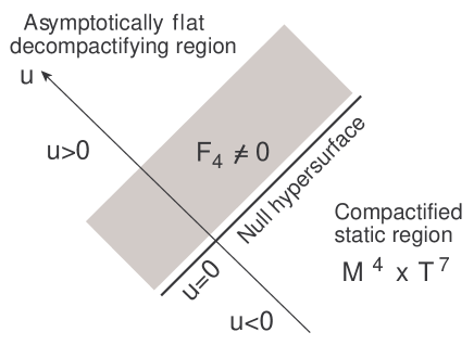
Figure 1: Extension of a decompactifying solution with $m=2$ to a static compactified region across the null hypersurface $u=0$.

From the above results, we can conclude that the compactification in this region is identical to the standard toroidal compactification, apart from a tilt of the extra-dimension direction toward the $\boldsymbol{y}$-direction in the case $\boldsymbol{a}\not=0$. This tilt can be eliminated through a linear coordinate transformation. Further, in terms of the coordinate system $(u,\bar{v},\boldsymbol{y},\bar{\boldsymbol{z}})$, we can extend this compactification to the region $u<0$, as illustrated in Fig. 1. For example, if we assume that the 4-flux vanishes and the spacetime is exactly locally flat there, the action of $g\in\Gamma$ is identical to the simple spatial translation

$$u^{\prime}=u,\quad\bar{v}^{\prime}=\bar{v},\quad\boldsymbol{y}^{\prime}=\boldsymbol{y}+\boldsymbol{a},\quad\bar{\boldsymbol{z}}^{\prime}=\bar{\boldsymbol{z}}-\alpha^{-1}\tilde{\boldsymbol{b}}.$$ (107)

Hence, the compactified spacetime is exactly the product of the $(m+2)$-dimensional Minkowski spacetime and a flat torus $T^{9-m}$ with constant sizes.

Finally, let us examine the regularity of this compactified spacetime in the region $u>0$. For the above parameter choice, $g\in\Gamma$ can be written

$$u^{\prime} = u,$$ (108a)

$$v^{\prime} = v+\frac{1}{2}\tilde{\boldsymbol{b}}\cdot\hat{G}\tilde{\boldsymbol{b}}+\tilde{\boldsymbol{b}}\cdot\boldsymbol{z},$$ (108b)

$$\boldsymbol{y}^{\prime} = \boldsymbol{y}+\boldsymbol{a},$$ (108c)

$$\boldsymbol{z}^{\prime} = \boldsymbol{z}+\hat{G}\tilde{\boldsymbol{b}},$$ (108d)

where

$$\hat{G}^{pq}=(F_{p}-e^{\prime}_{p})\delta_{pq}.$$ (109)

Note that this transformation preserves the quantity

$$v^{\prime}-\frac{1}{2}\boldsymbol{z}^{\prime}\hat{G}^{-1}\boldsymbol{z}^{\prime}=v-\frac{1}{2}\boldsymbol{z}\hat{G}^{-1}\boldsymbol{z}$$ (110)

Because each eigenvalue $\hat{G}_{p}$ of $\hat{G}$ tends to $-\infty$ as $u\rightarrow 0$ and to $\infty$ as $u\rightarrow\infty$, it has to vanish at some value of $u$. On that null hypersurface, $\hat{G}$ becomes singular, and the translations $\hat{G}\tilde{\boldsymbol{b}}_{p}$ in the $z$-space are not linearly independent. If $\boldsymbol{a}=0$, the compactified spacetime has a pathological singularity on this null hypersurface. For example, suppose that $\hat{G}_{1}=0$ at $u=u_{1}$ and $\tilde{b}_{p}^{q}=\delta^{q}_{p}$. Then, each point on the subspace $z^{1}=0$ is a fixed point of the transformation $g$ with $\boldsymbol{a}=\boldsymbol{b}=0,\tilde{\boldsymbol{b}}=\tilde{\boldsymbol{b}}_{1}$. By contrast, in the generic case in which none of $\tilde{\boldsymbol{b}}_{p}$ is annihilated by $\hat{G}$, such a fixed point does not exist. However, we can show that some orbits of $\Gamma$ have accumulation points. In such cases, the quotient spacetime obtained through compactification does not have the Hausdorff property.

These pathological singularities can be avoided if the conditions that $\boldsymbol{a}_{p}$ are generic non-vanishing vectors and different eigenvalues of $\hat{G}$ vanish at different values of $u$ are both satisfied. In this case, the vectors $(\boldsymbol{a}_{p},\tilde{\boldsymbol{b}}_{p})$ ($p=1,\cdots,9-m$) span a $(9-m)$-dimensional subspace of the nine-dimensional $(\boldsymbol{y},\boldsymbol{z})$-space for any value of $u>0$, and the quotient of each $u=\text{const}$ hypersurface is homeomorphic to ${{\mathbb{R}}}^{m+1}\times T^{9-m}$. When one of the eigenvalues of $\hat{G}$ vanishes, some single direction in the $\boldsymbol{z}$-space is decompactified, but simultaneously some direction in the $\boldsymbol{y}$-space is compactified. This implies that the direction of the compactified extra dimensions rotates significantly with $u$ at the point where the matrix $\hat{G}$ becomes singular.

The situation described above is illustrated in Fig. 2. We should first note that the rank of $\hat{G}$ is reduced by at most 1. This implies that if we denote the eigenvalues of $\hat{G}$ by $D_{1}(u),\cdots,D_{9-m}(u)$ and the zero point of each $D_{p}(u)$ by $u_{p}$, then $u_{p}\not=u_{q}$ for $p\not=q$. Suppose that $D_{1}\sim k(u-u_{1})$ near $u=u_{1}$. In the vicinity of $u=u_{1}$, the dimensions $z^{2},...,z^{9-m}$ are toroidally compactified by $\hat{G}\tilde{\boldsymbol{b}}_{2},\cdots,\hat{G}\tilde{\boldsymbol{b}}_{9-m}$, which are mutually independent and nonvanishing, while $y$ and $z^{1}$ are identified by the translation

$$V:\delta y=a,~{}~{}\delta z^{1}=k(u-u_{1}).$$ (111)

If $a=0$, this identification would be only for the direction of $z^{1}$, and the compactification radius would vanish across $u=u_{1}$, as shown in Fig. 2(a). This gives a singular space. However, if $a\neq 0$, the compactification radius does not vanish even for $u=u_{1}$, but the compactification direction rotates in the $z^{1}$-$y$ space, as shown in Fig. 2(b). At $u=u_{1}$, the space decompactifies along the $z^{1}$ direction but compactifies along the $y$ direction, and in this way we can avoid the singularity. Hence, the tilt in the compactification direction leads to a kind of singularity resolution, and $a$ plays the role of a regularisation parameter. It is interesting that the compactification direction is not always the $z^{1}$ direction; rather, it rotates in the direction in which the rank of $\hat{G}$ is reduced. Clearly, this rotation occurs $(9-m)$ times.

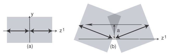
Figure 2: Examples of compactification for (a) $a=0$ and (b) $a\neq 0$. The big arrows indicate the identification, and the shaded regions represent the corresponding fundamental domains.

Thus, starting from a generic light-like solution with two distinct asymptotically flat regions, as in (99), we have constructed a compactified solution that smoothly connects a static region with constant extra dimensions to a dynamical decompactifying region by a light-like 4-form flux. The decompactifying structure in the limit $u\rightarrow\infty$ can be more clearly seen in terms of the coordinates defined by

$$\bar{\bar{v}}=v-\frac{1}{2}\boldsymbol{z}\hat{D}^{-1}\boldsymbol{z},\quad\bar{\bar{\boldsymbol{z}}}=\hat{D}^{-1}\boldsymbol{z},$$ (112)

where $\hat{D}=u+e-e^{\prime}$. In this coordinate system, the spacetime metric for $u\sim\infty$ becomes

$$ds^{2}\approx-2dud\bar{\bar{v}}+d\boldsymbol{y}^{2}+d\bar{\bar{\boldsymbol{z}}}\cdot\hat{D}^{2}d\bar{\bar{\boldsymbol{z}}},$$ (113)

and the transformation $g\in\Gamma$ is written

$$u^{\prime}=u,\quad\bar{\bar{v}}^{\prime}=\bar{\bar{v}},\quad\boldsymbol{y}^{\prime}=\boldsymbol{y}+\boldsymbol{a},\quad\bar{\bar{\boldsymbol{z}}}^{\prime}=\bar{\bar{\boldsymbol{z}}}+\tilde{\boldsymbol{b}}.$$ (114)

This represents a standard toroidal compactification in the $(\boldsymbol{y},\bar{\bar{\boldsymbol{z}}})$-space.

Although we have considered only diagonal solutions here, it is clear from the arguments given to this point that the above construction can be easily extended to light-like solutions with a non-diagonal metric. We also point out that the toroidal compactification considered in the present section preserves 16 supersymmetries of the light-like solution taken as the starting point. This can be explicitly confirmed as follows. First, under the transformation $\Phi$ given in (80), the frame basis $\theta^{a}$ transforms as

$$\Phi^{*}\theta^{-} = \theta^{-},$$ (115a)

$$\Phi^{*}\theta^{+} = \theta^{+}-\frac{1}{2}\boldsymbol{h}^{2}\theta^{-}+h_{I}\theta^{I},$$ (115b)

$$\Phi^{*}\theta^{I} = \theta^{I}-h_{I}\theta^{-},$$ (115c)

where $h_{I}$ is expressed in terms of $(b_{i})=(\boldsymbol{b},\tilde{\boldsymbol{b}})$ as

$$h_{I}=e_{I}^{i}(u)b_{i}.$$ (116)

From the general relation

$$\Phi^{*}\theta^{a}=\Lambda^{a}{}_{b}\theta^{b}\quad\Leftrightarrow\quad S\Gamma^{a}S^{-1}=\Lambda^{a}{}_{b}\Gamma^{b},$$ (117)

the transformation $S$ of the Killing spinor $\epsilon$ is given by

$$S=\exp\left(\tfrac{1}{2}h_{I}\Gamma^{I}\Gamma^{-}\right)=1+\frac{1}{2}h_{I}\Gamma^{I}\Gamma^{-}.$$ (118)

It follows that any spinor field satisfying $\Gamma^{-}\epsilon=0$ is invariant under any transformation of $G_{m}$. Hence, the 16 supersymmetries of the generalised light-like solution studied in §2.2 are preserved under the toroidal compactification considered in the present section.

5 Summary and discussion

In the present paper, we presented a quite general class of spatial-coordinate independent light-like solutions with 16 supersymmetries and studied their toroidal compactification. In particular, starting from a light-like solution which represents the exact Minkowski spacetime in the region $u<0$ and approaches a different Minkowski spacetime as $u\rightarrow\infty$, we constructed a toroidally compactified regular solution whose internal space size is constant for $u<0$ and increases without bound as $u\rightarrow\infty$.

The existence of such a compactification is not a trivial result, because the Einstein equations require that if the 4-form flux $F_{4}$ does not vanish, the spatial metric becomes singular at a finite value of $u$, and as a result, the standard simple toroidal compactification produces singularities. In the present paper, we have overcome this difficulty by considering a tilted toroidal compactification with the help of discrete transformations with boost components. In this compactification, the direction of the compactified extra dimensions rotates several times when we traverse the region with $F_{4}\not=0$ from one flat region to the other flat region.

In the examples constructed in §4, the region with static internal space occupies a half infinite region of spacetime bounded by a null hypersurface. Hence, if we put this region into the region $u<0$, the solution can be regarded as a decompactification transition. However, if we apply the time-reversal operation to this solution, we obtain a solution describing a compactification transition. In either case, two regions always coexist on a fixed time slice. Hence, it is difficult to directly relate the solution to cosmology, even if we ignore the static nature of the base spacetime.

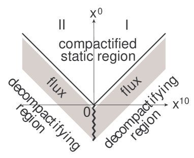
Figure 3: A solution representing the creation and expansion of a static compactified region in an asymptotically decompactifying background.

However, we can construct an interesting solution that may be relevant to cosmology with the following trick. We start from a compactified solution with a static region in the region satisfying $u=(x^{0}-x^{10})/\sqrt{2}>0$. We consider the region satisfying $x^{0}\geq 0$ and $x^{10}\geq 0$ of this solution and refer to it as I. Next, we consider the image of I under the spatial reflection $x^{10}\rightarrow-x^{10}$ and refer to the corresponding new solution in $x^{0}\geq 0$ and $x^{10}\leq 0$ as II. Then, by gluing I and II along $x^{10}=0$, we obtain a smooth compactified solution in the region $x^{0}\geq 0$, because the region $u>0$ of I is a standard toroidal compactification of an exactly flat spacetime (see Fig. 3). In this new solution, the region with a static internal space is given by $x^{0}>|x^{10}|$. Hence, this solution represents the creation of a region with static internal space and its subsequent expansion at the speed of light. When this solution is extended to the region $x^{0}<0$, a singularity appears. However, when quantum effects are taken into account, such a singularity might be avoided, and in that case we would obtain a solution describing the quantum creation of a stable compactified region. It would be quite interesting if a similar solution with spherical symmetry could be found in a class with a time-like Killing spinor.

Finally, we note that the solutions presented in this paper are expected to have a dual description in the matrix theory, which allows a non-perturbative description of cosmological singularities[12, 25]. Indeed, a preliminary study of the solutions indicates that this is possible. It would be interesting to further study the dual description of our solutions and try to understand how the singularity may be tamed and what kind of role the classical singularity resolution by the tilt in the toroidal compactification plays in the dual matrix theory.

Appendix A Exceptional Killing Fields for Diagonal Solutions

In this appendix, we show that the general solution to the Killing equation in the diagonal generalised light-like spacetime is given by (63). We adopt the notation used in §3.2.

Since we are assuming that the case (57b) does not occur, we have

$$\kappa=\text{const},\quad\eta^{u}=d_{0}+\sum_{i\in S_{1}}d_{i}x^{i}.$$ (119)

Hence, for $i,j\in S_{1}$, (48) can be written

$$\partial_{i}\eta^{j}+\partial_{j}\eta^{i}+2(u-u_{0})\partial_{i}\partial_{j}\eta^{v}=0.$$ (120)

This equation is equivalent to the two equations

$$\partial_{i}\eta^{j}+\partial_{j}\eta^{i}=0,$$ (121a)

$$\eta^{v}=\sum_{i\in S_{1}}\eta^{v}_{i}(z)x^{i}+\eta^{v}_{0}(z).$$ (121b)

Here and in the following $z$ represents $(x^{i})_{i\in S_{2}}$.

Next, for $i\in S_{1},\ k\in S_{2}$, (48) reads

$$e^{-2f_{k}}\partial_{k}\eta^{i}+\partial_{i}\eta^{k}+\left((u-u_{0})e^{-2f_{k}}+F_{k}\right)\partial_{i}\partial_{k}\eta^{v}=0.$$ (122)

Differentiation of this equation with respect to $u$ yields

$$\dot{f}_{k}\partial_{k}\eta^{i}-\left\{1-(u-u_{0})\dot{f}_{k}\right\}\partial_{i}\partial_{k}\eta^{v}=0.$$ (123)

Hence, from $K_{k}\not=0$, we obtain

$$\partial_{k}\eta^{i}=0,\quad\partial_{k}\partial_{i}\eta^{v}=0,\quad\partial_{i}\eta^{k}=0.$$ (124)

To summarise, for $i,j\in S_{1}$ we have

$$\eta^{i}=\zeta^{i}(x);\quad\partial_{i}\zeta^{j}+\partial_{j}\zeta^{i}=0,$$ (125)

and for $k\in S_{2}$ we have

$$\eta^{k}=\zeta^{k}(z),\quad\eta^{v}=\sum_{i\in S_{1}}B_{i}x^{i}+\eta^{v}_{0}(z).$$ (126)

Finally, for $k_{1},k_{2}\in S_{2}$, (48) reads

$$e^{2f_{k1}}\partial_{k_{2}}\eta^{k_{1}}+e^{2f_{k2}}\partial_{k_{1}}\eta^{k_{2}}+(e^{2f_{k_{1}}}F^{k_{1}}+e^{2f_{k_{2}}}F^{k_{2}})\partial_{k_{1}}\partial_{k_{2}}\eta^{v}_{0}$$

$$\qquad-2\dot{f}_{k_{1}}e^{2f_{k_{1}}}\delta_{k_{1}\,k_{2}}\left(\kappa u-d_{0}-\sum_{i\in S_{1}}d_{i}x^{i}\right)=0.$$ (127)

If we introduce $\tilde{\zeta}^{k}$ ($k\in S_{2}$) as

$$\tilde{\zeta}^{k}=\eta^{k}+F^{k}\partial_{k}\eta^{v}_{0}-(\kappa u-d_{0})\dot{f}_{k}x^{k},$$ (128)

this equation is equivalent to $d_{i}=0$ [because no other term depends on the coordinates $x^{i}(i\in S_{1}$)] and

$$\partial_{k_{2}}(e^{2f_{k_{1}}}\tilde{\zeta}^{k_{1}})+\partial_{k_{1}}(e^{2f_{k_{2}}}\tilde{\zeta}^{k_{2}})=0,$$ (129)

which is the Killing equation for the Euclidean space. Hence, we obtain

$$\eta^{k}+F^{k}\partial_{k}\eta^{v}_{0}-(u\kappa-d_{0})\dot{f}_{k}x^{k}=\sum_{l\in S_{2}}e^{f_{l}-f_{k}}\omega_{kl}(u)x^{l}+\tilde{a}^{k}(u),$$ (130)

where $\omega_{kl}=-\omega_{lk}$. Differentiating both sides of this equation with respect to $u$, we have

$$\partial_{k}\eta^{v}_{0}=2\ell_{k}x^{k}+2\sum_{l\in S_{2}}S_{kl}x^{l}+a_{k},$$ (131)

where

$$2\ell_{k}:=e^{2f_{k}}{{\left[(\kappa u-d_{0})\dot{f}_{k}\right]}^{\hbox{.}}},$$ (132a)

$$2S_{kl}:=e^{f_{k}+f_{l}}\left\{\dot{\omega}_{kl}-(\dot{f}_{k}-\dot{f}_{l})\omega_{kl}\right\},$$ (132b)

$$a_{k}=e^{2f_{k}}{{(\tilde{a}^{k})}^{\hbox{.}}}.$$ (132c)

Since $\eta^{v}_{0}$ depends only on $z=(x^{k})_{k\in S_{2}}$, $\ell_{k},S_{kl}$ and $a_{k}$ must be constant. Further, the integrability of $\partial_{k}\eta^{v}_{0}$ requires $S_{kl}=S_{lk}$. Therefore, we obtain

$$\dot{\omega}_{kl}=0,$$ (133)

$$S_{kl}=-s_{kl}\omega_{kl};\quad 2s_{kl}:=e^{f_{k}+f_{l}}(\dot{f}_{k}-\dot{f}_{l}).$$ (134)

To summarise, we have

$$\eta^{k}=\sum_{l\in S_{2}}\left(e^{-f_{k}+f_{l}}+2s_{kl}F^{k}\right)\omega_{kl}x^{l}+e_{k}x^{k}+A_{k},$$ (135a)

$$\eta^{v}_{0}=C+\sum_{k\in S_{2}}\left(B_{k}x^{k}+\ell_{k}(x^{k})^{2}\right)-\sum_{k,l\in S_{2}}s_{kl}\omega_{kl}x^{k}x^{l},$$ (135b)

where

$$e_{k}=(\kappa u_{0}-d_{0})\dot{f}_{k}(u_{0}).$$ (136)

Here, since both $S_{kl}$ and $\omega_{kl}$ are constant, the relation $\omega_{kl}\not=0$ holds only when $s_{kl}=-s_{lk}$ is constant. Inserting these expressions into (45), we obtain the result, (63).

References

• [1] Gibbons,Β G., LΓΌ,Β H. and Pope,Β C.: Brane Worlds in Collision, Phys. Rev. Lett. 94, 131602 (2005).
• [2] Kodama,Β H. and Uzawa,Β K.: Moduli Instability in Warped Compactifications of the Type IIB Supergravity, JHEP 0507, 061 (2005).
• [3] Kodama,Β H. and Uzawa,Β K.: Comments on the four-dimensional effective theory for warped compactification, JHEP 0603, 053 (2006).
• [4] Candelas,Β P., Green,Β P. and Hubsch,Β T.: Finite distance between distinct Calabi-Yau manifolds, Phys. Rev. Lett. 62, 1956–1959 (1989).
• [5] Greene,Β B.Β R.: String Theory on Calabi-Yau Manifolds: Lectures at the TASI-96 summer school on Strings, Fields and Duality, hep-th/9702155 (1997).
• [6] BrΓ€ndle,Β M. and Lukas,Β A.: Flop Transitions in M-theory Cosmology, Phys. Rev. D 68, 024030 (2003).
• [7] JΓ€rv,Β L., Mohaupt,Β T. and Saueressig,Β F.: Effective supergravity actions for flop transitions, JHEP 0312, 047 (2003).
• [8] Lukas,Β A., Palti,Β E. and Saffin,Β P.: Type IIB Conifold Transitions in Cosmology, Phys. Rev. D 71, 066001 (2005).
• [9] Mohaupt,Β T. and Saueressig,Β F.: Effective supergravity actions for conifold transitions, JCAP 0501, 006 (2005).
• [10] Mohaupt,Β T. and Saueressig,Β F.: Conifold cosmologies in IIA string theory, Fortsch. Phys. 53, 522-527 (2005).
• [11] Liu, H., Moore, G.Β W., and Seiberg, N.: Strings in a time-dependent orbifold, JHEP 0206, 045 (2002); Strings in time-dependent orbifolds, JHEP 0210, 031 (2002).
• [12] Craps,Β B., Sethi,Β S. and Verlinde,Β E.: A Matrix Big Bang, JHEP 0510, 005 (2005).
• [13] Li, M.: A class of cosmological matrix models, Phys.Β Lett.Β B 626, 202 (2005).
• [14] Hikida, Y., Nayak, R. R. and Panigrahi, K. L.: D-branes in a big bang / big crunch universe: Misner space, JHEP 0509, 023 (2005).
• [15] Chen,Β B.: The Time-dependent Supersymmetric Configurations in M-theory and Matrix Models, Phys. Lett. B 632, 393–398 (2005).
• [16] Ishino,Β T., Kodama,Β H. and Ohta,Β N.: Time-dependent Solutions with Null Killing Spinor in M-theory and Superstrings, Phys. Lett. B 631, 68–73 (2005).
• [17] Robbins, D. and Sethi, S.: A matrix model for the null-brane, JHEP 0602, 052 (2006).
• [18] She, J.Β H.: Winding string condensation and noncommutative deformation of spacelike singularity, hep-th/0512299.
• [19] Craps, B., Rajaraman, A. and Sethi, S.: Effective dynamics of the matrix big bang, Phys.Β Rev.Β D 73, 106005 (2006).
• [20] Chu, C.Β S., and Ho, P.Β M.: Time-dependent AdS/CFT duality and null singularity, JHEP 0604, 013 (2006).
• [21] Das, S.Β R. and Michelson, J.: pp wave big bangs: Matrix strings and shrinking fuzzy spheres, Phys. Rev. D 72, 086005 (2005); Matrix membrane big bangs and D-brane production, Phys.Β Rev.Β D 73, 126006 (2006). Das, S.Β R., Michelson, J., Narayan, K. and Trivedi, S.Β P.: Time dependent cosmologies and their duals, Phys.Β Rev.Β D 74, 026002 (2006).
• [22] Lin, F.Β L. and Wen, W.Β Y.: Supersymmetric null-like holographic cosmologies, JHEP 0605, 013 (2006).
• [23] Martinec, E.Β J., Robbins, D. and Sethi, S.: Toward the end of time, hep-th/0603104.
• [24] Chen,Β H.-Z. and Chen,Β B.: Matrix model in a class of time dependent supersymmetric backgrounds, Phys.Β Lett.Β B 638, 74–79 (2006).
• [25] Ishino,Β T. and Ohta,Β N.: Matrix String Description of Cosmic Singularities in a Class of Time-dependent Solutions, Phys. Lett. B 638, 105–109 (2006).
• [26] Tod,Β K.Β P.: All metrics admitting supercovariantly constant spinors, Phys. Lett. B 121, 241–244 (1983).
• [27] Tod,Β K.: More on supercovariantly constant spinors, Class. Quantum Grav. 11, 1801–1820 (1995).
• [28] Gauntlett,Β J., Gutowski,Β J., Hull,Β C., Pakis,Β S. and Reall,Β H.: All supersymmetric solutions of minimal supergravity in five dimensions, Class. Quant. Grav. 20, 4587–4634 (2003).
• [29] Gauntlett,Β J. and Gutowski,Β J.: All supersymmetric solutions of minimal gauged supergravity in five dimensions, Phys. Rev. D 68, 105009 (2003).
• [30] Gauntlett,Β J. and Pakis,Β S.: The Geometry of D=11 Killing Spinors, JHEP 0304, 039 (2003).
• [31] Gauntlett,Β J., Gutowski,Β J. and Pakis,Β S.: The Geometry of $D=11$ Null Killing Spinors, JHEP 0312, 049 (2003).
• [32] Hackett-Jones,Β E. and Smith,Β D.: Type IIB Killing spinors and calibrations, JHEP 0411, 029 (2004).
• [33] Gran,Β U., Gutowski,Β J. and Papadopoulos,Β G.: The spinorial geometry of supersymmetric IIB backgrounds, Class. Quant. Grav. 22, 2453–2492 (2005).
• [34] Kowalski-Glikman,Β J.: Vacuum states in supersymmetric Kaluza-Klein theory, Phys. Lett. B 134, 194 (1984).
• [35] Kodama,Β H.: Canonical Structure of Locally Homogeneous Systems on Compact Closed 3-Manifolds of Types $E^{3}$, Nil and Sol, Prog. Theor. Phys. 99, 173–236 (1998).
• [36] Kodama,Β H.: Phase Space of Compact Bianchi Models with Fluid, Prog. Theor. Phys. 107, 305–362 (2002).