We study the semiclassical fluctuation problem around bounce solutions for a self-interacting scalar field in curved space. As in flat space, the fluctuation problem separates into partial waves labeled by an integer $l$, and we determine the large $l$ behavior of the fluctuation determinants, a quantity needed to define a finite fluctuation prefactor. We also show that while the Coleman-De Luccia bounce solution has a single negative mode in the $l=0$ sector, the oscillating bounce solutions also have negative modes in partial waves higher than the s-wave, further evidence that they are not directly related to quantum tunneling.

I Introduction

The problem of false vacuum decay in the presence of gravity cdl provides an important window into the behavior of interacting quantum fields in curved space-time, and is also important for our understanding of string theory and quantum gravity banks ; kachru ; bousso1 , and inflationary models of cosmology linde . Since the pioneering work of Coleman and De Luccia cdl , much has been learned regarding the existence and properties of bounce solutions for interacting scalar fields coupled to gravity hm ; jensen ; mottola ; parke ; kimyeong ; samuel ; banks ; demetrian ; hw ; bousso ; banksjohnson , and consequently the exponential factor in the false vacuum decay rate. On the other hand, relatively little is known about the prefactor in the decay rate. This is in distinct contrast to the flat space case where the entire computation is well understood physically and mathematically; analytically in the thin-wall limit langer ; voloshin ; stone ; coleman1 ; voloshin2 , and numerically in general konoplich ; strumia ; baacke ; dunnemin . Here we begin to address this prefactor question with coupling to gravity by studying the problem of quantum fluctuations about the bounce solutions. A full solution to this problem is not possible at present for the simple reason that computing the renormalized fluctuation prefactor would require an understanding of the renormalization of quantum gravity. However, we argue that certain interesting things can be learned, in particular in the limit where the gravitational background is fixed to be de Sitter space.

In the flat space false vacuum decay problem, the fluctuation operator separates into partial waves labeled by an integer $l$, and there are three important types of modes. In the $l=0$ sector there is a single negative mode and this is responsible for the decaying nature of the problem langer ; voloshin ; stone ; coleman1 . In the $l=1$ sector there are four zero modes corresponding to translational invariance in four-dimensional Euclidean space, and these zero modes lead to collective coordinate contributions to the overall fluctuation determinant. For $l\geq 2$ the eigenvalues are all positive, and since for each $l$ the fluctuation operator is a one-dimensional radial operator, one can compute the determinant straightforwardly using the Gel’fand-Yaglom method (described below in Section IV). Formally, the determinant of the full fluctuation operator is a product of the determinants for all $l$, including degeneracies, so the large $l$ behavior is crucial for defining a finite renormalized fluctuation determinant. In the thin-wall limit, where the energy gap between the true and false vacua is small, the computation can essentially be done analytically langer ; voloshin ; stone ; coleman1 , and one has a beautiful physical picture of this process as nucleation of bubbles. Away from the thin-wall limit, the computation can be done by various approximate or numerical approaches konoplich ; strumia ; baacke ; dunnemin . Our main motivation here is to investigate how the behavior of the fluctuation operator is affected by the inclusion of coupling to gravity.

With the inclusion of gravity, Coleman and De Luccia argued cdl that the bounce solutions are still radially symmetric (although this has not been rigorously proved, as it has been in flat space coleman2 ). Interestingly, new classes of bounce solutions arise, with different physical interpretations. The Coleman-De Luccia (CDL) bounce generalizes the flat space bounce and is presumed to be associated with quantum tunneling cdl . There also exists the Hawking-Moss (HM) bounce hm which is interpreted physically in terms of a thermal transition linde ; hw . More recently it has been shown that there are also “oscillating bounce” solutions in which the scalar field passes over the barrier more than once banksjohnson ; bousso ; demetrian ; hw . As emphasized in hw , these oscillating bounces interpolate between the CDL and HM bounces, and reflect the thermal character of quantum field theory in de Sitter space. Since all these bounces are radial, a similar separation of the fluctuation problem into “partial waves” is possible, with the physically plausible assumption that such radial fluctuations dominate. But even with this separation, the fluctuation problem is still considerably more subtle with the inclusion of gravity, as it requires a detailed constraint analysis to disentangle the physical fluctuation fields. Here we consider the scalar fluctuations in the formalism developed in turok1 ; turok2 ; lav1 ; lav2 . The existence of negative modes in the $l=0$ sector for these scalar fluctuations has been investigated in turok1 ; turok2 ; lav1 ; lav2 . We extend this fluctuation analysis in several ways by considering the behavior for higher $l$. We study two main questions: First, we investigate the large $l$ behavior of the fluctuation determinants within each partial wave sector. We find an explicit expression for the leading large $l$ behavior, and a numerically accurate estimate for the subleading behavior. Second, we analyze the existence of negative modes not just in the $l=0$ sector, but also for higher $l$, and show that the oscillating bounce solutions have negative modes for higher $l$. This is further evidence for the physical picture in hw that these oscillating bounces are not directly related to quantum tunneling, but rather reflect the thermal nature of quantum field theory in de Sitter space. We are not able to study the $l=1$ sector, as this fluctuation formalism does not apply here turok1 ; turok2 , and so this requires a separate study.

In Section II we review the model and the construction of bounce solutions to the classical equations of motion. In Section III we summarize the scalar fluctuation problem to be studied. Section IV is devoted to the study of the large $l$ behavior of the fluctuation determinant, in which we review the flat space approach. In Section V we count the negative modes for various $l$ for fluctuations about bounce solutions. Section VI contains our conclusions and an Appendix gives the relation of our fluctuation operator to other forms considered in the literature.

II Classical bounce solutions

Before discussing quantum fluctuations, we briefly review the derivation of the bounce solutions themselves. We consider the four dimensional self-interacting scalar field system with Euclidean action

$$S_{E}=\int d^{4}x\sqrt{g}\left[\frac{1}{2}\nabla_{\mu}\phi\nabla^{\mu}\phi+V(\phi)-\frac{1}{2\kappa}R\right]\quad,$$ (2.1)

where the gravitational coupling is expressed as $\kappa=8\pi/M_{\rm pl}^{2}$. In terms of the proper time $\sigma$, the metric has the form

$$ds^{2}=d\sigma^{2}+a^{2}(\sigma)d\Omega_{3}^{2}\quad.$$ (2.2)

The classical Euclidean equations of motion are

$$\ddot{\phi}+3\frac{\dot{a}}{a}\dot{\phi}-V^{\prime}(\phi) = 0\quad,$$ (2.3)

$$\dot{a}^{2}-\frac{\kappa a^{2}}{3}\left[\frac{1}{2}\dot{\phi}^{2}-V(\phi)\right] = K\quad,$$ (2.4)

where the overdot denotes $\frac{d}{d\sigma}$, and $V^{\prime}(\phi)\equiv\frac{\delta V(\phi)}{\delta\phi}$. $K=0,\pm 1$ corresponding to flat, closed/open universes, respectively. The boundary conditions for the bounce solutions are

$$\dot{\phi}(0)=0\quad, \dot{\phi}(\sigma_{\rm max})=0\quad,$$

$$a(0)=0\quad, a(\sigma_{\rm max})=0\quad,$$ (2.5)

where $\sigma_{\rm max}$ is defined by the last equation: $a(\sigma_{\rm max})=0$. In this paper we consider $K=1$, which leads to the normalization condition

$$\dot{a}(0)=1\quad.$$ (2.6)

We choose the standard quartic scalar field potential hw ; banksjohnson :

$$V(\phi) = V_{\rm top}+\beta H_{\rm top}^{2}v^{2}\left[-\frac{1}{2}\left(\frac{\phi}{v}\right)^{2}-\frac{b}{3}\left(\frac{\phi}{v}\right)^{3}+\frac{1}{4}\left(\frac{\phi}{v}\right)^{4}\right]$$ (2.7)

$$\equiv \beta H_{\rm top}^{2}v^{2}\left[\frac{1}{\beta\epsilon^{2}}+f\left(\frac{\phi}{v}\right)\right]\quad,$$

which is sketched in Figure 1. The function $f$ is a function of the dimensionless field $\varphi\equiv\frac{\phi}{v}$:

$$f(\varphi)\equiv-\frac{1}{2}\varphi^{2}-\frac{b}{3}\varphi^{3}+\frac{1}{4}\varphi^{4}\quad.$$ (2.8)

The potential $V(\phi)$ has two local minima, a false vacuum $\phi_{\rm fv}$, and a true vacuum $\phi_{\rm tv}$, separated by a local maximum $\phi_{\rm top}$, chosen to be at $\phi_{\rm top}=0$. A crucial difference between the flat-space case and the gravitational case is that the overall constant $V_{\rm top}$ in the potential is now significant, as it plays the role of a cosmological constant cdl . A corresponding mass scale is defined as

$$H_{\rm top}\equiv\sqrt{\frac{\kappa V_{\rm top}}{3}}=\sqrt{\frac{8\pi V_{\rm top}}{3M_{\rm pl}^{2}}}\quad.$$ (2.9)

The dimensionless parameter $\beta$ in (2.7) characterizes the ratio of the barrier curvature (at $\phi_{\rm top}=0$) to $H_{\rm top}^{2}$

$$\beta\equiv\frac{|V^{\prime\prime}(0)|}{H_{\rm top}^{2}}\quad,$$ (2.10)

and is an important quantity in determining the existence and form of bounce solutions cdl ; mottola ; jensen ; demetrian ; hw . Another useful dimensionless quantity is the ratio of the field scale $v$ to the Planck mass $M_{\rm pl}$:

$$\epsilon\equiv\sqrt{\frac{8\pi v^{2}}{3M_{\rm pl}^{2}}}=\sqrt{\frac{\kappa v^{2}}{3}}\quad,$$ (2.11)

and we consider here values such that the potential is everywhere positive.

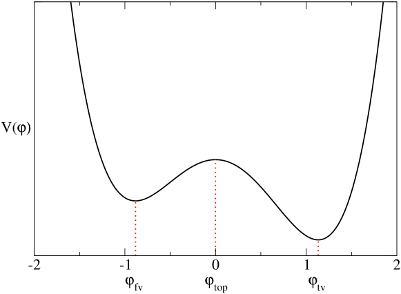
Figure 1: The scalar field potential $V(\varphi)$ with the parameters: $\beta=45$, $b=0.25$, $\epsilon=0.23$.

The three critical points of $V(\phi)$ correspond to three trivial solutions to the bounce equations (2.3) - (2.6), in which $\phi$ is constant at one of these critical values $\phi_{c}$ such that $V^{\prime}(\phi_{c})=0$:

$$\phi(\sigma) = \phi_{c}$$

$$a(\sigma) = \frac{1}{H}\,\sin(H\sigma)\quad.$$ (2.12)

The three solutions of this form are : (i) the false vacuum constant solution with $\phi=\phi_{\rm fv}$, and $H_{\rm fv}\equiv\sqrt{\kappa V(\phi_{\rm fv})/3}$; (ii) the true vacuum constant solution with $\phi=\phi_{\rm tv}$, and $H_{\rm tv}\equiv\sqrt{\kappa V(\phi_{\rm tv})/3}$; (iii) the Hawking-Moss hm solution with $\phi=\phi_{\rm top}=0$, and $H_{\rm top}$ given by (2.9).

More interesting are the bounce solutions in which $\phi$ is not constant. For definiteness, we restrict our attention to bounces beginning near the true vacuum and ending near the false vacuum:

$$\phi(0)\approx\phi_{\rm tv}\quad, \phi(\sigma_{\rm max})\approx\phi_{\rm fv}\quad.$$ (2.13)

Other bounces exist demetrian ; hw and can be treated with completely analogous methods. Bounces can be labeled by an integer $n$ characterizing how many times they cross the barrier. We will refer to the Coleman-De Luccia bounce cdl as a “single bounce” solution, and the $n\geq 2$ bounces will be termed “oscillating bounces” hw . In the flat space limit, only single bounce solutions have finite action. The explicit bounce solutions can be found numerically by a straightforward shooting technique, as follows.

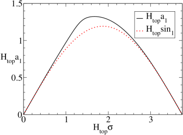
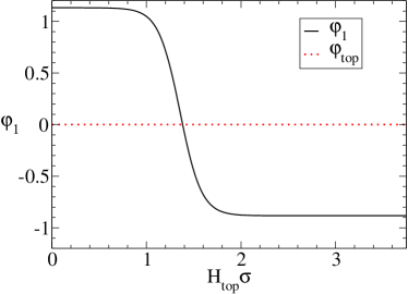
Figure 2: Single bounce solution to (2.3)-(2.6), for parameter values: $\beta=45$, $b=0.25$, $\epsilon=0.23$. The shooting procedure determines the initial scalar field value $\varphi_{1}(0)=\varphi_{\rm fv}-0.000\,145\,223\,243\,267\,576\,9$, and $\sigma_{\rm max}$ is given by: $H_{\rm top}\sigma_{\rm max}^{\rm 1b}=3.7475$. Here $\sin_{1}\equiv\frac{1}{H_{1}}\sin\left(H_{1}\sigma\right)$, and $H_{1}\equiv\pi/\sigma_{\rm max}^{\rm 1b}$.

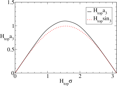
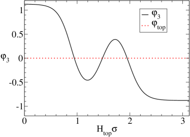
Figure 3: Triple bounce solution to (2.3)-(2.6), for parameter values: $\beta=45$, $b=0.25$, $\epsilon=0.23$. The shooting procedure determines the initial scalar field value $\varphi_{3}(0)=\varphi_{\rm tv}-0.008\,860\,088\,903\,713\,227$, $H_{\rm top}\sigma_{\rm max}^{\rm 3b}=3.1243$. Here $\sin_{3}\equiv\frac{1}{H_{3}}\sin\left(H_{3}\sigma\right)$, and $\sigma_{\rm max}$ is given by: $H_{3}\equiv\pi/\sigma_{\rm max}^{\rm 3b}$.

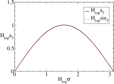
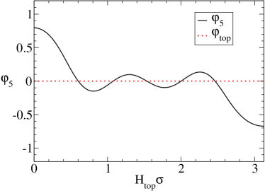
Figure 4: Quintuple bounce solution to (2.3)-(2.6), for parameter values: $\beta=45$, $b=0.25$, $\epsilon=0.23$. The shooting procedure determines the initial scalar field value $\varphi_{5}(0)=\varphi_{\rm tv}-0.337\,102\,748\,195\,264\,1$, $H_{\rm top}\sigma_{\rm max}^{\rm 5b}=3.1264$. Here $\sin_{5}\equiv\frac{1}{H_{5}}\sin\left(H_{5}\sigma\right)$, and $\sigma_{\rm max}$ is given by: $H_{5}\equiv\pi/\sigma_{\rm max}^{\rm 5b}$.

The shooting parameter is the initial value $\phi(0)$ of the scalar field. This value is chosen near the true vacuum value and adjusted until the coupled initial value problem (2.3) - (2.6) has a solution satisfying both $a(\sigma_{\rm max})=0$ and $\dot{\phi}(\sigma_{\rm max})=0$, for some $\sigma_{\rm max}$. The value of $\sigma_{\rm max}$ is determined by this shooting procedure, and so depends on the bounce. Since the metric field behaves as $a(\sigma)\sim\sigma$ for small $\sigma$, we cannot directly start integrating (2.3) at $\sigma=0$. Instead, we Taylor expand both $a(\sigma)$ and $\phi(\sigma)$ about $0$, and use these Taylor expansions to begin the integration at a point very close to $0$. We then do a shooting scan of $\phi(0)$, adjusting it digit by digit, in a rational form to preserve precision. This computation is simple to implement in Mathematica. In a few minutes one can determine $\phi(0)$ to 32 decimal places. We found that the shooting went faster with the following simple rescaling of the differential equations, as in banksjohnson : we rescale $\varphi=\phi/v$, and $\sigma$ and $a(\sigma)$ as: $s=\sqrt{\beta H_{\rm top}^{2}}\,\sigma$, and $\rho(s)=\sqrt{\beta H_{\rm top}^{2}}\,a(\sigma)$, so that the parameters $v$ and $H_{\rm top}$ scale out of the classical equations of motion.

Representative examples of bounce solutions with $\phi(0)\approx\phi_{\rm tv}$ and $\phi(\sigma_{\rm max})\approx\phi_{\rm fv}$ are shown in Figures 2, 3 and 4. These plots are for $\beta=45$. For larger $\beta$ more oscillations are possible in the bounce solutions. Note that the metric field $a(\sigma)$ deviates significantly from the sinusoidal form of (2.12) for the single and triple bounce, but less so for the quintuple bounce. This, together with the fact that the scalar field $\phi$ is closer to the Hawking-Moss constant value of $\phi_{\rm top}=0$, is another reflection of the fact that the highly oscillating bounce solutions tend towards the Hawking-Moss solution hw .

III Fluctuation operator

Having reviewed how to find the classical bounce solutions, we now turn to the problem of fluctuations about these solutions. With the inclusion of gravity, the fluctuation problem becomes more subtle, and the fluctuation operator about such cosmological instantons has been widely studied tanaka ; turok1 ; turok2 ; lav1 ; lav2 . The variation of the action under fluctuations of the scalar field and the metric field requires a nontrivial constraint analysis, with different possible gauge fixing procedures. For the purpose of this paper, we choose the gauge fixing scheme described in Section 4.3 of lav2 , and Section IV of turok2 . In this scheme, the only physical degree of freedom is the fluctuation of the scalar field, and the second variation of the action can be expressed as (compare with Eqn. (12) in turok2 and Eqn. (18) in the second reference of lav3 ):

$$S^{(2)}[\delta\phi]=\pi^{2}\int d\sigma\,\delta\phi\left\{-\frac{d}{d\sigma}\left(\frac{a^{3}(\sigma)}{{\mathcal{Q}}(\sigma)}\frac{d}{d\sigma}+a^{3}(\sigma)U[a(\sigma),\phi(\sigma)]\right)\right\}\delta\phi\quad.$$ (3.14)

Here

$${\mathcal{Q}}(\sigma)\equiv 1+\frac{\kappa a^{2}(\sigma)\dot{\phi}^{2}(\sigma)}{2(-\Delta_{3}-3K)}\quad,$$ (3.15)

and

$$U[a,\phi] \equiv \frac{1}{{\mathcal{Q}}}V^{\prime\prime}(\phi)+\frac{-\Delta_{3}}{{\mathcal{Q}}a^{2}}+\kappa\left\{\frac{2\dot{\phi}^{2}}{{\mathcal{Q}}}+\frac{-a^{2}\left[V^{\prime}(\phi)\right]^{2}+5a\dot{a}\dot{\phi}V^{\prime}(\phi)-6\dot{a}^{2}\dot{\phi}^{2}}{{\mathcal{Q}}^{2}(-\Delta_{3}-3K)}\right\}\quad.$$ (3.16)

Here we have temporarily re-instated the $K$ dependence, although in our numerical studies we return to $K=1$, and $\Delta_{3}$ is the Laplacian on $S^{3}$.

To pass from this secondary action to the Jacobi equation morse , a Sturm-Liouville differential equation whose eigenvalues will define the determinant of the fluctuation operator, we need to specify the weight function. The weight function is determined by defining

$$||\delta\phi||^{2}\equiv\int d^{4}x\sqrt{g}\left(\delta\phi\right)^{2}=2\pi^{2}\int d\sigma\,a^{3}(\sigma)\left[\delta\phi(\sigma)\right]^{2}$$ (3.17)

Then in terms of the perturbation function $\Phi\equiv\delta\phi$, the fluctuation equation (the Jacobi equation morse ) is

$$-\frac{1}{a^{3}}\frac{d}{d\sigma}\left(\frac{a^{3}}{{\mathcal{Q}}}\frac{d\Phi}{d\sigma}\right)+U[a,\phi]\Phi=\lambda\Phi\quad,$$ (3.18)

which is defined on the interval $\sigma\in[0,\sigma_{\rm max}]$, with Dirichlet boundary conditions, and where $\lambda$ denotes the eigenvalue. The “fluctuation potential” $U[a,\phi]$ is the function in (3.16). The $S^{3}$ Laplacian $\Delta_{3}$ appearing in (3.15) and (3.16) can be replaced by its eigenvalue: $-\Delta_{3}\to l(l+2)$, so we obtain a fluctuation equation as an ordinary differential equation for each integer value of $l$ ($l\neq 1$).

In the flat space limit, $\kappa\to 0$, ${\mathcal{Q}}\to 1$, $a\to\sigma$, and $\sigma_{\rm max}\to\infty$; in which case we recover the familiar flat space fluctuation equation coleman1

$$-\frac{1}{r^{3}}\frac{d}{dr}\left(r^{3}\,\frac{d\Phi}{dr}\right)+U[\phi(r)]\Phi=\lambda\Phi\quad,$$

$$U[\phi]=V^{\prime\prime}(\phi)+\frac{l(l+2)}{r^{2}}\quad,$$ (3.19)

where $\sigma$ becomes identified with the Euclidean length $r$, which ranges from $0$ to $\infty$. Much is known about solutions to this flat space fluctuation equation (3.19). Our goal now is to study some properties of the more general fluctuation equation in (3.18).

For completeness, we note here that for the purposes of discussing the existence of negative modes it is possible to make other choices of the weight function, which yield superficially different-looking Jacobi operators. In Appendix A we give the explicit transformation between our choice (3.17) of weight function and those made in turok1 ; turok2 ; lav1 ; lav2 ; lav3 .

IV Large $l$ behavior of fluctuation determinants

Both $\phi(\sigma)$ and $a(\sigma)$ are functions just of the proper time $\sigma$, so the fluctuation problem separates into partial waves, which can be labeled by an integer $l$, just as in the flat space case. Then formally we can write the log determinant of the fluctuation operator $\Lambda$ as

$$\ln\left(\frac{\mbox{Det}\left[\Lambda\right]}{\mbox{Det}\left[\Lambda_{\rm free}\right]}\right)=\sum_{l}^{\infty}(l+1)^{2}\ln\left(\frac{\mbox{Det}\left[\Lambda^{(l)}\right]}{\mbox{Det}\left[\Lambda^{(l)}_{\rm free}\right]}\right)\qquad({\rm formal~{}!})\quad,$$ (4.20)

where $\Lambda^{(l)}$ is the differential operator in (3.18), for each $l$, and the eigenvalue of $-\Delta_{3}$ is $l(l+2)$, with degeneracy $(l+1)^{2}$. This formal expression (4.20) must be interpreted with caution, because as in the flat space case, for low $l$ values there may be negative and zero modes. Nevertheless, for generic $l$, since each $\Lambda^{(l)}$ is a one-dimensional differential operator, the determinant ratio $\left(\mbox{Det}\left[\Lambda^{(l)}\right]/{\mbox{Det}\left[\Lambda^{(l)}_{\rm free}\right]}\right)$ is finite, and can be computed efficiently using the Gel’fand-Yaglom technique gy ; levit ; forman ; kirsten ; kleinert . In this approach one simply numerically integrates both Jacobi equations, $\Lambda^{(l)}\,\Phi^{(l)}=0$ and $\Lambda^{(l)}_{\rm free}\,\Phi_{\rm free}^{(l)}=0$, for zero eigenvalue and with suitable common initial value boundary conditions, $\Phi^{(l)}(\sigma)\sim\sigma^{l}$ at $\sigma=0$. Then the ratio of the determinants is the ratio of these two functions evaluated at $\sigma_{\rm max}$:

$$\frac{\mbox{Det}\left[\Lambda^{(l)}\right]}{\mbox{Det}\left[\Lambda^{(l)}_{\rm free}\right]}=\frac{\Phi^{(l)}(\sigma_{\rm max})}{\Phi^{(l)}_{\rm free}(\sigma_{\rm max})}\quad.$$ (4.21)

This technique provides a simple computational method for evaluating the finite determinant for each $l$, without ever having to compute any eigenvalues. However, of course, even though each term on the RHS of (4.20) is finite, the sum over $l$ diverges forman . This is clearly because we have not regularized and renormalized the determinant. This divergence is not a feature of the gravitational coupling — exactly the same thing happens in flat space baacke ; dunnemin , where one can indeed extract a finite renormalized determinant by subtracting certain known contributions from $\ln\left(\mbox{Det}\left[\Lambda^{(l)}\right]/{\mbox{Det}\left[\Lambda^{(l)}_{\rm free}\right]}\right)$ for each $l$, rendering the sum finite. The precise form of the subtractions can be found in various ways, using Feynman diagram techniques baacke , zeta function regularization kirsten , or radial WKB dunnemin . The finite part of these subtractions is related to the specific renormalization prescription strumia ; baacke ; dunnemin ; dhlm ; burnier . In dunnemin , in flat space, it was checked explicitly that the result of this procedure connects smoothly to the analytic thin-wall limit results for the renormalized fluctuation determinant.

A key element of this approach is knowledge of the large $l$ behavior of $\ln\left(\mbox{Det}\left[\Lambda^{(l)}\right]/{\mbox{Det}\left[\Lambda^{(l)}_{\rm free}\right]}\right)$, which must be subtracted to make the $l$ sum finite (renormalization involves a further step). In flat space the radial WKB analysis leads to the following expression for the large $l$ behavior dunnemin :

$$\ln\left(\frac{\mbox{Det}\left[\Lambda^{(l)}\right]}{\mbox{Det}\left[\Lambda^{(l)}_{\rm free}\right]}\right)\sim\frac{\frac{1}{2}\int_{0}^{\infty}dr\,r\,W}{(l+1)}-\frac{\frac{1}{8}\int_{0}^{\infty}dr\,r^{3}\,W(W+2V^{\prime\prime}[\phi_{\rm fv}])}{(l+1)^{3}}+O\left(\frac{1}{(l+1)^{5}}\right)\quad,\qquad l\to\infty\quad.$$ (4.22)

Here $W=V^{\prime\prime}[\phi]-V^{\prime\prime}[\phi_{\rm fv}]$. Subtracting these terms makes the sum over $l$ in (4.20) finite, and is one part of the analysis leading to a finite renormalized fluctuation determinant. We now turn our attention to the large $l$ behavior of these determinants in the gravitational case.

It is immediately clear that with gravitational coupling such a computation cannot be done for the renormalized fluctuation determinant, as we do not know how to renormalize gravity. Nevertheless, we can study this question in the de Sitter limit, where the gravitational background is fixed to be of the de Sitter form in (2.12). This limit is physically appropriate when the variation of the potential on the scale of the barrier is much less than $V_{\rm top}$ rubakov . For the moderate values of the cubic coupling $b$ in (2.7) considered here, this amounts to the condition $\beta\epsilon^{2}\ll 1$, which means that the potential is large and positive, with:

$$H_{\rm fv}\approx H_{\rm top}\approx H_{\rm tv}\approx H\quad.$$ (4.23)

Thus, fixing the metric to have the de Sitter form

$$a(\sigma)=\frac{1}{H}\sin\left(H\sigma\right)\quad,$$ (4.24)

the classical equations of motion reduce to a single equation for $\phi(\sigma)$:

$$\ddot{\phi}+3\frac{\dot{a}}{a}\dot{\phi}-V^{\prime}(\phi)=0\quad.$$ (4.25)

Even though $a(\sigma)$ is determined, one still finds various different types of oscillating bounce solutions for $\phi(\sigma)$, as described in the previous section. These have been extensively studied recently in hw with a different choice of parameter $\beta=70.03$.

To compute the determinant ratio in (4.21), consider first the false vacuum case, which is the appropriate “free” reference operator: $\Lambda^{(l)}_{\rm free}=\Lambda^{(l)}_{\rm fv}$. Since $\phi=\phi_{\rm fv}$ is constant, and $V^{\prime}(\phi_{\rm fv})$ vanishes, the fluctuation potential (3.16) simplifies dramatically, and the Jacobi equation (3.18) for zero eigenvalue becomes

$$-\ddot{\Phi}_{\rm fv}^{(l)}-3\frac{\dot{a}}{a}\dot{\Phi}_{\rm fv}^{(l)}+\left[V^{\prime\prime}(\phi_{\rm fv})+\frac{l(l+2)}{a^{2}}\right]\Phi_{\rm fv}^{(l)}=0\quad,$$ (4.26)

with $a(\sigma)=\frac{1}{H_{\rm fv}}\sin(H_{\rm fv}\sigma)$. The zero mode solution with the correct initial value behavior, $\Phi_{\rm fv}^{(l)}(\sigma)\sim\sigma^{l}$, is an associated Legendre function (essentially derivatives of a conical function)

$$\Phi_{\rm fv}^{(l)}(\sigma)=\frac{N_{\rm fv}}{\sin\left(H_{\rm fv}\sigma\right)}P^{l+1}_{-\frac{1}{2}+i\sqrt{\frac{V^{\prime\prime}(\phi_{\rm fv})}{H_{\rm fv}^{2}}-\frac{9}{4}}}\left[\cos\left(H_{\rm fv}\sigma\right)\right]\quad,$$ (4.27)

where $N_{\rm fv}$ is an unimportant normalization constant. This function is positive definite and diverges as $H_{\rm fv}\,\sigma\to\pi$.

Now consider the same computation but for a bounce solution. Immediately we find a significant difference between the flat and gravitational cases. In flat space both free and bounce solutions are defined on the same interval $r\in[0,\infty)$. But with gravity, a nontrivial bounce solution is defined on the interval $[0,\sigma_{\rm max}^{\rm bounce}]$, where the interval is determined by the second zero of the metric function $a(\sigma)$. So, in general, for solutions of the full bounce equations (2.3)-(2.5), the false vacuum solution and a nontrivial bounce are defined on different intervals. Fortunately, this problem goes away precisely in the de Sitter limit being considered here, where we can take the metric field to be of the form in (4.24) with $H=H_{\rm fv}$, so that both solutions live on the same interval.

As in the flat space case baacke ; dunnemin , given that the free solution (4.27) is known analytically, it is better to consider the ratio of the functions appearing in (4.21):

$$T^{(l)}(\sigma)\equiv\frac{\Phi^{(l)}(\sigma)}{\Phi^{(l)}_{\rm fv}(\sigma)}\quad,$$ (4.28)

because this ratio remains finite as $\sigma\to\sigma_{\rm max}$. This ratio satisfies the following differential equation with simple initial value boundary conditions:

$$-\ddot{T}-\left[2\frac{\dot{\Phi}_{\rm fv}}{\Phi_{\rm fv}}+3\frac{\dot{a}}{a}-\frac{\dot{{\mathcal{Q}}}}{{\mathcal{Q}}}\right]\dot{T}+\left[{\mathcal{Q}}U+\frac{\dot{{\mathcal{Q}}}}{{\mathcal{Q}}}\,\frac{\dot{\Phi}_{\rm fv}}{\Phi_{\rm fv}}-U_{\rm fv}\right]T = 0\quad,$$

$$T(0)=1\quad,\quad\dot{T}(0)=0 \quad\quad.$$ (4.29)

This also shows why the normalization of the false vacuum solution $\Phi_{\rm fv}$ in (4.27) is not important. It is conventional to compute the logarithm of the determinant ratio, in which case the Gel’fand-Yaglom result (4.21) can be written simply as

$$\ln\left(\frac{\mbox{Det}\left[\Lambda^{(l)}\right]}{\mbox{Det}\left[\Lambda^{(l)}_{\rm free}\right]}\right)=\ln\left[T^{(l)}(\sigma_{\rm max})\right]\quad.$$ (4.30)

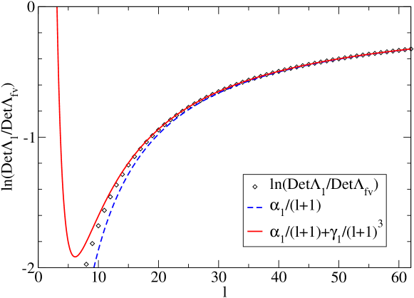
Figure 5: $\ln\left[\mbox{Det}\Lambda^{(l)}/\mbox{Det}\Lambda^{(l)}_{\rm free}\right]$ for the single bounce, for parameter values: $\beta=45$, $b=0.25$, $\epsilon=0.046$, $\varphi(0)=\varphi_{\rm tv}-0.000\,551\,736\,739\,278\,415\,5$, $\varphi(\pi)=\varphi_{\rm fv}+0.000\,001\,929\,113\,943\,772\,119\,407\,698\,5$. Diamond points denote the numerical results using the Gel’fand-Yaglom technique as in (4.29)-(4.30); the (blue) dash line denotes the leading large $l$ behavior in (4.31) with $\alpha$ defined in (4.33) and $\gamma=0$; the (red) solid line denotes the leading and subleading large $l$ behavior in (4.31) with $\alpha$ in (4.33) and $\gamma$ defined in (4.34).

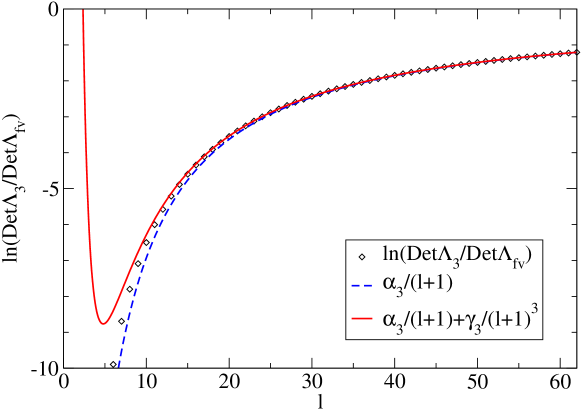
Figure 6: $\ln\left[\mbox{Det}\Lambda^{(l)}/\mbox{Det}\Lambda^{(l)}_{\rm free}\right]$ for the triple bounce, for parameter values: $\beta=45$, $b=0.25$, $\epsilon=0.046$, $\varphi(0)=\varphi_{\rm tv}-0.007\,517\,937\,804\,678\,529$, $\varphi(\pi)=\varphi_{\rm fv}+0.001\,906\,935\,294\,979\,618$. Diamond points denote the numerical results using the Gel’fand-Yaglom technique as in (4.29)-(4.30); the (blue) dash line denotes the leading large $l$ behavior in (4.31) with $\alpha$ defined in (4.33) and $\gamma=0$; the (red) solid line denotes the leading and subleading large $l$ behavior in (4.31) with $\alpha$ in (4.33) and $\gamma$ defined in (4.34).

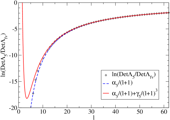
Figure 7: $\ln\left[\mbox{Det}\Lambda^{(l)}/\mbox{Det}\Lambda^{(l)}_{\rm free}\right]$ for the quintuple bounce, for parameter values: $\beta=45$, $b=0.25$, $\epsilon=0.046$, $\varphi(0)=\varphi_{\rm tv}-0.303\,787\,546\,677\,413\,1$, $\varphi(\pi)=\varphi_{\rm fv}+0.187\,525\,348\,746\,153\,5$. Diamond points denote the numerical results using the Gel’fand-Yaglom technique as in (4.29)-(4.30); the (blue) dash line denotes the leading large $l$ behavior in (4.31) with $\alpha$ defined in (4.33) and $\gamma=0$; the (red) solid line denotes the leading and subleading large $l$ behavior in (4.31) with $\alpha$ in (4.33) and $\gamma$ defined in (4.34).

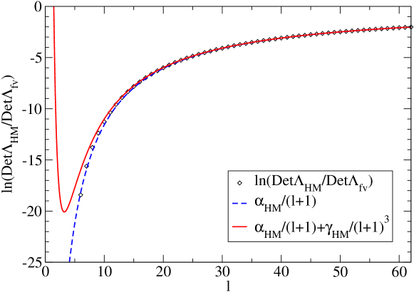
Figure 8: $\ln\left[\mbox{Det}\Lambda^{(l)}/\mbox{Det}\Lambda^{(l)}_{\rm free}\right]$ for the Hawking-Moss bounce, for parameter values: $\beta=45$, $b=0.25$, $\epsilon=0.046$. Diamond points denote the numerical result using the Gel’fand-Yaglom technique as in (4.29)-(4.30); the (blue) dash line denotes the leading large $l$ behavior in (4.31) with $\alpha$ defined in (4.33) and $\gamma=0$; the (red) solid line denotes the leading and subleading large $l$ behavior in (4.31) with $\alpha$ in (4.33) and $\gamma$ defined in (4.34).

We have computed these determinants as a function of $l$, by numerically integrating the initial value problem (4.29) for various bounce solutions, using the fluctuation equation in (3.18), with metric field given by the de Sitter form (4.24), and the scalar field given by solutions to the bounce equation (4.25). The scalar field bounce solutions in this de Sitter case with same parameter $\beta=45$ are very close to those shown in Figures 2, 3 and 4, so we do not bother plotting them again. The results for the logarithm of the determinant ratio are shown as diamond points in Figures 5 through 8. The first empirical observation is that the large $l$ behavior is very similar to that (4.22) found in the flat space case dunnemin :

$$\ln\left[\frac{\mbox{Det}(\Lambda^{(l)})}{\mbox{Det}(\Lambda_{\rm free}^{(l)})}\right]\sim\frac{\alpha}{l+1}+\frac{\gamma}{(l+1)^{3}}+\dots\quad,\qquad l\to\infty\quad,$$ (4.31)

To extract the leading coefficient $\alpha$, we consider the leading and subleading large $l$ behavior of the Jacobi equation (3.18):

$$-\ddot{\Phi}^{(l)}-3\frac{\dot{a}}{a}\dot{\Phi}^{(l)}+\left[V^{\prime\prime}(\phi)+2\kappa\dot{\phi}^{2}+\frac{l(l+2)}{a^{2}}\right]\Phi^{(l)}=\lambda^{(l)}\Phi^{(l)}\quad,\qquad(l\gg 1)\quad.$$ (4.32)

Adapting the WKB analysis of dhlm ; dunnemin leads to the following result for the leading large $l$ dependence of the log of the determinant ratio:

$$\alpha=\frac{1}{2}\int_{0}^{\sigma_{\rm max}}d\sigma\,a(\sigma)\left[V^{\prime\prime}(\phi)+2\kappa\dot{\phi}^{2}-V^{\prime\prime}(\phi_{\rm fv})\right]\quad,$$ (4.33)

Notice the close similarity to the leading term in the flat space large $l$ behavior in (4.22). This curved-space leading behavior $\alpha/(l+1)$, with $\alpha$ given by (4.33), is shown in Figures 5 through 8 as dashed (blue) curves, and we see that the agreement at large $l$ is very good. It is much harder to find the next-to-leading behavior because the subleading $l$ dependence of the Jacobi equation is very complicated. Nevertheless, by analogy with the flat space case (4.22) we propose the estimate

$$\gamma\approx-\frac{1}{8}\int_{0}^{\sigma_{\rm max}}d\sigma\,a^{3}(\sigma)\left[V^{\prime\prime}(\phi)+2\kappa\dot{\phi}^{2}-V^{\prime\prime}(\phi_{\rm fv})\right]\left[V^{\prime\prime}(\phi)+2\kappa\dot{\phi}^{2}+V^{\prime\prime}(\phi_{\rm fv})\right].$$ (4.34)

Including this subleading behavior in (4.31) produces the solid (red) curves in Figures 5 through 8, and we see that the agreement with the exact numerical results is noticeably improved and is excellent at large $l$, and is characteristic of an asymptotic large $l$ expansion in its behavior at small $l$. Thus, the estimate in (4.34) is very close to the exact answer. We found similar behavior for other bounces.

V Negative modes

In this section we turn to another important property of the fluctuation operator, namely the existence of negative modes. Here, to be more general we can return to the general bounce solutions, not needing to work in the de Sitter limit any more (although we find the results to be the same in either case). In the flat space false vacuum decay problem, it has been shown that the fluctuation problem (3.19) has one and only one negative mode, and that this occurs in the $l=0$ sector coleman3 . This single negative mode plays an important physical role in the semiclassical quantization, accounting for the decaying nature of the process langer ; stone ; coleman1 . In the gravitational case, there has been considerable effort analyzing the appearance of negative modes in the $l=0$ sector tanaka ; turok1 ; turok2 ; lav1 ; lav2 ; lav3 . For the scalar field fluctuations characterized by the secondary action (3.14), the oscillating $n$-bounce solution has $n$ negative modes in the $l=0$ sector lav3 . Here we show that the higher $n$ oscillating bounce solutions also can have negative modes in higher $l$ sectors, while the single bounce solution, the Coleman-De Luccia solution, has precisely one negative mode, which is for $l=0$.

A direct numerical method for counting negative modes is based on an important theorem in the calculus of variations due to Morse morse . It states that the number of negative modes of the fluctuation operator $\Lambda$ is given by the number of zeros of the solution of the initial value Jacobi equation $\Lambda\Phi=0$. This is consistent with the related Gel’fand-Yaglom result (4.21) for the computing the determinant as the value of $\Phi(\sigma_{\rm max})$, since an odd number of zeros leads to a negative determinant. This Morse analysis has been applied to the counting of negative modes in the flat space false vacuum decay problem in maziashvili .

Table 1: The number of negative modes without including the degeneracy factor $(l+1)^{2}$, for the parameter values: $\beta=45$, $\epsilon=0.23$.

$l$	0	2	3	4	5	6	7
1-bounce	1	0	0	0	0	0	0
3-bounce	3	2	2	1	1	0	0
5-bounce	5	4	3	2	1	0	0
HM	6	4	3	2	1	0	0

So to count the number of negative modes for a given bounce solution, we numerically integrate the fluctuation Jacobi equation (3.18), with initial value boundary condition $\Phi^{(l)}\sim\sigma^{l}$, and count how many times this function changes sign on the interval $[0,\sigma_{\rm max}]$. In this case we can do this computation using the full bounce solutions as obtained in Section II, not just in the de Sitter limit where the metric function $a(\sigma)$ is chosen to take the sinusoidal form (4.24). In this way, we confirm the results of turok2 ; lav3 that the $n$-bounce solution has $n$ negative modes in the $l=0$ sector. More surprisingly, we find that for $l\geq 2$ there are some negative modes for the higher $n$ oscillating bounce solutions. The precise pattern depends on the parameters in the potential, but a representative counting is shown in Table 1. As the oscillation number of the bounce increases there are more negative modes, and they extend to higher values of $l$. In studying many single-bounce solutions we have always found only one negative mode, and always in the $l=0$ sector. We also found the same negative mode counting pattern using Lavrelashvili et al’s fluctuation operator in (A.2).

To put this result of extra negative modes at higher $l$ in some perspective, consider the Hawking-Moss solution, which is the large $n$ limit of the $n$-bounce solution hw . Here, we can write the exact solution to the zero eigenvalue Jacobi equation, $\Lambda\Phi=0$, with initial behavior $\Phi\sim\sigma^{l}$, as an associated Legendre function, analogous to the false vacuum solution in (4.27):

$$\Phi_{\rm HM}^{(l)}(\sigma)=\frac{N_{\rm HM}}{\sin\left(H_{\rm top}\sigma\right)}P^{l+1}_{-\frac{1}{2}+\sqrt{\beta+\frac{9}{4}}}\left[\cos\left(H_{\rm top}\sigma\right)\right]\quad.$$ (5.35)

Here $\beta$ is the parameter defined in (2.10), and $N_{\rm HM}$ is an unimportant normalization constant. The counting of the zeros of this function can be done precisely, and one finds that the number of zeros depends critically on the value of $\beta$. For $N(N+3)<\beta\leq(N+1)(N+4)$, there are $N+1$ zeros. By the Morse theorem the number of nodes of this zero mode solution is equal to the number of negative modes in the perturbation. This counting is also shown as the last row in Table 1, and we have also confirmed that the numerical integration and the exact result give the same counting. Since the oscillating bounce solutions tend to this Hawking-Moss solution, this goes some way towards explaining the origin of these new negative modes for the oscillating bounce solutions at higher $l$. Physically, this is extra evidence that these higher $n$ oscillating bounce solutions are not directly related to quantum tunneling, as suggested already in hw .

VI Conclusion

In this paper we have analyzed several issues concerning the quantum fluctuations about classical bounce solutions in the theory of a self-interacting scalar field interacting with gravity. In flat space the semiclassical fluctuation analysis can be done completely, both analytically in the thin-wall limit and numerically for more general potentials. In the gravitational case, the fluctuation problem still separates into a set of one-dimensional fluctuation problems labeled by an integer $l$. We found the leading large $l$ behavior (4.31) - (4.33), and an estimate (4.34) for the subleading behavior, of the logarithm of the determinant of the fluctuation operator. The agreement with the numerical computations is impressive. We also analyzed the existence of negative modes using Morse’s theorem, confirming that the single-bounce Coleman-De Luccia solution has a single negative mode, which lies in the $l=0$ sector, and that the oscillating $n$-bounce solution has $n$ negative modes in the $l=0$ sector. We also found new negative modes for the oscillating $n$-bounce solutions for higher $n$ with $l\geq 2$. This adds further weight to the physical interpretation suggested in hw that these bounces are not directly related to quantum tunneling, but rather are related to the thermal character of quantum field theory in de Sitter space, and interpolate to the Hawking-Moss solution for large $n$.

Many problems remain. The standard scalar fluctuation analysis turok1 ; turok2 ; lav1 ; lav2 in the gravitational case precludes consideration of the $l=1$ sector, and so we cannot yet say anything about the collective coordinate contribution to the renormalized fluctuation determinant. In the flat space case it was recently shown how this $l=1$ contribution, combining the determinant with the zero modes removed and the collective coordinate contribution, could be expressed simply in terms of the asymptotic properties of the classical bounce solution dunnemin . Whether something like this can be found for the gravitational case depends on a different analysis of the $l=1$ fluctuation problem. Perhaps the most challenging problem is that the renormalization of quantum gravity is not understood. In the flat space case, without gravity, the subtractions made from the regularized determinant for each $l$ include a finite piece depending on the regularization scale. These can be associated with renormalization, permitting the computation of a finite and renormalized fluctuation determinant baacke ; dunnemin . An important preliminary step for the gravitational case would be to develop fully this approach in the limit where the gravitational background is fixed to be de Sitter, in which case the large $l$ behavior of the log determinants is given by (4.31), and where the perturbative renormalization of the scalar field in a fixed curved background is known birrell . Hopefully this can shed further light on the important question of the nature of the semiclassical path integral approximation in the presence of de Sitter gravity rubakov ; garriga ; vachaspati .

Acknowledgments: We thank the US DOE for support through the grant DE-FG02-92ER40716.

Appendix A Related forms of the fluctuation operator

In discussing the existence of negative modes it is possible to make other choices than (3.17) for the weight function, yielding superficially different-looking Jacobi equations turok1 ; turok2 ; lav1 ; lav2 ; lav3 . But for the purposes of computing the determinant, where the magnitude of the eigenvalues is also relevant, the choice in (3.18) is the most direct. For completeness, the choice of Lavrelashvili et al is to use the perturbation function $\Phi_{L}\equiv\sqrt{a^{3}/{\mathcal{Q}}}\delta\phi$, and weight function $a^{3}/{\mathcal{Q}}$, leading to the Jacobi equation lav1 ; lav2 ; lav3

$$-\frac{d^{2}\Phi_{L}}{d\sigma^{2}}+U_{L}[a,\phi]\Phi_{L}=\lambda_{L}\Phi_{L}\quad,$$ (A.1)

where

$$U_{L}[a,\phi] \equiv \frac{1}{{\mathcal{Q}}}V^{\prime\prime}(\phi)-\frac{3\kappa a^{2}}{2{\mathcal{Q}}^{2}(-\Delta_{3}-3K)}\left[V^{\prime}(\phi)\right]^{2}+\frac{6\kappa a\dot{a}\dot{\phi}}{{\mathcal{Q}}^{2}(-\Delta_{3}-3K)}V^{\prime}(\phi)-\frac{\kappa}{6}\left[\dot{\phi}^{2}+V(\phi)\right]$$ (A.2)

$$+\frac{\dot{a}^{2}}{a^{2}}\left(-\frac{1}{4}-\frac{10}{{\mathcal{Q}}}+\frac{12}{{\mathcal{Q}}^{2}}\right)+\frac{1}{a^{2}}\left[(-\Delta_{3}-3K)({\mathcal{Q}}+2)-\frac{-2\Delta_{3}-8K}{{\mathcal{Q}}}\right]\quad,$$

which agrees with Eqn. (19) in the second reference in lav3 when $K=1$ and $\Delta_{3}=0$. Furthermore, this potential satisfies

$$U_{L}[a,\phi]={\mathcal{Q}}\,U[a,\phi]+\sqrt{\frac{{\mathcal{Q}}}{a^{3}}}\frac{d^{2}}{d\sigma^{2}}\sqrt{\frac{a^{3}}{{\mathcal{Q}}}}\quad.$$ (A.3)

Using this fluctuation operator, we found the same pattern of negative modes shown in Table 1.

Another choice, yielding an elegant result for the existence of negative modes, was made by Turok et al, who chose the perturbation function $\Phi_{T}\equiv\delta\phi/\dot{\phi}$, and weight function $1/\dot{\phi}^{2}$, leading to the Jacobi equation turok1 ; turok2

$$-\frac{d}{d\sigma}\left(\frac{a^{3}\dot{\phi}^{2}}{{\mathcal{Q}}}\frac{d\Phi_{T}}{d\sigma}\right)+U_{T}[a,\phi]\Phi_{T}=\lambda_{T}\Phi_{T}\quad,$$ (A.4)

Here

$$U_{T}[a,\phi]\equiv a\,\dot{\phi}^{2}(-\Delta_{3}-3K)\quad,$$ (A.5)

and it is related to our $U[a,\phi]$ by

$$U_{T}[a,\phi]=a^{3}\dot{\phi}^{2}U[a,\phi]-\dot{\phi}\frac{d}{d\sigma}\left(\frac{a^{2}\ddot{\phi}}{{\mathcal{Q}}}\right)\quad.$$ (A.6)

References

- (1) S. R. Coleman and F. De Luccia, “Gravitational Effects On And Of Vacuum Decay,” Phys. Rev. D 21, 3305 (1980).
- (2) T. Banks, “Heretics of the false vacuum: Gravitational effects on and of vacuum decay. II,” arXiv:hep-th/0211160.
- (3) S. Kachru, R. Kallosh, A. Linde and S. P. Trivedi, “De Sitter vacua in string theory,” Phys. Rev. D 68, 046005 (2003) [arXiv:hep-th/0301240].
- (4) R. Bousso, “Cosmology and the S-matrix,” Phys. Rev. D 71, 064024 (2005) [arXiv:hep-th/0412197].
- (5) A. D. Linde, “Particle Physics and Inflationary Cosmology,” Contemp. Concepts Phys. 5, 1 (2005) [arXiv:hep-th/0503203].
- (6) S. W. Hawking and I. G. Moss, “Supercooled Phase Transitions In The Very Early Universe,” Phys. Lett. B 110, 35 (1982).
- (7) S. J. Parke, “Gravity and the decay of the false vacuum,” Phys. Lett. B 121, 313 (1983).
- (8) E. Mottola and A. Lapedes, “The Inflationary Universe With Gravity,” Phys. Rev. D 27, 2285 (1983); “Existence Of Finite Action Solutions To The Coleman-De Luccia Equations,” Phys. Rev. D 29, 773 (1984).
- (9) L. G. Jensen and P. J. Steinhardt, “Bubble Nucleation And The Coleman-Weinberg Model,” Nucl. Phys. B 237, 176 (1984), “Bubble Nucleation For Flat Potential Barriers,” Nucl. Phys. B 317, 693 (1989).
- (10) K. M. Lee and E. J. Weinberg, “Decay Of The True Vacuum In Curved Space-Time,” Phys. Rev. D 36, 1088 (1987).
- (11) D. A. Samuel and W. A. Hiscock, “Effect of gravity on false vacuum decay rates for O(4) symmetric bubble nucleation,” Phys. Rev. D 44, 3052 (1991).
- (12) V. Balek and M. Demetrian, “A criterion for bubble formation in de Sitter universe,” Phys. Rev. D 69, 063518 (2004) [arXiv:gr-qc/0311040], “Euclidean action for vacuum decay in a de Sitter universe,” Phys. Rev. D 71, 023512 (2005) [arXiv:gr-qc/0409001]; M. Demetrian, “False vacuum decay with gravity in a critical case,” arXiv:gr-qc/0504133.
- (13) J. C. Hackworth and E. J. Weinberg, “Oscillating bounce solutions and vacuum tunneling in de Sitter spacetime,” Phys. Rev. D 71, 044014 (2005) [arXiv:hep-th/0410142]; E. J. Weinberg, “New bounce solutions and vacuum tunneling in de Sitter spacetime,” AIP Conf. Proc. 805, 259 (2006) [arXiv:hep-th/0512332].
- (14) R. Bousso and B. Freivogel, “Asymptotic states of the bounce geometry,” Phys. Rev. D 73, 083507 (2006) [arXiv:hep-th/0511084]; R. Bousso, B. Freivogel and M. Lippert, “Probabilities in the landscape: The decay of nearly flat space,” arXiv:hep-th/0603105.
- (15) T. Banks and M. Johnson, “Regulating eternal inflation,” arXiv:hep-th/0512141; A. Aguirre, T. Banks and M. Johnson, “Regulating eternal inflation. II: The great divide,” arXiv:hep-th/0603107.
- (16) J. S. Langer, “Theory Of The Condensation Point,” Annals Phys. 41, 108 (1967) [Annals Phys. 281, 941 (2000)].
- (17) I. Y. Kobzarev, L. B. Okun and M. B. Voloshin, “Bubbles In Metastable Vacuum,” Sov. J. Nucl. Phys. 20, 644 (1975) [Yad. Fiz. 20, 1229 (1974)]; M. B. Voloshin, “Decay Of False Vacuum In (1+1)-Dimensions,” Yad. Fiz. 42, 1017 (1985) [Sov. J. Nucl. Phys. 42, 644 (1985)].
- (18) M. Stone, “Semiclassical Methods For Unstable States,” Phys. Lett. B 67, 186 (1977).
- (19) S. R. Coleman, “The Fate Of The False Vacuum. 1. Semiclassical Theory,” Phys. Rev. D 15, 2929 (1977) [Erratum-ibid. D 16, 1248 (1977)]; C. G. . Callan and S. R. Coleman, “The Fate Of The False Vacuum. 2. First Quantum Corrections,” Phys. Rev. D 16, 1762 (1977).
- (20) A. Gorsky and M. B. Voloshin, “Particle decay in false vacuum,” Phys. Rev. D 73, 025015 (2006) [arXiv:hep-th/0511095].
- (21) R. V. Konoplich and S. G. Rubin, “Decay Probability For Metastable Vacuum In Scalar Theory,” Yad. Fiz. 42, 1282 (1985); “Decay of the metastable vacuum”, Yad. Fiz. 44, 558 (1986) [Sov. J. Nucl. Phys. 44, 359 (1987)].
- (22) G. Isidori, G. Ridolfi and A. Strumia, “On the metastability of the standard model vacuum,” Nucl. Phys. B 609, 387 (2001) [arXiv:hep-ph/0104016]; A. Strumia, N. Tetradis and C. Wetterich, “The region of validity of homogeneous nucleation theory,” Phys. Lett. B 467, 279 (1999) [arXiv:hep-ph/9808263].
- (23) J. Baacke and G. Lavrelashvili, “One-loop corrections to the metastable vacuum decay,” Phys. Rev. D 69, 025009 (2004) [arXiv:hep-th/0307202].
- (24) G. V. Dunne and H. Min, “Beyond the thin-wall approximation: Precise numerical computation of prefactors in false vacuum decay,” Phys. Rev. D 72, 125004 (2005) [arXiv:hep-th/0511156].
- (25) S. R. Coleman, V. Glaser and A. Martin, “Action Minima Among Solutions To A Class Of Euclidean Scalar Field Equations,” Commun. Math. Phys. 58, 211 (1978).
- (26) S. Gratton and N. Turok, “Cosmological perturbations from the no boundary Euclidean path integral,” Phys. Rev. D 60, 123507 (1999) [arXiv:astro-ph/9902265].
- (27) S. Gratton and N. Turok, “Homogeneous modes of cosmological instantons,” Phys. Rev. D 63, 123514 (2001) [arXiv:hep-th/0008235].
- (28) G. V. Lavrelashvili, “On the quadratic action of the Hawking-Turok instanton,” Phys. Rev. D 58, 063505 (1998) [arXiv:gr-qc/9804056];
- (29) A. Khvedelidze, G. V. Lavrelashvili and T. Tanaka, “On cosmological perturbations in closed FRW model with scalar field and false vacuum decay,” Phys. Rev. D 62, 083501 (2000) [arXiv:gr-qc/0001041].
- (30) T. Tanaka and M. Sasaki, “False vacuum decay with gravity: Negative mode problem,” Prog. Theor. Phys. 88, 503 (1992); T. Tanaka and M. Sasaki, “No supercritical supercurvature mode conjecture in one-bubble open inflation,” Phys. Rev. D 59, 023506 (1999) [arXiv:gr-qc/9808018]; T. Tanaka, “The no-negative mode theorem in false vacuum decay with gravity,” Nucl. Phys. B 556, 373 (1999) [arXiv:gr-qc/9901082].
- (31) G. Lavrelashvili, “Negative mode problem in false vacuum decay with gravity,” Nucl. Phys. Proc. Suppl. 88, 75 (2000) [arXiv:gr-qc/0004025], “The number of negative modes of the oscillating bounces,” Phys. Rev. D 73, 083513 (2006) [arXiv:gr-qc/0602039].
- (32) M. Morse, The Calculus of Variations in the Large, (AMS Colloquium Series Vol. XVIII, 1934).
- (33) I. M. Gel’fand and A. M. Yaglom, “Integration In Functional Spaces And It Applications In Quantum Physics,” J. Math. Phys. 1, 48 (1960).
- (34) S. Levit and U. Smilansky, “A theorem on infinite products of eigenvalues of Sturm-Liouville type operators”, Proc. Am. Math. Soc. 65, 299 (1977).
- (35) R. Forman, “ Functional determinants and geometry ”, Invent. Math. 88, 447 (1987); Erratum, ibid 108, 453 (1992).
- (36) K. Kirsten, Spectral Functions in Mathematics and Physics (Chapman-Hall, Boca Raton, 2002); K. Kirsten and A. J. McKane, “Functional determinants by contour integration methods,” Annals Phys. 308, 502 (2003) [arXiv:math-ph/0305010]; “Functional determinants for general Sturm-Liouville problems,” J. Phys. A 37, 4649 (2004) [arXiv:math-ph/0403050].
- (37) H. Kleinert, Path Integrals in Quantum Mechanics, Statistics, Polymer Physics, and Financial Markets, (World Scientific, Singapore, 2004).
- (38) G. V. Dunne, J. Hur, C. Lee and H. Min, “Calculation of QCD instanton determinant with arbitrary mass,” Phys. Rev. D 71, 085019 (2005) [arXiv:hep-th/0502087].
- (39) Y. Burnier and M. Shaposhnikov, “One-loop fermionic corrections to the instanton transition in two dimensional chiral Higgs model,” Phys. Rev. D 72, 065011 (2005) [arXiv:hep-ph/0507130].
- (40) N. D. Birrell and P. C. W. Davies, Quantum Fields In Curved Space, (Cambridge Univ. Press, 1982).
- (41) V. A. Rubakov and S. M. Sibiryakov, “False vacuum decay in the de Sitter space-time,” Theor. Math. Phys. 120, 1194 (1999) [Teor. Mat. Fiz. 120, 451 (1999)] [arXiv:gr-qc/9905093].
- (42) S. R. Coleman, “Quantum Tunneling And Negative Eigenvalues,” Nucl. Phys. B 298, 178 (1988).
- (43) M. Maziashvili, “Uniqueness of a negative mode about a bounce solution,” J. Phys. A 36, L463 (2003) [arXiv:hep-th/0212283].
- (44) J. Garriga and A. Megevand, “Decay of de Sitter vacua by thermal activation,” Int. J. Theor. Phys. 43, 883 (2004) [arXiv:hep-th/0404097].
- (45) T. Vachaspati and A. Vilenkin, “On The Uniqueness Of The Tunneling Wave Function Of The Universe,” Phys. Rev. D 37, 898 (1988); “Quantum state of a nucleating bubble,” Phys. Rev. D 43, 3846 (1991).