Chiral symmetry restoration at finite temperature in the planar limit.

Abstract:

We investigate numerically chiral symmetry restoration at finite temperature in the planar limit in the deconfined phase, both when it is stable and when the system is supercooled. We find chiral symmetry restoration at $T_{\chi}=T_{d}$, where $T_{d}$ is the temperature of the deconfinement transition in pure gauge theory and $T_{\chi}<T_{d}$ in the supercooled deconfined phase. In the stable case the spectrum of the Dirac operator opens a gap in a discontinuous manner and in the supercooled phase the gap seems to vanish continuously.

1 Introduction.

At finite temperature QCD undergoes qualitative changes of great physical interest. Although much is known, the complicated strongly coupled aspects of the transition region are not under full theoretical control.

At a large number of colors, in the ’t Hooft limit, the system simplifies somewhat [1]. The major effects occur now in the pure gauge sector, while the fermions only react to these effects, without influencing them by back reaction (except, as explained later, by aligning the pure gauge vacuum). The purpose of this paper is to present numerical results on chiral symmetry restoration at finite temperature in the planar limit. Our study is at zero quark mass. Preliminary results have been presented last year [2].

At infinite $N_{c}$ the free energy is temperature ($T$) independent at order $N_{c}^{2}$ for $T<T_{d}$, where $T_{d}$ is the deconfinement temperature. Chiral symmetry is spontaneously broken and the condensate $\frac{1}{N_{c}}\langle\bar{\psi}\psi\rangle$ is nonzero and temperature independent [3, 4]. The chiral symmetry breakdown is reflected by a condensation of eigenvalues of the Euclidean Dirac operator near zero. This condensation emerges naturally in a random matrix context. Because of the infinite number of colors and the lack of relevance of the size of the system due to large $N_{c}$ reduction, one can think of the Euclidean Dirac operator ($D$) as a large random anti-hermitian matrix, whose structure is restricted only by chiral symmetry.

$$D=\pmatrix{0&C\cr-C^{\dagger}&0}$$ (1)

In the spirit of Wigner’s approach to complex nuclei, one is lead to write down the simplest probability distribution for the matrix $C$ [5], whose linear dimension is proportional to $N_{c}$:

$$P(C)\propto e^{-\kappa\dim(C)TrC^{\dagger}C}$$ (2)

Chiral symmetry breaking is then an immediate result, giving it the appearance of a generic phenomenon.

As the temperature is raised, at $T=T_{d}$, a first order deconfinement transition occurs at all $N_{c}\geq 3$; $T_{d}$ has a finite large $N_{c}$ limit [6, 7]. For high temperatures, $T>>T_{d}$, one expects chiral symmetry to be restored and, consequently, the random matrix viewpoint that worked for $T<T_{d}$ to become invalid. The simplest way in which chiral symmetry can get restored is for the Euclidean Dirac operator to open a gap at zero. One might have thought that this effect can be incorporated into an extended random matrix model [8], but, a numerical investigation to be described later on, indicates that the types of random matrix models one would naturally guess will not work when chiral symmetry is unbroken. For $T<T_{d}$ random matrix theory applies also at finite $N_{c}$, but, without going to the planar limit the argument does not extend to high temperatures  [9], where there is no energy regime dominated by Goldstone particles [10]. We see that going to infinite $N_{c}$ does not help in this respect.

2 Large $N_{c}$ in the deconfined phase.

At $T>T_{d}$, in the deconfined phase, the free energy of the gluons starts depending on $T$. Feynman diagrams containing fermion loops are still suppressed by one power of $\frac{1}{N_{c}}$, so long as the number of flavors is kept fixed, as we do.

In the Euclidean path integral formulation, physical finite temperature is reflected by the “time” direction being compactified to a circle of radius $\frac{1}{T}$ and bosons/fermions having periodic/antiperiodic boundary conditions in the time direction. For $T<T_{c}$ the boundary conditions are irrelevant, since the preservation of the related $Z(N_{c})\to U(1)$ global symmetry washes them out. When $T>T_{d}$, the trace of parallel transport round the temporal circle (Polyakov loop) acquires a fixed phase and breaks spontaneously the associated $Z(N_{c})$. Which phase is picked is arbitrary in the absence of fermions, as all phases have the same gluonic energy. When fermions are present, although in general their contribution to the free energy is subleading, they fix the phase of the Polyakov loop to one specific value because the fermions break the $Z(N_{c})$ explicitly and align the vacuum. It is physically plausible, and supported by our numerical work, that the phase is chosen to make the Polyakov loop positive. This preserves CP, but also making the Polyakov loop negative would have. Other than aligning the vacuum, fermions have no impact on the distribution of the gluonic fields at infinite $N_{c}$.

3 Lattice setup.

We work on a hypercubic lattice of shape $L_{4}L^{3}$. The gauge action is of single plaquette type.

$$S=\frac{\beta}{4N_{c}}\sum_{x,\mu\neq\nu}Tr[U_{\mu,\nu}(x)+U_{\mu,\nu}^{\dagger}(x)]$$ (3)

$$U_{\mu,\nu}(x)=U_{\mu}(x)U_{\nu}(x+\hat{\mu})U_{\mu}^{\dagger}(x+\hat{\nu})U_{\nu}^{\dagger}(x)$$ (4)

We define $b=\frac{\beta}{2N^{2}_{c}}=\frac{1}{g^{2}N_{c}}=\frac{1}{\lambda}$ and take the large $N_{c}$ limit with $b$ held fixed. As usual, $b$ determines the lattice spacing $a$ and $\lambda$ is the ’t Hooft coupling. The gauge fields are periodic. $x$ is a four component integer vector labeling the site, and $\mu$ labels a direction; a unit vector in the $\mu$ direction is denoted by $\hat{\mu}$. The link matrices $U_{\mu}(x)$ are in $SU(N_{c})$.

There is a $Z^{4}(N_{c})$ symmetry under which

$$U_{\mu}(x)\rightarrow e^{\frac{2\pi\imath k_{\mu}}{N_{c}}}U_{\mu}(x)$$ (5)

for all $x$ with $x_{\mu}=c_{\mu}$. The integers $c_{\mu}$ are fixed, and the integers $k_{\mu}$ label the elements of the $\mu$-th $Z(N_{c})$ group; $c_{\mu}=0,1,..,L_{\mu}-1$. Changing the $c_{\mu}$’s amounts to a local gauge transformation. We have $L_{1}=L_{2}=L_{3}=L$.

The Polyakov loop matrix is denoted by $P_{4}(x)$ and defined by:

$$P_{4}(x)=U_{4}(x)U_{4}(x+\hat{4})U_{\mu}(x+2\cdot\hat{4})..U_{\mu}(x+(L_{4}-1)\cdot\hat{4})$$ (6)

Under the $Z(N_{c})$ factor associated with the time direction, $P_{4}(x)$ gets multiplied by a phase. The gauge invariant content of $P_{4}(x)$ is its set of eigenvalues (the spectrum) $e^{\imath\theta^{P}_{i}},~{}i=1,2...,N_{c}$. The ordering is not gauge invariant, and there is a constraint that $\det P_{4}(x)=1$. Under the $Z(N_{c})$ transformation, the set of eigenvalues is circularly shifted by a fixed amount. The spectrum of $P_{4}(x)$ and of $P_{4}(x+j\cdot\hat{4})$ are the same for all $j=0,1,2....,L_{4}-1$.

For a fixed $b$ in a certain range, if $L$ is large enough, the global $Z^{3}(N_{c})$ symmetry associated with the spatial directions is unbroken. In practice, it is even possible to work in metastable phases, as long as these $Z(N_{c})$’s are maintained.

Depending on $L_{4}\leq L$ the $Z(N_{c})$ in the time direction may be broken or not. Alternatively, for $L_{4}\leq L$, one can break the time-$Z(N_{c})$ by increasing $b$ (for $L_{4}=L$, we view as time the one particular, but randomly selected, direction that breaks its $Z(N_{c})$). The breaking point is the deconfinement transition. There is no dependence on $L$ on either side of this transition so long as $b$ is in the range which preserves the spatial $Z^{3}(N_{c})$ [11]; this will always be the case.

In lattice units we have $aT_{d}=\frac{1}{L_{c}(b)}$, where [11]

$$b\rightarrow b_{I}\equiv be(b)~{}~{}~{}~{}~{}~{}~{}e(b)=\frac{1}{N}\langle TrU_{\mu,\nu}(x)\rangle$$ (7)

$$L_{c}(b)~{}\sim 0.260(15)\left(\frac{11}{48\pi^{2}b_{I}}\right)^{\frac{51}{121}}e^{\frac{24\pi^{2}b_{I}}{11}}$$ (8)

In [11] it was found that planar gauge theory on the torus can exist in five phases, $0$c,$1$c,..,$4$c; the deconfined phase is the 1c phase in this notation.

The fermion action is given by the overlap Dirac operator which preserves chiral symmetry exactly. This choice makes it possible to pose the question of spontaneous chiral symmetry breaking in a clean way.

The massless overlap Dirac operator [12], $D_{o}$, is defined by:

$$D_{o}=\frac{1+V}{2}$$

$$V^{-1}=V^{\dagger}=\gamma_{5}V\gamma_{5}={\rm sign}(H_{w}(M))\gamma_{5}$$ (9)

$H_{w}(M)$ is the Wilson Dirac operator at mass $M$, which we shall choose as $M=-1.5$. $M$ should not be confused with a bare quark mass.

$$H_{w}(M)=\gamma_{5}\left[M+4-\sum_{\mu}\left(\frac{1-\gamma_{\mu}}{2}T_{\mu}+\frac{1+\gamma_{\mu}}{2}T_{\mu}^{\dagger}\right)\right]$$ (10)

The $T_{\mu}$ matrices are the lattice generators of parallel transport and depend parametrically and analytically on the lattice links $U_{\mu}(x)$.

The internal fermion-line propagator, $\frac{2}{1+V}$ is not needed at infinite $N_{c}$, since fermion loops are suppressed. For fermion lines continuing external fermion sources we are allowed to use a slightly different quark propagator [13] defined by:

$$\frac{1}{A}=\frac{1-V}{1+V}$$ (11)

$A=-A^{\dagger}$ and anticommutes with $\gamma_{5}$. The spectrum of $A$ is unbounded, but is determined by the spectrum of $V$ which is restricted to the unit circle. Up to a dimensionful unit, $A$ should be thought of as a lattice realization of the continuum massless Dirac operator, $D$:

$$2|M|A\leftrightarrow D=\gamma_{\mu}\partial_{\mu}+.....$$ (12)

Our main observable will be the smallest eigenvalue of the non-negative matrix $-A^{2}$, which is the discrete version of $D^{\dagger}D$, where $D$ is the continuum, Euclidean, Dirac operator in a fixed gauge background. The gauge background varies according to the pure gauge action and we shall look at the induced probability distribution of the smallest eigenvalues of $-A^{2}$.

Let $\lambda_{1,2}$ be the two lowest eigenvalues of $\sqrt{-A^{2}}$: The dimensionless gap as a function of the dimensionless temperature $t$, $g(t)$, is defined as the average over gauge configurations of $\lambda_{1}(b,L,L_{4})L_{c}(b)$. The dimensionless temperature itself is defined as $L_{c}(b)/L_{4}$.

At infinite $N_{c}$, $g$ will vanish when the symmetry is spontaneously broken. If we find that $g$ is nonzero, we know that chiral symmetry is restored. This is true because the single way chiral symmetry transformations can avoid inducing naive relations among correlation functions of physical observables is by the matrix $A^{-1}$ becoming singular with finite probability. If $g>0$ almost surely, this cannot happen and chiral symmetry is preserved.

As we vary $L_{4}$ or $b$, $g$ will change. If the change is discontinuous to or from zero, the transition is of first order; otherwise, it is continuous. We shall find that $g$ jumps discontinuously from zero to a finite value exactly when the pure gauge field undergoes the phase transition. Also, we shall see some evidence that when we lower the temperature $T$ below $T_{d}$, but stay in a supercooled deconfined phase, eventually, $g$ goes to zero at some temperature $T_{\chi}<T_{d}$; this chiral symmetry breaking transition, occurring as the temperature is lowered in the supercooled deconfined phase, seems continuous within our numerical resolution.

4 Vacuum alignment.

We wish first to check that indeed the vacuum of the gauge fields is selected by aligning with the fermions in the manner discussed earlier.

Numerically, we would like to show that the (positive) fermion determinant is indeed favoring a positive Polyakov loop in the deconfined phase. We do this as follows:

We let the lattice system pick an arbitrary phase for its Polyakov loop in the deconfined phase. We now define the fermions with twisted boundary conditions relative to this phase in the time direction. That is, the fermions obey the boundary condition $\psi(0)=-\psi(\frac{1}{T})e^{\imath(\theta-\phi)}$, where the Polyakov loop has phase $e^{\imath\phi}$. We now intend to show that the fermion determinant is maximal when $\theta=0$.

A complete computation of the determinant is too expensive and might be an overkill. We accept the hypothesis that the determinant is maximal when the gap $g$ is. After all, the eigenvalues of the Dirac operator repel and a larger $g$ simply would push all eigenvalues to slightly higher values, hence increasing the determinant itself.

In summary we end up focusing on the gap $g$ as a function of the angle $\theta$. As expected, we obtain a periodic function of $\theta$ with a local maximum at $\theta=0$ and local minima at $\theta=\pm\pi$, symmetric under $\theta\to-\theta$ and monotonically decreasing from its value at $\theta=0$ to its value at $\theta=\pi$.

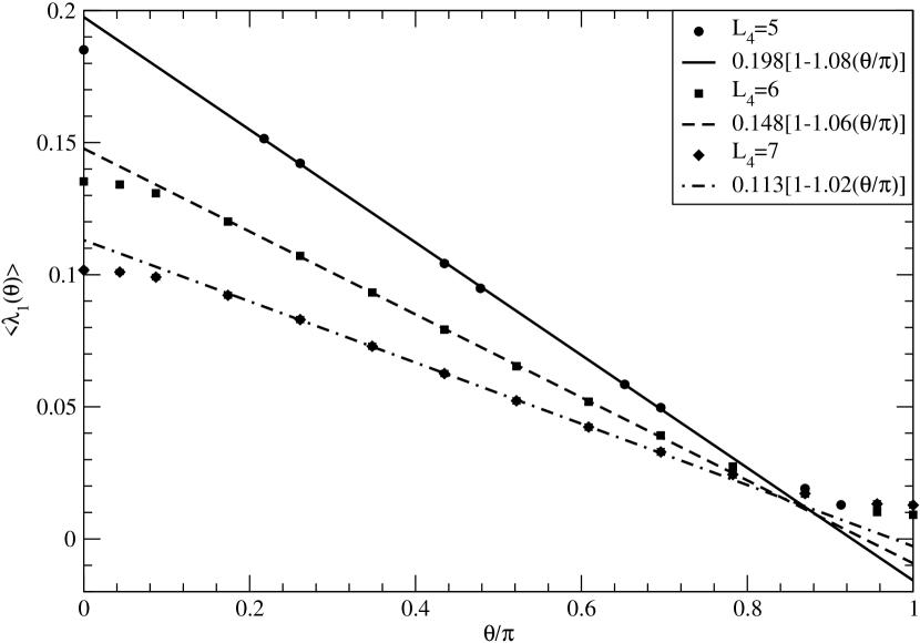
Figure 1: The gap as a function of twist.

CP invariance implies $\frac{dg}{d\theta}=0$ at $\theta=0,\pi$; figure 1 also shows that the region of maximum is connected by an approximately linear segment to the regions of the minima.

This linearity can be understood if one accepts a static approximation, which is plausible for high enough temperatures. In this static approximation the gauge field in the time direction is taken as a constant, and the gauge fields in the space directions are taken as time independent. In the continuum, the spectrum of the operator $\gamma_{4}D$ (where 4 labels the time direction) has its spectrum linearly shifted by $\frac{T\theta}{\pi}$; assuming now that this shift gets transmitted almost intact to the lower bound of the operator $D^{\dagger}D$, we obtain the linearity of the gap $g$ with a predicted slope.

Note however, that as the temperature is lowered towards $T_{d}$, $T$ gets replaced by a smaller temperature, $T_{eff}<T$. Still, the gap is maximal at $\theta=0$ and vanishes at $\theta=\pm\pi$, and the linear portion is always present.

One might have expected to find the gap vanishing before $\theta$ reaches $\pm\pi$, for the following reason: Parallel transport round the time direction results in a unitary matrix whose spectrum has support on a connected arc on the unit circle, centered at unity. Because of the finite width, one could have imagined that in some color direction fermions are effectively defined with a twisted boundary condition and the static approximation would have predicted an earlier point where the gap associated with that color direction vanishes. We do not see this happening, indicating that there is no sense in which the eigenvalues associated with the Polyakov loop can be used to coherently select special orientations in color space for the fermions. All that one can expect is an incoherent effect, in which the spread in eigenvalues influences averages over all colors – a point we shall return to later.

In [8] the static approximation was used to motivate a variation on the random matrix model describing the Dirac operator in the confined phase. The Dirac operator is now split into blocks labeled by the Matsubara integer $n$, and each block has a structure

$$D_{n}=\pmatrix{0&C+\imath[(2n+1)\pi-\theta]T\cr-C^{\dagger}+\imath[(2n+1)\pi-\theta]T&0}$$ (13)

with a common matrix $C$ distributed according to equation 2.

In this picture the Polyakov loop is taken as a unit matrix with one overall phase. If we generalized the above random model by further splitting into blocks associated with each color we would obtain a prediction that the $g(\theta)$ ought to vanish before $\theta$ reaches $\pm\pi$, but this is somewhat implausible and indeed does no happen as pointed out above.

5 A possible implication of the spread in the eigenvalues associated with the Polyakov loop.

We present here a suggestion that the spread in eigenvalues explains why one obtains an effective temperature $T_{eff}<T$ when one gets closer to $T_{d}$ from above.

Consider a free Dirac fermion in continuum with twisted boundary condition $\theta$. Let $f$ be the contribution of this one fermion to the free energy density in Euclidean space. Standard manipulations [14] produce

$$f=4\left[-\frac{\pi^{4}}{90}+\frac{\left(1-(\frac{\theta}{\pi})^{2}\right)^{2}}{48}\right]T^{4}$$ (14)

For $\theta=0$ we recover the well known expression. As $\theta$ increases toward $\pi$ the coefficient of $T^{4}$ decreases and eventually even changes sign. Indeed, at $\theta=\pi$ we have boundary conditions appropriate for a boson, but since we kept the determinant at a positive power, we used for it Fermi statistics. Had we used the right statistics, the determinant would have been at a negative power and then the contribution to $f$ would have had the normal sign.

We now speculate that the fact that parallel transport round the compact direction is best described with a phase drawn from a distribution symmetric about zero but not of zero width, effectively implies an averaging over $\theta$ in the above equation. In turn, this could be viewed as an effective reduction of the temperature, if one insists on keeping the classical value for the prefactor.

For large $T$, $T>>T_{d}$, the width of the distribution shrinks to zero and the effect goes away. However, for $T$ close enough to $T_{d}$, this indicates that $f\approx c(T)T^{4}$ where $c(T)$ decreases from its classical value at $T=\infty$ slowly. The fermionic contribution to the free energy would therefore appear almost noninteracting, however with a coefficient that is slightly off.

Much more is needed to see if this speculation bears out.

6 Supercooling.

So long as we have confinement we ought to have spontaneous symmetry breakdown at infinite $N_{c}$ for theoretical reasons [15]. We also know from numerical work that the deconfinement transition in planar QCD is of first order.

We now ask what happens to chiral symmetry as we supercool the deconfined phase, to temperatures $T<T_{d}$. The gauge coupling should increase, and eventually, chiral symmetry could break again, this time without confinement. We address this question numerically. Because of the need to extrapolate into the metastable phase, the conclusion is quite tentative.

We see an indication that there is a chiral symmetry breaking temperature $T_{\chi}<T_{d}$, where chiral symmetry is broken in the supercooled deconfined phase. Our numerical finding is consistent with a continuous transition at $T_{\chi}$.

Our numerical results are collected in table 1. All the results are in the $1$c phase and we have used anti-periodic boundary conditions for fermions with respect to the Polyakov loop in the broken direction. We studied five different couplings, namely, $b=0.35$, $b=0.3525$, $b=0.355$, $b=0.3575$ and $b=0.36$. We will use the following central value for the critical sizes at these couplings:

$$L_{c}(0.35)=5.97; \ \ \ L_{c}(0.3525)=6.46;\ \ \ L_{c}(0.355)=6.96;$$ (15)

$$L_{c}(0.3575)=7.47; \ \ \ L_{c}(0.36)=8.01.$$ (16)

We performed a careful study at $b=0.3525$ and $L_{4}=L=6$ and convinced ourselves that the large $N$ limit is obtained for values listed in the table. With the exception of the entry at $b=0.355$, $N=23$, $L=8$ and $L_{4}=7$, all entries are definitely in the stable $1$c phase. It is possible that the $b=0.355$, $N=23$, $L=8$ and $L_{4}=7$ entry is in the supercooled $1$c phase.

Table 1: Results for the lowest two eigenvalues and their correlation $c$ as defined in (18) are listed for several values of $b$, $L$, $L_{4}$ and $N$ in the $1$c phase.

$b$	$N$	$L$	$L_{4}$	$\langle\lambda_{1}\rangle$	$\langle\lambda_{2}\rangle$	$c$
0.3500	43	6	2	0.7752(5)	0.7780(5)	0.94(2)
0.3500	43	6	3	0.4199(7)	0.4249(6)	0.93(3)
0.3500	43	6	4	0.2565(7)	0.2648(6)	0.68(8)
0.3500	43	6	5	0.1591(10)	0.1693(8)	0.73(8)
0.3525	43	6	2	0.7728(5)	0.7753(5)	0.95(2)
0.3525	43	6	3	0.4189(6)	0.4233(6)	0.94(3)
0.3525	43	6	4	0.2602(6)	0.2671(5)	0.79(5)
0.3525	43	6	5	0.1674(11)	0.1771(10)	0.85(5)
0.3525	31	6	6	0.1130(14)	0.1277(12)	0.71(7)
0.3525	31	6	6	0.1069(21)	0.1219(18)	0.87(7)
0.3525	37	6	6	0.1038(19)	0.1168(17)	0.89(3)
0.3525	43	6	6	0.1091(15)	0.1223(10)	0.73(12)
0.3525	43	6	6	0.1049(16)	0.1179(12)	0.89(3)
0.3525	47	6	6	0.1016(13)	0.1136(12)	0.82(4)
0.3525	47	6	6	0.1030(13)	0.1162(12)	0.75(8)
0.3525	53	6	6	0.1023(13)	0.1136(10)	0.81(6)
0.3525	53	6	6	0.0992(14)	0.1116(12)	0.87(3)
0.3550	43	6	6	0.1189(12)	0.1314(11)	0.82(8)
0.3550	23	8	7	0.0623(17)	0.0767(13)	0.79(7)
0.3575	43	6	6	0.1327(12)	0.1417(12)	0.89(3)
0.3575	43	6	6	0.1325(11)	0.1423(10)	0.89(3)
0.3575	23	8	7	0.0868(13)	0.0975(11)	0.86(5)
0.3600	37	6	2	0.7610(6)	0.7636(5)	0.97(1)
0.3600	37	6	3	0.4141(6)	0.4196(4)	0.82(5)
0.3600	37	6	4	0.2654(8)	0.2725(7)	0.79(7)
0.3600	37	6	5	0.1849(9)	0.1929(8)	0.87(4)
0.3600	37	7	5	0.1832(6)	0.1891(5)	0.80(5)
0.3600	37	7	5	0.1823(7)	0.1891(4)	0.76(8)
0.3600	23	8	5	0.1837(7)	0.1904(6)	0.82(5)
0.3600	23	8	6	0.1310(9)	0.1395(7)	0.75(6)
0.3600	23	8	7	0.0963(10)	0.1064(8)	0.80(11)
0.3600	37	8	5	0.1807(5)	0.1861(4)	0.80(6)
0.3600	37	6	6	0.1329(13)	0.1430(12)	0.91(3)
0.3600	43	6	6	0.1353(10)	0.1445(9)	0.83(6)

The data at the largest $N$ from table 1 was used to obtain the dimensionless gap, $g(t)$, as a function of the dimensionless temperature $t$. Figure 2 shows all the data for $t<2.8$. There is some spread of points, indicative of order $a^{2}$ lattice corrections, but the data seems to condense toward a line to which we assign a physical meaning in the continuum. We show a two parameter fit to

$$g=1.76\sqrt{t-0.93}$$ (17)

The square root behavior was imposed on the fit.

This indicates a continuous chiral restoring transition in the supercooled phase at $T\approx 0.93T_{d}$. We guess the transition ought to be continuous because the density of eigenvalues of the Dirac operator at zero determines it, and so long as we stay in the deconfined phase (metastable regions included) the dependence on the temperature of the gauge background has no a priori reason to change discontinuously; one could view the temperature as entering only through the gauge background, but this point might be debated.

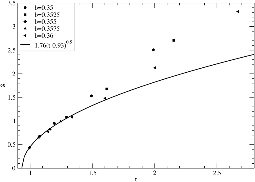
Figure 2: The gap in units of $T_{d}$ as a function of temperature in units of $T_{d}$.

7 No naive random matrix description.

Intuitively, one could argue that large $N_{c}$ alone, without the additional input from the viability of an effective chiral Lagrangian description is enough to motivate a random matrix description of spectral properties of the Dirac operator in planar QCD. If this were true, one ought to be able to describe the spectrum of the Dirac operator by some random matrix model even at temperatures where chiral symmetry is restored.

We tried to see if this is possible by looking at the correlation between the fluctuations of the lowest eigenvalues of the Dirac operator. These fluctuations are about the mean, so independent of the gap $g$, which is the main difference between the case where chiral symmetry is broken and we know that random matrix theory works and where we are when chiral symmetry is restored.

If indeed there is some random matrix model of the usual type considered the correlation between such fluctuations is mainly governed by level repulsion. We have two examples of such random matrix models: one where chiral symmetry is broken and the other where it is not, due to a large enough shift of $C$ (which occurs for $T$ large enough) in the formula for $D$ in equation 13.

We estimate by Monte Carlo methods the correlation, $c$ between the two lowest eigenvalues:

$$c=\frac{\langle(\lambda_{1}-\langle\lambda_{1}\rangle)(\lambda_{2}-\langle\lambda_{2}\rangle)\rangle}{\sqrt{\langle(\lambda_{1}-\langle\lambda_{1}\rangle)^{2}\rangle\langle(\lambda_{2}-\langle\lambda_{2}\rangle)^{2}\rangle}}$$ (18)

In the two random matrix models mentioned before $c$ is between $\frac{1}{2}$ (deep in the symmetric phase) and $\frac{1}{3}$ (broken phase). $c$ is bounded from above by 1 by a simple positivity argument. The numbers in table 1 show that $c$ is quite close to unity deep in the symmetric phase and and, although it drops down a little as the temperature decreases, $c$ remains well above $0.5$ even close to $t=1$. This indicates a much stronger correlation between the fluctuations of the lowest eigenvalues of the Dirac operator than one would expect in any random matrix model. The correlation we find is so strong as to imply an almost rigid relationship between the two lowest eigenvalues.

If there exists a random matrix model that applies to the case when chiral symmetry is restored, we are missing an essential ingredient, which we speculate might have something to do with the spectra of the eigenvalues associated with the Polyakov loops.

8 Comparison to holographic models.

Recently several papers discussing finite temperature features of models that bear various degrees of semblance to QCD have appeared [16, 17, 18]. These models are in the continuum, but admit dual descriptions which allow control of the strong coupling regime in the planar limit.

There are several models involving a set of branes which produce the gauge fields and the dual gravitational background and “probe” branes, that have no effect on the background, which produce the quark fields. One finds deconfining and chiral symmetry breaking transitions, all of first order.

In particular,  [18] addresses the issue of a chiral symmetry restoration transition in the supercooled deconfined phase and finds it is of first order. It seems that a crucial ingredient is the presence of an extra scale, beyond $\Lambda_{QCD}$, which allows for a more complex phase diagram. Nevertheless, it is noteworthy that some of these solvable situations are members of continuously varying families, which also contain ordinary QCD, albeit in a regime that is not under control in the dual variables.

Apart from the order of the transition in the supercooled phase, which admittedly is only tenuously determined here, there is general agreement between our findings here and the holographic results.

9 Conclusions

Our main conclusion is unsurprising: at infinite $N_{c}$ the strong first order deconfinement transition induces also immediate chiral symmetry restoration.

At a more minor level we obtained some less expected results: If we supercooled the deconfined phase chiral symmetry would still break spontaneously and seemingly does so in a continuous transition. Moreover, that transition would occur at a temperature which is only seven percent below the deconfinement transition. It is well known that such “pseudo-transitions” are indicative of complex dynamics even in the stable phase. We also saw that there is something fundamentally different in the statistics of the eigenvalues between the Dirac operator and typical random matrix theory models. It would be worthwhile to understand why this is so and what it means. In addition we were led to a heuristic explanation for why the coefficient $c$ in the free gas law for the free energy, $f=cT^{4}$, is weakly temperature dependent for temperatures close to $T_{d}$ and smaller than the classical value. The explanation viewed this as a consequence of the fact that the eigenvalues associated with the Polyakov loop are distributed over an arc of a certain width, and only at infinite temperature does the Polyakov loop become the trace of a matrix proportional to the unit matrix.

The new tools of holographic duals provide a wealth of exactly soluble strongly coupled theories where similar phenomena occur and it would be useful to find observables and models where both lattice and holographic methods apply simultaneously.

- [1] M. Teper, PoS LAT2005 (2005) 256, R. D. Pisarski, Phys. Rev. D29 (1984) 1222.
- [2] R. Narayanan, H. Neuberger, PoS LAT2005 (2005) 005.
- [3] R. Narayanan, H. Neuberger, Nucl. Phys. B696 (2004) 107.
- [4] T. D. Cohen, Phys. Rev. Lett. 93 (201601) 2004.
- [5] E.V. Shuryak and J.J.M. Verbaarschot, Nucl. Phys. A560 (1993) 306.
- [6] B. Lucini, M. Teper, U. Wenger, JHEP 0502 (2005) 033.
- [7] J. Kiskis, hep-lat/0507003.
- [8] M. A. Stephanov, Phys. Lett. B375 (1996) 249.
- [9] P. H. Damgaard, U. M. Heller, R. Niclasen, K. Rummukainen, Nucl. Phys. B583 (2000) 347.
- [10] A.D. Jackson and J.J.M. Verbaarschot, Phys. Rev. D53 (1996) 7223; T. Wettig, A. Schäfer and H.A. Weidenmüller, Phys. Lett. B367 (1996) 28; J.J.M. Verbaarschot, T. Wettig, Ann. Rev. of Nucl. and Particle Sci. Vol 50 (2000) 343.
- [11] J. Kiskis, R. Narayanan, H. Neuberger, Phys. Lett. B574 (2003) 65.
- [12] R. Narayanan, H. Neuberger, Nucl. Phys. B443 (1995) 305; H. Neuberger, Phys. Lett. B417 (1988) 141; H. Neuberger, Phys. Lett. B427 (1998) 353.
- [13] H. Neuberger, Nucl. Phys. Proc. Suppl. 73 (1999) 697.
- [14] J. L. Kapusta, Finite-temperature field theory, Cambridge Univ. Press (1989).
- [15] S. Coleman, E. Witten, Phys. Rev. Lett. 45 (1980) 100.
- [16] D. Mateos, R. C. Myers, R. M. Thomson, hep-th/0605046; T. Albash, V. Filev, C. V. Johnson, A. Kundu, hep-th/0605088; A. Karch, A. O’Bannon, hep-th/0605120.
- [17] A. Parnachev, D. A, Sahakyan, hep-th/0604173.
- [18] O. Aharony, J. Sonneschein, S. Yankielowicz, hep-th/0604161.