Lab/UFR-HEP0611/GNPHE/0611/VACBT/0611
QFT method for indefinite Kac-Moody Theory: A step towards classification

Abstract

We propose a quantum field theory (QFT) method to approach the classification of indefinite sector of Kac-Moody algebras. In this approach, Vinberg relations are interpreted as the discrete version of the QFT₂ equation of motion of a scalar field and Dynkin diagrams as QFT₂ Feynman graphs. In particular, we show that Dynkin diagrams of $su\left(n+1\right)$ series ($n\geq 1$) can be interpreted as free field propagators and $T_{p,q,r}$.diagrams as the vertex of $\phi^{3}$ interaction. Other results are also given.

Keywords: Vinberg theorem and KM theory, Dynkin diagrams, QFT Green functions, Feynman graphs.

1 Introduction

During last decade, the construction of four dimension (4D) supersymmetric quantum field theories (QFT₄) has attracted much attention in 10D superstring theory and D-brane physics [1, 2]. It has been investigated from various points; in particular in type II superstring models on Calabi-Yau (CY) manifolds with singularities classified by Dynkin diagrams of Lie algebras [3, 4, 5, 6]. The physics content of these stringy embedded super- QFTs is obtained from the deformation of these singularities and the D-branes wraping CY cycles. In this way, the physical parameters of the QFTs gets a wonderful interpretation; they are related to the moduli space of CY manifolds with ADE and conifold geometries [3, 7, 8]. This result is nicely obtained in the geometric engineering method by using mirror symmetry in CY geometries with K3 fibration. The ingredients of the super- QFT₄ (degrees of freedom, bare masses and gauge coupling constants, RG flows and cascades, superfields and their group representations,…) are remarkably encoded in quiver graphs similar to Dynkin diagrams of Kac-Moody (KM) algebras [3, 7, 8, 9, 10].

These developments have been made possible mainly due to the correspondence between supersymmetric quiver gauge theories and Dynkin diagrams of KM algebras. It has been behind the derivation of many (including exact) results in super- quantum field theories embedded in type II superstring models. Following [11], the correspondence between quiver gauge theories and Dynkin diagrams is a powerful tool which can be made more fruitful in both directions as indicated below:
(1) Use known results on Dynkin diagrams to extract much information on gauge theory embedded in type II superstring models as usually done in geometric engineering method:

$$Dynkin\text{ }diagrams\qquad\longrightarrow\qquad QFT.$$

This direction has been extensively explored in literature.
(2) Use standard methods of QFT to complete partial results on Kac-Moody algebras, in particular their classification and relation to extraordinary CY singularities beyond ordinary and affine ones:

$$QFT\qquad\longrightarrow\qquad Dynkin\text{ }diagrams.$$

The present study deals with the second direction. Note that at first sight, this project seems a little bit strange since generally one uses mathematics to approach physics; but here we are turning the arrow in the other way. Note also that despite almost four decades since their discovery in 1968, Kac-Moody extensions of simple Lie algebras [12] and their representations have not been fully explored in physics. If forgetting about unitarity for a while, this disinterest is also due to the lack of exact mathematical results with direct relevance for this matter. Only partial results have been obtained for the so-called KM hyperbolic subset. The indefinite sector of KM algebras is still an open problem in Lie algebra theory.

Motivated by results in type II string theory and its supersymmetric quiver gauge theory limit, we develop in his paper a QFT method to approach the classification of Dynkin diagrams of indefinite sector of KM algebras. Using this method, we show that:
(1) the QFT₂ equations of motion of a scalar field coincides, up to discretization, with the statement of Vinberg theorem. The latter is one of the basic ingredients in KM construction; it gives the classification of KM algebras into three major subsets.
(2) QFT₂ Feynamn graphs are interpreted as Dynkin diagrams.
In addition to above motivations, this field theoretic representation has moreover direct consequences on the following points:
(a) Shed more light on the striking similarity between Dynkin diagrams of KM extensions of semi simple Lie algebras and Feynman graphs of quantum field theory.
(b) Gives a new way to treat the theory of Lie algebras and their KM classification from physical point of view.
(c) Offers a new method to deal with the KM classification problem of Dynkin diagrams of indefinite sector of Lie algebras.
(d) Give more insight on the so called indefinite singularities of CY threefolds encountered in [9, 13, 16] and the corresponding indefinite quiver gauge sector.

The organization is as follows: In section 2, we review Vinberg theorem of classification of KM algebras and give the relation with QFT. In section 3, we propose a two dimensional QFT realization of Vinberg theorem and KM theory. In section 4, we give the physical representation of Vinberg condition requiring positivity of Vinberg vectors $\left(u_{i}\right)$. Last section is devoted to conclusion and discussions.

2  On Kac-Moody theory: Overview

In this section we give an overview on standard KM theory and preliminary results. Kac-Moody theory is just the extension of semi-simple Lie algebras of Cartan. The basis of this algebraic construction relies on the three following:
(1) Vinberg theorem of classification of square matrices $K$; in particular KM generalized Cartan matrices.
(2) Minimal realization of Vinberg matrices in terms of a triplet.
(3) Serre construction of Lie algebras using Chevalley generators.
Let us comment briefly these three algebraic steps. Roughly speaking, Vinberg theorem is a linear algebra theorem which applies to KM theory and beyond such as Borcherds algebras. This theorem states that the generalized Cartan matrices $K_{ij}$ (Cartan matrices for short) are of three kinds as shown here below

$$K_{ij}^{+}u_{j} > 0,$$

$$K_{ij}^{0}u_{j} = 0,$$ (2.1)

$$K_{ij}^{-}u_{j} < 0.$$

In these equations, $u_{j}$ are the positive numbers which will be discussed in section 4. The three upper indices $+$, $-$ and $0$ are conventional notations introduced in order to distinguish the three KM sectors. The rigorous statement of Vinberg theorem, as used in KM formulation, is as follows

Theorem 1

A generalized indecomposable Cartan matrix $\mathbf{K}$ obey one and only one of the following three statements:
(1) Finite type ( $\det\mathbf{K}>0$ ): There exist a real positive definite vector $\mathbf{u}$ ( $u_{i}>0;$ $i=1,2,...$) such that $\mathbf{K}_{ij}u_{j}=v_{j}>0$.
(2) Affine type, corank$\left(\mathbf{K}\right)=1$, $\det\mathbf{K}=0$: There exist a unique, up to a multiplicative factor, positive integer definite vector $\mathbf{n}$ ( $n_{i}>0;$ $i=1,2,...$) such that $\mathbf{K}_{ij}n_{j}=0$.
(3) Indefinite type ( $\det\mathbf{K}\leq 0$ ), corank$\left(\mathbf{K}\right)\neq 1$: There exist a real positive definite vector $\mathbf{u}$ ($u_{i}>0;$ $i=1,2,...$) such that $\mathbf{K}_{ij}u_{j}=-v_{i}<0$.

From the physical point of view, the first sector (ordinary class) of this KM classification deals with the ordinary semi simple Lie algebras. These algebras, which are familiar symmetries for model builders of elementary particle physics, are just the usual finite dimensional algebras classified many decades ago by Cartan (see figure 1). This model has been used in [3] to describe the geometric engineering of bi-fundamental matters

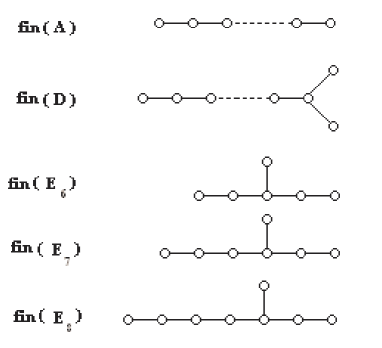
Figure 1: Dynkin diagrams of finite dimensional Lie algebras as classified by Cartan. These are graphs representing the usual ${\small\mathit{A}}_{n}\sim su\left(n+1\right)$ and ${\small\mathit{D}}_{n}\sim so\left(2n\right)$ classical simple Lie algebras as well as the ordinary exceptional ones. All of them have symmetric Cartan matrix K

The second class (affine class) of KM theory concerns affine Kac-Moody algebras. The latter plays a basic role in $2d$ conformal field theory (CFT₂) and underlying current algebras. These have been also used in the geometric engineering of $\mathcal{N}=2$ four dimensional conformal field theory embedded in Type II superstrings [16]. These infinite dimensional algebras were classified by Kac and Moody; see also figure 2.

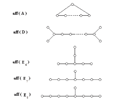
Figure 2: These are Dynkin diagrams of affine Kac-Moody extension of the corresponding ordinary ones given by figure (1). Like ordinary graphs, these diagrams are simply laced and symmetric Cartan matrix K  All these matrices have a vanishing determinant.

The third class (indefinite class) is the so-called KM indefinite class. In this sector, we dispose of partial results only; in particular for hyperbolic subset [13, 14, 15, 16, 17, 18], see also [19, 20, 21, 22].

Before going ahead, let us make two comments regarding the Vinberg relations (2.1). First, note that Vinberg relations as shown on theorem 1, are given by inequalities. However, they can be formulated as equations by introducing positive quantities $v_{i}$ (vectors) as follows:

$$K_{ij}^{\left(q\right)}u_{j}=qv_{i},\qquad q=+1,0,-1,$$ (2.2)

where the $\left(u_{i}\right)$s and $\left(v_{i}\right)$s are positive vectors. The second comment we want to make is that, because of the fact that any irreducible generalized Cartan matrix $K_{ij}^{\left(q\right)}$ can be decomposed as $A_{ij}-\delta A_{ij}^{\left(q\right)}$ with $\delta A_{ij}^{\left(q\right)}>0$, i.e

$$K_{ij}^{\left(q\right)}=A_{ij}-\delta A_{ij}^{\left(q\right)},$$ (2.3)

the above system of Vinberg equations may be also put in the following equivalent form

$$A_{ij}u_{j}=w_{i}\left(u\right),\qquad A_{ij}=\left(2\delta_{ij}-\delta_{i,j+1}-\delta_{i,j-1}\right),$$ (2.4)

where appears, on the left side, the ordinary $su\left(n\right)$ Cartan matrix $A_{ij}$ and where $w_{i}$ are some numbers whose physical meaning will be given when we consider our QFT realization.

Concerning the two other points (2) and (3) dealing with the algebraic construction of KM theory, the key idea of their content could be summarized as follows. Given a generalized Cartan matrix $K$, one can associate to it a KM algebra $g\left(K\right)$. This is achieved in two steps. First by using the minimal realization of Cartan matrix $K$ based on the usual triplet

$$\left(\hbar,\Pi,\Pi^{v}\right).$$ (2.5)

This triplet involves the following familiar objects: (i) Cartan subspace $\hbar$ with a bilinear form $<.,.>$ and a dual space $\hbar^{\ast}$, (ii) the root basis $\Pi=\left\{a_{i},\text{ \ \ }1\leq i\leq n\right\}\subset\hbar^{\ast}$ and (iii) the coroot basis $\Pi^{v}=\left\{a_{i}^{v},\text{ \ \ }1\leq i\leq n\right\}\subset\hbar$. In terms of these quantities, the Cartan matrix reads as

$$K_{ij}=<a_{i}^{v},a_{j}>,$$ (2.6)

which reads generally as $K_{ij}=2a_{i}a_{j}/a_{i}^{2}$. More conveniently, this can be taken as $K_{ij}=a_{i}a_{j}$ for simply laced KM algebras in which we will be interested in what follows. Note in passing that this algebraic formulation is not specific for Kac-Moody extension of semi simple algebras requiring

$$K_{ii} = 2,$$

$$K_{ij} < 0,\qquad i\neq j,$$ (2.7)

$$K_{ij} = 0\qquad\Rightarrow\qquad K_{ji}=0.$$

It is also valid for matrices beyond KM generalized Cartan ones. For instance, this above analysis applies as well for the case of Borcherds algebras using real matrices $\left(B_{ij}\right)$ constrained as

$$2\frac{B_{ij}B_{ji}}{B_{ii}}\in\mathbb{Z},\qquad B_{ii}\neq 0,\qquad B_{ij}\in\mathbb{R},$$ (2.8)

where $\mathbb{Z}$ is the set of integers. The third step in building KM algebra $g\left(K\right)$ is based on Chevalley generators $\left\{e_{i}\right\}$ and $\left\{f_{i}\right\}$, $i=1,..,n$. The Commutation relations of KM algebra $g\left(K\right)$ associated with a generalized Cartan matrix $K$ reads as follows

$$\begin{array}[]{l}\left[e_{i},f_{j}\right]=\delta_{ij}a_{i}^{\nu},\qquad 1\leq i,j\leq n\\ \left[h,h^{\prime}\right]=0,\qquad h,h^{\prime}\in\hbar\\ \left[a_{i}^{\nu},e_{j}\right]=K_{ij}e_{i},\\ \left[a_{i}^{\nu},f_{j}\right]=-K_{ij}f_{i}\text{,}\end{array}$$ (2.9)

together with Serre relations. In what follows, we shall develop a quantum field theoretical method to approach Vinberg theorem and KM theory describing the extension of semi simple Lie algebras. Our interest into this quantum field realization is motivated by a set of observations. Here, we list some of them:
(a) Dynkin diagrams of KM algebras have a remarkable similarity with the QFT Feynman graphs. For instance, Dynkin diagram of $A_{n}\simeq su\left(n+1\right)$ semi simple Lie algebra can be interpreted as a scalar QFT propagator. A naive correspondence reveals that the remaining known Dynkin diagrams are associated with a special class of QFT Green functions. It turns out that the Dynkin diagrams of less familiar KM algebras such as

$$T_{p,q,r}$$

hyperbolic algebras, with $p,q$ and $r$ positive integers greater than $2,$ have also a QFT counterpart. In particular, the $T_{p,q,r}$s (resp. $T_{p_{1},p_{2},p_{3},p_{4}}$) are formally analogous to the three (four) points tree vertex of scalar quantum field theory with a cubic (quartic) interaction.
(b) Cartan matrix $A$ of generic $su\left(n+1\right)$ algebras, with its very particular entries

$$A_{ij}=2\delta_{ij}-\delta_{i,j+1}-\delta_{i,j-1},$$ (2.10)

admits a special factorization, $A=P^{\dagger}P$. It turns out that its properties are quite similar to those of the $\left(1+1\right)$ dimensional Laplacian

$$\Delta=\frac{\partial^{2}}{\partial t^{2}}-\frac{\partial^{2}}{\partial x^{2}}=\partial_{+}\partial_{-}$$ (2.11)

of two dimensional QFT ( QFT₁₊₁). As we will see later, the $\left(A_{ij}\right)$ operator is noting but the discrete version of the Laplacian $\Delta$.
(c) The basis of classification of KM theory rests on Vinberg theorem relations namely $K_{ij}^{\left(+\right)}u_{j}>0,$ $K_{ij}^{\left(0\right)}u_{j}=0,\ K_{ij}^{\left(-\right)}u_{j}<0$ where the $K_{ij}$s are the KM generalized Cartan matrices. These relations, which can be also put in the compact form

$$K\left(z_{i},z_{j}\right)u\left(z_{j}\right)=v\left(z_{i}\right),$$ (2.12)

can be interpreted as quantum field equations of motion obtained from an action principle. Moreover, in a continuous scalar field $\Phi\left(t,x\right)$ interpretation, the right term $v\left(z_{i}\right)$ of above equation would be associated with $\frac{\partial W\left(\Phi\right)}{\partial\Phi\left(t,x\right)}$ evaluated at point $z_{i}$. Here $W\left(\Phi\right)$ is the interacting field potential. In this continuous QFT limit of Vinberg equations, one also sees that KM affine sector is associated with the critical points of the field potential $W\left(\Phi\right).$ This feature is in agreement with the general picture that we have about realization of KM affine symmetries and conformal invariance à la Sugawara.

3 QFT representation of Dynkin diagrams

To start note that a quantum field realization of Vinberg theorem can be naturally built by thinking about eq(2.4) as a $\left(1+1\right)$ dimensional field equation of motion resulting from the variation of the following discrete field action

$$\mathcal{S}\left[u\right]=\sum_{i,j\in\mathbb{Z}}\frac{1}{2}u_{i}A_{ij}u_{j}+\sum_{i\in\mathbb{Z}}W\left(u_{i}\right).$$ (3.1)

In this relation $u_{i}$ is as before, $A_{ij}=\left(2\delta_{ij}-\delta_{i,j+1}-\delta_{i,j-1}\right)$ and $W\left(u\right)$ is an interacting polynomial potential whose variation with respect to $u_{i}$ reads as follows

$$\frac{\partial W\left(u\right)}{\partial u_{i}}=w_{i}\left(u\right),$$ (3.2)

in agreement with eq(2.4). With this discrete field action at hand, one can go ahead and study quantization of this QFT by computing the generating functional $\mathcal{Z}\left[J\right]$ of Green functions of this theory,

$$\mathcal{Z}\left[J\right]=\int\left[Du\right]\exp\left(-\mathcal{S}\left[u\right]-\sum_{i}u_{i}J_{i}\right).$$ (3.3)

In this relation $\mathcal{S}\left[u\right]$ is as in eq(3.1) and the $J_{i}$s are the discrete values of an external source dual to the $u_{i}$s. The two points Green function (propagator) $G_{ij}=<u_{i},u_{j}>$ with $\left|i-j\right|=n,$ is interpreted as the Dynkin diagram of the $su\left(n+1\right)$ semi simple Lie algebra; see also figure 3.

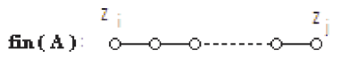
Figure 3: A generic Dynkin diagram of semi simple A_n Lie algebra realized as the two point function $<\Phi\left(z_{i},\overline{z}_{i}\right)\Phi\left(z_{j},\overline{z}_{j}\right)>$ with $n=1+\left|i-j\right|$.

More generally, Feynman graphs of the QFT eq(3.3) should be associated with Dynkin diagrams. We will not develop here the study of Green functions. What we want to do now is to establish the general setting of the QFT realization of KM theory and its relationship with $\left(1+1\right)$ dimensional continuous quantum scalar field theory.

Theorem 2

The Cartan matrix operator $A_{ij}=\left(2\delta_{ij}-\delta_{i,j+1}-\delta_{i,j-1}\right)$ of $su\left(n\right)$ semi simple Lie algebra is, up a multiplicative constant, exactly equal to the discrete version of the one dimensional laplacian operator $\Delta=\frac{d^{2}}{dx^{2}}$

$$\Delta\leftrightarrow\frac{1}{a^{2}}A_{ij},$$ (3.4)

where $a$ is period length of the discretized one dimensional lattice.
Vinberg theorem has a $\left(1+1\right)$ QFT realization; and Vinberg relations ($K_{ij}^{\left(+\right)}u_{j}>0,$ $K_{ij}^{\left(0\right)}u_{j}=0,\ K_{ij}^{\left(-\right)}u_{j}<0$) are given by the discretization of interacting field equations of motion, $A_{ij}u_{j}=\frac{\partial W\left(u\right)}{\partial u_{i}}$, with $\partial_{i}W\left(u\right)>0,$ $\partial_{i}W\left(u\right)=0$ and $\partial_{i}W\left(u\right)<0$ respectively

Before proving this theorem, let us introduce some tools and useful convention notations for our QFT realization of KM theory. First, let $\Psi\left(t,x\right)$ be a $\left(1+1\right)$ real scalar field of kinetic energy density

$$\mathcal{E}_{c}=\frac{\partial^{2}\Psi}{\partial t^{2}}-\frac{\partial^{2}\Psi}{\partial x^{2}}=\partial_{-}\partial_{+}\Psi.$$ (3.5)

Let also $\mathcal{R}\left(x\right)$ be a static real positive definite scalar field ($\mathcal{R}>0$ and $\frac{\partial\mathcal{R}}{\partial t}=0$) varying on the one dimensional real line $\mathbb{R}$. Because of stationarity, its kinetic energy density, given by a relation similar to the above one, reduces now to $\mathcal{E}_{c}=-\frac{d^{2}\mathcal{R}}{dx^{2}}$. In presence of field interactions $W\left(\mathcal{R}\right)$, the action $S=S\left[\mathcal{R}\right]$ of the scalar field model is given by

$$S\left[\mathcal{R}\right]=-\int_{\mathbb{R}}dx\left(\frac{1}{2}\left(\frac{d\mathcal{R}}{dx}\right)^{2}+W\left(\mathcal{R}\right)\right).$$ (3.6)

The continuous equation of motion of the real positive scalar field $\mathcal{R}$ reads as

$$\frac{d^{2}\mathcal{R}}{dx^{2}}=\frac{dW}{d\mathcal{R}},\qquad W\left(\mathcal{R}\right)=\sum_{m=1}^{n}\lambda_{m}\mathcal{R}^{m},$$ (3.7)

where $\lambda_{m}$ are coupling constants. To get the discrete version of this field equation, we use the correspondence $x\rightarrow x_{i}$ and $x+dx\rightarrow x_{i}+a$ and denote by

$$\mathcal{R}_{k}=\mathcal{R}\left(x\right)|_{x=x_{k}},\qquad k\in\mathbb{Z},$$ (3.8)

which is nothing but the field value at the node $x_{k}=ka$ of the one dimensional lattice $\mathbb{Z}$ with $a$ being the lattice period length.
We are now in position to prove our theorem. First, consider the discrete version of energy density $\left(\frac{d\mathcal{R}}{dx}\right)^{2}$. This is obtained by help of the usual definition of differentiation namely $\frac{d\mathcal{R}\left(x\right)}{dx}=\frac{\mathcal{R}\left(x+dx\right)-\mathcal{R}\left(x\right)}{dx}$ and by making the following substitutions

$$\mathcal{R}\left(x\right)\rightarrow\mathcal{R}_{i}\qquad\mathcal{R}\left(x+dx\right)\rightarrow\mathcal{R}_{i+1}.$$ (3.9)

Putting these expressions back into the continuous integral $\int_{\mathbb{R}}dx\left(\frac{d\mathcal{R}}{dx}\right)^{2}$, we get the discrete sum $\sum_{i\in\mathbb{Z}}\left(\mathcal{R}_{i+1}-\mathcal{R}_{i}\right)^{2}$ which expands as

$$\sum_{i\in\mathbb{Z}}\left(\mathcal{R}_{i+1}^{2}-\mathcal{R}_{i+1}\mathcal{R}_{i}\right)+\sum_{i\in\mathbb{Z}}\left(\mathcal{R}_{i}^{2}-\mathcal{R}_{i+1}\mathcal{R}_{i}\right).$$ (3.10)

Using translation invariance of the one dimensional lattice $\mathbb{Z}$, we can rewrite the first term of above equation $\sum_{i\in\mathbb{Z}}\left(\mathcal{R}_{i+1}^{2}-\mathcal{R}_{i+1}\mathcal{R}_{i}\right)$ as

$$\sum_{i\in\mathbb{Z}}\left(\mathcal{R}_{i}^{2}-\mathcal{R}_{i}\mathcal{R}_{i-1}\right).$$ (3.11)

This is achieved by shifting the indices as $\left(i+1\right)\rightarrow i$. The term $\sum_{i\in\mathbb{Z}}\left(\mathcal{R}_{i+1}-\mathcal{R}_{i}\right)^{2}$ reads then as $\sum_{i\in\mathbb{Z}}\left(2\mathcal{R}_{i}^{2}-\mathcal{R}_{i}\mathcal{R}_{i-1}-\mathcal{R}_{i+1}\mathcal{R}_{i}\right)$ and consequently we have the following continuous-discrete correspondence

$$\frac{1}{2}\int_{\mathbb{R}}dx\left(\frac{d\mathcal{R}}{dx}\right)^{2}\rightarrow\frac{1}{2a}\sum_{i,j\in\mathbb{Z}}\mathcal{R}_{i}A_{ij}\mathcal{R}_{j},$$ (3.12)

where $A_{ij}$ is exactly as given in theorem 2. The presence of the global factor $\frac{1}{a}$ in front of the discrete sum may be also predicted by using the following scaling properties of the scalar QFT under change $x\rightarrow ax$. In this way, we have

$$\mathcal{R}\left(x\right)\rightarrow\mathcal{R}\left(ax\right)=\mathcal{R}\left(x\right),\qquad W\left(\mathcal{R}\left(ax\right)\right)=\frac{1}{a^{2}}W\left(\mathcal{R}\left(x\right)\right)$$ (3.13)

This completes the proof of our theorem. What remains to do is to find the physical interpretation of the positivity condition of the $u_{i}$s in Vinberg theorem. This will be done in the next section.

4 Vinberg relations as field eq of motion

In Vinberg classification theorem of KM algebras (theorem 1), the $\left(u_{i}\right)$ variables eq(2.1) are required to be positive numbers. From physical point of view, such kind of conditions are familiar in the study of constrained systems; in particular in gauge theories. In the problem at hand, Vinberg condition may implemented by considering a static complex scalar QFT with a $U\left(1\right)$ gauge symmetry. To do so consider a QFT system composed by a static one dimensional gauge field $\mathcal{A}\left(x\right)$ ( a pure gauge field) and a complex scalar field $\Phi$

$$\Phi\left(x\right)=\frac{1}{\sqrt{2}}\left[\Phi_{1}\left(x\right)+i\Phi_{2}\left(x\right)\right].$$ (4.1)

For convenience, it is interesting to rewrite the field $\Phi$ by using Euler representation $\mathcal{R}\left(x\right)\exp i\vartheta\left(x\right)$ where the field $\mathcal{R}$ is same as before. Using the following $U\left(1\right)$ gauge transformations

$$\mathcal{R}\left(x\right) \rightarrow \mathcal{R}\left(x\right),$$

$$\vartheta\left(x\right) \rightarrow \vartheta\left(x\right)-\lambda\left(x\right),$$ (4.2)

$$\mathcal{A}\left(x\right) \rightarrow \mathcal{A}\left(x\right)-i\frac{d\lambda\left(x\right)}{dx}$$

where $\lambda\left(x\right)$ is the gauge parameter, and the gauge covariant derivative $\mathcal{D}=\frac{d}{dx}+i\mathcal{A}\left(x\right)$, one can write down the static one dimensional action $S\left[\Phi\right]$ describing the complex scalar field dynamics. It reads as,

$$S\left[\Phi\right]=-\int_{\mathbb{R}}dx\left[\left(\mathcal{D}\Phi\right)^{\ast}\left(\mathcal{D}\Phi\right)+W\left(\left|\Phi\right|\right)\right],$$ (4.3)

where $W\left(\left|\Phi\right|\right)=W\left(\mathcal{R}\right)$ is gauge invariant interacting potential, the same as in eq(3.6). Using gauge symmetry of this action, one can make the gauge choice

$$\vartheta\left(x\right)=\lambda\left(x\right),\qquad\mathcal{A}\left(x\right)=i\frac{d\lambda\left(x\right)}{dx},\qquad\mathcal{D}\Phi=\frac{d\mathcal{R}}{dx},$$ (4.4)

to kill the local phase $\vartheta\left(x\right)$ of the complex field $\Phi\left(x\right)$ which reduces then to $\mathcal{R}\left(x\right)$. Vinberg condition corresponds then to fixing the gauge field.

5 Conclusion and discussion

In this paper, we have developed the basis of a quantum field realization of KM theory of Lie algebras. As we know this structure, encoded by the Dynkin diagrams, play a central role in quantum physics and has been behind the developments of gauge theory and 2D critical phenomena.

In the case of simply laced Dynkin diagrams, we have shown that Vinberg theorem, classifying KM algebras, is in fact just the discrete version of the static field equation of motion

$$\frac{d^{2}\mathcal{R}}{dx^{2}}=\frac{dW\left(\mathcal{R}\right)}{d\mathcal{R}},\qquad\Phi=\mathcal{R}\exp i\vartheta,$$ (5.1)

following from the minimization of a complex scalar $U\left(1\right)$ gauge invariant theory. Gauge symmetry is used to fix the phase $\vartheta$ of the field $\Phi$ and the original field action $\mathcal{S}\left[\mathcal{R},\vartheta,\mathcal{A}\right]$ is left with only a dependence in the positive field $\mathcal{R}$. In this approach, Vinberg condition requiring positivity of the $u_{i}$s is interpreted as corresponding to the gauge fixing of $U\left(1\right)$ invariance eq(4.4). According to the sign of $\frac{dW}{d\mathcal{R}}$, one distinguishes then three sectors,

$$\frac{dW}{d\mathcal{R}} > 0,\qquad$$

$$\frac{dW}{d\mathcal{R}} = 0,\qquad$$ (5.2)

$$\frac{dW}{d\mathcal{R}} < 0.$$

In this representation, one sees that affine KM sector is associated with the critical point of the interacting field potential $W\left(\mathcal{R}\right)$ ($\frac{dW}{d\mathcal{R}}=0$). Semi simple Lie algebras are associated with

$$\frac{dW}{d\mathcal{R}}>0,$$ (5.3)

and interpreted as stable fluctuations around the critical point while indefinite symmetries related with unstable deformations,

$$\frac{dW}{d\mathcal{R}}<0.$$ (5.4)

In a subsequent study [23], we give other applications and more explicit details on this construction; in particular on the generating functional $\mathcal{Z}$ of Dynkin diagrams of KM algebras.

Acknowledgement 3

This research work is supported by the program protars III, CNRST D12/25. We thank R. Ahl Laamara, M. Ait Benhaddou and L.B Drissi for earlier collaboration on this matter.

References

- [1] A. Hanany, E. Witten, Type IIB Superstrings, BPS Monopoles, And Three-Dimensional Gauge Dynamics, Nucl. Phys. B492 (1997) 152-190, hep-th/9611230.
- [2] S. Katz, A. Klem, C. Vafa, Geometric engineering of quantum field theories, Nucl. Phys. B497(1997) 173, hep-th/9609239.
- [3] S. Katz, P. Mayr, C. Vafa, Mirror symmetry and Exact Solution of 4D Gauge Theories I, Adv.Theor.Math.Phys. 1 (1998) 53-114, hep-th/9706110.
- [4] R. Dijkgraaf, C. Vafa, A Perturbative Window into Non-Perturbative Physics, hep-th/0208048. On Geometry and Matrix Models, Nucl.Phys. B644 (2002) 21-39, hep-th/0207106.
- [5] F. Cachazo, S. Katz, C. Vafa, Geometric Transitions and Quiver Theories, hep-th/0108120.
- [6] F. Cachazo, K. Intriligator, C. Vafa, A Large N Duality via a Geometric Transition, Nucl.Phys. B603 (2001) 3-41, hep-th/0103067.
- [7] A. Belhaj, A. Elfallah, E.H. Saidi, On non simply laced mirror geometries in type II strings, Class.Quant.Grav.17(2000)515-532.
-
[8]
A. Belhaj, E.H. Saidi, Hyperkahler singularities in
Superstrings compactification and 2D CFTs,
Class.Quant.Grav. 18 (2001)57-82, hep-th/0002205,
A. Belhaj, E.H. Saidi, On Hyperkahler singularities, Mod.Phys.Lett.A15 (2000) 1767-1780, hep-th/0007143,
A. Belhaj, E.H Saidi, Toric geometry, enhaced nonsimply laced gauge symmetries in superstrings and F- theory, hep-th/0012131. - [9] M. Ait Ben Haddou, A. Belhaj, E.H. Saidi, Geometric Engineering of CFT4s based on Indefinite Singularities: Hyperbolic Case, Nucl.Phys. B674 (2003) 593-614, hep-th/0307244.
- [10] M. Ait Ben Haddou and E.H Saidi, Explicit analysis of Kahler deformations in supersymmetric quiver theories, Phys Lett B575(2003)100-110.
- [11] E.H Saidi, Notes on QFT representation of KM theory, Seminar given at the tenth workshop on the interface between High Energy and Mathematical Physics, Rabat, Mai 2005.
- [12] V.G. Kac, Infinite dimensional Lie algebras, third edition, Cambridge University Press (1990).
- [13] M. Ait Ben Haddou, A. Belhaj, E.H. Saidi, Classification of supersymmetric CFT4s: Indefinite Series, J. Phys A38 (2005), 1793-1806, hep-th/0308005.
- [14] E.H. Saidi, Hyperbolic invariance in type II superstrings, hep-th/0502176.
- [15] F. Cachazo, B. Fiol, K. Intriligator, S. Katz, C. Vafa, A Geometric Unification of Dualities, Nucl.Phys. B628 (2002) 3-78, Nucl.Phys. B628 (2002) 3-78.
- [16] R. Ahl Laamara, M. Ait Ben Haddou, A Belhaj, L.B Drissi, E.H Saidi, RG Cascades in Hyperbolic Quiver Gauge Theories, Nucl.Phys. B702 (2004)163-188 , hep-th/0405222.
- [17] P. Henry-Labordere, B. Julia, L. Paulot, Real Borcherds Superalgebras and M-theory, JHEP 0304 (2003) 060, hep-th/0212346.
- [18] M. Ait Ben Haddou, E.H Saidi, Hyperbolic Invariance, hep-th/0405251.
- [19] T. Damour, A. Hanany, M. Henneaux, A. Kleinschmidt, Hermann Nicolai, Curvature corrections and Kac-Moody compatibility conditions, hep-th/0604143.
- [20] C. Hillmann, A. Kleinschmidt, H. Nicolai, A note on gauge fixing in supergravity/Kac-Moody correspondences, hep-th/0603156.
- [21] S. Mizoguchi, K. Mohri, Y. Yamada, Five-dimensional Supergravity and Hyperbolic Kac-Moody Algebra G2H, hep-th/0512092.
- [22] L. Houart, Kac-Moody algebras in gravity and M-theories, hep-th/0511009.
- [23] A. Belhaj, E.H Saidi, Generating functional of Dynkin diagrams of KM algebras.