CERN-PH-TH/2006-091

IFT-UAM/CSIC-06-22

hep-th/0605166

We describe local Calabi-Yau geometries with two isolated singularities at which systems of D3- and D7-branes are located, leading to chiral sectors corresponding to a semi-realistic visible sector and a hidden sector with dynamical supersymmetry breaking. We provide explicit models with a 3-family MSSM-like visible sector, and a hidden sector breaking supersymmetry at a meta-stable minimum. For singularities separated by a distance smaller than the string scale, this construction leads to a simple realization of gauge mediated supersymmetry breaking in string theory. The models are simple enough to allow the explicit computation of the massive messenger sector, using dimer techniques for branes at singularities. The local character of the configurations makes manifest the UV insensitivity of the supersymmetry breaking mediation.

1 Introduction

The study of low energy supersymmetry and supersymmetry breaking are the main driving forces in present research in physics beyond the Standard Model. Hence, their description and understanding in terms of an underlying theory is highly desirable.

String theory implements supersymmetry at high energies automatically, and has enough richness to allow for mechanisms of supersymmetry breaking, and its mediation to the Standard Model sector. A nice scenario is supersymmetry breaking in a hidden sector with gravity mediation, and a particularly nice realization is in flux compactifications (see [1, 2, 3, 4], etc), with the moduli acting as hidden sector. In this particular setup, techniques to obtain the soft terms have been devised [5, 6, 7, 8, 9, 10, 11, 12, 13], (some exploiting earlier model-independent approaches [14, 15, 16]).

Gauge mediated supersymmetry breaking (GMSB) is a purely field theoretical mechanism of supersymmetry breaking mediation, insensitive to UV dynamics (and hence to gravity). Still it is important to understand its realization in a complete theory like string theory. This requires the construction of string theory configurations with gauge sectors whose (presumably strong) dynamics is under control. Hence we may expect great benefits from recent developments in the understanding of gauge theory dynamics in D-brane setups, mainly motivated by the gauge/string correspondence. For instance, the study of configurations of D3-branes at singularities, in the presence of fractional branes, has led to the realization of large classes of gauge theories with strong infrared dynamics, giving rise to interesting phenomena like different patterns of confinement [17, 18] (by the so-called deformation fractional branes), or the removal of the supersymmetric vacuum [19, 20, 21] (by the so-called DSB fractional branes) .

In fact, the latter configurations were explicitly used in [26] in the construction of string compactifications with semi-realistic visible sectors and a sector of DSB branes. These are the first serious attempts to implement GMSB in string theory.

In this paper we continue along those lines, improving it in several directions. We propose a fairly general framework to discuss models of GMSB in string theory. The construction is based on the use of local (namely non-compact) configurations, with two sectors of D-branes describing the visible and supersymmetry breaking sector, decoupled at the massless level, but coupled via a messenger sector whose mass scale is controlled by the distance between the D-brane sectors, which is much smaller than the string scale. In fact, it is this latter fact that motivates considering local configurations, since the physics of the mediation is naturally insensitive to the global structure of the compactification . We propose explicit realizations of this construction, which is nevertheless quite flexible and allows for many generalizations.

Some of the nice features of our proposal and explicit models are:

$\bullet$ Being local, they manifestly show the UV insensitivity of the construction.

$\bullet$ As opposed to previous proposals, the computation of the spectrum and interactions of the messenger sector can be explicitly described.

$\bullet$ The construction is simple and flexible enough to allow for many generalizations.

We find that these nice features are an important step in improving models of GMSB in string theory.

Our constructions are based on local Calabi-Yau geometries with two isolated singularities, at which sectors of D-branes are located. In the construction of the geometries and the determination of the gauge sector, we invoke important recent developments on D-branes at singularities, especially dimer diagrams (or brane tilings) [27, 28, 29, 30, 31, 32], which we review in order to make the paper self-contained. The location of the D-branes at singularities is a natural way to obtain chiral 4d $N=1$ gauge theories, rich and flexible enough to allow for semi-realistic sectors and sectors with supersymmetry breaking dynamics. In particular, we can construct examples where the visible sector is an MSSM like model with the Standard Model gauge factors and 3-families of quarks and leptons, introduced in [33], and the supersymmetry breaking sector is provided by the flavored $dP_{1}$ models in [24]. Implementation of other concrete models in our framework is possible as well, and we mention several possible generalizations (in particular, we discuss how to include in our setup models with visible sectors based on non-abelian orbifold singularities, like $\bf C^{3}/\Delta_{27}$ [33, 34, 35]).

The paper is organized as follows. In Section 2 we provide background material on dimer diagrams: Section 2.1 describes the gauge theories on configurations of D3- and D7-branes at singularities using the tools from dimer diagrams. Section 2.2 reviews the construction of gauge theories with supersymmetry breaking using D-branes. Section 2.3 describes the construction of local CY models with several separated singularities, by using partial resolution.

In Section 3 these tools are put to work in the construction of a simple local CY with two sectors, corresponding to D3-branes at two separated singularities. One D3-brane stack describes the visible sector (in a toy version given by a 3-family $SU(3)^{3}$ trinification model) while the other describes the supersymmetry breaking sector (although it actually corresponds to a theory with a runaway behaviour). In Section 3.2 a more complete model is presented, based on the previous model with the addition of D7-branes. The visible sector is given by a 3-family MSSM-like theory, while the hidden sector breaks supersymmetry in a local metastable minimum. Such explicit constructions are amenable to the study of several phenomenological questions. In Section 4 we sketch other model building possibilities. Finally in Section 5 we present some final remarks. The computation of the massive messenger sector in this general class of models is presented in Appendix A.

2 Background material

2.1 D-branes at singularities and dimer diagrams

D3-branes at singularities

Systems of D3-branes at singularities have been under intense study from the viewpoint of the AdS/CFT correspondence (starting with [36], see [37, 38, 39, 40, 41, 42] for some recent references) and extensions to related non-conformal systems (see e.g. [17, 43, 44, 18, 19, 20, 21]).

Another useful viewpoint on these systems is to consider them local models of interesting gauge/D-brane dynamics, often illustrating properties of more general configurations. In particular, they can be regarded as a local description of a global compactification, in a regime where the relevant D-branes are close to each other, as compared with the compactification scale. This is the viewpoint we take in the present paper, in the spirit of [33].

A recent useful tool in the study of D3-branes at singularities is provided by the dimer diagrams or brane tiling [27, 28, 29, 30], which we review in this Section.

D3-branes located at a singularity in the transverse space lead to 4d gauge theories in their world-volume. For Calabi-Yau singularities, these theories are $N=1$ and are characterized by a set of gauge factors, chiral multiplets in bi-fundamental representations, and superpotential interactions among them. This structure is nicely encoded in the so-called dimer diagrams (or brane tilings) [27, 28, 29, 30, 31]. They correspond to a periodic tiling of $\bf R^{2}$ or equivalently a tiling of the 2-torus $\bf T^{2}$. In order to correspond to a gauge theory on D3-branes at a singularity, there are further constraints on the tiling. The main one is that the graph should be bi-partite, namely the nodes can be colored with two colours (black and white), with edges joining nodes of different color. We skip further discussions, and refer the reader to e.g. [28, 29] for details.

In this language, each face corresponds to a gauge factor, each edge separating two faces corresponds to a chiral multiplet in the bi-fundamental representation, and each node corresponds to an interaction term in the superpotential, involving the bi-fundamentals corresponding to the edges ending on that node . Note that the orientation on the edges (e.g. from black to white nodes) must be used to define the bi-fundamentals. Also, superpotential terms associated to black or white nodes have opposite signs.

One example, corresponding to D3-branes at the $\bf C^{3}/\bf Z_{3}$ singularity (also known as the complex cone over $dP_{0}$, hence denoted $dP_{0}$ singularity in the following), is shown in Figure 1a. The gauge theory corresponding to the dimer diagram in Figure 1a is described in Figure 1b in terms of its quiver diagram, where nodes correspond to gauge factors, arrows correspond to chiral multiplets, and the superpotential needs to be specified explicitly. In this case we have

$$W = {\rm Tr\,}\,(\,X_{12}Y_{23}Z_{31}\,-\,X_{12}Z_{23}Y_{31}\,+\,X_{23}Y_{31}Z_{12}\,-\,X_{23}Z_{31}Y_{12}\,+$$ (2.1)

$$+ X_{31}Y_{12}Z_{23}\,-\,X_{31}Z_{12}Y_{23}\,)\,\simeq\,\epsilon_{ijk}\,{\rm Tr\,}(\,X_{12}^{(i)}X_{23}^{(j)}X_{31}^{(k)}\,)$$

with obvious notation (in the last expression we have written $X^{(i)}$, $i=1,2,3$ for $X$, $Y$, $Z$, respectively). Traces in superpotential terms will be implicit in what follows.

Figure 1: (a) The dimer diagram (as a tiling of the $\bf T^{2}$ upon identifying sides of the paralelogram) and (b) the quiver diagram of the gauge theory on D3-branes at the $\bf C^{3}/\bf Z_{3}$ singularity.

For completeness and future use, we show another example of a dimer diagram in Figure 2a, corresponding to D3-branes at a singularity given by the complex cone over $dP_{1}$ (in what follows, $dP_{1}$ singularity for short). The corresponding gauge theory (denoted $dP_{1}$ theory) is described by the quiver diagram shown in Figure 2b, with the superpotential given by

$$W = X_{12}Y_{24}X_{41}\,-\,Y_{12}X_{24}X_{41}\,+\,X_{31}Y_{12}X_{23}\,-$$ (2.2)

$$- Y_{31}X_{12}X_{23}\,+\,Z_{12}X_{24}X_{43}Y_{31}\,-\,Z_{12}Y_{24}X_{43}X_{31}\,$$

$$\simeq \epsilon_{ij}X_{12}^{i}X_{24}^{j}X_{41}\,+\,\epsilon_{ij}X_{31}^{i}X_{12}^{j}X_{23}\,+\,\epsilon_{ij}Z_{12}X_{24}^{i}X_{43}X_{31}^{j}$$

where fields $X^{i}$, $i=1,2$ denote $X$, $Y$.

Figure 2: The dimer diagram (a) and quiver diagram (b) of the gauge theory on D3-branes at a singularity given by a complex cone over $dP_{1}$ (the $dP_{1}$ theory, for short).

Dimer diagrams have been shown to encode the string theory geometry in several ways. In the following we provide the most practical description for our purposes.

A toric Calabi-Yau geometry is characterized by its web diagram, see [45, 46, 47] for a first application in the physical context and e.g. [18] for applications to systems of D3-branes . The web diagram for a toric singularity is given by a set of segments in $\bf R^{2}$, carrying $(p,q)$ labels which define their orientation . Segments join at vertices, with the rule that the $(p,q)$ charges of segments at a vertex add up to zero.

The web diagram for the $\bf C^{3}/\bf Z_{3}$ ($dP_{0}$) and the $dP_{1}$ singularities are shown in Figures 3a and 4a. The web diagram can be regarded as describing the locus where certain $\bf S^{1}$ fibrations in the toric geometry degenerate. Skipping the details, this description implies that finite size segments and faces correspond to 2-cycles and 4-cycles respectively. External legs and non-compact faces correspond to non-compact 2- and 4-cycles. The structure of the singularity is specified by the set of $(p,q)$ charges of the external legs, while the sizes of the internal finite size pieces simply corresponds to a choice of Kahler moduli. The singular variety corresponds to shrinking the finite pieces to a point.

Figure 3: (a) Web diagram for the $dP_{0}$ singularity. For clarity we show the geometry for a non-zero size of the internal pieces. (b) Dimer diagram and zig-zag paths for the $dP_{0}$ theory. The $(p,q)$ homology class of the path is related to the $(p,q)$ label of an external leg in the web diagram of the geometry.

Figure 4: (a) Web diagram for the $dP_{1}$ singularity. For clarity we show the geometry for a non-zero size of the internal pieces. (b) Dimer diagram and zig-zag paths for the $dP_{1}$ theory. The $(p,q)$ homology class of the path is related to the $(p,q)$ label of an external leg in the web diagram of the geometry.

The dimer diagram for the gauge theory on D3-branes at a singularity encodes the $(p,q)$ charges of the external legs in the corresponding web diagram [29, 30], in its structure of zig-zag paths. A zig-zag path is a path made of dimer edges, such that it turns maximally to the left at e.g. black vertices and maximally to the right at white vertices. Each zig-zag path defines a closed loop on $\bf T^{2}$, and carries a non-trivial $(p,q)$ homology charge. Each zig-zag path corresponds to an external leg in the web diagram, with the $(p,q)$ label of the leg given by the $(p,q)$ charge of the path. It is easy to recover the web diagrams of different singularities from the zig-zag paths of the dimer diagram, as the reader can check in our examples. The structure of zig-zag paths for the $dP_{0}$ and $dP_{1}$ dimer diagrams are shown in Figures 3b and 4b.

We would like to mention a more advanced concept, the mirror Riemann surface $\Sigma$ and its relation to the dimer. This is useful in the derivation of some results, although we will always provide the final answers in a language not involving it, so that the reader can safely skip them (we refer to [30] for further details). The web diagram of a toric singularity can also be regarded as a skeleton for a Riemann surface $\Sigma$ with punctures, which is obtained by ‘thickening’ the segments to tubes. Punctures in $\Sigma$ correspond to external legs in the web diagram. This Riemann surface plays a prominent role in the description of the mirror geometry, and all relevant D-branes are described as wrapped on 1-cycles on it. In particular, the D3-brane gauge factors correspond to non-trivial compact 1-cycles in $\Sigma$. The number of intersections (counted with orientation) between two such 1-cycles gives the number of bi-fundamentals between the corresponding gauge factors. Finally, the superpotential terms correspond to disks in $\Sigma$ bounded by pieces of different 1-cycles. Although this picture underlies the derivation of our tools, we rephrase the results directly in terms of the dimer diagram

Adding D7-branes

For certain applications, it is desirable to introduce D7-branes passing through a system of D3-branes at a singularity. Namely, one introduces D7-branes wrapped on holomorphic 4-cycles of the singular CY. From the viewpoint of the 4d gauge theory, this implies the introduction of a set of flavours for the different D3-brane gauge factors (from the open strings between the D3- and D7-branes) and interactions (e.g. from 73-33-37 interactions). Notice that the gauge group on the D7-branes behaves as a global symmetry from the viewpoint of the 4d gauge theory in this non-compact setup.

It turns out that the introduction of such D7-branes can be easily described in the language of dimer diagrams, in a manner that allows reading off the D3-D7 spectrum and interactions. This has been described in appendix B of [24], whose results we briefly review. Using the mirror Riemann surface $\Sigma$ mentioned above, D7-branes are represented as non-compact 1-cycles in $\Sigma$ that stretch between two punctures. The intersections of the D7-brane 1-cycle with the 1-cycle corresponding to the D3-branes gives rise to chiral multiplets in bi-fundamentals of the D3- and D7-brane symmetry groups, thus providing the D3-D7 spectrum. Finally, disks in $\Sigma$ bounded by one D7-brane 1-cycle and two D3-brane 1-cycles lead to a cubic superpotential term of the form 73-33-37. This more detailed description underlies our above recipe, which we nevertheless can state directly in terms of the dimer diagram.

As described in [24], for each 33 bi-fundamental in the D3-brane sector, there exists one kind of D7-brane leading to 37, 73 chiral multiplets coupling to the 33 state. Hence, a simple representation of a D7-brane in the dimer diagram is as a segment stretching across an edge, joining the mid-points of adjacent faces. One such segment stretching across an edge associated with an $(\raisebox{-0.5pt}{\hbox{\rule{0.4pt}{6.5pt}\hskip-0.4pt\rule{6.5pt}{0.4pt}\hskip-6.5pt\rule[6.5pt]{6.5pt}{0.4pt}}\rule[6.5pt]{0.4pt}{0.4pt}\hskip-0.4pt\rule{0.4pt}{6.5pt}}_{1},\overline{\raisebox{-0.5pt}{\hbox{\rule{0.4pt}{6.5pt}\hskip-0.4pt\rule{6.5pt}{0.4pt}\hskip-6.5pt\rule[6.5pt]{6.5pt}{0.4pt}}\rule[6.5pt]{0.4pt}{0.4pt}\hskip-0.4pt\rule{0.4pt}{6.5pt}}}_{2})$ bi-fundamental, gives rise to chiral multiplets in the $(\raisebox{-0.5pt}{\hbox{\rule{0.4pt}{6.5pt}\hskip-0.4pt\rule{6.5pt}{0.4pt}\hskip-6.5pt\rule[6.5pt]{6.5pt}{0.4pt}}\rule[6.5pt]{0.4pt}{0.4pt}\hskip-0.4pt\rule{0.4pt}{6.5pt}}_{2};\overline{N_{D7}})$ and $(N_{D7};\overline{\raisebox{-0.5pt}{\hbox{\rule{0.4pt}{6.5pt}\hskip-0.4pt\rule{6.5pt}{0.4pt}\hskip-6.5pt\rule[6.5pt]{6.5pt}{0.4pt}}\rule[6.5pt]{0.4pt}{0.4pt}\hskip-0.4pt\rule{0.4pt}{6.5pt}}}_{1})$, where $N_{D7}$, $\overline{N_{D7}}$ represent the D7-brane global symmetries. Heuristically, the D7-brane segment touches the faces at its endpoints, leading to the D7-D3 and D3-D7 sectors according to orientation. There is a superpotential coupling 33-37-73 involving these states. The representation as a segment facilitates an easy identification of the gauge theory matter content and interactions corresponding to a system of D3- and D7-branes at singularities. In Figure 5 we show one particular example of this kind of diagram, which we denote extended dimer diagram. Notice that there are other possible D7-brane choices, namely one for each 33 bi-fundamental, and that for different 33 bi-fundamentals with the same gauge quantum numbers, the corresponding D7-branes lead to the same 37, 73 spectrum, but different 33-37-73 interactions.

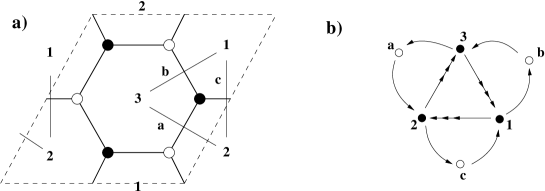
Figure 5: (a) Extended dimer diagram of the $dP_{0}$ theory with some examples of D7-branes represented as segments across the edges. (b) Quiver diagram including D7-branes (represented as white nodes). There are 33-37-73 couplings involving the 33 bi-fundamental across which the corresponding D7-brane stretches.

An important point is that there are non-trivial consistency conditions on configurations of D3- and D7-branes at singularities. Concretely, the total charge of the D-brane system under RR fields living at the singular points should vanish. Equivalently [48, 49, 50], the 4d gauge theory should be free of non-abelian anomalies . In all our forthcoming examples we enforce this property.

One can use these tools to construct interesting gauge theories. As a particular application to phenomenological model building, it is easy to construct configurations leading to MSSM like spectra [33]. In Figure 6a we show an extended dimer diagram for a system of D3- and D7-branes at a $\bf C^{3}/\bf Z_{3}$ singularity studied in [33]. As can be easily read out from the picture, it leads to a $U(3)\times U(2)\times U(1)$ gauge group and 3-families of quarks and leptons (plus additional fields, with vector-like quantum numbers under the Standard Model gauge group). The only massless $U(1)$ linear combination (in a convenient normalization) is $Q_{Y}=-\frac{1}{2}(\frac{1}{3}Q_{3}+\frac{1}{2}Q_{2}+Q_{1})$. This is crucial, since it precisely reproduces the correct hypercharges of the matter fields. In Figure 6b we show the quiver diagram for this gauge theory , with arrows labeled by the corresponding (Minimal Supersymmetric) Standard Model field. Notice that, in contrast with the MSSM, the model contains a triplicated sector of Higgs fields, and also that there are three copies of fields, vector-like under the D3-brane gauge interactions, with quantum numbers of $D_{R}$ quarks (and conjugates $\overline{D_{R}}$). See [33] for further details. In later sections, we will use this configuration as our (toy) model for the visible sector in a truly realistic string compactification.

\psfrag{QL}{$Q_{L}$}\psfrag{UR}{$U_{R}$}\psfrag{DR}{$D_{R}$}\psfrag{DRb}{$\overline{D_{R}}$}\psfrag{L}{$L$}\psfrag{E}{$E$}\psfrag{HU}{$H_{U}$}\psfrag{HD}{$H_{D}$}\includegraphics[scale={0.50}]{dp0mssm.eps}

Figure 6: Dimer diagram (a) and quiver diagram (b) for a configuration of D3/D7-branes realizing a gauge theory close to the MSSM.

2.2 DSB from D-branes at singularities

An interesting spinoff in the study of D-branes at singularities has been the realization of gauge theories whose non-perturbative dynamics removes the supersymmetric vacuum [19, 20, 21]. The prototypical example is provided by the gauge theory on a set of fractional branes on the $dP_{1}$ singularity. Moreover, the same behaviour is found in many other examples, and can in fact be argued to be generic. Nevertheless let us concentrate on the $dP_{1}$ case for concreteness (and for future application to our main examples).

The general gauge theory for D3-branes at a $dP_{1}$ singularity has been described in Section 2.1. Consider the particular situation where

$$N_{4}=0\quad,\quad N_{1}=M\quad,\quad N_{2}=2M\quad,\quad N_{3}=3M,$$ (2.3)

which corresponds to an anomaly-free, and hence consistent, choice. Recalling that the $U(1)$ gauge factors are massive (see footnote 6), the gauge group is $SU(3M)\times SU(2M)\times SU(M)$. The superpotential reads

$$W = \,X_{23}X_{31}Y_{12}\,-\,X_{23}Y_{31}X_{12}$$ (2.4)

In addition there is the field $Z_{12}$, decoupled at this level. As discussed in [19, 20, 21] (see [22] for a detailed discussion), in the regime where the $SU(3M)$ dynamics dominates this gauge factor confines and develops an Affleck-Dine-Seiberg (ADS) superpotential for its mesons $M_{21}=X_{23}X_{31}$, $M_{21}^{\prime}=X_{23}Y_{31}$. The complete superpotential is

$$W = M_{21}Y_{12}\,-\,M_{21}^{\prime}X_{12}\,+\,M\,\left(\,\frac{\Lambda_{3}^{7M}}{\det{\cal M}}\,\right)^{\frac{1}{M}}$$ (2.5)

where ${\cal M}=(M_{21};M_{21}^{\prime})$ is the mesonic $2M\times 2M$ matrix. The theory has no supersymmetric vacuum since the F-term conditions for $X_{12}$, $Y_{12}$ send $M_{21},M_{21}^{\prime}\to 0$, and then the F-terms conditions for $M_{21}$, $M_{21}^{\prime}$ send $X_{12},Y_{12}\to\infty$. In fact, assuming canonical Kahler potential for the matter fields, one easily shows there is a runaway behaviour towards this minimum ‘at infinity’ [20, 22]. The runaway direction is parametrized by the gauge-invariant dibaryonic operator

$$\epsilon^{a_{1}\ldots a_{2M}}\epsilon^{b_{1}\ldots b_{M}}\epsilon^{c_{1}\ldots c_{M}}(X_{12})_{b_{1}a_{1}}\ldots(X_{12})_{b_{M}a_{M}}(Y_{12})_{c_{1}a_{M+1}}\ldots(Y_{12})_{c_{M}a_{2M}}$$ (2.6)

As mentioned above, this pattern is generic for a large class of systems of D-branes at singularities. Namely, for the so-called DSB fractional branes [20], see [23] for the gauge theory analysis in a large set of examples.

It is useful to mention an equivalent viewpoint on the runaway [20]. The $U(1)$ gauge factors can be maintained in the gauge theory, as long as one consistently includes the $B\wedge F$ couplings (and its supersymmetry related coupling of the NSNS scalar $\phi$ partner of $B$ as a Fayet-Iliopoulos (FI) term) in the dynamics, see footnote 6. Considering the FI $\phi$ for the linear combination $Q_{1}-Q_{2}$ of the $U(1)$’s in $U(M)\times U(2M)$, there is a non-trivial D-term constraint for fixed FI $\phi$, roughly of the form

$$V_{D}\,=\,(\,|X_{12}|^{2}+|Y_{12}|^{2}+\phi\,)^{2}$$ (2.7)

From this viewpoint, at fixed values of $\phi$ the D-term for the $U(1)$ lifts the runaway direction and leads to a non-supersymmetric minimum. In the complete theory, however, the FI term is actually a dynamical field $\phi$, which can decrease the vacuum energy to arbitrarily low values by relaxing to infinity. Hence the runaway behaviour is recovered, now in terms of the closed string mode $\phi$ .

This behaviour is interesting, but in principle it would seem of little phenomenological interest as a mechanism for supersymmetry breaking. However, it has recently been shown in [24] that upon a small modification, the above class of theories (in particular the $dP_{1}$ theory) contain supersymmetry-breaking local minima, which are metastable and long-lived, since they are separated from the runaway behaviour at infinity by a large potential barrier . The modification is a remarkably simple generalization of the proposal in [25] for SYM theories. It is provided by the introduction of massive flavours, with masses much smaller than the dynamical scale of the gauge theory. The additional flavours can be easily incorporated by the introduction of D7-branes in the system of D3-branes at singularities. We refer the reader to [24] for details on the string construction and the gauge theory analysis of this theory .

In Figure 7 we show the extended dimer diagram corresponding to the system of D3- and D7-branes (with the rank assignment (2.3) and $2M$ D7-branes). Other possible choices of D7-branes can in principle be similarly considered. In coming Sections we will use this configuration as a basic model of a sector leading to dynamical supersymmetry breaking (in its local non-supersymmetric minimum).

Figure 7: (a) Dimer diagram for a configuration of D3- and D7-branes in the $dP_{1}$ singularity leading to a gauge theory with meta-stable supersymmetry breaking vacua. (b) Extended quiver diagram for the theory.

An alternative possibility to obtain stable non-supersymmetric minima from DSB branes, already mentioned in [26] is the following. As mentioned above, the runaway behaviour can be regarded as a non-trivial potential for a certain Kahler modulus of the singularity. In global compactifications, it is possible that there are other sources of potential for these moduli, which could presumably stabilize its runaway (for instance non-perturbative contributions arising from euclidean D3-brane instantons). This is however difficult to verify in concrete models including realistic sectors etc. Moreover, the properties of such local minima (including its very existence) would be strongly sensitive to the details of the global compactification. This goes against our strategy to attempt the construction of a visible plus DSB sector with no UV sensitivity.

In other words, one can rephrase the above by saying that in our specific local models, which are UV insensitive by construction, there are no other sources of potential for the Kahler moduli involved in the runaway. Hence, the above proposal to modify the gauge theory by adding slightly massive flavours is a UV independent way to generate supersymmetry breaking minima in these gauge theories, and a natural one to be implemented in local models.

2.3 Local CY models with several singularities

Geometrical construction from partial resolution

In this last subsection we would like to describe the construction of the geometries of our interest, namely local Calabi-Yau varieties with two isolated singularities, and the gauge theories for D-branes placed on them. This is based on tools developed in [32].

As mentioned above, non-compact toric Calabi-Yaus can be characterized using web diagrams. In this language, the construction of local CYs with two isolated singularities is straightforward, by the procedure of partial resolution. We start with a web diagram describing a geometry with a single singular point, namely all finite segments and faces are collapsed to a point at which all external legs converge. Now we grow one finite size segment out of such a point. The web diagram now has two internal vertices at which external legs converge. This implies that the geometry now has two singular points, separated by a distance controlled by the Kahler modulus of the 2-cycle corresponding to the finite segment. The ideas are better illustrated using a concrete example. Hence, we consider an example studied in [32], namely the splitting of the so-called double conifold singularity (studied in [54, 55]) to two conifold singularities. The web diagram for this singularity is shown in Figure 8a, and a partial resolution is illustrated in Figure 8b.

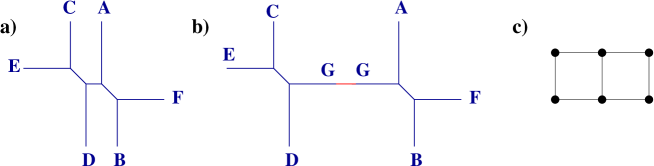
Figure 8: (a) The web diagram for the double conifold singularity $xy=s^{2}w^{2}$. (b) The partial resolution to a geometry with two conifold singularities. (c) Description in terms of the toric diagram.

The geometry of the two daughter singularities can be studied by considering all legs entering the corresponding vertex (including the finite size segment). Namely, by breaking the finite segment we obtain two daughter web diagrams which describe the local geometry around the two daughter singularities . This is manifest in Figure 8b, where, upon breaking the elongated segment (by removing the red piece in Figure 8b) we are left with two web diagrams describing the two conifold singularities in the left-over geometry. Notice that the original and final singularities are simpler to recognize if one keeps track of the collapsed finite segments, by showing them with a small size, as we do in all our discussions. Recall however that the singularities are obtained when such finite pieces have zero size.

Notice that this process can be easily inverted. If one is interested in constructing a local CY with two isolated singularities of specified type, one simply needs to consider combining their web diagrams into a larger one by joining one external leg of each diagram into one finite size segment . This will be useful in the construction of geometries in Section 3.

Finally let us mention that the partial resolution, when regarded in terms of the mirror Riemann surface $\Sigma$, simply corresponds to elongating a tube. By pinching this tube (or elongating it infinitely) one obtains two daughter Riemann surfaces that describe the mirror of the two daughter singularities.

2.3.1 Effect on D-branes

We would like to describe the effect of the above partial resolutions on systems of D-branes at the original singularity. This is most easily determined using the language of dimer diagrams in previous Sections.

For D3-branes, this has been systematically described in [32], which we review in what follows. Consider the gauge theory on D3-branes at the initial singularity. Following the proposal in [52], the partial resolution corresponds to giving a vev to a closed string Kahler modulus. This couples as a FI term for the $U(1)$ gauge fields in the D3-brane gauge theory, which therefore forces a set of bi-fundamental multiplets to acquire a vev, breaking the gauge group by a Higgs mechanism. After the Higgs mechanism, one recovers two gauge sectors, which are decoupled at the level of massless states, and which represent the gauge theory on D3-branes at the two daughter singularities. The massive states correspond to the massive open strings stretching between D3-branes at different singularities. In the case where the two gauge sectors correspond to the visible and supersymmetry breaking sectors, the massive modes are the messengers of supersymmetry breaking.

The above discussion can be made very explicit using the dimer diagrams. Consider the dimer diagram describing the gauge theory on D3-branes at the initial singularity. As discussed above, the zig-zag paths of the dimer diagram correspond to the external legs of the initial web diagram. When the partial resolution is carried out, the web diagram splits into two daughter web diagrams. The dimer diagrams of D3-branes at e.g. the first daughter singularity can be obtained by using the initial zig-zag paths that correspond to external legs of the first daughter web diagram. To these one should add a new zig-zag path corresponding to the external leg of the daughter web diagram that arises from the finite size segment in the initial web diagram. The resulting set of zig-zag paths determines the subset of edges of the initial dimer diagram that survive in the first daughter dimer diagram. Similarly for the second.

To illustrate this, consider the example of the partial resolution of the double conifold to two conifolds [32]. The dimer diagram for the double conifold and its zig-zag paths are shown in Figure 9 (the $(p,q)$ homology charge of the paths correspond to the $(p,q)$ label of the legs in the web diagram in Figure 8a, modulo an overall $SL(2,\bf Z)$ transformation). The partial resolution splits the web diagram into two daughter web diagrams, involving the legs A, F, B, G and C, D, E, G, respectively, see Figure 8b. The resolved geometry thus contains two singularities, at which two subsets of the original set of D3-branes are located. The dimer diagram of the gauge theory on D3-branes at the first daughter singularity is obtained by keeping the edges involved in the paths A, F, B of the original dimer diagram (with the new path G passing through edges crossed only once by paths in the set A, F, B). Similarly for the second daughter singularity. The two daughter dimer diagrams are shown in Figure 10. They correspond (upon integrating out chiral multiplets with mass terms in the superpotential due to bi-valent nodes in the dimer diagram, see footnote 3) to the dimer diagrams of conifold theories, in agreement with the effect on the geometry.

Figure 9: Zig-zag paths for the dimer diagram of the double conifold. The path names agree with the names of the legs in the web diagram in Figure 8a, and the numbers label the different gauge factors.

Figure 10: Zig-zag paths corresponding to the two daughter theories, in the splitting of the double conifold singularity to two conifold singularities, with the corresponding dimers shown as thick lines. The numbers label the different gauge groups.

As discussed in [32], the specific pattern of edges that survives in the different daughter dimer diagrams determines the specific vevs acquired by the bi-fundamental multiplets in the Higgsing of the initial gauge theory. Specifically, let us denote edges of type 1 those disappearing in the second daughter diagram, of type 2 those disappearing in the first, and of type 3 those present in both (namely, those through which the path G passes). Denoting the corresponding bifundamental vevs by $\Phi_{1}$, $\Phi_{2}$, $\Phi_{3}$ the pattern of vevs for those fields in the partial resolution Higgs mechanism is

$$\Phi_{3}\,=\,\pmatrix{0&0\cr 0&0}\quad;\quad\Phi_{2}\,=\,\pmatrix{v\,{\bf 1}_{N_{1}}&0\cr 0&0}\quad;\quad\Phi_{1}\,=\,\pmatrix{0&0\cr 0&v\,{\bf 1}_{N_{2}}}$$ (2.8)

where $N_{1}$, $N_{2}$ denote the number of D3-branes at the first and second daughter singularity. These vevs are flat with respect to the F-terms and non-abelian D-terms. Their deviations from $U(1)$ D-flatness is compensated by the FI terms controlled by the closed string modes carrying out the geometric blow-up.

The Higgs mechanism interpretation allows one to obtain the spectrum of massive states in the partially resolved geometry (namely the massive open strings stretching between D3-branes at different singularities) by starting with the initial gauge theory and computing the spectrum of multiplets becoming massive in the Higgs mechanism. The computation reduces to some dimer diagram gymnastics, and is described in Appendix A (this can be considered a new appendix of [32]). The result can be summarized as follows:

$\bullet$ 1 For each edge which disappears in the $i^{th}$ daughter dimer diagram, there is a massive vector multiplet in the adjoint of the $U(N_{i})$ gauge factor corresponding to that location (i.e. that arising from the diagonal of the gauge factors of the two faces the edge used to separate in the initial theory).

$\bullet$ 2 For each face in the original dimer diagram, we obtain two massive vector multiplets in the bi-fundamental $(N_{1},\overline{N_{2}})$ and its conjugate, of the gauge factors at the corresponding location.

$\bullet$ 3 For each edge present in both daughter dimer diagrams, there is one $(N_{1},\overline{N_{2}})$ chiral multiplet in the corresponding bi-fundamental representation (i.e. charged under faces separated by the edge) becoming massive. The dimer diagram ensures that globally, these types chiral multiplets pair up consistently to form massive scalar multiplets.

$\bullet$ 4 Finally, if the daughter dimer diagrams contain bi-valent nodes (nodes with two edges) the corresponding edges each describe a massive scalar multiplet in the bi-fundamental of the two faces they separate.

Let us illustrate this with an example. For instance, the partial resolution of the double conifold to two conifolds is given by the following spectrum:

Vector multiplets in the adjoint: There are two edges of type 1, both giving rise to massive vector multiplets in the adjoint of the gauge factor 7 (see Figure 10). Similarly, the two edges of type 2 give massive vector multiplets in the adjoint of 5.

Vectors in the bifundamental We obtain massive vectors in the representations

$$(5,\overline{7})\,+\,(6,\overline{7})\,+\,(5,\overline{7})\,+\,(5,\overline{8})\,+\,{\rm{c.c.}}$$ (2.9)

Scalar multiplets One finds the following spectrum of massive scalar multiplets:

$$2\,(5,\overline{7})\,+\,(6,\overline{7})\,+\,(5,\overline{8})$$ (2.10)

Other examples are worked out similarly. A more complicated resolution will be described in section 3.1.

A last important point is that partial resolutions may be obstructed whenever the initial configuration contains fractional branes wrapped on the collapsed cycle that acquires finite size in the partial resolution. Fractional branes not of this kind can be regarded as fractional branes of the daughter singularities (since they wrap cycles which remain collapsed to zero size even after the partial resolution). These rules are manifest using the description of D3-branes as 1-cycles in the mirror Riemann surface $\Sigma$. Fractional branes corresponding to 1-cycles stretching along the tube that elongates in the partial resolution obstruct it. On the other hand, 1-cycles not stretching along the tube correspond to 1-cycles of the daughter Riemann surfaces, and hence define fractional branes of the daughter singularities. In our applications we are interested in this last kind of situation, hence the partial resolutions we consider are not obstructed. The generalization of the Higgs mechanism interpretation to situations with fractional branes is straightforward.

Including D7-branes

The effect of partial resolutions on D7-branes was not described in [32], but the discussion can be carried out using the description in Section 2.1.

Recall the representation of D7-branes as segments across an edge in the dimer diagram (leading to 37, 73 states coupling to the corresponding 33 bi-fundamental in the D3-brane gauge theory). Let us consider the possible D7-branes in the parent dimer diagram, and consider their fate in a partial resolution. This is essentially determined by the behaviour of the edge in this process:

- A D7-brane across an edge which survives only in the first daughter dimer diagram, survives as a D7-brane passing through the first daughter singularity. It corresponds to the D7-branes of the daughter singularity naturally associated to the corresponding edge in the daughter dimer (namely leading to 73, 73 states coupling to the 33 bi-fundamental of the corresponding gauge sector in the daughter theory).

- Similarly for D7-branes across edges surviving only in the second daughter dimer diagram.

- Finally, a D7-brane across an edge that survives in both daughter dimer diagrams corresponds to a D7-brane passing through both daughter singularities.

In Figure 11 we provide examples of these possibilities in the partial resolution of the double conifold to two conifolds.

Figure 11: The fate of different D7-branes in a partial resolution. D7-branes associated to edges of type 1 resp. 2 become D7-branes absent in the first resp. second dimer diagram, hence passing through the second resp. first daughter singularity. For type 3 edges, the D7-branes remains in both daughter dimer diagrams, hence passes through both daughter singularities.

The rules are easily justified by considering the picture of D7-branes as 1-cycles in the mirror Riemann surfaces, stretching between two punctures. Recall also that a D7-brane is naturally associated to a dimer diagram edge (in the sense that the corresponding 33, 37, 73 states couple) over which the two zig-zag paths associated to the punctures overlap. From this it follows that D7-branes stretching between two punctures remaining in e.g. the first daughter Riemann surface, descend to D7-branes of the first daughter singularity. They are naturally associated to edges which survive only on the first daughter dimer diagram (since the two zig-zag paths correspond to punctures surviving in the first daughter Riemann surface). Similarly for D7-branes represented by 1-cycles stretching between punctures remaining in the second Riemann surface. The last possibility is a D7-brane represented by a 1-cycle stretching between punctures ending up in different daughter Riemann surfaces. Since it passes through the elongated tube in the partial resolution, it leads to two D7-branes in the two daughter theories.

The above description nicely fits with the field theory description in terms of Higgsing. A D7-brane leads to D3-D7 states with couplings 37-73-33 with the 33 bi-fundamental associated to the edge across which the D7-brane segment stretches. If the edge disappears from e.g. the first daughter dimer diagram, the corresponding 33 entries get a vev and give masses to the open string states stretching between the D7’s and the first stack of D3-branes. On the other hand, open string states stretching between the D7’s and the second stack of D3-branes remain massless, hence the D7-branes passes through the second daughter singularity, and can be represented as a segment in the second daughter dimer diagram (across the same edge). Similarly for edges disappearing in the second dimer diagram. Finally, for edges appearing in both daughter dimer diagrams, the 33 bi-fundamentals get no vev, so all D3-D7 open string states remain massless, showing that the D7-brane passes through both daughter singularities. From this discussion it is clear that the rule to obtain the massive set of multiplets from D3-D7 open string states is:

$\bullet$ 5 For each D7-brane passing through an edge of type 1 (resp. type 2) there is a massive scalar multiplet in the fundamental representation of the $U(N_{2})$ (resp $U(N_{1})$) gauge factor corresponding to the resulting recombined face. For $N_{D7}$ across such an edge the massive multiplets transform as $(N_{D3},{\overline{N}}_{D7})$.

3 Basic strategy and some examples

As announced, we plan to construct systems of D-branes at a local CY with two singular points, leading to two chiral gauge theories describing the visible and supersymmetry breaking sectors. The system reproduces a model of GMSB in the regime where the distance between the D-brane stacks is smaller than the string scale. In most of the paper, we consider the case where the distance is controlled by a Kahler modulus (on which we center in this paper). The system is thus most efficiently described as a slight partial resolution of a worse singularity, as those we have discussed. Correspondingly, the complete gauge system (two sectors plus messengers) are fully encoded on the gauge theory of D3-branes at this worse singularity, in the presence of non-trivial FI terms (triggering the above described Higgsings). In this case, the distance between the singularities is classically a flat direction (however possibly getting a non-trivial potential upon supersymmetry breaking). In order to avoid dealing with this issue, which we leave as an open question, we assume that all Kahler moduli have been stabilized.

The case where the distance is controlled by a complex structure parameter admits an analogous interpretation. The geometry is most efficiently described as a slight complex deformation of a worse singularity. The complete gauge system is encoded in the gauge theory on D3-branes at the latter, in the presence of fractional branes, triggering the complex deformation via a geometric transition. An important difference with the previous situation is that the distance between singularities is dynamically fixed in terms of the amount of fractional branes triggering the geometric transition. The idea is sketched in Section 4.3, and although realistic models are possible, they tend to be involved and we do not present any explicit example.

It is important to realize that, although the idea of using CY geometries with several singularities is general, it is most practically implemented in toric geometries, on which we center in most of the paper.

3.1 A simple example

Let us consider one simple example of the above strategy. We would like to consider a non-compact Calabi-Yau with two singularities, with their local structures being that of a complex cone over $dP_{0}$, and a complex cone over $dP_{1}$ respectively. We would like to locate D3-branes at each of these singularities, so as to obtain two gauge sectors, which are decoupled at the level of massless states (although massive open strings stretched between the two stacks provide a massive messenger sector).

The simplest toric geometry realizing this is described by the web diagram in Figure 12a. As usual, and for clarity, we have shown the geometry with all 2- and 4-cycles of finite size. The geometry of interest, with the two singularities is better represented by Figure 12b, more specifically when the two small faces in the web diagram are collapsed to zero size. The two singularities are described by the two sets of blue legs. The finite leg G with the dashed red piece on it describes the 2-cycle which controls the distance between the two singularities, and thus the mass scale of the messenger sector.

Regarding Figure 12b as preceding Figure 12a illustrates a simple algorithm to construct local Calabi-Yau geometries containing several singularities. One simply considers the web diagrams for the different daughter singularities, and glues them together by combining external legs of the daughter web diagrams into finite size legs (which is always possible by using the $SL(2,\bf Z)$ freedom in defining each of the daughter web diagrams) .

Figure 12: (a) Web diagram for a local CY with $dP_{0}$ and $dP_{1}$ singularities, for generic sizes of all 2- and 4-cycles. (b) The two singularities are obtained when the cycles corresponding to the two finite faces shrink to zero size, while the leg G remains finite and controls the distance between the singularities. (c) Toric diagram for the geometry, with the partial resolution leading to the two separated singularities.

D3-branes at the $dP_{0}$ singularity can provide a toy model of the MSSM. For the time being, we can consider e.g. 3 D3-branes (without fractional branes) at the $dP_{0}$ singularity, so that the gauge theory content is

$${\rm Vector:}\quad \quad U(3)_{1^{\prime}}\times U(3)_{2^{\prime}}\times U(3)_{3^{\prime}}$$

$${\rm Chiral:} 3\,[\,(3,\overline{3},1)\,+\,(1,3,\overline{3})\,+\,(\overline{3},1,3)\,]$$ (3.1)

and there is a superpotential coupling (2.1). In fact, this is one example (very similar to [56]) of the so-called trinification models extending the MSSM.

Similarly, D-branes at the $dP_{1}$ singularity can provide a toy model of a sector with dynamical supersymmetry breaking. Specifically, we consider introducing $M$ fractional D-branes at the $dP_{1}$ singularity, so that the gauge theory is precisely that studied in Section 2.2, namely

$${\rm Vector:}\quad \quad U(3M)\times U(2M)\times U(M)$$

$${\rm Chiral:} (3M,\overline{2M},1)\,+\,3(1,2M,{\overline{M}})\,+\,2(\overline{M},1,M)$$ (3.2)

Recall there is a superpotential coupling (2.4), and that the $U(1)$’s are actually massive due to their couplings to closed string modes, see footnote 6.

Modulo the runaway issue in the $dP_{1}$ theory (to be fixed via the stabilization of Kahler moduli, or by the addition of massive flavors as in the next Section), this is a simple configuration realizing gauge mediated supersymmetry breaking in a local setup. In particular, it is a very tractable example of a theory similar to those introduced in [26]. Moreover, it has the advantage that new ingredients can be easily added to improve its properties, so that new variants are easily implemented. For instance it is straightforward to introduce D7-branes to turn the runaway $dP_{1}$ sector into the flavoured $dP_{1}$ theory with a local supersymmetry breaking minimum discussed in Section 2.2 (see Section 3.2).

A more fundamental advantage is that it is possible to describe explicitly the physics of this theory when the scale of mediation is small compared with the string scale. Namely, when the distance between the two singularities (and hence of the two D-brane stacks) is shorter than the string length. Since this distance is controlled by a Kähler parameter, classical geometry is not a good approximation. The real dynamics is captured by including the messenger sector, which is far lighter than the cutoff scale (string scale), in the effective theory. Namely, by considering the complete field theory obtained when the two singularities coalesce, with the two singularities arising from a small partial resolution. Equivalently, with the gauge symmetry slightly broken by Higgs expectation values (induced by the FI terms from the closed string vevs blowing up the singularity) as described in Section 2.3. Moreover, as emphasized there, one can keep track of the multiplets becoming massive in the Higgs mechanism to obtain an explicit description of the massive messenger sector. So this is one of the few frameworks where such a spectrum is actually computable.

As should be clear, we thus need to consider the geometry whose web diagram is shown in 12a, in the limit where all finite pieces collapse to zero size, and there is a single singularity, and study the gauge theory on D3-branes (and fractional branes) at such a singularity. For a general toric singularity, one can use general techniques to obtain such field theories. Happily, this task has already been carried out in our case. The geometry of interest is a particular example $X^{3,1}$ in the infinite family of geometries $X^{p,q}$ introduced in [57]. The dimer diagrams for the gauge theory on D3-branes at these geometries have been determined in [28], and for the $X^{3,1}$ it is shown in Figure 13 (with a relabeling of faces with respect to the latter reference).

Figure 13: The dimer diagram for the $X^{3,1}$ theory.

The partial resolution of the $X^{3,1}$ singularity to a geometry with $dP_{0}$ and $dP_{1}$ singularities is a Higgs mechanism which can be studied as in Section 2.3. Namely the splitting of the web diagram into two daughter web diagrams, as in Figure 12b, leads to two sets of paths (A, C, G, and B, D, E, G) which define the daughter dimer diagrams of the D3-branes at the two daughter singularities. The paths and the resulting daughter diagrams are shown in Figure 14a, b. In fact, after integrating out matter with mass couplings in the superpotential (due to bi-valent nodes), one can show they correspond to the dimer diagrams of D3-branes at the $dP_{0}$ and $dP_{1}$ singularities, respectively. This is shown in Figure 15 for the $dP_{0}$ case and in Figure 16 for the $dP_{1}$ case.

\psfrag{dP0}{$dP_{0}$}\psfrag{dP1}{$dP_{1}$}\includegraphics[scale={0.50}]{x31daughter.eps}

Figure 14: Daughter dimer diagrams obtained in the partial resolution of $X^{3,1}$ to a geometry with $dP_{0}$ and $dP_{1}$ singularities. The dimer diagrams indeed describe the gauge theories of D3-branes at these two singularities.

\psfrag{1}{$1^{\prime}$}\psfrag{2}{$2^{\prime}$}\psfrag{3}{$3^{\prime}$}\includegraphics[scale={0.50}]{x31massage1.eps}

Figure 15: (a) The dimer diagram in Figure 14a. (b) Upon integrating out matter massive due to bi-valent nodes one obtains a dimer diagram corresponding to the $dP_{0}$ theory.

Figure 16: (a) The dimer diagram in Figure 14b. (b) Upon integrating out matter massive due to bi-valent nodes one obtains a dimer diagram corresponding to the $dP_{1}$ theory.

Given this general framework, we can be more specific about the choice of D3-brane structure we are considering. We consider the particular case

$$N_{1}=3+2M\quad,\quad N_{2}=3+2M\quad,\quad N_{3}=3+3M\quad,\quad N_{4}=3$$

$$N_{5}=3+3M\quad,\quad N_{6}=3+M\quad,\quad N_{7}=3+M\quad,\quad$$ (3.3)

Namely 3 regular D3-branes and one fractional D-brane. The dimer diagram for the original $X^{3,1}$ theory is shown in Figure 17a, and the dimer diagrams for the two stacks of branes after partial resolution are shown in Figure 17b. Notice that the total rank on each region of the original dimer diagram is equal to the sum of the ranks in the corresponding regions in the daughter dimer diagrams. This is the condition for consistent partial resolution in the presence of fractional branes determined in [32]. Following the rank assignment in Figure 17b through the process in Figure 16, it is easy to see that the fractional brane descends to a fractional brane of the daughter $dP_{1}$ singularity. Namely, using the notation in Figures 1 and 2, the rank assignments in each daughter gauge theory are

$$dP_{0} :\quad N_{1}^{\prime}=N_{2}^{\prime}=N_{3}^{\prime}=3$$ (3.4)

$$dP_{1} :\quad N_{1}=M\,,\,N_{2}=2M\,,\,N_{3}=3M$$

So we easily identify the two gauge theory sectors described at the beginning of this Section.

\psfrag{dP0}{$dP_{0}$}\psfrag{dP1}{$dP_{1}$}\includegraphics[scale={0.50}]{x31fract.eps}

Figure 17: Rank assignment for the gauge theories (a) when the two singularities are collapsed into an $X^{3,1}$ singular point, (b) for the two gauge sectors corresponding to D3-branes at the isolated $dP_{0}$ and $dP_{1}$ singularities obtained after partial resolution.

As discussed in Section 2.3, the dimer diagram allows to easily read off the bi-fundamental vevs leading to this Higgsing, and to obtain the massive spectrum of mediators. We will use the notation of Figures 15 and 17 for the gauge groups in $dP_{0}$ and $dP_{1}$ respectively, and we denote fundamental representations for the group $1^{\prime}$ by $1^{\prime}$ and fundamentals of $U(2M)$ by $2M$ (similarly for antifundamentals).

Vector multiplets in the adjoint: There are 7 massive vector multiplets in adjoint representations, coming from the 7 edges of type 2 (associated to the fields $X_{56}$, $X_{24}$, $X_{43}$, $X_{71}$) or type 1 (associated to $X_{21}$, $X_{76}$ and $X_{56}$). They lead to massive vector multiplets in the representation

$${\rm Ad}_{1^{\prime}}\,+\,{\rm Ad}_{2^{\prime}}\,+\,2\,{\rm Ad}_{3^{\prime}}\,+\,{\rm Ad}_{M}\,+\,{\rm Ad}_{2M}\,+\,\,{\rm Ad}_{3M}$$ (3.5)

Vectors in bi-fundamentals: There is one such massive vector multiplet for each face in the original gauge group. They transform in the representation

$$(1^{\prime},\overline{2M})\,+\,(3^{\prime},\overline{2M})\,+\,(3^{\prime},\overline{3M})\,+$$

$$(2^{\prime},\overline{3M})\,+\,(2^{\prime},\overline{M})\,+\,(1^{\prime},\overline{M})+{\rm c.c.}.$$ (3.6)

Note that face 4 of the $X^{3,1}$ dimer does not contribute, as the corresponding gauge factor in the $dP_{1}$ dimer has rank 0 with our choice of fractional brane.

Scalar multiplets Using the rules described in Section 2.3.1, one finds the following spectrum of scalar multiplets:

$$(3^{\prime},\overline{2M})\,+\,2\,(1^{\prime},\overline{3M})\,+\,2\,(2^{\prime},\overline{2M})\,+\,2\,(3^{\prime},\overline{M})$$ (3.7)

It would be interesting to compute the effects of supersymmetry breaking in models of this kind. We leave this for future work.

3.2 A more complete construction

As already mentioned, one additional advantage of the present setup is its flexibility. For instance, maintaining the same geometry, it is extremely simple to describe variants of the theory in the previous Section, by changing the D-brane configuration. We illustrate this by building a version with a more realistic visible sector, and an improved supersymmetry breaking sector (in that it is independent of the stabilization of Kahler moduli needed to prevent the runaway of the $dP_{1}$ theory in the previous section).

This can be done by adding D7-branes in $X^{3,1}$. Figure 18a shows the D7-branes present in the original $X^{3,1}$ singularity as well as the rank assignment arising from fractional branes. We have not shown the N regular D3-branes present in $X^{3,1}$ and which only survive in the $dP_{1}$ sub-dimer. As stated in Section 2.3.1, D7-branes crossing edges of type 1(2) only survive in sub-dimer 1(2), whereas D7-branes crossing edges of type 3 appear in both sub-dimers. Thus, after resolution we obtain the dimers in Figure 18b which correspond to the quivers shown in Figures 6 and 7 with the rank of the flavour gauge groups in $dP_{1}$ equal to 3. Also, the condition for the supersymmetry breaking sector $dP_{1}$ to contain supersymmetry breaking local minima which are metastable and long-lived imposes $M=2$ in Figure 18.

\psfrag{dP0}{\LARGE{$dP_{0}$}}\psfrag{dP1}{\LARGE{$dP_{1}$}}\includegraphics[scale={0.60}]{x31fract_D7.eps}

Figure 18: Gauge theories with D7-branes at (a) $X^{3,1}$, (b) $dP_{0}$ and $dP_{1}$ singularities obtained after partial resolution.

4 Some additional possibilities

In this Section we describe some generalizations and other model building possibilities, which, although they involve more complicated geometries, lead to interesting or novel features.

4.1 Flavour universal supersymmetry breaking for $\bf C^{3}/\bf Z_{3}$

The $X^{3,1}$ (or $dP_{0}+dP_{1}$) model studied in Sections 3.1 and 3.2, has an important drawback from the viewpoint of the phenomenology of supersymmetry breaking. Namely, the complete geometry treats the three families in an asymmetric way, eventually resulting in a lack of universality in the soft terms, in particular the squark masses, in conflict with known constraints in flavour physics.

The root of the problem is the following. The different families on D3-brane models at singularities are associated to the three complex directions of the transverse space. Hence in the $\bf C^{3}/\bf Z_{3}$ singularity the three families are treated symmetrically . This symmetry appears in the web diagram as a cyclic rotation of the diagram (this is manifest when the diagrams are shown in a slightly tilted way, see coming pictures), implemented by the order-3 $SL(2,\bf Z)$ action

$$\pmatrix{-1&-1\cr 1&0}$$ (4.1)

acting on the $(p,q)$ labels. The symmetry of the configuration is however not preserved by the complete $X^{3,1}$ geometry, as is manifest in the web diagram. Upon partial resolution, one recovers the $\bf C^{3}/\bf Z_{3}$ singularity, and the symmetry of the different families at the level of the massless spectrum and its interactions, but not in the interactions of the different families with the massive messenger sector.

Understanding of this problem leads to a natural solution. One should enforce the symmetry between complex planes in the complete geometry. Namely, the complete web diagram should be invariant under the action of (4.1). This is easily achieved by construction: the $X^{3,1}$ geometry can be regarded as obtained by adding a $dP_{1}$ web diagram to the $dP_{0}$ web diagram, along a specific external leg of the latter. The choice of this special leg breaks the symmetry between the complex planes. Therefore, in order to preserve the symmetry, the same operation must be carried out in all external legs of the $dP_{0}$ web diagram. Namely we end up with a geometry obtained by adding three $dP_{1}$ web diagrams along the three legs of the $dP_{0}$ diagram.

In Figure 19 we show the web diagram and toric diagram of a possible resulting geometry . We have shown the diagrams slightly tilted in order to make the $\bf Z_{3}$ symmetry manifest. Despite the complicated appearance of the diagrams, they are in principle tractable, since the complete geometry corresponds to an orbifold of the complex cone over $dP_{3}$, for which the dimer diagram and gauge theory data are easily computable. The result is however not particularly illuminating, and we skip its discussion.

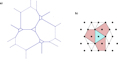
Figure 19: The web diagram (a) and toric diagram (b) for a singularity admitting a partial resolution with one $dP_{0}$ singularity (in blue) and three (symmetrically distributed) $dP_{1}$ singularities (in red).

Nevertheless, the idea is that upon partial resolution, which can be systematically analyzed, we obtain a $dP_{0}$ gauge theory, describing a visible sector, coupled in a flavour symmetric way to three $dP_{1}$ supersymmetry breaking sectors. Choosing the dynamical scale of the latter gauge sectors equal (in line with the symmetry we try to preserve), the soft terms induced in the $dP_{0}$ sector arise symmetrically for the three families .

4.2 ${\bf\Delta_{27}}$ models

Although we have focused on toric geometries, it should be clear that the main idea of using local CY geometries with several D-brane sectors is more general. A simple generalization would be to consider non-toric geometries, for instance local CY geometries containing a non-abelian orbifold singularity. In fact, this kind of generalization has an immediate application, since D-branes at the non-abelian orbifold singularity $\bf C^{3}/\Delta_{27}$ have been suggested to lead to semirealistic visible sectors [33, 34, 35].

In fact, we can use our tools to construct e.g. a local CY geometry with one sector of D3-branes at a ${\bf\Delta_{27}}$ singularity, and a supersymmetry breaking sector of D-branes at a $dP_{1}$ singularity. The $\bf C^{3}/\Delta_{27}$ singularity is obtained by modding out $\bf C^{3}$ (parametrized by complex coordinates $z_{1},z_{2},z_{3}$) by the actions

$$\theta : (z_{1},z_{2},z_{3})\to(\alpha z_{1},\alpha^{-1}z_{2},z_{3})$$

$$\omega : (z_{1},z_{2},z_{3})\to(z_{1},\alpha z_{2},\alpha^{-1}z_{3})$$

$$\sigma : (z_{1},z_{2},z_{3})\to(z_{2},z_{3},z_{1})$$ (4.2)

with $\alpha=e^{2\pi i/3}$.

The quotient by the subgroup generated by $\theta$, $\omega$ defines a $\bf C^{3}/(\bf Z_{3}\times\bf Z_{3})$ geometry, which is a toric geometry. Hence $\bf C^{3}/\Delta_{27}$ can be regarded as a quotient of this geometry by the $\bf Z_{3}$ action generated by $\sigma$, which cyclically permutes the three complex planes. Similarly, a geometry containing a ${\bf\Delta_{27}}$ singularity and e.g. a $dP_{1}$ singularity can be regarded as a $\bf Z_{3}$ quotient of a geometry containing a $\bf C^{3}/(\bf Z_{3}\times\bf Z_{3})$ singularity and three $dP_{1}$ singularities with a distribution invariant under cyclic permutation of the complex coordinates.

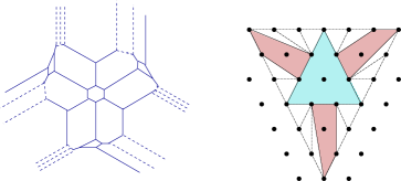
Figure 20: The parent toric geometry for the $\bf C^{3}/\Delta_{27}$ singularity with a supersymmetry breaking sector (given by $dP_{1}$) coupling in an universal way to the visible sector.

The construction of these ‘parent’ geometries and the corresponding gauge theories is easy, and identical at the technical level to the previous section. Namely, we consider the web diagram of the $\bf C^{3}/(\bf Z_{3}\times\bf Z_{3})$ singularity, and add the web diagrams of three $dP_{1}$ singularities in a way that preserves the $\bf Z_{3}$ symmetry of the diagram. The web and toric diagrams of a possible complete geometry are shown in Figure 20. Despite the complicated appearance of the diagram, it is closely related to a $\bf C^{3}/(\bf Z_{6}\times\bf Z_{6})$ singularity, so it is tractable in principle. Notice however the different spirit of the construction as compared to previous section, in that here we are ultimately interested in quotienting by the permutation symmetry among the complex planes, in order to generate the ${\bf\Delta_{27}}$ singularity. Once a parent geometry is constructed, and the gauge theory identified, the quotient gauge theory can be obtained by using techniques in [54].

We hope this example suffices to illustrate the use of our ideas in somewhat more general contexts.

4.3 Complex deformed CY’s with several singularities

In this paper we have described the construction of configurations of D-branes at different singularities in a local CY geometry, obtained by partial resolution. This has the advantage of allowing for a simple computation of the messenger sector. On the other hand, it requires an additional discussion of the stabilization of distance between singularities (via some mechanism of Kahler moduli stabilization, whose description is not completely clear in the local model).

We would like to briefly mention an alternative proposal, based on CY geometries where the structure of singularities arises after complex deformation. As in the previous situation, the construction of a geometry containing e.g. two isolated singularities of the desired kind can be systematically carried out, by combining the corresponding web diagrams. Specifically, a toric singularity admits a complex deformation to a geometry with two daughter singularities if the external legs of the web diagram of the parent singularity can be separated in two subsets, corresponding to the external legs of the web diagrams of the daughter singularities. This criterion, used in [58, 18] in the physical context, dovetails the mathematical description in [59, 60, 61].

The complex deformation setup has the advantage that the modulus controlling the distance between the singularities is a complex structure modulus, which can be stabilized using 3-form fluxes. One may interpret this as a source of UV sensitivity. However, the complex structure deformation can be entirely described in terms of the gauge theory of the initial singularity, as the confining gauge dynamics of a set of fractional D-branes (the so-called deformation branes), in analogy with [17, 18]. Efficient tools to carry out this gauge theory analysis, and hence determine the effect of complex deformation on the D-brane sectors, have been introduced in [32]. From the viewpoint of the gauge theory, the distance between the final D-brane stacks is related to the strong dynamics scale of the deformation fractional branes, clearly showing that it is not a modulus of the configuration (more precisely, it still has a dependence on the string coupling, which is nevertheless not a local modulus, hence its stabilized value depends on the global structure). In fact, it is this gauge theory description, rather than the geometric one, which is reliable in the regime of interest where the distance between the singularities is smaller than the string scale.

Hence one can in principle describe the complete dynamics in terms of the gauge theory associated to D-branes at the singularity obtained by shrinking all cycles in the geometry. This is similar to what happened in the partial resolution setup. However, the splitting of this initial singularity into several is a strong coupling effect triggered by confinement of the deformation fractional branes. The low-energy dynamics after this confinement can be determined reliably, and leads to two decoupled sectors corresponding to D3-branes at the two daughter singularities. On the other hand, the messenger sector corresponds to the massive states of the confining theory (with mass determined by the strong dynamics scale, or the complex deformation parameter in geometric terms) and cannot be reliably computed.

Since this setup lacks the computability of the partial resolution setup, we prefer to skip its detailed discussion, and simply mention one example of a singularity admitting a complex deformation to a geometry with a $dP_{0}$ and a $dP_{1}$ singularity. The relevant web diagram and toric diagrams are shown in Figure 21. The model building application of such configurations are very similar to those described in the partial resolution setup. The relevant gauge theory analysis to obtain the final two decoupled gauge theory sectors from the gauge theory of D3-branes at the parent singularity are provided in [32], to which we refer the interested reader.

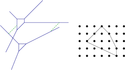
Figure 21: Web diagram and toric diagram of a singularity admitting a complex deformation to a geometry with a $dP_{0}$ and a $dP_{1}$ singularities. For clarity we have shown the web diagram explicitly split in two sub-webs, namely after the complex deformation. The finite size 3-cycle is shown as a dashed green segment.

5 Final comments

In this paper we have exploited tools to construct systems of D3-branes at CY geometries with several singularities in order to embed models of GMSB in string theory. The construction is simple and flexible and allows many generalizations. It would be interesting to develop tools to study the effects of supersymmetry breaking both on the visible sector, and on the geometry itself. In this latter respect, it would be interesting to determine the effects of supersymmetry breaking on the Kahler moduli which control the distance between the brane stacks (and which we have assumed to be stabilized at a high scale).

Notice that although very interesting, models of D3-branes at singularities are not the only possible realization of GMSB in local models. For instance, it would be interesting to develop local models where the D-branes in the visible and DSB sector are not necessarily of the same kind (parallel D3-branes in our case). One can e.g. imagine a local geometry with two sets of intersecting D-branes leading to two chiral sectors decoupled at the level of massless states. Such models would perhaps be more generic and rich, but simple problems in our setup, like the determination of the messenger sector, are probably difficult in these other situations.

We leave these and other issues as interesting open questions for the future.

Acknowledgements

We thank S. Franco, L. E. Ibáñez for useful conversations . F.S. and I.G.-E. thank CERN TH for hospitality during completion of this project. A.M.U. thanks Tel Aviv University for hospitality, and M. González for kind encouragement and support. This work has been partially supported by CICYT (Spain) under project FPA-2003-02877, and the RTN networks MRTN-CT-2004-503369 ‘The Quest for Unification: Theory confronts Experiment’, and MRTN-CT-2004-005104 ‘Constituents, Fundamental Forces and Symmetries of the Universe’. The research of F.S. is supported by the Ministerio de Educación y Ciencia through an F.P.U grant. The research of I.G.-E. is supported by the Gobierno Vasco PhD fellowship program and the Marie Curie EST program.

Appendix A Massive sector in partial resolutions

In this appendix we provide the derivation of the spectrum of states becoming massive in the partial resolution of a singularity into two. The derivation is based on the description in [32], and can in fact be considered an additional appendix to that reference.

In a partial resolution, the dimer diagram leads to two daughter dimer diagrams. Denote F, E, V and F_i, E_i, V_i, $i=1,2$ the number of faces, edges and vertices in the initial and daughter diagrams. Recall they satisfy the Euler formulas $F-E+V=0$, $F_{i}-E_{i}+V_{i}=0$. Also, each daughter dimer diagram has the same vertices as the initial one, hence $V_{i}=V$. Finally, we denote $N_{i}$ the number of D3-branes at the $i^{th}$ daughter singularity, and $N=N_{1}+N_{2}$ the initial number.

The number of gauge bosons becoming massive in the Higgs mechanism associated to the partial resolution (namely $U(N)^{F}\rightarrow U(N_{1})^{F_{1}}\times U(N_{2})^{F_{2}}$) is

$$n_{V}\,=\,F(N_{1}+N_{2})^{2}-F_{1}(N_{1})^{2}-F_{2}(N_{2})^{2}=(F-F_{1})N_{1}^{2}+(F-F_{2})N_{2}^{2}+2FN_{1}N_{2}$$ (A.1)

Also, the number of chiral multiplets which become massive is

$$n_{ch}\,=\,E(N_{1}+N_{2})^{2}-E_{1}(N_{1})^{2}-E_{2}(N_{2})^{2}=(E-E_{1})N_{1}^{2}+(E-E_{2})N_{2}^{2}+2EN_{1}N_{2}$$ (A.2)

Of these latter, $n_{V}$ of them are eaten by the massless vector multiplets to lead to massive vector multiplets. Using the Euler formulas and $V_{i}=V$ we have

$$(F-F_{i})-(E-E_{i})=F-E-(F_{1}-E_{1})=0\;\rightarrow\;F-F_{i}=E-E_{i}$$ (A.3)

Hence $(E-E_{i})N_{i}^{2}$ chiral multiplets are eaten by the $(F-F_{i})N_{i}^{2}$ vector multiplets, and similarly $2FN_{1}N_{2}$ chiral multiplets out of the $2FN_{1}N_{2}$ are eaten by the corresponding vector multiplets. The remaining chiral multiplets, which are $2(E-F)N_{1}N_{2}=2VN_{1}N_{2}$ in number, pair up into massive scalar multiplets via superpotential terms as we show below.

Now, let us try to specify how all the multiplets become massive. Consider first the $(F-F_{1})N_{1}^{2}$ disappeared vector multiplets. The disappearance is due to the fact that some faces in the initial diagram recombine in the first daughter diagram. They do so because there are $(E-E_{1})$ edges which have disappeared, due to the vev of the $N_{1}\times N_{1}$ block in the corresponding bi-fundamental. This shows that the $(F-F_{1})N_{1}^{2}$ vector multiplets eat up the $(E-E_{1})N_{1}^{2}$ chiral multiplets, leading to $F-F_{1}=E-E_{1}$ massive vector multiplets in the adjoint of the $U(N_{1})$ gauge symmetry of the corresponding recombined face. Similarly for the $(F-F_{2})N_{2}^{2}$ vector and chiral multiplets. This is rule number 1 in Section 2.3.1.

In order to understand the additional $2FN_{1}N_{2}$ disappeared vector multiplets, it is useful to have a more precise picture of how the edges of a face in the initial diagram can behave. Notice that for a given face in the original dimer diagram, it is impossible that all edges are of type 3 (present in both sub-dimers). If all edges in a face would be of type 3, and given the fact that at each node there can only be two edges of type 3 (this will be proven later), then that face would correspond to a cycle on the Riemann surface wrapping the new puncture G coming from the resolution. However, since this cycle corresponds to a face in the dimer, its (p,q) charge would be zero, which is impossible. Thus every face has to have at least two edges which are not of type 3, so either two edges of the face are of type 1, i.e. disappear from sub-dimer 2, (or two are of type 2) or one edge is of type 1 and another of type 2 (see Figure 22). We denote these two cases (a) and (b)

Figure 22: Two possible configuration of edges for a face.

The $2FN_{1}N_{2}$ disappeared vector multiplets arise from open strings stretching between subdimers 1 and 2, at the same face location in both. They become massive by eating up chiral multiplets associated to open strings stretching between both sub-dimers, across disappeared edges. In case (a), the coupling occurs as shown in Figure 23.

\psfrag{a12}{$a_{12}$}\psfrag{b12}{$b_{12}$}\psfrag{A12}{$A_{12}$}\psfrag{B12}{$B_{12}$}\includegraphics[scale={0.40}]{case1_coupling.eps}

Figure 23: Coupling between chiral and vector multiplets for the case when a face has two edges of the same type.

The vector multiplets (shown as wavy arrows) $A_{12}$ and $B_{21}$ couple to the chiral multiplets $a_{12}$ and $b_{21}$ respectively (which stretch across edges $a$ and $b$ respectively). In case (b), the coupling occurs as shown in Figure 24.

\psfrag{a12}{$a_{12}$}\psfrag{b12}{$b_{12}$}\psfrag{A12}{$A_{12}$}\psfrag{B12}{$B_{12}$}\includegraphics[scale={0.40}]{case2_coupling.eps}

Figure 24: Coupling between chiral and vector multiplets for the case when a face has one edge of each type.

The vector multiplets $A_{12}$ and $B_{21}$ couple to $a_{12}$ and $b_{21}$ respectively. $a_{12}$ and $b_{21}$ stretch across edges $a$ and $b$ respectively. This can be easily generalised to a face with an arbitrary assignation of edges. The above discussion shows that for each face in the original dimer diagram, we obtain two massive vector multiplets in the bi-fundamental $(N_{1},\overline{N_{2}})$ and its conjugate, of the gauge factors at the corresponding location. This is rule number 2 in Section 2.3.1

Let us now consider the remaining $2(E-F)N_{1}N_{2}=2VN_{1}N_{2}$ chiral multiplets. As we show, they become massive due to the $V$ superpotential terms. These chiral multiplets arise from open strings stretching between the two dimer diagrams (with both orientations), across edges of type 3. The fact that each superpotential term leads to a mass for a chiral multiplet in the $(N_{1},{\overline{N_{2}}})$ and $({\overline{N_{1}}},N_{2})$ (of the faces separated by the corresponding edge) follows from the fact that each node has necessarily two edges of type 3. Namely, all fields in the superpotential term, except the two chiral multiplets, acquire vevs, leading to a mass term for the latter. Hence one recovers rule number 3 in Section 2.3.1.

The property that each node necessarily has two edges of type 3 can be shown as follows. In a partial resolution, the zig-zag paths of the original dimer diagram are split in two sets I and II. That is, the daughter dimer diagram 1 is obtained by removing the zig-zag paths II and adding the zig-zag path G which correspond to the new puncture. Similarly for dimer diagram 2, with the zigzag G being the same but with opposite orientation. Now, at each node, two edges of type 1 and 2 have to be separated by at least one edge of type 3. A little thought shows that if there are more than two edges of type 3 at any given node, the zig-zags G in both subdimers cannot be the same. This is illustrated in Figures 25 and 26. In the first Figure one sees that when only two edges of type 3 are present at a given node, then they separate the graph into two regions of type 1 and 2 respectively. Now, in the daughter dimer diagram 1 (resp. 2) all edges of type 2 (resp. 1) are absent. Hence the zigzag G of the new puncture passes through the boundary of region 1 (resp. 2), consistently leading to the same G with opposite orientation in the two diagrams. The situation for a node with more than two edges of type 3 is shown in Figure 26. Since it clearly leads to paths G which are not the same in the two dimer diagrams, we conclude that such node structure is not possible.

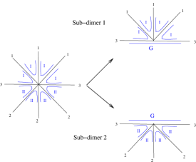
Figure 25: Resolution for the case when only two edges at a given node are of type 3. G represents the new puncture which arises in the resolution

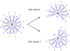
Figure 26: Resolution for the case when more than two edges at a given node are of type 3. G represents the new puncture which arises in the resolution.

One small subtlety is that for a given edge of type 3, there are actually two chiral multiplets becoming massive. These correspond to open strings stretching across this edge and going from the first daughter dimer diagram to the second and vice-versa. Each superpotential term pairs only one of these chiral multiplets (coupling it to only one of the chiral multiplets in the other adjacent type 3 node). And for a given edge of type 3, both modes acquire mass thanks to the two superpotential terms at the nodes of the edge.

References

- [1] J. Polchinski and A. Strominger, Phys. Lett. B 388 (1996) 736 [arXiv:hep-th/9510227].
- [2] K. Becker and M. Becker, Nucl. Phys. B 477 (1996) 155 [arXiv:hep-th/9605053].
- [3] K. Dasgupta, G. Rajesh and S. Sethi, JHEP 9908 (1999) 023 [arXiv:hep-th/9908088].
- [4] S. B. Giddings, S. Kachru and J. Polchinski, “Hierarchies from fluxes in string compactifications,” Phys. Rev. D 66, 106006 (2002) [arXiv:hep-th/0105097].
- [5] M. Grana, “MSSM parameters from supergravity backgrounds,” Phys. Rev. D 67, 066006 (2003) [arXiv:hep-th/0209200].
- [6] P. G. Camara, L. E. Ibanez and A. M. Uranga, “Flux-induced SUSY-breaking soft terms,” Nucl. Phys. B 689, 195 (2004) [arXiv:hep-th/0311241].
- [7] M. Grana, T. W. Grimm, H. Jockers and J. Louis, “Soft supersymmetry breaking in Calabi-Yau orientifolds with D-branes and Nucl. Phys. B 690, 21 (2004) [arXiv:hep-th/0312232].
- [8] P. G. Camara, L. E. Ibanez and A. M. Uranga, Nucl. Phys. B 708 (2005) 268 [arXiv:hep-th/0408036].
- [9] D. Lust, S. Reffert and S. Stieberger, Nucl. Phys. B 706 (2005) 3 [arXiv:hep-th/0406092].
- [10] D. Lust, S. Reffert and S. Stieberger, Nucl. Phys. B 727 (2005) 264 [arXiv:hep-th/0410074].
- [11] A. Font and L. E. Ibanez, JHEP 0503 (2005) 040 [arXiv:hep-th/0412150].
- [12] D. Lust, P. Mayr, S. Reffert and S. Stieberger, Nucl. Phys. B 732 (2006) 243 [arXiv:hep-th/0501139].
- [13] J. Gomis, F. Marchesano and D. Mateos, JHEP 0511 (2005) 021 [arXiv:hep-th/0506179].
- [14] V. S. Kaplunovsky and J. Louis, Phys. Lett. B 306 (1993) 269 [arXiv:hep-th/9303040].
- [15] A. Brignole, L. E. Ibanez and C. Munoz, Nucl. Phys. B 422 (1994) 125 [Erratum-ibid. B 436 (1995) 747] [arXiv:hep-ph/9308271].
- [16] A. Brignole, L. E. Ibanez, C. Munoz and C. Scheich, Z. Phys. C 74 (1997) 157 [arXiv:hep-ph/9508258].
- [17] I. R. Klebanov and M. J. Strassler, JHEP 0008 (2000) 052 [arXiv:hep-th/0007191].
- [18] S. Franco, A. Hanany and A. M. Uranga, “Multi-flux warped throats and cascading gauge theories,” arXiv:hep-th/0502113.
- [19] D. Berenstein, C. P. Herzog, P. Ouyang and S. Pinansky, JHEP 0509, 084 (2005) [arXiv:hep-th/0505029].
- [20] S. Franco, A. Hanany, F. Saad and A. M. Uranga, JHEP 0601, 011 (2006) [arXiv:hep-th/0505040].
- [21] M. Bertolini, F. Bigazzi and A. L. Cotrone, Phys. Rev. D 72, 061902 (2005) [arXiv:hep-th/0505055].
- [22] K. Intriligator and N. Seiberg, JHEP 0602, 031 (2006) [arXiv:hep-th/0512347].
- [23] A. Brini and D. Forcella, arXiv:hep-th/0603245.
- [24] S. Franco and A. M. .. Uranga, arXiv:hep-th/0604136.
- [25] K. Intriligator, N. Seiberg and D. Shih, arXiv:hep-th/0602239.
- [26] D. E. Diaconescu, B. Florea, S. Kachru and P. Svrcek, JHEP 0602 (2006) 020 [arXiv:hep-th/0512170].
- [27] A. Hanany and K. D. Kennaway, arXiv:hep-th/0503149.
- [28] S. Franco, A. Hanany, K. D. Kennaway, D. Vegh and B. Wecht, “Brane dimers and quiver gauge theories,” arXiv:hep-th/0504110.
- [29] A. Hanany and D. Vegh, arXiv:hep-th/0511063.
- [30] B. Feng, Y. H. He, K. D. Kennaway and C. Vafa, arXiv:hep-th/0511287.
- [31] S. Franco and D. Vegh, arXiv:hep-th/0601063.
- [32] I. Garcia-Etxebarria, F. Saad and A. M. Uranga, arXiv:hep-th/0603108.
- [33] G. Aldazabal, L. E. Ibanez, F. Quevedo and A. M. Uranga, JHEP 0008 (2000) 002 [arXiv:hep-th/0005067].
- [34] D. Berenstein, V. Jejjala and R. G. Leigh, Phys. Rev. Lett. 88 (2002) 071602 [arXiv:hep-ph/0105042].
- [35] H. Verlinde and M. Wijnholt, arXiv:hep-th/0508089.
- [36] I. R. Klebanov and E. Witten, singularity,” Nucl. Phys. B 536 (1998) 199 [arXiv:hep-th/9807080].
- [37] M. Bertolini, F. Bigazzi and A. L. Cotrone, JHEP 0412 (2004) 024 [arXiv:hep-th/0411249].
- [38] S. Benvenuti, S. Franco, A. Hanany, D. Martelli and J. Sparks, JHEP 0506 (2005) 064 [arXiv:hep-th/0411264].
- [39] S. Benvenuti and M. Kruczenski, L(p,qr),” arXiv:hep-th/0505206.
- [40] S. Franco, A. Hanany, D. Martelli, J. Sparks, D. Vegh and B. Wecht, JHEP 0601 (2006) 128 [arXiv:hep-th/0505211].
- [41] A. Butti, D. Forcella and A. Zaffaroni, JHEP 0509 (2005) 018 [arXiv:hep-th/0505220].
- [42] A. Butti and A. Zaffaroni, JHEP 0511 (2005) 019 [arXiv:hep-th/0506232].
- [43] S. Franco, Y. H. He, C. Herzog and J. Walcher, Phys. Rev. D 70 (2004) 046006 [arXiv:hep-th/0402120].
- [44] C. P. Herzog, Q. J. Ejaz and I. R. Klebanov, JHEP 0502 (2005) 009 [arXiv:hep-th/0412193].
- [45] O. Aharony and A. Hanany, Nucl. Phys. B 504, 239 (1997) [arXiv:hep-th/9704170].
- [46] O. Aharony, A. Hanany and B. Kol, JHEP 9801, 002 (1998) [arXiv:hep-th/9710116].
- [47] N. C. Leung and C. Vafa, Adv. Theor. Math. Phys. 2, 91 (1998) [arXiv:hep-th/9711013].
- [48] R. G. Leigh and M. Rozali, Phys. Rev. D 59 (1999) 026004 [arXiv:hep-th/9807082].
- [49] G. Aldazabal, D. Badagnani, L. E. Ibanez and A. M. Uranga, JHEP 9906 (1999) 031 [arXiv:hep-th/9904071].
- [50] M. Bianchi and J. F. Morales, arXiv:hep-th/0101104.
- [51] L. E. Ibanez, R. Rabadan and A. M. Uranga, Nucl. Phys. B 542 (1999) 112 [arXiv:hep-th/9808139].
- [52] D. R. Morrison and M. R. Plesser, Adv. Theor. Math. Phys. 3 (1999) 1 [arXiv:hep-th/9810201].
- [53] S. Elitzur, A. Giveon and D. Kutasov, Phys. Lett. B 400 (1997) 269 [arXiv:hep-th/9702014].
- [54] A. M. Uranga, JHEP 9901 (1999) 022 [arXiv:hep-th/9811004].
- [55] M. Aganagic, A. Karch, D. Lust and A. Miemiec, Nucl. Phys. B 569 (2000) 277 [arXiv:hep-th/9903093].
- [56] S. Willenbrock, Phys. Lett. B 561 (2003) 130 [arXiv:hep-ph/0302168].
- [57] A. Hanany, P. Kazakopoulos and B. Wecht, JHEP 0508 (2005) 054 [arXiv:hep-th/0503177].
- [58] M. Aganagic and C. Vafa, arXiv:hep-th/0110171.
- [59] K. Altmann, ‘The versal Deformation of an isolated toric Gorenstein Singularity’, alg-geom/9403004.
- [60] K. Altmann, ‘Infinitesimal Deformations and Obstructions for Toric Singularities’, alg-geom/9405008.
- [61] K. Altmann, ‘Deformations of toric singularities’, Habilitationsschrift; Humboldt-Universitt zu Berlin 1995, available at http://page.mi.fu-berlin.de/ altmann/PAPER/