OU-HET 560 May 2006

${\cal N}=4$ SYM on $R\times S^{3}$ and Theories with 16 Supercharges

Goro Ishiki, Yastoshi Takayama and Asato Tsuchiya

Department of Physics, Graduate School of Science
Osaka University, Toyonaka, Osaka 560-0043, Japan

We study ${\cal N}=4$ SYM on $R\times S^{3}$ and theories with 16 supercharges arising as its consistent truncations. These theories include the plane wave matrix model, ${\cal N}=4$ SYM on $R\times S^{2}$ and ${\cal N}=4$ SYM on $R\times S^{3}/Z_{k}$, and their gravity duals were studied by Lin and Maldacena. We make a harmonic expansion of the original ${\cal N}=4$ SYM on $R\times S^{3}$ and obtain each of the truncated theories by keeping a part of the Kaluza-Klein modes. This enables us to analyze all the theories in a unified way. We explicitly construct some nontrivial vacua of ${\cal N}=4$ SYM on $R\times S^{2}$. We perform 1-loop analysis of the original and truncated theories. In particular, we examine states regarded as the integrable $SO(6)$ spin chain and a time-dependent BPS solution, which is considered to correspond to the AdS giant graviton in the original theory.

1 Introduction

It is important to collect various examples of the gauge/gravity correspondence in order to elucidate how universal this phenomena is. Recently this direction has been pursued successfully by Lin and Maldacena [1]. They gave a general method for constructing the gravity solutions dual to a family of theories with 16 supercharges. All these theories share the common feature that they have a mass gap, a discrete spectrum of excitations and a dimensionless parameter, which connect weak and strong coupling regions. This method is an extension of the so-called bubbling AdS geometries [2, 4, 3]. The symmetry algebra of some of the theories is $SU(2|4)$ supergroup, while the other theories have $SO(4)\times SO(4)$ symmetry. The theories with the $SU(2|4)$ symmetry arise as consistent truncations of ${\cal N}=4$ super Yang Mills (SYM) on $R\times S^{3}$ as explained below. They include the plane wave matrix model [5], ${\cal N}=4$ SYM on $R\times S^{2}$ [6] and ${\cal N}=4$ SYM on $R\times S^{3}/Z_{k}$.

${\cal N}=4$ SYM on $R\times S^{3}$ has the superconformal symmetry $SU(2,2|4)$, whose bosonic subgroup is $SO(2,4)\times SO(6)$, where $SO(2,4)$ is the conformal group in 4 dimensions and $SO(6)$ is the R-symmetry. $SO(2,4)$ has a subgroup $SO(4)$ that is the isometry of the $S^{3}$ on which the theory is defined. $SO(4)$ is identified with $SU(2)\times\tilde{SU}(2)$, where we marked one of two $SU(2)$’s with a tilde to focus on it. By quotienting the original ${\cal N}=4$ SYM on $R\times S^{3}$ by various subgroups of $\tilde{SU}(2)$, one obtains the above mentioned theories whose symmetry algebra is $SU(2|4)$. Quotienting by full $\tilde{SU}(2)$, $U(1)$ and $Z_{k}$ give rise to the plane wave matrix model, ${\cal N}=4$ SYM on $R\times S^{2}$ and ${\cal N}=4$ SYM on $R\times S^{3}/Z_{k}$, respectively. Indeed, the consistent truncation to the plane wave matrix model was first found in [10]. The original ${\cal N}=4$ SYM on $R\times S^{3}$ has a unique vacuum, while the truncated theories have many vacua. The method by Lin and Maldacena give in principle gravity solutions that describe these vacua and fluctuations around them, and they indeed obtained a few explicit solutions [1].

It is obviously relevant to study the dynamics of the above truncated theories and compare the results with those obtained on the gravity side. Indeed, some studies on the dynamics of the plane wave matrix model have already been carried out [6]$\sim$[13]. It should also be worthwhile to study the original ${\cal N}=4$ SYM on $R\times S^{3}$ itself [14]$\sim$[17], although it is believed to be equivalent to ${\cal N}=4$ SYM on $R^{4}$ at conformal point, which is much easier to analyze. The reasons are as follows. First, the pp-wave limit on the gravity side is taken for $AdS_{5}\times S^{5}$ in the global coordinates, and the boundary of $AdS_{5}$ is $R\times S^{3}$. The holography in the pp-wave limit could, therefore, be well understood in ${\cal N}=4$ SYM on $R\times S^{3}$. Next, the original theory has a classical time-dependent BPS solution, which is considered to correspond to the AdS giant graviton [18, 3]. The quantum dynamics of the AdS giant graviton is expected to be understood by examining the quantum fluctuation around this classical solution. The classical solution is, however, mapped to a classical vacuum solution of ${\cal N}=4$ SYM on $R^{4}$ that breaks the conformal symmetry, so that the equivalence between ${\cal N}=4$ SYM on $R\times S^{3}$ and $R^{4}$ does not seem to hold in this case. Third, one can consider ${\cal N}=4$ SYM on $S^{1}\times S^{3}$, which is the finite temperature version of ${\cal N}=4$ SYM on $R\times S^{3}$ and is not equivalent to ${\cal N}=4$ SYM on $R^{4}$. This theory is known to show a phase transition [19, 20, 21], which should correspond to the thermal phase transition between the AdS space and the AdS black hole [22]. The study of ${\cal N}=4$ SYM on $R\times S^{3}$ serves as a preparation for that of this theory.

In this paper, we study the dynamics of the original ${\cal N}=4$ SYM on $R\times S^{3}$ and the truncated theories, by making a harmonic expansion of the original theory on $S^{3}$. We obtain each of the truncated theories by keeping a part of the Kaluza-Klein (KK) modes of the original theory. This enables us to analyze all of the original and truncated theories in a unified way.

In section 2, we review basic properties of ${\cal N}=4$ SYM on $R\times S^{3}$. In section 3, we develop the harmonic expansion on $S^{3}$. In particular, we obtain a new formula for the integral of the product of three harmonics, which is used in the following sections. In section 4, by applying the results of section 3, we carry out a harmonic expansion of ${\cal N}=4$ SYM on $R\times S^{3}$ including all interaction terms. The result in this section is an extension of the work[10], where the authors carried out the mode expansion of the free part in detail and analyzed interactions between the lowest modes needed for the truncation to the plane wave matrix model.

In section 5, we describe the consistent truncations of the original ${\cal N}=4$ SYM on $R\times S^{3}$ to the theories with $SU(2|4)$ symmetry. We realize each quotienting by keeping a part of the KK modes of the original theory. We verify that quotienting by $U(1)$ indeed yields ${\cal N}=4$ SYM on $R\times S^{2}$ by comparing the KK modes we kept with the KK modes of ${\cal N}=4$ SYM on $R\times S^{2}$. We explicitly construct some of the nontrivial vacua of ${\cal N}=4$ SYM on $R\times S^{2}$ in terms of the KK modes.

In section 6, we first calculate 1-loop diagrams in the original theory. We introduce cut-offs for loop angular momenta and see that this cut-off scheme yield correct coefficients of logarithmic divergences, which are consistent with the Ward identities and the vanishing of the beta function. We next determine some counter terms in the original theory and the truncated theories in the trivial vacuum by using the non-renormalization of energy of the BPS states. This reveals that the states built by the sequence of the scalars in both the original theory and the truncated theories in the trivial vacuum are mapped to the same integrable $SO(6)$ spin chain.

In section 7, we examine the time-independent BPS solution in the original and truncated theories, which is considered to correspond to the AdS giant graviton in the original theory. We see that the 1-loop effective action around this solution vanishes.

Section 8 is devoted to summary and discussion. In appendix A, we gather some formulae concerning the representation of $SU(2)$. In appendix B, we describe the vertex coefficients which are used in representing the interaction terms by the modes. In appendix C, we describe some properties of the spherical harmonics on $S^{2}$, which are used in section 5. In appendix D, we list the 1-loop diagrams and the divergent parts of those diagrams. In appendix E, we give the expressions for the 1-loop effective action around the time dependent BPS solution in the truncated theories.

2 Basic properties of ${\cal N}=4$ SYM on $R\times S^{3}$

In this section, we review the basic properties of ${\cal N}=4$ SYM on $R\times S^{3}$ [14]$\sim$[17]. We restrict ourselves to the $U(N)$ gauge group and the ’t Hooft limit throughout this paper. However, the generalization to other gauge groups that allow the ’t Hooft limit is easy. We follow the notation of [17] with slight modification. We set the radius of $S^{3}$ at one. Borrowing the ten-dimensional notation, we can write down the action as follows:

$$S=\frac{1}{g_{YM}^{2}}\int d^{4}x\>e\>\mbox{Tr}\left(-\frac{1}{4}F_{ab}F^{ab}-\frac{1}{2}D_{a}X_{m}D^{a}X_{m}-\frac{1}{12}RX_{m}^{2}\right.$$

$$\hskip 113.81102pt\left.-\frac{i}{2}\bar{\lambda}\Gamma^{a}D_{a}\lambda-\frac{1}{2}\bar{\lambda}\Gamma^{m}[X_{m},\lambda]+\frac{1}{4}[X_{m},X_{n}]^{2}\right),$$ (2.1)

where $a$ and $b$ are local Lorentz indices and run from $0$ to $3$, and $m$ runs from $4$ to $9$. $\Gamma^{a}$ and $\Gamma^{m}$ are the 10-dimensional gamma matrices, which satisfy

$$\{\Gamma^{a},\Gamma^{b}\}=2\eta^{ab},\;\;\;\;\;\{\Gamma^{m},\Gamma^{n}\}=2\delta^{mn},$$ (2.2)

where $\eta^{ab}=\mbox{diag}(-1,1,1,1)$. $\lambda$ is the Majorana-Weyl spinor in 10 dimensions. $e$ is the determinant of the vierbein $e_{\mu}^{a}$ on $R\times S^{3}$. $R$ is the scalar curvature of $S^{3}$ which is equal to $6$. The field strength and the covariant derivatives take the form

$$F_{ab}=\nabla_{a}A_{b}-\nabla_{b}A_{a}-i[A_{a},A_{b}]=e_{a}^{\mu}e_{b}^{\nu}F_{\mu\nu},$$

$$D_{a}X_{m}=\nabla_{a}X_{m}-i[A_{a},X_{m}],$$

$$D_{a}\lambda=\nabla_{a}\lambda-i[A_{a},\lambda],$$ (2.3)

where

$$\nabla_{a}A_{b}=e^{\mu}_{a}(\partial_{\mu}A_{b}+\omega_{\mu b}^{\;\;\;\;\;c}A_{c}),\;\;\;\nabla_{a}X_{m}=e^{\mu}_{a}\partial_{\mu}X_{m},\;\;\;\nabla_{a}\lambda=e^{\mu}_{a}(\partial_{\mu}\lambda+\frac{1}{4}\omega_{\mu}^{bc}\Gamma_{bc}\lambda),$$ (2.4)

and $\omega_{\mu}^{ab}$ is the spin connection on $R\times S^{3}$ determined by $de^{a}+\omega^{a}_{\;b}\wedge e^{b}=0$.

The classical action (2.1) with arbitrary gauge group has the superconformal symmetry $SU(2,2|4)$. This symmetry is preserved at the quantum level. This is ensured by the following two facts. One is that the Weyl anomaly for the $g_{YM}=0$ was shown to vanish on $R\times S^{3}$ [23]. The other is that the beta function vanishes for arbitrary $g_{YM}$ because it only reflects the short distance structure of the theory and indeed vanishes on $R^{4}$. In what follows, we describe the transformation laws of the fields under each element of $SU(2,2|4)$ and see that the action (2.1) is invariant under such transformations.

First, let us see the conformal invariance of the action. If the metric and the vierbein were allowed to vary, the action would possess the Weyl invariance,

$$\delta_{W}A_{a}=-\alpha A_{a},\;\;\;\delta_{W}X_{m}=-\alpha X_{m},\;\;\;\delta_{W}\lambda=-\frac{3}{2}\alpha\lambda,\;\;\;\delta_{W}e_{\mu}^{a}=\alpha e_{\mu}^{a},$$ (2.5)

the diffeomorphism invariance,

$$\delta_{\xi}A_{a}=\xi^{\mu}\partial_{\mu}A_{a},\;\;\;\delta_{\xi}X_{m}=\xi^{\mu}\partial_{\mu}X_{m},\;\;\;\delta_{\xi}\lambda=\xi^{\mu}\partial_{\mu}\lambda,$$

$$\delta_{\xi}e_{\mu}^{a}=\xi^{\nu}\nabla_{\nu}e_{\mu}^{a}+\nabla_{\mu}\xi^{\nu}e_{\nu}^{a}.$$ (2.6)

and the local Lorentz invariance,

$$\delta_{L}A_{a}=\varepsilon_{a}^{\;b}A_{b},\;\;\;\delta_{L}X_{m}=0,\;\;\;\delta_{L}\lambda=\frac{1}{4}\varepsilon_{ab}\Gamma^{ab}\lambda,\;\;\;\delta_{L}e_{\mu}^{a}=\varepsilon^{a}_{\;b}e_{\mu}^{b}.$$ (2.7)

Let $\xi$ be a conformal Killing vector satisfying

$$\nabla_{a}\xi_{b}+\nabla_{b}\xi_{a}=\frac{1}{2}\nabla_{c}\xi^{c}\eta_{ab},$$ (2.8)

and set $\alpha=-\frac{1}{4}\nabla_{a}\xi^{a}$ and $\varepsilon_{ab}=\xi^{\mu}\omega_{\mu ab}+\frac{1}{2}(\nabla_{a}\xi_{b}-\nabla_{b}\xi_{a})$. Then,

$$(\delta_{\xi}+\delta_{W}+\delta_{L})e_{\mu}^{a}=0.$$ (2.9)

The action is, therefore, invariant under the conformal transformation $\delta_{c}=\delta_{\xi}+\delta_{W}+\delta_{L}$, where the metric and the vierbein are fixed. The conformal transformation act on each field as follows:

$$\delta_{c}A_{a}=\xi^{b}\nabla_{b}A_{a}+\nabla_{a}\xi^{b}A_{b},$$

$$\delta_{c}X_{m}=\xi^{a}\nabla_{a}X_{m}+\frac{1}{4}\nabla_{a}\xi^{a}X_{m},$$

$$\delta_{c}\lambda=\xi^{a}\nabla_{a}\lambda+\frac{1}{4}\nabla_{a}\xi_{b}\Gamma^{ab}\lambda+\frac{3}{8}\nabla_{a}\xi^{a}\lambda.$$ (2.10)

It is often convenient to rewrite the action in the the $SU(4)$ symmetric form. The 10-dimensional Lorentz group has been decomposed as $SO(9,1)\supset SO(3,1)\times SO(6)$. We identify $SO(6)$ with $SU(4)$. We use $A,B=1,2,3,4$ as the indices of $4$ in $SU(4)$ while we have used $m,n=4,\cdots,9$ as the indices of $6$ in $SO(6)$. The $SO(6)$ vector, $6$, corresponds to the antisymmetric tensor of $4$ in $SU(4)$. The $SO(6)$ and $SU(4)$ basis are related as

$$X_{i4}=\frac{1}{2}(X_{i+3}+iX_{i+6})\;\;\;(i=1,2,3),$$

$$X_{AB}=-X_{BA},\;\;\;X^{AB}=-X^{BA}=X_{AB}^{\dagger},\;\;\;X^{AB}=\frac{1}{2}\epsilon^{ABCD}X_{CD},$$ (2.11)

Similar identities hold for the gamma matrices:

$$\Gamma^{i4}=\frac{1}{2}(\Gamma^{i+3}-i\Gamma^{i+6}),\;\;\;\mbox{etc.}$$ (2.12)

The 10-dimensional gamma matrices are decomposed as

$$\Gamma^{a}=\gamma^{a}\otimes 1_{8},\;\;\;\Gamma^{AB}=\gamma_{5}\otimes\left(\begin{array}[]{cc}0&-\tilde{\rho}^{AB}\\ \rho^{AB}&0\end{array}\right)=-\Gamma^{BA},$$ (2.15)

where $\gamma^{a}$ is the 4-dimensional gamma matrix, satisfying $\{\gamma^{a},\gamma^{b}\}=2\eta^{ab}$, and $\gamma_{5}=i\gamma^{0}\gamma^{1}\gamma^{2}\gamma^{3}$. $\Gamma^{AB}$ satisfies $\{\Gamma^{AB},\Gamma^{CD}\}=\epsilon^{ABCD}$, and $\rho^{AB}$ and $\tilde{\rho}^{AB}$ are defined by

$$(\rho^{AB})_{CD}=\delta^{A}_{C}\delta^{B}_{D}-\delta^{A}_{D}\delta^{B}_{C},\;\;\;(\tilde{\rho}^{AB})^{CD}=\epsilon^{ABCD}.$$ (2.16)

The charge conjugation matrix and the chirality matrix are given by

$$C_{10}=C_{4}\otimes\left(\begin{array}[]{cc}0&1_{4}\\ 1_{4}&0\end{array}\right),\;\;\;\;\;\Gamma^{11}=\Gamma^{0}\cdots\Gamma^{9}=\gamma_{5}\otimes\left(\begin{array}[]{cc}1_{4}&0\\ 0&-1_{4}\end{array}\right),$$ (2.21)

where $(\Gamma^{a,m})^{T}=-C_{10}^{-1}\Gamma^{a,m}C_{10}$ and $C_{4}$ is the charge conjugation matrix in 4 dimensions. The Majorana-Weyl spinor in 10 dimensions is decomposed as

$$\lambda=\Gamma_{11}\lambda=\left(\begin{array}[]{c}\lambda_{+}^{A}\\ \lambda_{-A}\end{array}\right),$$ (2.24)

where $\lambda_{-A}$ is the charge conjugation of $\lambda_{+}^{A}$:

$$\lambda_{-A}=(\lambda_{+}^{A})^{c}=C_{4}(\bar{\lambda}_{+A})^{T},\;\;\;\;\;\gamma_{5}\lambda_{\pm}=\pm\lambda_{\pm}.$$ (2.25)

The action is rewritten in terms of $SU(4)$ symmetric notation as follows:

$$S=\frac{1}{g_{YM}^{2}}\int d^{4}x\>e\>\mbox{Tr}\left(-\frac{1}{4}F_{ab}F^{ab}-\frac{1}{2}D_{a}X_{AB}D^{a}X^{AB}-\frac{1}{2}X_{AB}X^{AB}-i\bar{\lambda}_{+A}\gamma^{a}D_{a}\lambda_{+}^{A}\right.$$

$$\hskip 113.81102pt\left.-\bar{\lambda}_{+A}[X^{AB},\lambda_{-B}]-\bar{\lambda}_{-}^{A}[X_{AB},\lambda_{+}^{B}]+\frac{1}{4}[X_{AB},X_{CD}][X^{AB},X^{CD}]\right),$$

(2.26)

It is easy to see that the action (2.26) is invariant under the $SU(4)$ R-symmetry

$$\delta_{R}X^{AB}=iT^{A}_{\;\;C}X^{CB}+iT^{B}_{\;\;C}X^{AC},\;\;\;\delta_{R}\lambda_{+}^{A}=iT^{A}_{\;\;B}\lambda_{+}^{B},\;\;\;\delta_{R}\bar{\lambda}_{-A}=-i\bar{\lambda}_{-B}T^{B}_{\;\;A},$$ (2.27)

where $T^{A}_{\;\;B}$ is a hermitian traceless matrix.

Finally, we consider the superconformal symmetry. The conformal Killing spinor equation on $R\times S^{3}$ takes the form

$$\nabla_{a}\epsilon_{+}=\pm\frac{i}{2}\gamma_{a}\gamma^{0}\epsilon_{+},\;\;\;\;\;\gamma_{5}\epsilon_{+}=\epsilon_{+}.$$ (2.28)

A general solution to (2.28) for each sign includes arbitrary constant Weyl spinor and is obtained by projecting the Killing spinor on $AdS_{5}$ on the boundary [14, 24]. We construct a 10-dimensional Majorana-Weyl spinor as

$$\epsilon=\left(\begin{array}[]{c}\epsilon_{+}^{A}\\ \epsilon_{-A}\end{array}\right),$$ (2.31)

where $\epsilon_{+}^{A}$ satisfies (2.28) and $\epsilon_{-A}$ is the charge conjugation of $\epsilon_{+}^{A}$ and satisfies

$$\nabla_{a}\epsilon_{-A}=\mp\frac{i}{2}\gamma_{a}\gamma^{0}\epsilon_{-A},\;\;\;\;\;\gamma_{5}\epsilon_{-A}=-\epsilon_{-A}.$$ (2.32)

The action (2.1) is invariant under the superconformal transformation

$$\delta_{\epsilon}A_{a}=i\bar{\lambda}\Gamma_{a}\epsilon,\;\;\;\delta_{\epsilon}X_{m}=i\bar{\lambda}\Gamma_{m}\epsilon,$$

$$\delta_{\epsilon}\lambda=\left[\frac{1}{2}F_{ab}\Gamma^{ab}+D_{a}X_{m}\Gamma^{a}\Gamma^{m}-\frac{1}{2}X_{m}\Gamma^{m}\Gamma^{a}\nabla_{a}-\frac{i}{2}[X_{m},X_{n}]\Gamma^{mn}\right]\epsilon.$$ (2.33)

$\epsilon_{+}$ in (2.28) includes four real degrees of freedom for each sign as mentioned above and there are four $SU(4)$ indices, so that $\epsilon$ in (2.31) possess 32 real degrees of freedom. Namely, the superconformal symmetry (2.33) has 32 real supercharges. In the $SU(4)$ symmetric notation, the transformation (2.33) is written as

$$\delta_{\epsilon}A_{a}=i(\bar{\lambda}_{+A}\gamma_{a}\epsilon_{+}^{A}-\bar{\epsilon}_{+A}\gamma_{a}\lambda_{+}^{A}),$$

$$\delta_{\epsilon}X^{AB}=i(-\bar{\epsilon}_{-}^{A}\lambda_{+}^{B}+\bar{\epsilon}_{-}^{B}\lambda_{+}^{A}+\epsilon^{ABCD}\bar{\lambda}_{+C}\epsilon_{-D}),$$

$$\delta_{\epsilon}\lambda_{+}^{A}=\frac{1}{2}F_{ab}\gamma^{ab}\epsilon_{+}^{A}+2D_{a}X^{AB}\gamma^{a}\epsilon_{-B}+X^{AB}\gamma^{a}\nabla_{a}\epsilon_{-B}+2i[X^{AC},X_{CB}]\epsilon_{+}^{B},$$

$$\delta_{\epsilon}\lambda_{-A}=\frac{1}{2}F_{ab}\gamma^{ab}\epsilon_{-A}+2D_{a}X_{AB}\gamma^{a}\epsilon_{+}^{B}+X_{AB}\gamma^{a}\nabla_{a}\epsilon_{+}^{B}+2i[X_{AC},X^{CB}]\epsilon_{-B}.$$ (2.34)

In the remaining of this section, we make a comment on the equivalence between ${\cal N}=4$ SYM on $R^{4}$ at conformal point and ${\cal N}=4$ SYM on $R\times S^{3}$. We first see the relationship between $R^{4}$ and $R\times S^{3}$. If one starts with the metric of $R^{4}$,

$$ds^{2}=dr^{2}+r^{2}d\Omega_{3}^{2},$$ (2.35)

makes a change of variable, $\ln r=\tau$, and defines a new metric through a Weyl transformation, $ds^{2}=e^{2\tau}{ds^{\prime}}^{2}$, one obtains the metric of euclidean $R\times S^{3}$,

$${ds^{\prime}}^{2}=d\tau^{2}+d\Omega_{3}^{2}.$$ (2.36)

The analytical continuation, $\tau=it$, yields the metric of $R\times S^{3}$. This indicates how these two theories are related. There is one to one correspondence between operators on $R^{4}$ and states on $R\times S^{3}$ as common in conformal fields theories. Namely, one can move an operator at arbitrary point on $R^{4}$ to the origin by a conformal transformation, and map it to an state on $R\times S^{3}$ because $r\rightarrow 0$ corresponds to $t\rightarrow-\infty$. One can also see from $\ln r=\tau$ that the dilatation operator on $R^{4}$ corresponds to hamiltonian on $R\times S^{3}$. That is, the scaling dimension $\Delta$ on $R^{4}$ corresponds to the energy $E$ on $R\times S^{3}$. More precisely, there is the Casimir energy, $E_{0}$, on $S^{3}$. Thus $\Delta=E-E_{0}$. The value of $E_{0}$ is for instance, calculated through the Weyl anomaly near $R^{4}$ and equal to $\frac{3}{16}N^{2}$ [23]. In this paper, for simplicity, we redefine the hamiltonian by $H\rightarrow H-E_{0}$ and make energy of the vacuum vanishing, so that $\Delta=E$ holds. Note that this equivalence holds only at conformal point on $R^{4}$ and breaks for instance in a situation where the Higgs field has a non-vanishing vev on $R^{4}$.

3 Harmonic expansion on $S^{3}$

In this section, we develop the harmonic expansion on $S^{3}$. In section 3.1, we consider generic spherical harmonics on $S^{3}$ and obtain a formula for the integral of the product of three spherical harmonics. In section 3.2, we restrict ourselves to scalar, spinor and vector harmonics and describe some useful properties. We define vertex coefficients by the integrals of the products of these harmonics. In section 3.3, we find the vector and spinor harmonics that correspond to the conformal Killing vectors and spinors, which appeared in section 2.

3.1 Spherical harmonics on $S^{3}$

First, we construct the spherical harmonics on $S^{3}$, following the strategy in [25], where the harmonic functions on the coset space $G/H$ are discussed. In this case, $S^{3}=SO(4)/SO(3)$, namely $G=SO(4)=SU(2)\times\tilde{SU}(2)$ and $H=SO(3)$. The subgroup $H=SO(3)$ is naturally identified with the local ‘Lorentz’ group $SO(3)$ on $S^{3}$. We denote the generators of the $SU(2)$ in $G$ by $J_{i}$ and those of the $\tilde{SU(2)}$ in $G$ by $\tilde{J}_{i}$ ,where $i=1,2,3$. Then, the generators of $H$ are represented by $L_{i}=J_{i}+\tilde{J}_{i}$.

The irreducible representations of $G$ are labeled by two spins, $J$ and $\tilde{J}$, which specify the irreducible representations of the $SU(2)$ and the $\tilde{SU}(2)$, respectively. We denote the basis of the $(J,\tilde{J})$ representation by $|Jm\rangle|\tilde{J}\tilde{m}\rangle$. The basis of the spin $L$ representation of $H$ is constructed in terms of $|Jm\rangle|\tilde{J}\tilde{m}\rangle$:

$$|Ln;J\tilde{J}\rangle\rangle=\sum_{m\tilde{m}}C^{Ln}_{Jm\;\tilde{J}\tilde{m}}|Jm\rangle|\tilde{J}\tilde{m}\rangle,$$ (3.1)

where $C^{Ln}_{Jm\;\tilde{J}\tilde{m}}$ is the Clebsch-Gordan coefficient of $SU(2)$ and the triangular inequality,

$$|J-\tilde{J}|\leq L\leq J+\tilde{J},$$ (3.2)

must be satisfied.

A definite form of the representative element of $G/H$ is given by

$$\Upsilon(\Omega)=e^{-i\psi L_{1}}e^{-i\varphi L_{3}}e^{-i\theta K_{1}},$$ (3.3)

where $K_{i}=J_{i}-\tilde{J}_{i}$ and $\Omega=(\theta,\varphi,\psi)$ is the polar coordinates of $S^{3}$. Note, however, that the explicit form of $\Upsilon(\Omega)$ is barely needed in the following arguments.

The spin $L$ spherical harmonics on $S^{3}$ is given by

$${\cal Y}^{Ln}_{Jm,\tilde{J}\tilde{m}}(\Omega)=N^{L}_{J\tilde{J}}\langle\langle Ln;J\tilde{J}|\Upsilon^{-1}(\Omega)|Jm\rangle|\tilde{J}\tilde{m}\rangle,$$ (3.4)

where $N^{L}_{J\tilde{J}}$ is the normalization factor. It is fixed as

$$N^{L}_{J\tilde{J}}=\sqrt{\frac{(2J+1)(2\tilde{J}+1)}{2L+1}}.$$ (3.5)

such that the spherical harmonics (3.4) satisfies the orthonormal condition:

$$\int d\Omega\>\sum_{n}({\cal Y}^{Ln}_{Jm,\tilde{J}\tilde{m}})^{*}\>{\cal Y}^{Ln}_{J^{\prime}m^{\prime},\tilde{J}^{\prime}\tilde{m}^{\prime}}=\delta_{JJ^{\prime}}\delta_{\tilde{J}\tilde{J}^{\prime}}\delta_{mm^{\prime}}\delta_{\tilde{m}\tilde{m}^{\prime}}.$$ (3.6)

Here the measure is normalized as $\int d\Omega\>1=1$ and can be identified with the Haar measure of $G$ since the integrand is invariant under the action of $H$. Then, one can easily verify (3.6) by using the orthogonality of the representation matrices of $G$ under the Haar measure and a relation

$$\sum_{\alpha\beta}C^{c\gamma}_{a\alpha\;b\beta}C^{c^{\prime}\gamma^{\prime}}_{a\alpha\;b\beta}=\delta_{cc^{\prime}}\delta_{\gamma\gamma^{\prime}}.$$ (3.7)

The equations (3.3) and (3.4) give the complex conjugate of ${\cal Y}^{Ln}_{Jm,\tilde{J}\tilde{m}}$:

$$({\cal Y}^{Ln}_{Jm,\tilde{J}\tilde{m}})^{*}=(-1)^{-J+\tilde{J}-L+m-\tilde{m}+n}\>{\cal Y}^{L\>-n}_{J\>-m,\tilde{J}\>-\tilde{m}}.$$ (3.8)

The covariant derivative is understood as an algebraic manipulation:

$$\nabla_{i}\>{\cal Y}^{Ln}_{Jm,\tilde{J}\tilde{m}}(\Omega)=N^{L}_{J\tilde{J}}\langle\langle Ln;J\tilde{J}|(-iK_{i})\Upsilon^{-1}(\Omega)|Jm\rangle|\tilde{J}\tilde{m}\rangle.$$ (3.9)

Using this relation, it is easy to obtain the eigenvalue of the laplacian for the spin $L$ spherical harmonics:

$$\nabla^{2}{\cal Y}^{Ln}_{Jm,\tilde{J}\tilde{m}}(\Omega)=-(2J(J+1)+2\tilde{J}(\tilde{J}+1)-L(L+1))\>{\cal Y}^{Ln}_{Jm,\tilde{J}\tilde{m}}(\Omega).$$ (3.10)

We need the integral of the product of three spherical harmonics in rewriting the interaction terms in terms of modes. By making composition of the angular momentum repeatedly and using the orthogonality of the representation matrices of $G$ and a formula for the $9-j$ symbol (A.32), we obtain a compact formula

$$\int d\Omega\>\sum_{n_{1}n_{2}n_{3}}({\cal Y}^{L_{1}n_{1}}_{J_{1}m_{1},\tilde{J}_{1}\tilde{m}_{1}})^{*}\>{\cal Y}^{L_{2}n_{2}}_{J_{2}m_{2},\tilde{J}_{2}\tilde{m}_{2}}\>{\cal Y}^{L_{3}n_{3}}_{J_{3}m_{3},\tilde{J}_{3}\tilde{m}_{3}}\>C^{L_{1}n_{1}}_{L_{2}n_{2}\;L_{3}n_{3}}$$

$$=\sqrt{(2L_{1}+1)(2J_{2}+1)(2\tilde{J}_{2}+1)(2J_{3}+1)(2\tilde{J}_{3}+1)}\>\left\{\begin{array}[]{ccc}J_{1}&\tilde{J}_{1}&L_{1}\\ J_{2}&\tilde{J}_{2}&L_{2}\\ J_{3}&\tilde{J}_{3}&L_{3}\end{array}\right\}\>C^{J_{1}m_{1}}_{J_{2}m_{2}\;J_{3}m_{3}}C^{\tilde{J}_{1}\tilde{m}_{1}}_{\tilde{J}_{2}\tilde{m}_{2}\;\tilde{J}_{3}\tilde{m}_{3}}.$$ (3.14)

(3.15)

Note that the integrand on the left-hand side is again invariant under the action of $H$. The equation (3.15) is one of new results in this paper, which can be applied to any field theory on $S^{3}$.

3.2 Scalars, vectors and spinors on $S^{3}$

In this subsection, as an application of the results in the previous subsection, we consider scalars, vectors and spinors on $S^{3}$.

The scalar corresponds to $L=0$. From the triangular inequality (3.2), we see that $(J,\tilde{J})=(J,J)$. We introduce a notation for the scalar:

$$Y_{JM}\equiv{\cal Y}^{L=0,n=0}_{Jm,J\tilde{m}},$$ (3.16)

where $M$ stands for $(m,\tilde{m})$. The vector corresponds to $L=1$. Then, the triangular inequality implies that $(J,\tilde{J})$ takes $(J+1,J)$ or $(J,J+1)$ or $(J,J)$. We assign $\rho=1$, $\rho=-1$ and $\rho=0$ to these three cases, respectively. We make a change of basis from the basis $|1n;J\tilde{J}\rangle\rangle$ to the vector basis:

$$|1;J\tilde{J}\rangle\rangle = \frac{1}{\sqrt{2}}(-|1,1;J\tilde{J}\rangle\rangle+|1,-1;J\tilde{J}\rangle\rangle)$$

$$|2;J\tilde{J}\rangle\rangle = \frac{i}{\sqrt{2}}(|1,1;J\tilde{J}\rangle\rangle+|1,-1;J\tilde{J}\rangle\rangle)$$

$$|3;J\tilde{J}\rangle\rangle = |1,0;J\tilde{J}\rangle\rangle.$$ (3.17)

Accordingly, the vector harmonics on $S^{3}$ are defined by

$${\cal Y}^{i}_{Jm,\tilde{J}\tilde{m}}=N^{1}_{J\tilde{J}}\langle\langle i;J\tilde{J}|\Upsilon^{-1}(\Omega)|Jm\rangle|\tilde{J}\tilde{m}\rangle\;\;\;\;\;(i=1,2,3),$$ (3.18)

which are just a unitary transform of ${\cal Y}^{1n}_{Jm,J\tilde{m}}$. We introduce a notation for the vector:

$$Y^{\rho=1}_{JMi} = i{\cal Y}^{i}_{J+1\>m,J\tilde{m}},$$

$$Y^{\rho=-1}_{JMi} = -i{\cal Y}^{i}_{Jm,J+1\>\tilde{m}},$$

$$Y^{\rho=0}_{JMi} = {\cal Y}^{i}_{Jm,J\tilde{m}}.$$ (3.19)

Here the factors $\pm i$ on the right-hand side are just a convention. Note that $Y^{0}_{J=0\>M=(0,0)i}=0$. The spinor corresponds to $L=\frac{1}{2}$. The triangular inequality implies that $(J,\tilde{J})$ takes $(J+\frac{1}{2},J)$ or $(J,J+\frac{1}{2})$. We assign $\kappa=1$ to the former and $\kappa=-1$ to the latter. We introduce a notation for the spinor:

$$Y^{\kappa=1}_{JM\alpha} = {\cal Y}^{L=\frac{1}{2},\alpha}_{J+\frac{1}{2}\>m,J\tilde{m}},$$

$$Y^{\kappa=-1}_{JM\alpha} = {\cal Y}^{L=\frac{1}{2},\alpha}_{Jm,J+\frac{1}{2}\>\tilde{m}},$$ (3.20)

where $\alpha$ takes $\frac{1}{2}$ and $-\frac{1}{2}$.

The orthnormality condition (3.6) is translated to the scalar, the vector and the spinor as

$$\int d\Omega\>(Y_{J_{1}M_{1}})^{*}Y_{J_{2}M_{2}}=\delta_{J_{1}J_{2}}\delta_{M_{1}M_{2}},$$

$$\int d\Omega\>(Y^{\rho_{1}}_{J_{1}M_{1}i})^{*}Y^{\rho_{2}}_{J_{2}M_{2}i}=\delta_{\rho_{1}\rho_{2}}\delta_{J_{1}J_{2}}\delta_{M_{1}M_{2}},$$

$$\int d\Omega\>(Y^{\kappa_{1}}_{J_{1}M_{1}\alpha})^{*}Y^{\kappa_{2}}_{J_{2}M_{2}\alpha}=\delta_{\kappa_{1}\kappa_{2}}\delta_{J_{1}J_{2}}\delta_{M_{1}M_{2}},$$ (3.21)

while their complex conjugates are read off from (3.8) as

$$(Y_{JM})^{*}=(-1)^{m-\tilde{m}}Y_{J-M},$$

$$(Y^{\rho}_{JMi})^{*}=(-1)^{m-\tilde{m}+1}Y^{\rho}_{J-Mi},$$

$$(Y^{\kappa}_{JM\alpha})^{*}=(-1)^{m-\tilde{m}+\kappa\alpha+1}Y^{\kappa}_{J-M-\alpha}.$$ (3.22)

By using (3.9), it is easy to show that the following identities hold:

$$\nabla_{i}\>Y^{\pm 1}_{JMi}=0,$$

$$\epsilon_{ijk}\>\nabla_{j}\>Y^{\rho}_{JMk}=-2\rho(J+1)\>Y^{\rho}_{JMi},$$

$$\nabla_{i}\>Y_{JM}=-2i\sqrt{J(J+1)}\>Y^{0}_{JMi}.$$ (3.23)

The eigenvalues of the laplacian can be read off from (3.10):

$$\nabla^{2}\>Y_{JM}=-4J(J+1)\>Y_{JM},$$

$$\nabla^{2}\>Y^{\pm 1}_{JMi}=-(4J(J+2)+2)\>Y^{\pm 1}_{JMi},$$

$$\nabla^{2}\>Y^{0}_{JMi}=-(4J(J+1)-2)\>Y^{0}_{JMi},$$

$$\nabla^{2}\>Y^{\kappa}_{JM\alpha}=-(2J(2J+3)+\frac{3}{4})\>Y^{\kappa}_{JM\alpha}.$$ (3.24)

Using (3.9) yields an identity

$$\sigma^{i}_{\alpha\beta}\>\nabla_{i}\>Y^{\kappa}_{JM\beta}=-i\kappa(2J+\frac{3}{2})\>Y^{\kappa}_{JM\alpha}.$$ (3.25)

In what follows, we define various integrals of the product of three scalar or spinor or vector harmonics, which we will call vertex coefficients. The vertex coefficients are needed to make a mode expansion for the interaction part. Their expression are obtained by using the formula (3.15). We give these expressions in appendix B. The expressions for the vertex coefficients consisting only of scalars and vectors are already given in [26, 27], where the 9-j symbols are, however, not used.

$${\cal C}^{J_{1}M_{1}}_{J_{2}M_{2}\;J_{3}M_{3}}\equiv\int d\Omega\>(Y_{J_{1}M_{1}})^{*}Y_{J_{2}M_{2}}Y_{J_{3}M_{3}}.$$

$${\cal C}_{J_{1}M_{1}\;J_{2}M_{2}\;J_{3}M_{3}}\equiv\int d\Omega\>Y_{J_{1}M_{1}}Y_{J_{2}M_{2}}Y_{J_{3}M_{3}}.$$

$${\cal D}^{JM}_{J_{1}M_{1}\rho_{1}\;J_{2}M_{2}\rho_{2}}\equiv\int d\Omega\>(Y_{JM})^{*}Y^{\rho_{1}}_{J_{1}M_{1}i}Y^{\rho_{2}}_{J_{2}M_{2}i}.$$

$${\cal D}_{JM\;J_{1}M_{1}\rho_{1}\;J_{2}M_{2}\rho_{2}}\equiv\int d\Omega\>Y_{JM}Y^{\rho_{1}}_{J_{1}M_{1}i}Y^{\rho_{2}}_{J_{2}M_{2}i}.$$

$${\cal E}_{J_{1}M_{1}\rho_{1}\;J_{2}M_{2}\rho_{2}\;J_{3}M_{3}\rho_{3}}\equiv\int d\Omega\>\epsilon_{ijk}\>Y^{\rho_{1}}_{J_{1}M_{1}i}Y^{\rho_{2}}_{J_{2}M_{2}j}Y^{\rho_{3}}_{J_{3}M_{3}k}.$$

$${\cal F}^{J_{1}M_{1}\kappa_{1}}_{J_{2}M_{2}\kappa_{2}\;JM}\equiv\int d\Omega\>(Y^{\kappa_{1}}_{J_{1}M_{1}\alpha})^{*}Y^{\kappa_{2}}_{J_{2}M_{2}\alpha}Y_{JM}.$$

$${\cal G}^{J_{1}M_{1}\kappa_{1}}_{J_{2}M_{2}\kappa_{2}\;JM\rho}\equiv\int d\Omega\>(Y^{\kappa_{1}}_{J_{1}M_{1}\alpha})^{*}\sigma^{i}_{\alpha\beta}Y^{\kappa_{2}}_{J_{2}M_{2}\beta}Y^{\rho}_{JMi}.$$ (3.26)

3.3 Conformal Killing vectors and spinors

The vector spherical harmonics that correspond to the conformal Killing vectors were already found in [27]. The number of the independent conformal Killing vectors is 15, which is equal to the number of the generators of $SO(2,4)$. The conformal group $SO(2,4)$ contains $R\times SO(4)$ as a subgroup, where $R$ corresponds to the time translation and $SO(4)$ corresponds to the isometry of $S^{3}$. The conformal Killing vectors corresponding to the generators of this subgroup is also the Killing vectors, namely these vectors satisfy the Killing vector equation $\nabla_{a}\xi_{b}+\nabla_{b}\xi_{a}=0$. The number of the generators of the subgroup is $1+6=7$ so that the number of the independent Killing vectors is $1+6=7$. It is easy to check using (3.9) that the 4-vectors $(1,\vec{0})$, $(0,Y^{+}_{0Mi})$ and $(0,Y^{-}_{0Mi})$ satisfy the Killing vector equation. The first one corresponds to the time translation, while the second and third ones correspond to the isometry of $S^{3}$ and include 6 independent real vectors due to the condition (3.22). It is also easily verified that the remaining 8 conformal Killing vectors are given by $(e^{it}Y_{\frac{1}{2}M},\sqrt{3}e^{it}Y_{\frac{1}{2}Mi}^{0})$.

Next, let us find the spinor spherical harmonics that correspond to the conformal Killing spinors [10]. If we set $\sigma_{0}=1_{2}$, it is easy to verify that the following equation holds:

$$\sum_{\beta}(\nabla_{a})_{\alpha\beta}(e^{\mp\frac{i}{2}t}Y^{\pm}_{0M\beta})=\mp\frac{i}{2}\sum_{\beta}(\sigma_{a})_{\alpha\beta}e^{\mp\frac{i}{2}t}Y^{\pm}_{0M\beta}.$$ (3.27)

In the next section, we will see that the conformal Killing spinors are indeed expanded by $e^{\mp\frac{i}{2}t}Y^{\pm}_{0M\alpha}$, which include 2 independent complex spinors for each sign.

4 Harmonic expansion of ${\cal N}=4$ SYM on $R\times S^{3}$

In this section, we apply the results in 3 to ${\cal N}=4$ SYM on $R\times S^{3}$. In section 4.1, we make a harmonic expansion of ${\cal N}=4$ SYM on $R\times S^{3}$ and rewrite the theory in terms of infinitely many KK modes. In other words, we obtain a matrix quantum mechanics with infinitely many matrices. In section 4.2, we quantize the free part of the theory and obtain the KK tower.

4.1 Harmonic expansion of ${\cal N}=4$ SYM on $R\times S^{3}$

First, we fix the forms of 4-dimensional gamma matrices:

$$\gamma^{a}=\left(\begin{array}[]{cc}0&i\sigma^{a}\\ i\bar{\sigma}^{a}&0\end{array}\right),$$ (4.3)

where $\sigma^{0}=-1_{2}$ and $\sigma^{i}\;\;\;(i=1,2,3)$ are the Pauli matrices. $\bar{\sigma}^{0}=\sigma^{0}$ and $\bar{\sigma}^{i}=-\sigma^{i}$. In this convention,

$$\gamma_{5}=\left(\begin{array}[]{cc}1_{2}&0\\ 0&-1_{2}\end{array}\right),\;\;\;\;\;C_{4}=\left(\begin{array}[]{cc}-\sigma^{2}&0\\ 0&\sigma^{2}\end{array}\right).$$ (4.8)

We introduce a two-component spinor:

$$\lambda_{+}^{A}=\left(\begin{array}[]{c}\psi^{A}\\ 0\end{array}\right).$$ (4.11)

Using the two-component spinor, we can rewrite the action (2.26) as follows:

$$S=\frac{1}{g^{2}}\int dtd\Omega\>\mbox{Tr}\left(-\frac{1}{4}F_{ab}F^{ab}-\frac{1}{2}D_{a}X_{AB}D^{a}X^{AB}-\frac{1}{2}X_{AB}X^{AB}+i\psi_{A}^{\dagger}D_{0}\psi^{A}+i\psi_{A}^{\dagger}\sigma^{i}D_{i}\psi^{A}\right.$$

$$\hskip 105.2751pt\left.+\psi_{A}^{\dagger}\sigma^{2}[X^{AB},(\psi_{B}^{\dagger})^{T}]-\psi^{AT}\sigma^{2}[X_{AB},\psi^{B}]+\frac{1}{4}[X_{AB},X_{CD}][X^{AB},X^{CD}]\right),$$

(4.12)

where $g^{2}\equiv\frac{g_{YM}^{2}}{2\pi^{2}}$ since the area of unit $S^{3}$ is $2\pi^{2}$. $A_{0}$ and $X^{AB}$ are scalars on $S^{3}$, $A_{i}$ is a vector on $S^{3}$ and $\psi^{A}$ is a spinor on $S^{3}$. $\nabla_{0}=\partial_{t}$ and $\nabla_{i}$ is the covariant derivative on $S^{3}$.

To quantize the system, we need a gauge-fixing. We take the Coulomb gauge,

$$\nabla_{i}A_{i}=0,$$ (4.13)

for convenience. The residual gauge symmetry which is realized by a gauge parameter that depends only on time is fixed by

$$\int d\Omega\>A_{0}=0.$$ (4.14)

The gauge-fixing and Faddeev-Popov terms for the above gauge-fixing are given by

$$S_{GF+FP}=\int dtd\Omega\>\mbox{Tr}(-i\bar{c}\nabla_{i}D_{i}c).$$ (4.15)

It should be understood that the condition (4.13) is always imposed by the delta function in the path-integral. The free part of the gauge-fixed action, $I=S+S_{GF+FP}$, is

$$I_{0}=\int dtd\Omega\>\mbox{Tr}\left(-\frac{1}{2}A_{0}\nabla^{2}A_{0}+\frac{1}{2}\partial_{0}A_{i}\partial_{0}A_{i}+\frac{1}{2}A_{i}\nabla^{2}A_{i}-A_{i}A_{i}\right.$$

$$\hskip 91.04872pt+\frac{1}{2}\partial_{0}X_{AB}\partial_{0}X^{AB}+\frac{1}{2}X_{AB}\nabla^{2}X^{AB}-\frac{1}{2}X_{AB}X^{AB}$$

$$\hskip 91.04872pt\left.+i\psi_{A}^{\dagger}\partial_{0}\psi^{A}+i\psi_{A}^{\dagger}\sigma^{i}\nabla_{i}\psi^{A}-i\bar{c}\nabla^{2}c\right),$$ (4.16)

while the interaction part of the gauge-fixed action is

$$I_{int}=\int dtd\Omega\>\mbox{Tr}\left(-ig\partial_{0}A_{i}[A_{0},A_{i}]+ig\nabla_{i}A_{0}[A_{0},A_{i}]+\frac{ig}{2}(\nabla_{i}A_{j}-\nabla_{j}A_{i})[A_{i},A_{j}]\right.$$

$$\hskip 99.58464pt-\frac{g^{2}}{2}[A_{0},A_{i}]^{2}+\frac{g^{2}}{4}[A_{i},A_{j}]^{2}-ig\partial_{0}X_{AB}[A_{0},X^{AB}]+ig\nabla_{i}X_{AB}[A_{i},X^{AB}]$$

$$\hskip 99.58464pt-\frac{g^{2}}{2}[A_{0},X_{AB}][A_{0},X^{AB}]+\frac{g^{2}}{2}[A_{i},X_{AB}][A_{i},X^{AB}]+g\psi_{A}^{\dagger}[A_{0},\psi^{A}]$$

$$\hskip 99.58464pt+g\psi_{A}^{\dagger}\sigma^{i}[A_{i},\psi^{A}]+g\psi_{A}^{\dagger}\sigma^{2}[X^{AB},(\psi_{B}^{\dagger})^{T}]-g\psi^{AT}\sigma^{2}[X_{AB},\psi^{B}]$$

$$\hskip 99.58464pt\left.+\frac{g^{2}}{4}[X_{AB},X_{CD}][X^{AB},X^{CD}]+g\nabla_{i}\bar{c}[A_{i},c]\right).$$ (4.17)

In (4.16) and (4.17), we have rescaled the fields by $1/g$.

We make the mode expansion for the fields as

$$A_{0}(t,\Omega)=\sum_{(JM)\neq(00)}B_{JM}(t)Y_{JM}(\Omega),\;\;\;\;\;A_{i}(t,\Omega)=\sum_{\rho=\pm 1}\sum_{JM}A_{JM\rho}(t)Y_{JMi}^{\rho}(\Omega),$$

$$X_{AB}(t,\Omega)=\sum_{JM}X_{AB}^{JM}(t)Y_{JM}(\Omega),\;\;\;\;\;X^{AB}(t,\Omega)=\sum_{JM}X^{AB}_{JM}(t)Y_{JM}(\Omega),$$

$$\psi^{A}_{\alpha}(t,\Omega)=\sum_{\kappa=\pm 1}\sum_{JM}\psi^{A}_{JM\kappa}(t)Y_{JM\alpha}^{\kappa}(\Omega),$$

$$c(t,\Omega)=\sum_{(JM)\neq(00)}c_{JM}(t)Y_{JM}(\Omega),\;\;\;\;\;\bar{c}(t,\Omega)=\sum_{(JM)\neq(00)}\bar{c}_{JM}(t)Y_{JM}(\Omega)$$ (4.18)

The condition $(JM)\neq(00)$ for the summation in $A_{0}$, $c$ and $\bar{c}$ comes from the gauge-fixing condition (4.14). Each mode is $N\times N$ matrix. Due to (3.22), $A_{0}^{\dagger}=A_{0}$, $A_{i}^{\dagger}=A_{i}$ and $X_{AB}^{\dagger}=X^{AB}$ imply

$$(B_{JM})^{\dagger}=(-1)^{m-\tilde{m}}B_{J\>-M},\;\;\;(A_{JM\rho})^{\dagger}=(-1)^{m-\tilde{m}+1}A_{J\>-M\rho},$$

$$(X_{AB}^{JM})^{\dagger}=(-1)^{m-\tilde{m}}X^{AB}_{J\>-M}.$$ (4.19)

Note that $\rho$ takes only $\pm 1$ in (4.18) because of the gauge-fixing condition (4.13) and the first identity in (3.23).

In order to express (4.16) and (4.17) in terms of the modes in (4.18), we use (3.21)$\sim$(3.26). For the four-point interaction terms, we also use product expansions such as

$$Y_{J_{1}M_{1}}(\Omega)Y_{J_{2}M_{2}}(\Omega)=\sum_{J_{1}M_{1}J_{2}M_{2}}{\cal C}^{J_{3}M_{3}}_{J_{1}M_{1}\;J_{2}M_{2}}Y_{J_{3}M_{3}}(\Omega).$$ (4.20)

The result is

$$I=I_{0}+I_{int},\;\;\;\;\;I_{0}=\int dt\>L_{0},\;\;\;\;\;I_{int}=\int dt\>(L_{int}^{(1)}+L_{int}^{(2)}),$$ (4.21)

$$L_{0}=\mbox{Tr}\left[\sum_{(JM)\neq(00)}(-1)^{m-\tilde{m}}2J(J+1)B_{J-M}B_{JM}\right.$$

$$\hskip 51.21504pt+\sum_{\rho=\pm 1}\sum_{JM}(-1)^{m-\tilde{m}+1}\frac{1}{2}(\dot{A}_{J\>-M\rho}\dot{A}_{JM\rho}-{\omega_{J}^{A}}^{2}A_{J\>-M\rho}A_{JM\rho})$$

$$\hskip 51.21504pt+\sum_{JM}(-1)^{m-\tilde{m}}\frac{1}{2}(\dot{X}_{AB}^{J\>-M}\dot{X}_{JM}^{AB}-{\omega_{J}^{X}}^{2}X_{AB}^{J\>-M}X_{JM}^{AB})$$

$$\hskip 51.21504pt+\sum_{\kappa=\pm 1}\sum_{JM}(i\psi_{JM\kappa A}^{\dagger}\dot{\psi}_{JM\kappa}^{A}+\kappa\omega_{J}^{\psi}\psi_{JM\kappa A}^{\dagger}\psi^{A}_{JM\kappa})$$

$$\hskip 51.21504pt\left.+\sum_{(JM)\neq(00)}(-1)^{m-\tilde{m}}4iJ(J+1)\bar{c}_{J\>-M}c_{JM}\right],$$ (4.22)

$$L_{int}^{(1)}=\mbox{Tr}\left[-ig\rho_{1}(J_{1}+1){\cal E}_{J_{1}M_{1}\rho_{1}\;J_{2}M_{2}\rho_{2}\;J_{3}M_{3}\rho_{3}}A_{J_{1}M_{1}\rho_{1}}[A_{J_{2}M_{2}\rho_{2}},A_{J_{3}M_{3}\rho_{3}}]\right.$$

$$\qquad\qquad\;+\frac{g^{2}}{4}{\cal D}^{JM}_{J_{1}M_{1}\rho_{1}\;J_{3}M_{3}\rho_{3}}{\cal D}_{JM\;J_{2}M_{2}\rho_{2}\;J_{4}M_{4}\rho_{4}}[A_{J_{1}M_{1}\rho_{1}},A_{J_{2}M_{2}\rho_{2}}][A_{J_{3}M_{3}\rho_{3}},A_{J_{4}M_{4}\rho_{4}}])$$

$$\qquad\qquad\;+2g\sqrt{J_{1}(J_{1}+1)}{\cal D}_{J_{2}M_{2}\;J_{1}M_{1}0\;JM\rho}X_{AB}^{J_{1}M_{1}}[A_{JM\rho},X^{AB}_{J_{2}M_{2}}]$$

$$\qquad\qquad\;+\frac{g^{2}}{2}{\cal C}^{JM}_{J_{2}M_{2}\;J_{4}M_{4}}{\cal D}_{JM\;J_{1}M_{1}\rho_{1}\;J_{3}M_{3}\rho_{3}}[A_{J_{1}M_{1}\rho_{1}},X_{AB}^{J_{2}M_{2}}][A_{J_{3}M_{3}\rho_{3}},X^{AB}_{J_{4}M_{4}}])$$

$$\qquad\qquad\;+g{\cal G}^{J_{1}M_{1}\kappa_{1}}_{J_{2}M_{2}\kappa_{2}\;JM\rho}\psi_{J_{1}M_{1}\kappa_{1}A}^{\dagger}[A_{JM\rho},\psi_{J_{2}M_{2}\kappa_{2}}^{A}]$$

$$\qquad\qquad\;-ig(-1)^{m_{2}-\tilde{m}_{2}+\frac{\kappa_{2}}{2}}{\cal F}^{J_{1}M_{1}\kappa_{1}}_{J_{2}-M_{2}\kappa_{2}\;JM}\psi_{J_{1}M_{1}\kappa_{1}A}^{\dagger}[X^{AB}_{JM},\psi_{J_{2}M_{2}\kappa_{2}B}^{\dagger}]$$

$$\qquad\qquad\;+ig(-1)^{-m_{1}+\tilde{m}_{1}+\frac{\kappa_{1}}{2}}{\cal F}^{J_{1}-M_{1}\kappa_{1}}_{J_{2}M_{2}\kappa_{2}\;JM}\psi_{J_{1}M_{1}\kappa_{1}}^{A}[X_{AB}^{JM},\psi_{J_{2}M_{2}\kappa_{2}}^{B}])$$

$$\qquad\qquad\;\left.+\frac{g^{2}}{4}{\cal C}^{JM}_{J_{1}M_{1}\;J_{2}M_{2}}{\cal C}_{JM\;J_{3}M_{3}\;J_{4}M_{4}}[X_{AB}^{J_{1}M_{1}},X_{CD}^{J_{2}M_{2}}][X_{J_{3}M_{3}}^{AB},X_{J_{4}M_{4}}^{CD}])\right],$$ (4.23)

$$L_{int}^{(2)}=\mbox{Tr}\left[-ig{\cal D}_{JM\;J_{1}M_{1}\rho_{1}\;J_{2}M_{2}\rho_{2}}\dot{A}_{J_{1}M_{1}\rho_{1}}[B_{JM},A_{J_{2}M_{2}\rho_{2}}]\right.$$

$$\qquad\qquad\;+2g\sqrt{J_{1}(J_{1}+1)}{\cal D}_{J_{2}M_{2}\;J_{1}M_{1}0\;JM\rho}B_{J_{1}M_{1}}[B_{J_{2}M_{2}},A_{JM\rho}]$$

$$\qquad\qquad\;-\frac{g^{2}}{2}{\cal C}^{JM}_{J_{1}M_{1}\;J_{3}M_{3}}{\cal D}_{JM\;J_{2}M_{2}\rho_{2}\;J_{4}M_{4}\rho_{4}}[B_{J_{1}M_{1}},A_{J_{2}M_{2}\rho_{2}}][B_{J_{3}M_{3}},A_{J_{4}M_{4}\rho_{4}}]$$

$$\qquad\qquad\;-ig{\cal C}_{JM\;J_{1}M_{1}\;J_{2}M_{2}}\dot{X}_{AB}^{J_{1}M_{1}}[B_{JM},X^{AB}_{J_{2}M_{2}}])$$

$$\qquad\qquad\;-\frac{g^{2}}{2}{\cal C}^{JM}_{J_{1}M_{1}\;J_{2}M_{2}}{\cal C}_{JM\;J_{2}M_{3}\;J_{4}M_{4}}[B_{J_{1}M_{1}},X_{AB}^{J_{2}M_{2}}][B_{J_{3}M_{3}},X^{AB}_{J_{4}M_{4}}])$$

$$\qquad\qquad\;+g{\cal F}^{J_{1}M_{1}\kappa_{1}}_{J_{2}M_{2}\kappa_{2}\;JM}\psi_{J_{1}M_{1}\kappa_{1}A}^{\dagger}[B_{JM},\psi_{J_{2}M_{2}\kappa_{2}}^{A}])$$

$$\qquad\qquad\;\left.-2ig\sqrt{J_{1}(J_{1}+1)}{\cal D}_{J_{2}M_{2}\;J_{1}M_{1}0\;JM\rho}\bar{c}_{J_{1}M_{1}}[A_{JM\rho},c_{J_{2}M_{2}}]\right],$$ (4.24)

where

$$\omega_{J}^{A}=2J+2,$$

$$\omega_{J}^{X}=2J+1,$$

$$\omega_{J}^{\psi}=2J+\frac{3}{2}.$$ (4.25)

We have classified the interaction terms into two categories. $L_{int}^{(1)}$ consists of the terms that do not contain $B$ or $c$ or $\bar{c}$ while $L_{int}^{(2)}$ consists of the terms that contain $B$ or $c$ or $\bar{c}$. In each term in $L_{int}^{(1)}$ and $L_{int}^{(2)}$, the summation over indices that appear twice or more than twice is assumed. Of course, ‘$J$’ in $B$, $c$ and $\bar{c}$ cannot take zero. Note that the way to express the four-point interaction using the vertex coefficients is not unique. The expressions for $L_{int}^{(1)}$ and $L_{int}^{(2)}$, (4.23) and (4.24), are one of new results in this paper.

4.2 Quantization of free part and the Kaluza-Klein tower

The free theory in which $g=0$ is easy to quantize. In the free theory, one can set $B_{JM}=0$ and $c_{JM}=\bar{c}_{JM}=0$. $A_{JM\rho}$, $X_{JM}^{AB}$ and $\psi_{JM\kappa}^{A}$ behave as free particles. We can construct the hamiltonian of the free theory from $L_{0}$ as

$$H_{0}=\mbox{Tr}\left[\sum_{JM\rho}(-1)^{m-\tilde{m}+1}\frac{1}{2}(P_{J\>-M\rho}P_{JM\rho}+{\omega_{J}^{A}}^{2}A_{J\>-M\rho}A_{JM\rho})\right.$$

$$\hskip 28.45274pt\left.+\sum_{JM}(-1)^{m-\tilde{m}}\frac{1}{2}(P_{AB}^{J\>-M}P_{JM}^{AB}+{\omega_{J}^{X}}^{2}X_{AB}^{J\>-M}X_{JM}^{AB})-\sum_{JM\kappa}\kappa\omega_{J}^{\psi}\psi_{JM\kappa A}^{\dagger}\psi_{JM\kappa}^{A}\right],$$

(4.26)

where $P_{JM\rho}$ and $P_{AB}^{JM}$ are the canonical conjugate momenta of $A_{JM\rho}$ and $X^{AB}_{JM}$, respectively, while the canonical conjugate of $\psi^{A}_{JM\kappa}$ is $i\psi_{JM\kappa A}^{\dagger}$. The (anti-)commutation relations are

$$[(A_{JM\rho})_{kl},(P_{J^{\prime}M^{\prime}\rho^{\prime}})_{k^{\prime}l^{\prime}}]=i\delta_{J_{1}J_{2}}\delta_{M_{1}M_{2}}\delta_{\rho_{1}\rho_{2}}\delta_{kl^{\prime}}\delta_{lk^{\prime}},$$

$$[(X^{AB}_{JM})_{kl},(P_{A^{\prime}B^{\prime}}^{J^{\prime}M^{\prime}})_{k^{\prime}l^{\prime}}]=i\frac{1}{2}(\delta^{A}_{A^{\prime}}\delta^{B}_{B^{\prime}}-\delta^{A}_{B^{\prime}}\delta^{B}_{A^{\prime}})\delta_{JJ^{\prime}}\delta_{MM^{\prime}}\delta_{kl^{\prime}}\delta_{lk^{\prime}},$$

$$\{(\psi^{A}_{JM\kappa})_{kl},(\psi_{J^{\prime}M^{\prime}\kappa^{\prime}A^{\prime}}^{\dagger})_{k^{\prime}l^{\prime}}\}=\delta^{A}_{A^{\prime}}\delta_{JJ^{\prime}}\delta_{MM^{\prime}}\delta_{\kappa\kappa^{\prime}}\delta_{kl^{\prime}}\delta_{lk^{\prime}}.$$ (4.27)

$A_{JM\rho}$, $X_{JM}^{AB}$ and $\psi_{JM\kappa}^{A}$ and their canonical conjugates are expanded in terms of the creation and annihilation operators as

$$A_{JM\rho}=\frac{1}{\sqrt{2\omega_{J}^{A}}}(a_{JM\rho}e^{-i\omega_{J}^{A}t}+(-1)^{m-\tilde{m}+1}a_{J-M\rho}^{\dagger}e^{i\omega_{J}^{A}t}),$$

$$P_{JM\rho}=-i\sqrt{\frac{\omega_{J}^{A}}{2}}((-1)^{m-\tilde{m}+1}a_{J-M\rho}e^{-i\omega_{J}^{A}t}-a^{\dagger}_{JM\rho}e^{i\omega_{J}^{A}t}),$$

$$X^{AB}_{JM}=\frac{1}{\sqrt{2\omega_{J}^{X}}}(\alpha^{AB}_{JM}e^{-i\omega_{J}^{X}t}+(-1)^{m-\tilde{m}}\alpha^{AB\dagger}_{J-M}e^{i\omega_{J}^{X}t}),$$

$$P^{AB}_{JM}=-i\sqrt{\frac{\omega_{J}^{X}}{2}}((-1)^{m-\tilde{m}}\alpha^{AB}_{J-M}e^{-i\omega_{J}^{X}t}-\alpha^{AB\dagger}_{JM}e^{i\omega_{J}^{X}t}),$$

$$\psi^{A}_{JM+}=d_{J-M}^{A\dagger}e^{i\omega_{J}^{\psi}}\;,\;\;\;\;\;\psi^{A}_{JM-}=b_{JM}^{A}e^{-i\omega_{J}^{\psi}}\;.$$ (4.28)

The (anti-)commutation relations for the creation and annihilation operators are

$$[(a_{JM\rho})_{kl},(a_{J^{\prime}M^{\prime}\rho^{\prime}}^{\dagger})_{k^{\prime}l^{\prime}}]=\delta_{JJ^{\prime}}\delta_{MM^{\prime}}\delta_{\rho\rho^{\prime}}\delta_{kl^{\prime}}\delta_{lk^{\prime}},\;\;\;\;[(\alpha_{JM}^{AB})_{kl},(\alpha_{J^{\prime}M^{\prime}}^{A^{\prime}B^{\prime}\dagger})_{k^{\prime}l^{\prime}}]=\frac{1}{2}\epsilon^{ABA^{\prime}B^{\prime}}\delta_{JJ^{\prime}}\delta_{MM^{\prime}}\delta_{kl^{\prime}}\delta_{lk^{\prime}},$$

$$\{(b_{JM}^{A})_{kl},(b_{J^{\prime}M^{\prime}A^{\prime}}^{\dagger})_{k^{\prime}l^{\prime}}\}=\delta^{A}_{A^{\prime}}\delta_{JJ^{\prime}}\delta_{MM^{\prime}}\delta_{kl^{\prime}}\delta_{lk^{\prime}},\;\;\;\;\{(d_{JMA})_{kl},(d_{J^{\prime}M^{\prime}}^{A^{\prime}\dagger})_{k^{\prime}l^{\prime}}\}=\delta_{A}^{A^{\prime}}\delta_{JJ^{\prime}}\delta_{MM^{\prime}}\delta_{kl^{\prime}}\delta_{lk^{\prime}}.$$ (4.29)

The free hamiltonian is rewritten in terms of the creation and annihilation operators:

$$H_{0}=:\mbox{Tr}\left[\sum_{JM\rho}\omega_{J}^{A}a_{JM\rho}^{\dagger}a_{JM\rho}+\sum_{JM}\omega_{J}^{X}\alpha_{JM}^{AB\dagger}\alpha_{AB}^{JM}+\sum_{JM}\omega_{J}^{\psi}(b_{JMA}^{\dagger}b_{JM}^{A}+d_{JM}^{A\dagger}d_{JMA})\right]:.$$ (4.30)

In section 6.2, we will make a comment on the constant which we discarded when we obtained the above normal-ordered expression.

As in [29, 10], the mass spectrum of the free theory in which $g=0$ can be read off from (4.26). These forms the infinitely high KK tower. As stated in introduction, there exists a mass gap and the mass spectrum is discrete. The mass spectrum is summarized in Fig.1. Note that there is no mass multiplicity between the bosons and the fermions unlike the supersymmetric theories in flat space.

In the case of the free theory, given an operator on $R^{4}$, one can easily construct the corresponding state on $R\times S^{3}$ in terms of the creation operators. For instance, the state that corresponds to

$$\mbox{Tr}(X^{A_{1}B_{1}}X^{A_{2}B_{2}}\cdots X^{A_{l}B_{l}})$$ (4.31)

on $R^{4}$ is

$$\frac{2^{\frac{l}{2}}}{N^{\frac{l}{2}}}\mbox{Tr}(\alpha_{00}^{A_{1}B_{1}\dagger}\alpha_{00}^{A_{2}B_{2}\dagger}\cdots\alpha_{00}^{A_{l}B_{l}\dagger})|0\rangle,$$ (4.32)

where $|0\rangle$ is the Fock vacuum and the vacuum of the free theory. Note that this state is normalized in the large $N$ limit. In general, the operators that contain derivatives correspond to the states constructed by the higher modes of the creation operators. It was shown [30] that the l-loop dilatation operator for a set of the operators (4.31) with fixed $l$ is regarded as the hamiltonian of the integrable $SO(6)$ spin chain. In this sence, the operators (4.31) are regarded as the integrable $SO(6)$ spin chain. In section 6, we will obtain this dilatation operator by calculating the energy corrections of the states (4.32).

For later convenience, we rewrite the superconformal transformation (2.34) for the free theory in terms of the modes. We introduce the two-component spinor $\eta^{A}$ for the conformal Killing spinor:

$$\epsilon_{+}^{A}=\left(\begin{array}[]{c}\eta^{A}\\ 0\end{array}\right),$$ (4.35)

$$\nabla_{a}\epsilon_{+}^{A}=\pm\frac{i}{2}\gamma_{a}\gamma^{0}\epsilon_{+}^{A}\;\;\leftrightarrow\;\;\nabla_{a}\eta^{A}=\pm\frac{i}{2}\sigma_{a}\eta^{A}.$$ (4.36)

Using the two-components spinors, we rewrite (2.34) with $g=0$ as

$$\delta_{\eta}A_{i}=i(-\psi_{A}^{\dagger}\sigma_{i}\eta^{A}+\eta_{A}^{\dagger}\sigma_{i}\psi^{A}),$$

$$\delta_{\eta}X^{AB}=i(-\eta^{AT}\sigma^{2}\psi^{B}+\eta^{BT}\sigma^{2}\psi^{A}-\epsilon^{ABCD}\psi_{C}^{\dagger}\sigma^{2}(\eta_{D}^{\dagger})^{T}),$$

$$\delta_{\eta}\psi^{A}=-F_{0i}\sigma_{i}\eta^{A}+\frac{i}{2}F_{ij}\epsilon_{ijk}\sigma_{k}\eta^{A}-2\partial_{0}X^{AB}\sigma^{2}(\eta_{B}^{\dagger})^{T}+2\nabla_{i}X^{AB}\sigma_{i}\sigma^{2}(\eta_{B}^{\dagger})^{T}-2iX^{AB}\sigma^{2}(\eta_{B}^{\dagger})^{T}.$$

(4.37)

As anticipated in section 3, (3.27) and (4.36) show that $\eta^{A}$ is expanded in terms of $e^{\mp\frac{i}{2}t}Y_{0M\alpha}^{\pm}$:

$$\eta^{A}_{\alpha}=\sum_{m=\pm\frac{1}{2}}\eta^{A}_{m+}e^{-\frac{i}{2}t}Y_{0M\alpha}^{+}+\sum_{m=\pm\frac{1}{2}}\eta^{A}_{m-}e^{\frac{i}{2}t}Y_{0M\alpha}^{-}.$$ (4.38)

The superconformal transformation for the KK modes are read off by substituting (4.18) and (4.38) into (4.37). In Fig.1, the solid and dotted arrows represent the superconformal transformation for the creation operator caused by $\eta_{m+}$ and $\eta_{m-}^{*}$, respectively. In particular, the transformation of the lowest creation operators caused by $\eta_{m+}$ is

$$\delta_{\eta_{+}}\alpha_{00}^{AB\dagger}=i\sqrt{2}\sum_{m=\pm\frac{1}{2}}(-1)^{m}(\eta^{A}_{m+}d_{0M}^{B\dagger}-\eta^{B}_{m+}d_{0M}^{A\dagger}),$$

$$\delta_{\eta_{+}}d_{0M}^{A\dagger}=2\sqrt{2}\sum_{m_{1}=\pm\frac{1}{2},m_{2}=0,\pm 1}(-1)^{m+\frac{1}{2}}C^{1m_{2}}_{\frac{1}{2}m_{1}\;\frac{1}{2}m}\eta^{A}_{m_{1}+}a_{0M_{2}+}^{\dagger},$$

$$\delta_{\eta_{+}}a_{0M\rho}^{\dagger}=0.$$ (4.39)

We will use these equations in section 6.

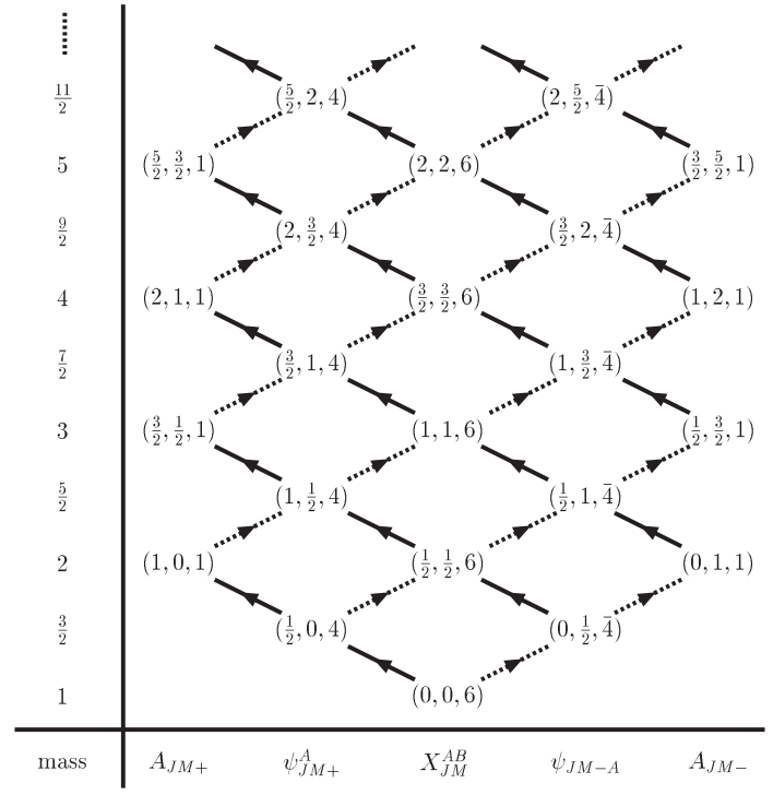
Figure 1: The KK tower of $\mathcal{N}=4$ super Yang-Mills on $R\times S^{3}$. The first number, the second number and the third number in the parentheses represent $J$, $\tilde{J}$ and the dimension of the representation of $SU(4)$, respectively. The solid and dotted arrows represent the superconformal transformation in the free theory for the creation operator caused by $\eta_{m+}$ and $\eta_{m-}^{*}$, respectively.

5 Consistent truncations

In this section we describe the consistent truncations of $\mathcal{N}=4$ SYM on $R\times S^{3}$ to the theories with 16 supercharges, in terms of the mode expansion performed in the previous section. This description helps us to extract various results for the theories with 16 supercharges from ones for $\mathcal{N}=4$ SYM on $R\times S^{3}$, such as the 1-loop hamiltonian for the $SO(6)$ sector (section 6) and the 1-loop effective action around a BPS solution (section 7). In section 5.1, we make the consistent truncations of $\mathcal{N}=4$ SYM on $R\times S^{3}$ to the theories with 16 supercharges in terms of the KK modes. In section 5.2, we compare the mass spectrum of $\mathcal{N}=4$ SYM on $R\times S^{2}$ with that of the theory obtained by quotienting the original theory by $U(1)$. We clarify how quotienting by $U(1)$ yields $\mathcal{N}=4$ SYM on $R\times S^{2}$. In section 5.3, we examine the vacua of $\mathcal{N}=4$ SYM on $R\times S^{2}$ in terms of the KK modes.

5.1 Consistent truncations to theories with 16 supercharges

The original SYM on $R\times S^{3}$ has the superconformal $SU(2,2|4)$, whose bosonic subgroup is $SO(2,4)\times SO(6)$. $SO(2,4)$ has a subgroup $SO(4)$ that is the isometry of the $S^{3}$ on which the theory defined. In section 2, we decomposed the $SO(4)$ as $SU(2)\times\tilde{SU}(2)$ and developed the harmonic expansion. We consider a subgroup of $\tilde{SU}(2)$. We project out all fields of $\mathcal{N}=4$ SYM on $R\times S^{3}$ which are not invariant under the subgroup of $\tilde{SU}(2)$ and consider the same interactions for the remaining fields as the ones in $\mathcal{N}=4$ SYM on $R\times S^{3}$. Taking full $\tilde{SU}(2)$, U(1), and $Z_{k}$ as the subgroup of $\tilde{SU}(2)$ leads to the plane wave matrix model, $\mathcal{N}=4$ SYM on $R\times S^{2}$ and $\mathcal{N}=4$ SYM on $S^{3}/Z_{k}$, respectively [1].

Let us describe the above truncations in terms of the KK modes. The plane wave matrix model is obtained by keeping only the modes that are singlet with respect to $\tilde{SU}(2)$, namely $(0,0,6)$ as ($X_{00}^{AB}$), $(\frac{1}{2},0,4)$ as ($\psi_{0M+}^{A}$) and $(1,0,1)$ as ($A_{0M+}$) in the KK tower[10]. The $\mathcal{N}=4$ SYM on $R\times S^{3}/Z_{k}$ is obtained by keeping only the modes with $\tilde{m}=\pm\frac{k}{2}q$, where $q\in\bm{Z}_{\geq 0}$. For later convenience, we examine the multiplicity of the remaining modes for fixed $\tilde{J}$. When $k$ is even, the remaining modes after the truncation have the following quantum numbers of $\tilde{SU}(2)$:

$$\tilde{J}=\frac{n}{2}+\frac{v}{2},$$ (5.1)

where $n\in\bm{Z}_{\geq 0}$ and $v=0,2,\cdots,k-2$, and

$$\tilde{m}=0,\pm\frac{k}{2},\cdots,\pm\frac{k}{2}n$$ (5.2)

for each $v$. Then the multiplicity of the remaining modes for fixed $n$ and $v$ is $2n+1$. Note that all the modes with $\tilde{J}$ a half odd integer should be projected out, because such modes cannot have $\tilde{m}=\frac{k}{2}\bm{Z}_{\geq 0}$.

In the odd $k$ case the discussion is similar to the above one. The quantum number $\tilde{J}$ for the remaining modes in this case takes the following values:

$$\tilde{J}=\frac{n}{2}+\frac{v}{2},$$ (5.3)

where $n\in\bm{Z}_{\geq 0}$ and $v=$ $0$, $1$, $\cdots$, $k-1$. Note that the range of $v$ for odd $k$ is different from that for even $k$. The values of $\tilde{m}$ and the multiplicity for fixed $n$ and $v$ are summarized in Table 1.

$n$	$v$	$\tilde{m}$	multiplicity
even	even	$0$, $\pm\frac{2k}{2}$ ,$\cdots$, $\pm\frac{nk}{2}$	$n+1$
even	odd	$\pm\frac{k}{2}$, $\pm\frac{3k}{2}$, $\cdots$, $\pm\frac{k}{2}(n-1)$	$n$
odd	even	$\pm\frac{k}{2}$, $\pm\frac{3k}{2}$, $\cdots$, $\pm\frac{k}{2}n$	$n+1$
odd	odd	$0$, $\pm\frac{2}{2}k$, $\cdots$, $\pm\frac{k}{2}(n-1)$	$n$

Table 1: The remaining modes for $\mathcal{N}=4$ SYM on $R\times S^{3}/Z_{k}$ for odd $k$.

The $\mathcal{N}=4$ SYM on $R\times S^{2}$ is obtained by keeping only the modes with $\tilde{m}=0$. We will discuss this truncation in the next subsection in detail.

We close this subsection by showing the consistency of the above truncations in terms of the KK modes. Let us first consider the cases of $\mathcal{N}=4$ SYM on $R\times S^{3}/Z_{k}$ and on $R\times S^{2}$. The conservation of $\tilde{m}$ implies that each term in the action of the original theory includes no KK mode or more than one KK mode that are projected out in the truncations. This fact ensures that the equation of motion in the original theory for a KK mode projected out in the truncations becomes trivial after the truncations. Hence, every classical solution of the truncated theories can be lifted up to a classical solution of the original theory.

In a similar way, one can show that the 16 supercharges for the supersymmetry transformations caused by $\eta_{m+}$ and $\eta_{m+}^{*}$ are preserved in the truncations. These parameters have $\tilde{m}=0$. The conservation of $\tilde{m}$ again implies that after the truncations the transformations of the KK modes that are projected out in the truncations become trivial and those of the remaining modes are still nontrivial. This means that the truncated theories have the 16 supercharges corresponding to $\eta_{m+}$ and $\eta_{m+}^{*}$.

In the case of the plane wave matrix model one must also use the conservation of $\tilde{J}$ to show the consistency of the truncation. Indeed the consistency of the truncation was checked explicitly in [10].

5.2 Comparison with $\mathcal{N}=4$ SYM on $R\times S^{2}$

In this subsection, we compare the remaining KK modes in the $U(1)$ truncation with the KK modes of $\mathcal{N}=4$ SYM on $R\times S^{2}$. Due to the mixing terms in $\mathcal{N}=4$ SYM on $R\times S^{2}$ this comparison is not trivial.

We begin by recalling the action of $\mathcal{N}=4$ SYM on $R\times S^{2}$ [6]

$$S_{2} = \frac{1}{g^{\prime 2}}\int dt\frac{d\Omega^{\prime}}{\mu^{2}}{\rm Tr}\bigg{\{}-\frac{1}{4}F_{a^{\prime}b^{\prime}}F^{a^{\prime}b^{\prime}}-\frac{1}{2}(D_{a^{\prime}}X_{m})^{2}-\frac{\mu^{2}}{8}X_{m}^{2}-\frac{1}{2}(D_{a^{\prime}}\Phi)^{2}-\frac{\mu^{2}}{2}\Phi^{2}$$ (5.4)

$$-\frac{i}{2}\bar{\lambda}\Gamma^{a^{\prime}}D_{a^{\prime}}\lambda+\frac{i\mu}{8}\bar{\lambda}\Gamma^{12\Phi}\lambda-\frac{1}{2}\bar{\lambda}\Gamma^{m}\left[X_{m},\lambda\right]+\frac{1}{2}\bar{\lambda}\Gamma^{\Phi}\left[\Phi,\lambda\right]$$

$$+\frac{1}{4}\left[X_{m},X_{n}\right]^{2}+\frac{1}{2}[\Phi,X_{m}]^{2}-\mu\Phi F_{12}\bigg{\}},$$

where $a^{\prime}=0,1,2$, and $m=1,\cdots,6$ and $(\Gamma^{a^{\prime}},\Gamma^{\Phi},\Gamma^{m})$ are ten dimensional gamma matrices. The radius of $S^{2}$ is $\mu^{-1}$ and the effective Yang-Mills coupling $g^{\prime 2}$ is defined by $g^{\prime 2}={g_{YM2}^{2}}/{4\pi}$, since the area of $S^{2}$ is $4\pi$ times square of the radius. We set $\mu=2$ since this value is obtained by the ${U}(1)$ truncating of $\mathcal{N}=4$ SYM on unit $S^{3}$. The volume integration over $S^{2}$ is normalized as

$$\int_{S^{2}}d\Omega^{\prime}=\int_{S^{2}}\frac{d\Omega_{2}}{4\pi\mu^{-2}}=1.$$ (5.5)

Note that the last term in (5.4) mixes $\Phi$ with $A_{a^{\prime}}$.

For later convenience we write down the mode expansion for the fields on $S^{2}$ here. The details for the harmonics on $S^{2}$ are left to appendix C. The mode expansions for the scalars, the vectors and the spinors on $S^{2}$ are given by

$$X_{AB}(t,\Omega^{\prime}) = \sum_{J\in\bm{Z}_{\geq 0}}\sum_{m=-J}^{J}X_{AB}^{Jm}(t){Y}_{Jm}(\Omega^{\prime}),\quad\Phi(t,\Omega^{\prime})=\sum_{J\in\bm{Z}_{\geq 0}}\sum_{m=-J}^{J}\Phi_{Jm}(t){Y}_{Jm}(\Omega^{\prime}),$$ (5.6)

$$A_{i}(t,\Omega^{\prime}) = \sum_{J\in\bm{Z}_{>0}}\sum_{m=-J}^{J}\Big{[}A_{Jm}^{t}(t){Y}_{Jmi}^{t}(\Omega^{\prime})+A_{Jm}^{l}(t)Y_{Jmi}^{l}(\Omega^{\prime})\Big{]}\quad(\mbox{for }i=1,2),$$ (5.7)

$$\psi_{\alpha}^{A}(t,\Omega^{\prime}) = \sum_{J\in\frac{1}{2}+\bm{Z}_{\geq 0}}\sum_{m=-J}^{J}\psi_{Jm}^{A\alpha}(t){Y}_{Jm\alpha}(\Omega^{\prime})\quad(\mbox{for }\alpha=\pm\frac{1}{2}),$$ (5.8)

where the spinor $\psi_{\alpha}^{A}$ is a two component one on $S^{2}$. Here $A_{Jm}^{t}$ and $A_{Jm}^{l}$ are the transverse and the longitudinal modes for the gauge fields. In the Coulomb gauge, the longitudinal modes ($A_{Jm}^{l}$) in (5.7) vanish because $\nabla_{i}A_{i}=0$ and $\nabla_{i}Y_{Jmi}^{t}=0$. Note that the range of $J$ is different form one for $S^{3}$, that is, $J$ takes zero and positive integers for the scalar, positive integers for the vector and positive half odd integers for the spinor. The hermicity of the fields implies together with (C.2) the following relations:

$$\left(X_{AB}^{Jm}\right)^{\dagger} = (-1)^{m}X^{AB}_{J-m},\qquad\left(\Phi_{Jm}\right)^{\dagger}=(-1)^{m}\Phi_{J-m},$$ (5.9)

$$\left(A_{Jm}^{t}\right)^{\dagger} = (-)^{-m}A_{J-m}^{t},\qquad\left(A_{Jm}^{l}\right)^{\dagger}=(-1)^{-m}A_{J-m}^{l}.$$ (5.10)

Let us first consider the spectrum of the $SO(6)$ scalar modes. In this case the comparison of the spectrum is straightforward. The mass term for the $SO(6)$ scalars in the $SU(4)$ notation is read off from (5.4) as

$$S_{X} = \int dtd\Omega^{\prime}{\rm Tr}\left\{\frac{1}{2}X_{m}\nabla^{2}X_{m}-\frac{\mu^{2}}{8}X_{m}^{2}\right\}$$ (5.11)

$$= \int dt\sum_{J\in\bm{Z}_{\geq 0}}\sum_{m=-J}^{J}\left\{-\frac{1}{2}\left[\mu\big{(}J+\frac{1}{2}\big{)}\right]^{2}{\rm Tr}\left\{(X_{Jm}^{AB})^{\dagger}X_{Jm}^{AB}\right\}\right\},$$

where in the second line we made the mode expansion by using (5.6) and used the formulae (C.2) and (C.3). It is clear that this equation is the same as the third line in (4.22)with the modes with integer $J$ and $\tilde{m}=0$ kept. Note that all the scalar modes with half odd integer $J$ in (4.22) should be projected out in this truncation because these modes cannot have $\tilde{m}=0$. The mass for the scalars on $S^{2}$ are immediately read off as $\mu(J+\frac{1}{2})$. The multiplicity for fixed $J$ is given by

$$\sum_{m=-J}^{J}1=2J+1.$$

The result is summarized in Table 2.

mass	multiplicity	$X_{JM}^{AB}$
$\mu(J+\frac{1}{2})$	$2J+1$	$(J,J,6)$

Table 2: The $SO(6)$ scalar mass spectrum of $\mathcal{N}=4$ SYM on $R\times S^{2}$ : The range of $J$ is $J\in\bm{Z}_{\geq 0}$. Note that $\mu=2$. The column of $X_{JM}^{AB}$ shows the corresponding $\mathcal{N}=4$ scalar modes on $S^{3}$ with the same mass.

We next consider the gauge field $A_{i}$ and the scalar $\Phi$ together. As mentioned before this comparison is not straightforward due to the mixing between $A_{i}$ and $\Phi$. We obtain their mass terms using the mode expansions (5.6) and (5.7) as follows:

$$S_{A\Phi} = \int dt{d\Omega^{\prime}}{\rm Tr}\left[\frac{1}{2}A_{i}\nabla^{2}A_{i}-\frac{\mu^{2}}{2}A_{i}A_{i}+\frac{1}{2}\Phi\nabla^{2}\Phi-\frac{\mu^{2}}{2}\Phi^{2}-\mu\Phi F_{12}\right]$$ (5.12)

$$= \int dt{\rm Tr}\left\{\frac{\mu^{2}}{2}\sum_{J\in\bm{Z}_{\geq 0}}\sum_{m=-J}^{J}\left[A_{JM}^{t\dagger},\Phi^{\dagger}_{Jm}\right]\left[\begin{array}[]{@{\,}cc@{\,}}-J(J+1)&\sqrt{J(J+1)}\\ \sqrt{J(J+1)}&-J(J+1)-1\end{array}\right]\left[\begin{array}[]{@{\,}c@{\,}}A_{Jm}^{t}\\ \Phi_{Jm}\end{array}\right]\right\}.$$ (5.17)

Here we took the Coulomb gauge, so that there is no longitudinal mode $A_{Jm}^{l}$ in this expression. A unitary matrix that diagonalizes the above mass matrix is given by

$$U=\frac{1}{\sqrt{2J+1}}\left[\begin{array}[]{@{\,}cc@{\,}}\sqrt{J+1}&-\sqrt{J}\\ +\sqrt{J}&\sqrt{J+1}\end{array}\right].$$ (5.20)

By redefining the modes for $A_{Jm}$ and $\Phi_{Jm}$ as

$$iA_{(J-1)m+} \equiv \sqrt{\frac{1+J}{1+2J}}A_{Jm}^{t}+\sqrt{\frac{J}{1+2J}}\Phi_{Jm},\qquad(\mbox{for }J\geq 1)$$ (5.21)

$$iA_{Jm-} \equiv -\sqrt{\frac{J}{1+2J}}A_{Jm}^{t}+\sqrt{\frac{1+J}{1+2J}}\Phi_{Jm},\qquad(\mbox{for }J\geq 0)$$ (5.22)

we find

$$S_{A\Phi}=\!\int\!dt\mbox{Tr}\left\{\!-\frac{1}{2}\sum_{J\in\bm{Z}_{\geq 0}}\sum_{m=-J-1}^{J+1}\mu^{2}(J+1)^{2}A_{Jm+}^{\dagger}A_{Jm+}-\frac{1}{2}\sum_{J\in\bm{Z}_{\geq 0}}\sum_{m=-J}^{J}\mu^{2}(J+1)^{2}A_{Jm-}^{\dagger}A_{Jm-}\!\right\}.$$

It is clear that this expression is the same as the second line in (4.22) with the modes with $\tilde{m}=0$ kept. Note that all the vector modes with half odd integer $J$ in (4.22) should be projected out in this truncation because these modes cannot have $\tilde{m}=0$. The result are summarized in Table 3.

mass	multiplicity	$A_{JM\pm}$
$\mu(J+1)$	$2J+1$	$(J,J+1,1)$
$\mu(J+1)$	$2J+3$	$(J+1,J,1)$

Table 3: The gauge boson and $\Phi$ mass spectrum of $\mathcal{N}=4$ SYM on $R\times S^{2}$ : The range of $J$ is $J\in\bm{Z}_{\geq 0}$. Note that $\mu=2$. The column of $A_{JM\pm}$ shows the corresponding gauge field modes on $S^{3}$ with the same mass.

Finally, in a similar way, we examine the mass spectrum of the fermions. The fermion mass term in (5.4) is

$$S_{\lambda} = \int dt{d\Omega^{\prime}}{\rm Tr}\left[-\frac{i}{2}\bar{\lambda}\Gamma^{i}\nabla_{i}\lambda+\frac{i\mu}{8}\bar{\lambda}\Gamma^{12\Phi}\lambda\right]=\int dtd\Omega^{\prime}{\rm Tr}\left[i\psi_{A}^{\dagger}\sigma^{i}\nabla_{i}\psi^{A}+\frac{\mu}{4}\psi_{A}^{\dagger}\psi^{A}\right]$$ (5.28)

$$= {\rm Tr}\int dt\sum_{J\in\frac{1}{2}+\bm{Z}_{\geq 0}}\sum_{m=-J}^{J}\mu\left[\psi_{JmA}^{1/2\dagger}\,\,\psi_{JmA}^{-1/2\dagger}\right]\left[\begin{array}[]{@{\,}cc@{\,}}\frac{1}{4}&J+\frac{1}{2}\\ J+\frac{1}{2}&\frac{1}{4}\end{array}\right]\left[\begin{array}[]{@{\,}c@{\,}}\psi_{Jm}^{\frac{1}{2}A}\\ \psi_{Jm}^{-\frac{1}{2}A}\end{array}\right],$$

In the first line we decomposed the sixteen component spinor $\lambda$ into the two component one $\psi_{\alpha}$ using (2.24) and (4.11). In the second line we made the mode expansion by using (5.8). Then a unitary matrix that diagonalize the fermion mass matrix in (5.28) is given by

$$V=\frac{1}{\sqrt{2}}\left[\begin{array}[]{@{\,}cc@{\,}}1&1\\ -1&1\end{array}\right].$$ (5.31)

After redefining the modes as

$$\psi_{(J-\frac{1}{2})(m,0)+}^{A}\equiv\frac{1}{\sqrt{2}}\left[\psi_{Jm}^{\frac{1}{2}A}-\psi_{Jm}^{-\frac{1}{2}A}\right],\qquad\psi_{J(m,0)-}^{A}\equiv\frac{1}{\sqrt{2}}\left[\psi_{Jm}^{\frac{1}{2}A}+\psi_{Jm}^{-\frac{1}{2}A}\right],$$ (5.32)

one finds

$$S_{\lambda} = \int dt{\rm Tr}\left\{\sum_{J\in\bm{Z}_{\geq 0}}\sum_{m=-J-\frac{1}{2}}^{J+\frac{1}{2}}-\mu\left[J+\frac{3}{4}\right]\psi_{J(m,0)+A}^{\dagger}\psi_{J(m,0)+}^{A}\right.$$ (5.33)

$$\left.+\sum_{J\in\frac{1}{2}+\bm{Z}_{\geq 0}}\sum_{m=-J}^{J}\mu\left[J+\frac{3}{4}\right]\psi_{J(m,0)-A}^{\dagger}\psi_{J(m,0)-}^{A}\right\}.$$

It is clear that this expression is the same as the forth line in (4.22) with the modes $\tilde{m}=0$ kept. The multiplicity for the modes with $J$ is $2J+1$. Notice that all the fermion mode $(J+\frac{1}{2},J,4)$ with half odd integer $J$ in (4.22) should be projected out because these modes cannot have $\tilde{m}=0$. For the same reason all the fermion mode $(J,J+\frac{1}{2},4)$ with integer $J$ in (4.22) should be projected out. The result for the fermion is summarized in Table 4.

$J$	mass	multiplicity	$\psi_{JM\pm}$
$J\in\bm{Z}_{\geq 0}$	$\mu(J+\frac{3}{4})$	$2J+2$	$(J+\frac{1}{2},J,4)$
$J\in\frac{1}{2}+\bm{Z}_{\geq 0}$	$\mu(J+\frac{3}{4})$	$2J+1$	$(J,J+\frac{1}{2},\bar{4})$

Table 4: The fermion mass spectrum of $\mathcal{N}=4$ SYM on $R\times S^{2}$ :The column of $\psi_{JM\pm}$ shows the corresponding fermion modes of $\mathcal{N}=4$ SYM on $R\times S^{3}$ with the same mass. Note that $\mu=2$.

5.3 Non-trivial vacua of $\mathcal{N}=4$ SYM on $R\times S^{2}$

It is discussed in [1] that $\mathcal{N}=4$ super Yang-Mills on $R\times S^{2}$ has many non-trivial vacua. Then it is valuable to describe these non-trivial vacua in terms of the modes to investigate the dynamics of this theory there, although we will study this theory in the trivial vacuum in this paper.

Let us start with writing down the potential terms in (5.4) that we focus on :

$$S_{pot}=\frac{1}{g^{\prime 2}\mu^{2}}\int dtd\Omega^{\prime}{\rm Tr}\left\{-\frac{1}{2}\Big{(}F_{12}+\mu\Phi\Big{)}^{2}-\frac{1}{2}\Big{(}\nabla_{i}\Phi-i\left[A_{i},\Phi\right]\Big{)}^{2}\right\}.$$ (5.34)

Because the potential consist of the sum of the two complete square terms, one immediately reads off the conditions for the zero-energy vacua:

$$F_{12}+\mu\Phi=0,$$ (5.35)

$$\nabla_{i}\Phi-i\left[A_{i},\Phi\right]=0\qquad(i=1,2).$$ (5.36)

These equations are rewritten in terms of the KK modes (5.6) and (5.7) as

$$-\mu\sqrt{J(J+1)}A_{Jm}^{t}+\mu\Phi_{Jm}+\frac{n_{J_{1}}^{0}n_{J_{2}}^{0}}{4n_{J}^{0}}\big{\{}1-(-1)^{J_{1}+J_{2}-J}\big{\}}C_{J_{1}1\,J_{2}-1}^{J0}C_{J_{1}m_{1}J_{2}m_{2}}^{Jm}\left[A_{J_{1}m_{1}}^{t},A_{J_{2}m_{2}}^{t}\right]=0,$$

(5.37)

$$\mu J(J+1)\Phi_{Jm}-\frac{n_{J_{1}}^{0}n_{J_{2}}^{0}}{2n_{J}^{0}}\sqrt{J_{2}(J_{2}+1)}\{1-(-1)^{J_{1}+J_{2}-J}\big{\}}C_{J_{1}1\,J_{2}-1}^{J0}C_{J_{1}m_{1}J_{2}m_{2}}^{Jm}\left[A_{J_{1}m_{1}}^{t},\Phi_{J_{2}m_{2}}\right]=0,$$

(5.38)

$$n_{J_{1}}^{0}n_{J_{2}}^{0}\{1+(-1)^{J_{1}+J_{2}-J}\big{\}}C_{J_{1}1\,J_{2}0}^{J1}C_{J_{1}m_{1}J_{2}m_{2}}^{Jm}\left[A_{J_{1}m_{1}}^{t},\Phi_{J_{2}m_{2}}\right]=0,$$ (5.39)

with no summation over $J$ and $m$. Here we took the Coulomb gauge $\nabla_{i}A_{i}=0$, so that there is no longitudinal mode $A_{Jm}^{l}$ in the above expressions. The equations (5.3) and (5.39) correspond to the longitudinal and transverse components of (5.36), respectively.

Unfortunately, it is difficult to find general solutions for (5.3)- (5.39). Then we would like to solve them with some assumptions. Let us first make an ansatz that the non-vanishing modes are only $A_{1m}$ and $\Phi_{1m}$ and that they are related as

$$\Phi_{1m}=\alpha A_{1m}^{t}.$$ (5.40)

Then it is easily verified using the relation $C^{Jm}_{1m_{1}1m_{2}}=(-1)^{1+1-J}C^{Jm}_{1m_{2}1m_{1}}$ that the equation (5.39) is trivially satisfied. When we set $\alpha=\frac{1}{\sqrt{2}}$, the equations (5.3) and (5.3) are reduced to three non-trivial ones:

$$\left[A_{10},A_{1\pm 1}\right]=\mp\sqrt{\frac{2}{3}}\mu A_{1\pm 1},\qquad\left[A_{11},A_{1-1}\right]=\sqrt{\frac{2}{3}}\mu A_{10}.$$ (5.41)

This is nothing but the $SU(2)$ algebra. Then the non-trivial solution is

$$A_{1-1}=\frac{\mu}{\sqrt{3}}L_{+},\quad A_{11}=-\frac{\mu}{\sqrt{3}}L_{-},\quad A_{10}=\sqrt{\frac{2}{3}}\mu L_{3},\quad\Phi_{1m}=\frac{1}{\sqrt{2}}A_{1m},$$ (5.42)

where $L_{i}$’s are the $SU(2)$ generators. It is easily checked that this solution are consistent with the hermicity conditions for the KK modes (5.9) and (5.10), of course, as it should be. When we consider the $\mathcal{N}=4$ $U(N)$ SYM on $R\times S^{2}$, our solution is expressed by an irreducible or reducible $SU(2)$ representation of dimension $N$. Then the number of the vacua that our solution (5.42) can represent is equal to the partitions of $N$, that is, $P(N)$. This number coincides with the number of vacua of the plane wave matrix model [1]. Note that our solution corresponds to a part of the solutions discussed in [6, 1], where the total number of the vacua of this theory and the tunneling amplitude between them are discussed.

6 1-loop calculations and the $SO(6)$ spin chains

In this section, we examine the 1-loop corrections. We consider those in the original theory in sections 6.1$\sim$6.3, and those in the truncated theories in section 6.4. In section 6.1, we illustrate the calculation of the 1-loop diagrams with the 1-loop self-energy of $X_{AB}$. In section 6.2, we introduce cut-offs for loop angular momenta as a regularization scheme and calculate the divergent parts of the self-energies of all the fields and some interaction vertices. We see that the coefficients of the logarithmic divergences are consistent with the vanishing of the beta function and the Ward identity. In section 6.3, we determine some 1-loop counter terms by examining the energy corrections of the BPS states. We examine the 1-loop energy corrections of the states that correspond to the operators on $R^{4}$ which are regarded as the integrable $SO(6)$ spin chain. We show that the energy corrections are actually given by the hamiltonian of the spin chain. In section 6.4, we determine some couter terms in the truncated theories by examining the 1-loop energy corrections of the BPS states. We find that the states viewed as the integrable $SO(6)$ spin chain in the original theory are also viewed as the same spin chain in the truncated theories.

6.1 Calculation of 1-loop diagrams

In the calculation of the 1-loop Feynman diagrams, we need the propagators, which are read off from (4.22) as

$$\langle X_{AB}^{JM}(q)_{kl}X_{A^{\prime}B^{\prime}}^{J^{\prime}M^{\prime}}(-q)_{k^{\prime}l^{\prime}}\rangle=\frac{1}{2}\varepsilon_{ABA^{\prime}B^{\prime}}(-1)^{m-\tilde{m}}\delta_{JJ^{\prime}}\delta_{M\>-M^{\prime}}\delta_{kl^{\prime}}\delta_{lk^{\prime}}\frac{i}{q^{2}-{\omega_{J}^{X}}^{2}},$$ (6.1)

$$\langle B_{JM}(q)_{kl}B_{J^{\prime}M^{\prime}}(-q)_{k^{\prime}l^{\prime}}\rangle=(-1)^{m-\tilde{m}}\delta_{JJ^{\prime}}\delta_{M\>-M^{\prime}}\delta_{kl^{\prime}}\delta_{lk^{\prime}}\frac{i}{4J(J+1)},$$ (6.2)

$$\langle A_{JM\rho}(q)_{kl}A_{J^{\prime}M^{\prime}\rho^{\prime}}(-q)_{k^{\prime}l^{\prime}}\rangle=(-1)^{m-\tilde{m}+1}\delta_{JJ^{\prime}}\delta_{M\>-M^{\prime}}\delta_{\rho\rho^{\prime}}\delta_{kl^{\prime}}\delta_{lk^{\prime}}\frac{i}{q^{2}-{\omega_{J}^{A}}^{2}},$$ (6.3)

$$\langle\psi_{JM\kappa}^{A}(q)_{kl}\psi_{J^{\prime}M^{\prime}\kappa^{\prime}A^{\prime}}^{\dagger}(q)_{k^{\prime}l^{\prime}}\rangle=\delta_{JJ^{\prime}}\delta_{MM^{\prime}}\delta^{A}_{\;A^{\prime}}\delta_{\kappa\kappa^{\prime}}\frac{i(q-\kappa\omega_{J}^{\psi})}{q^{2}-{\omega_{J}^{\psi}}^{2}},$$ (6.4)

$$\langle c_{JM}(q)_{kl}\bar{c}_{J^{\prime}M^{\prime}}(-q)_{k^{\prime}l^{\prime}}\rangle=(-1)^{m-\tilde{m}}\delta_{JJ^{\prime}}\delta_{M\>-M^{\prime}}\delta_{kl^{\prime}}\delta_{lk^{\prime}}\frac{1}{4J(J+1)},$$ (6.5)

where $q$ is conjugate to $t$.

(X-a)

(X-b)

(X-c)

(X-d)

(X-e)

(X-f)

Figure 2: Diagrams for the one-loop self-energy of $X_{AB}$. The curly line represents the propagator of $A_{i}$. The wavy line represents the propagator of $A_{0}$. The solid line represents the propagator of $X_{AB}$. The dashed line represents the propagator of $\psi^{A}$.

Here we consider the 1-loop self-energy of $X_{AB}$, which is $(-i)$ times the 1-loop contribution to the 1PI part of the truncated 2-point function $\langle X_{AB}^{JM}(q)_{kl}X_{A^{\prime}B^{\prime}}^{J^{\prime}M^{\prime}}(-q)_{k^{\prime}l^{\prime}}\rangle$. We will consider the self-energy of the other fields and the 1-loop corrections to some interaction vertices in the next subsection. The six diagrams for the self-energy of $X_{AB}$ are shown in Fig. 2. We illustrate our method by calculating one of the diagrams, $(X-f)$. By using the vertices in (4.23) and the propagator (6.4), we obtain an expression for this diagram.

$$4ig^{2}N\delta_{kl^{\prime}}\delta_{lk^{\prime}}\frac{1}{2}\varepsilon_{ABA^{\prime}B^{\prime}}\sum_{J_{1}M_{1}J_{2}M_{2}\kappa_{1}\kappa_{2}}$$

$$\times\int\frac{dp}{2\pi}\left(\frac{i(p-\kappa_{1}\omega_{J_{1}}^{\psi})}{p^{2}-{\omega_{J_{1}}^{\psi}}^{2}}\frac{i(-p+q-\kappa_{2}\omega_{J_{2}}^{\psi})}{(-p+q)^{2}-{\omega_{J_{2}}^{\psi}}^{2}}{\cal F}^{J_{1}\>-M_{1}\kappa_{1}}_{J_{2}M_{2}\kappa_{2}\;J-M}{\cal F}^{J_{2}M_{2}\kappa_{2}}_{J_{1}\>-M_{1}\kappa_{1}\;J^{\prime}-M^{\prime}}\right.$$

$$\qquad\qquad\;\;\;\left.+\frac{i(p-\kappa_{1}\omega_{J_{1}}^{\psi})}{p^{2}-{\omega_{J_{1}}^{\psi}}^{2}}\frac{i(-p-q-\kappa_{2}\omega_{J_{2}}^{\psi})}{(p+q)^{2}-{\omega_{J_{2}}^{\psi}}^{2}}{\cal F}^{J_{1}\>-M_{1}\kappa_{1}}_{J_{2}M_{2}\kappa_{2}\;J^{\prime}-M^{\prime}}{\cal F}^{J_{2}M_{2}\kappa_{2}}_{J_{1}\>-M_{1}\kappa_{1}\;J-M}\right)$$

$$=-8g^{2}N\delta_{kl^{\prime}}\delta_{lk^{\prime}}\frac{1}{2}\varepsilon_{ABA^{\prime}B^{\prime}}\sum_{J_{1}M_{1}J_{2}M_{2}\kappa_{1}}{\cal F}^{J_{1}M_{1}\kappa_{1}}_{J_{2}M_{2}\kappa_{1}\;J-M}{\cal F}^{J_{2}M_{2}\kappa_{1}}_{J_{1}M_{1}\kappa_{1}\;J^{\prime}-M^{\prime}}\frac{\omega_{J_{1}}^{\psi}+\omega_{J_{2}}^{\psi}}{q^{2}-(\omega_{J_{1}}^{\psi}+\omega_{J_{2}}^{\psi})^{2}}.$$

Here we plug in the expression for ${\cal F}$ in (B.21), take summations over $M_{1}$ and $M_{2}$ using the formulae (A.3) and (A.27). We also take a summation over $\kappa_{1}$ and plug in the expression for the $9-j$ symbol available in [32]. We eventually obtain

$$-16g^{2}N\delta_{kl^{\prime}}\delta_{lk^{\prime}}\frac{1}{2}\varepsilon_{ABA^{\prime}B^{\prime}}(-1)^{m-\tilde{m}}\delta_{JJ^{\prime}}\delta_{M-M^{\prime}}$$

$$\;\;\times\sum_{J_{1}J_{2}}\frac{(2J_{1}+2J_{2}+3)(J_{1}+J_{2}+J+2)(J_{1}+J_{2}-J+1)}{(q^{2}-(2J_{1}+2J_{2}+3)^{3})(2J+1)},$$ (6.7)

where $J_{1}$ and $J_{2}$ take non-negative half-integers $(0,\frac{1}{2},1,\frac{3}{2},\cdots,)$, and summations over $J_{1}$ and $J_{2}$ are taken such that they satisfy $|J_{1}-J_{2}|\leq J\leq J_{1}+J_{2}$. Because the summations give rise to divergence, we must introduce a regularization. In the next subsection, we give a method for regularization and calculate the divergent parts of the 1-loop diagrams.

In the following, we list unregularized expressions for all the diagrams in Fig. 2. The 1-loop self-energy of $X_{AB}$ takes the form

$$g^{2}N\delta_{kl^{\prime}}\delta_{lk^{\prime}}\frac{1}{2}\epsilon_{ABA^{\prime}B^{\prime}}(-1)^{m-\tilde{m}}\delta_{JJ^{\prime}}\delta_{M-M^{\prime}}\Pi^{X}_{J}(q).$$ (6.8)

We write down the contributions of each diagram to $\Pi^{X}_{J}(q)$.

$$(X-a)=\sum_{J_{1}\neq 0,J_{2}M_{1}M_{2}}\frac{i(-1)^{m_{1}-\tilde{m}_{1}+m_{2}-\tilde{m}_{2}}\delta(0)}{2J_{1}(J_{1}+1)}{\cal C}_{J\>-M\;J_{1}M_{1}\;J_{2}\>-M_{2}}{\cal C}_{J^{\prime}\>-M^{\prime}\;J_{1}\>-M_{1}\;J_{2}M_{2}},$$

$$(X-b)=-\sum_{J_{1}\neq 0,J_{2}M_{1}M_{2}}\frac{i(-1)^{m_{1}-\tilde{m}_{1}+m_{2}-\tilde{m}_{2}}\delta(0)}{2J_{1}(J_{1}+1)}{\cal C}_{J\>-M\;J_{1}M_{1}\;J_{2}\>-M_{2}}{\cal C}_{J^{\prime}\>-M^{\prime}\;J_{1}\>-M_{1}\;J_{2}M_{2}}$$

$$\qquad\qquad\;\;-\frac{1}{4}\sum_{J_{1}\neq 0,J_{2}}\frac{(2J_{1}+1)\left[q^{2}+(2J_{2}+1)^{2}\right]}{J_{1}(J_{1}+1)(2J+1)}\left\{J,J_{1},J_{2}\right\},$$

$$(X-c)=-2\sum_{J_{1}}\frac{(2J_{1}+1)(2J_{1}+3)}{2J_{1}+2},$$

$$(X-d)=-4\sum_{J_{1}J_{2}}$$

$$\qquad\qquad\;\;\frac{(2J_{1}+2J_{2}+3)(J+J_{1}+J_{2}+2)(J_{1}+J_{2}-J+1)(J-J_{1}+J_{2}+1)(J+J_{1}-J_{2})}{(2J+1)(J_{2}+1)^{2}\big{[}q^{2}-(2J_{1}+2J_{2}+3)^{2}\big{]}}$$

$$\qquad\qquad\;\;\times\{J,J_{1},J_{2}\}\{J,J_{1},J_{2}+1\},$$

$$(X-e)=-5\sum_{J_{1}J_{2}}\frac{2J_{2}+1}{2J+1}\left\{J,J_{1},J_{2}\right\},$$

$$(X-f)=-16\sum_{J_{1}J_{2}}\frac{(2J_{1}+2J_{2}+3)(J_{1}+J_{2}+J+2)(J_{1}+J_{2}-J+1)}{(2J+1)\big{[}q^{2}-(2J_{1}+2J_{2}+3)^{2}\big{]}}\{J,J_{1},J_{2}\}$$ (6.9)

where $\{J,J_{1},J_{2}\}$ represents the constraint $|J_{1}-J_{2}|\leq J\leq J_{1}+J_{2}$. Note that the terms proportional to $\delta(0)$ cancel in $(X-a)$ and $(X-b)$ [28]. We will later need the 1-loop on-shell self-energy for the lowest mode of $X_{AB}$, which is obtained by plugging in $q=1$ and $J=0$ into (6.9).

$$(X-a)+(X-b)=-\frac{1}{4}\sum_{J_{1}\neq 0}\frac{(2J_{1}+1)(1+(2J_{1}+1)^{2})}{J_{1}(J_{1}+1)},$$

$$(X-c)=-2\sum_{J_{1}}\frac{(2J_{1}+1)(2J_{1}+3)}{2J_{1}+2},$$

$$(X-d)=0,$$

$$(X-e)=-5\sum_{J_{1}}(2J_{1}+1),$$

$$(X-f)=4\sum_{J_{1}}(4J_{1}+3).$$ (6.10)

6.2 1-loop divergences and the Ward identity

All the expressions in (6.9) are divergent and must be regularized. As a regularization method, we introduce a cut-off for the loop angular momentum. Again, as an example, we explicitly regularize $(X-f)$. We introduce the cut-off $\Lambda_{f}$ for $J_{1}$. (Of course, we could introduce it for $J_{2}$.) The suffix ‘$f$’ indicates that the cut-off is the one for the loop of $\psi^{A}_{JM\kappa}$. Fig. 3 shows the region of the regularized summations over $J_{1}$ and $J_{2}$.

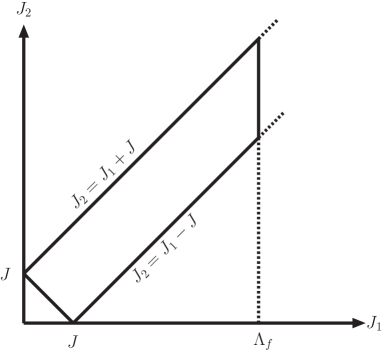
Figure 3: Region of the regularized summations over $J_{1}$ and $J_{2}$

We define new variables $P=J_{1}+J_{2}$ and $Q=J_{2}-J_{1}$, which take integers for integer $J$ and half odd integers for half odd integer $J$. Then, we obtain the regularized expression for $(X-f)$.

$$-16\left(\sum_{P=J}^{2\Lambda_{f}-J}\sum_{Q=-J}^{J}+\left.\sum_{r=-J+1}^{J}\sum_{Q=r}^{J}\right|_{P=2\Lambda_{f}+2r}\right)\frac{(2P+3)(P+J+2)(P-J+1)}{(q^{2}-(2P+3)^{2})(2J+1)}.$$ (6.11)

It is difficult to calculate this analytically, however the divergent part is easily evaluated as

$$8\sum_{P=J}^{2\Lambda_{f}-J}(P+\frac{3}{2})+16\sum_{r=-J+1}^{J}\sum_{Q=r}^{J}\frac{\Lambda_{f}}{2J+1}+2(q^{2}-(2J+1)^{2})\sum_{P=J}^{\Lambda_{f}-J}\frac{1}{P}$$

$$=16\Lambda_{f}^{2}+32\Lambda_{f}+2(q^{2}-(2J+1)^{2})\ln(2\Lambda_{f}).$$ (6.12)

We list the divergent parts of the expressions in (6.9).

$$(X-a)+(X-b)=-2\Lambda_{s}^{2}-3\Lambda_{s}+\left[-q^{2}-\frac{4}{3}J(J+1)-1\right]\log(2\Lambda_{s}),$$

$$(X-c)=-4\Lambda_{v}^{2}-10\Lambda_{v}+2\log(2\Lambda_{v}),$$

$$(X-d)=\frac{16}{3}J(J+1)\log(2\Lambda_{v}),$$

$$(X-e)=-10\Lambda_{s}^{2}-15\Lambda_{s},$$

$$(X-f)=16\Lambda_{f}^{2}+32\Lambda_{f}+2\left[q^{2}-(2J+1)^{2}\right]\log(2\Lambda_{f}),$$ (6.13)

where $\Lambda_{v}$ and $\Lambda_{s}$ represent the cut-off for the loop of $A_{JM\rho}$ and the cut-off for the loop of $X_{AB}^{JM}$ or $B_{JM}$, respectively. It is natural that $\Lambda_{s}$, $\Lambda_{v}$ and $\Lambda_{f}$ are the same order quantities, so that we can set $\log(2\Lambda_{s})=\log(2\Lambda_{v})=\log(2\Lambda_{f})=\log(2\Lambda)$ in the divergent parts. In appendix D, we list the divergent parts of the 1-loop self-energies of the other fields and those of the 1-loop corrections to some interaction vertices.

It should be remarked that all the 1-loop divergences here and in appendix D are local ones, namely they can be canceled by the local counter terms. This property is crucial in renormalizing the theory. In order to keep this property, one must introduce the cut-off for the angular momentum of a certain internal propagator in each diagram. For instance, one is not allowed to introduce the cut-offs for the angular momenta of several internal propagators or divide a contribution of a diagram into several parts and introduce the cut-off for the angular momentum of a different internal propagator in each part. Indeed, in the above example, we have introduced the cut-off $\Lambda_{f}$ only for $J_{1}$. Of course, the finite part as well as the divergent part in a 1-loop diagram generally depends on for which angular momentum the cut-off is introduced. As discussed in the following, however, this ambiguity does not matter. Our regularization method breaks the gauge symmetry and the superconformal symmetry though it preserves the $R\times SO(4)$ symmetry. As in [31], these symmetries would be recovered by introducing the counter terms that breaks the gauge invariance or the superconformal invariance and making the fine-tuning for the coefficients of these counter terms including the finite renormalization. Our gauge fixing also respects only $R\times SO(4)$ symmetry. We have to consider, therefore, all the terms whose dimension is less than or equal to four and which are invariant under $R\times SO(4)$, as the counter terms. The counter terms quadratic in $A_{i}$, $A_{0}$, $c$, $X_{AB}$ and $\psi^{A}$ take the following forms.

$$A_{i} : \alpha_{A}\mbox{Tr}\left(\frac{1}{2}(\partial_{0}A_{i})^{2}+\frac{1}{2}A_{i}\nabla^{2}A_{i}-A_{i}A_{i}\right)+\frac{\beta_{A}}{2}\mbox{Tr}(A_{i}\nabla^{2}A_{i}+2A_{i}A_{i})$$ (6.14)

$$-\gamma_{A}\mbox{Tr}(A_{i}A_{i}),$$

$$A_{0} : -\alpha_{B}\mbox{Tr}\left(\frac{1}{2}A_{0}\nabla^{2}A_{0}\right)+\frac{\gamma_{B}}{2}\mbox{Tr}(A_{0})^{2},$$ (6.15)

$$c : \alpha_{c}\mbox{Tr}(-i\bar{c}\nabla^{2}c)+\gamma_{C}\mbox{Tr}(\bar{c}c),$$ (6.16)

$$X_{AB} : \alpha_{X}\mbox{Tr}\left(\frac{1}{2}\partial_{0}X_{AB}\partial_{0}X^{AB}+\frac{1}{2}X_{AB}\nabla^{2}X^{AB}-\frac{1}{2}X_{AB}X^{AB}\right)$$ (6.17)

$$+\frac{\beta_{X}}{2}\mbox{Tr}(X_{AB}\nabla^{2}X^{AB})-\frac{\gamma_{X}}{2}\mbox{Tr}(X_{AB}X^{AB}),$$

$$\psi^{A} : \alpha_{\psi}\mbox{Tr}(i\psi^{\dagger}_{A}\partial_{0}\psi^{A}+i\psi^{\dagger}_{A}\sigma^{i}\nabla_{i}\psi^{A})+\beta_{\psi}\mbox{Tr}(i\psi^{\dagger}_{A}\sigma^{i}\nabla_{i}\psi^{A}).$$ (6.18)

The first term in each line is absorbed by the wave function renormalization of the corresponding field.

Let us see that our results of the 1-loop calculation are consistent with the vanishing of the beta function, which is characteristic of conformal field theories. We immediately see that the quadratic and linear divergences in (6.13) are absorbed in $\gamma_{X}$. The sum of the logarithmic divergences in (6.13) is $(q^{2}-{\omega_{J}^{X}}^{2})\log(2\Lambda)$. This shows that the cut-off dependent part of $\alpha_{X}$ is

$$\alpha_{X}\sim-\log(2\Lambda)g^{2}N.$$ (6.19)

Eqs.(D.2), (D.4), (D.6) and (D.8) in appendix D show the divergent parts of the diagrams for the 1-loop self-energies of $A_{i}$, $A_{0}$, $c$ and $\psi^{A}$, respectively. The quadratic and linear divergences in (D.2) and (D.4) are absorbed in $\gamma_{A}$ and $\gamma_{B}$, respectively, while the self-energies of $c$ and $\psi^{A}$ contain only the logarithmic divergences. The sum of the logarithmic divergences in (D.2) is $\frac{4}{3}(q^{2}-{\omega_{J}^{A}}^{2})\log(2\Lambda)$. The sum of those in (D.4) vanishes. The sum of those in (D.6) is $-\frac{8i}{3}J(J+1)\log(2\Lambda)$. The sum of those in (D.8) is $2(q+\kappa\omega_{J}^{\psi})\log(2\Lambda)$. All of these logarithmic divergences are absorbed by the wave function renormalization. We can determine the cut-off dependent parts of $\alpha_{A}$, $\alpha_{B}$, $\alpha_{c}$ and $\alpha_{\psi}$ as follows:

$$\alpha_{A}\sim-\frac{4}{3}\log(2\Lambda)g^{2}N,$$ (6.20)

$$\alpha_{B}\sim 0,$$ (6.21)

$$\alpha_{c}\sim\frac{2}{3}\log(2\Lambda)g^{2}N,$$ (6.22)

$$\alpha_{\psi}\sim-2\log(2\Lambda)g^{2}N.$$ (6.23)

As seen in (D.9), the diagrams for the 1-loop correction to the ghost-ghost-gauge interaction term are not divergent. The counter term proportional to $\mbox{Tr}(\nabla_{i}\bar{c}[A_{i},c])$ does not depend on the cut-off. This means together with (6.20) and (6.22) that the bare coupling constant can coincide with the renormalized one, namely the beta function vanishes. Similarly, the divergent parts of the diagrams for the 1-loop correction to the Yukawa interaction term are listed in (D.9) and contain only the logarithmic divergences. The sum of those divergences is $\frac{5}{2}\log(2\Lambda)$. The cut-off dependent part of the coefficient of the counter term proportional to $\mbox{Tr}(\psi^{\dagger}_{A}\sigma^{2}[X^{AB},(\psi^{\dagger}_{B})^{T}])$ is $-\frac{5}{2}\log(2\Lambda)g^{3}N$. This again means together with (6.19) and (6.23) that the beta function vanishes.

In general, the coefficients of the logarithmic divergences do not depend on the details of regularization, so that they respect the symmetries. This is consistent with the fact that we were able to check the vanishing of the beta function through the logarithmic divergences in our 1-loop calculation. Because our gauge choice only keeps the $R\times S^{3}$, it is difficult to examine the Ward identities for the superconformal symmetry. Here we content ourselves to see that the coefficients of the 1-loop logarithmic divergences satisfy the Ward identity for the gauge symmetry. As in [28], we consider the Ward identity in the flat limit that relates the 1-loop self-energy $\tilde{\Pi}_{ab}$ of the gauge field with the coefficient $\Phi^{a}$ of the $K_{a}c$ term in the 1-loop effective action, where $K_{a}$ is the source added for the operator $[Q_{BRST},c]$. It takes the form

$$\partial^{a}\tilde{\Pi}_{ab}+(\partial^{2}\eta_{ab}-\partial_{a}\partial_{b})\Phi^{a}=0.$$ (6.24)

As discussed above, the logarithmic divergent parts of $\tilde{\Pi}_{ab}$ and $\Phi_{a}$ should satisfy this identity. As explained in [28], the logarithmic divergent parts of $\tilde{\Pi}_{ab}$ take the forms

$$\tilde{\Pi}_{ij}^{div}=C((p_{0}^{2}-p_{k}p_{k})\delta_{ij}+p_{i}p_{j})g^{2}N\log(2\Lambda),$$

$$\tilde{\Pi}_{0i}^{div}=Dp_{i}p_{0}g^{2}N\log(2\Lambda),$$

$$\tilde{\Pi}_{00}^{div}=(-C+2D)p_{i}p_{i}g^{2}N\log(2\Lambda),$$ (6.25)

where $C$ and $D$ are certain numerical constants. The logarithmic divergent parts of $\Phi_{a}$ are determined by the Ward identity (6.24) as

$$\Phi_{0}^{div}=0,\;\;\;\;\;\Phi_{i}^{div}=(-C+D)p_{i}g^{2}N\log(2\Lambda).$$ (6.26)

We saw above that $C=\frac{4}{3}$ and $-C+2D=0$, namely $D=\frac{2}{3}$. In our case, $\Phi_{0}$ obviously vanishes and $\Phi_{i}$ is determined by calculating the diagram in Fig. 4. Its divergent part is

$$\int\!\!dtd\Omega\,{\rm Tr}\left(K_{i}\nabla_{i}c\right)\times\left[-\frac{2}{3}g^{2}N\log(2\Lambda)\right].$$ (6.27)

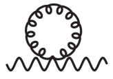
(B-a)

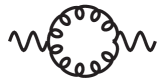
(B-b)

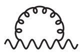
(B-c)

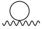
(B-d)

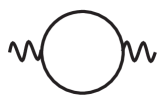
(B-e)

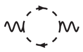
(B-f)

Figure 8: Diagrams for the one-loop self energy of $A_{0}$. The curly line represents the propagator of $A_{i}$. The solid line represents the propagator of $X_{AB}$. The dashed line represents the propagator of $\psi^{A}$.

This means $-C+D=-\frac{2}{3}$, which is indeed consistent with $C=\frac{4}{3}$ and $D=\frac{2}{3}$. We can also read off $C$ and $D$ for the pure Yang Mills sector by considering only $(A-a)\sim(A-f)$ in Fig. 7 and $(B-a)\sim(B-c)$ in Fig. 8. The result is $C=-\frac{1}{2}$ and $D=-\frac{7}{6}$ for the pure Yang Mills sector, which gives $-C+D=-\frac{2}{3}$ again. This is consistent because $\Phi_{a}$ for the pure Yang Mills sector is the same as that for ${\cal N}=4$ SYM. This consistency in pure Yang Mills is actually shown in [28].

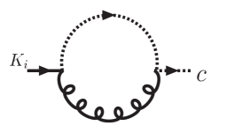
Figure 4: Diagram determining $\Phi_{i}$. The curly line represents the propagator of $A_{i}$. The dotted line represents the propagator of the ghost.

We close this subsection with an interesting observation. The quadratic and linear divergences appear in (6.13), (D.2) and (D.4). If we set

$$\Lambda_{v}=\Lambda_{s}-\frac{1}{2},\;\;\;\;\;\Lambda_{f}=\Lambda_{s}-\frac{1}{4},$$ (6.28)

those quadratic and linear divergences cancel and only the logarithmic divergences are left. Furthermore, these constant shifts of the cut-offs enable us to reproduce the Casimir energy in the free theory as follows. When we rewrote the naive expression to the normal ordered one in (4.30), we discarded the constant

$$N^{2}\left(2\sum_{J}(2J+1)(2J+3)\frac{1}{2}\omega_{J}^{A}+6\sum_{J}(2J+1)^{2}\frac{1}{2}\omega_{J}^{X}-8\sum_{J}(2J+1)(2J+2)\frac{1}{2}\omega_{J}^{\psi}\right),$$ (6.29)

where the first, second and third terms are the contributions of the gauge fields, the scalars and the fermions, respectively. Each term in (6.29) is quartic divergent in the angular momentum and must be regularized. If we set the upper end in the summation over $J$ in the first term at $\Lambda_{v}$, in the second term at $\Lambda_{s}$ and in the third term at $\Lambda_{f}$ and assume the above constant shifts of the cut-offs (6.28), we remarkably obtain the finite value, $\frac{3}{16}N^{2}$, which is independent of $\Lambda_{s}$. This is equal to the Casimir energy and is reasonably obtained as the zero point energy. The constant shifts of the cut-offs correspond to a complete specification of the regularization scheme. The physical meaning of these shifts is unclear at present and its understanding is an open problem. Here we only point out that these shifts are obtained by requiring that the average of $J$ and $\tilde{J}$ of the internal propagator agree for all the fields. That we are left only with the logarithmic divergences after the shifts of the cut-offs does not mean that we need no counter terms that break the gauge invariance. We need in general the finite couter terms that break the gauge invariance even in this situation.

6.3 Determination of counter terms and the $SO(6)$ spin chain

In this subsection, we obtain the 1-loop dilatation operator for the operators (4.31) in ${\cal N}=4$ SYM on $R^{4}$ by calculating the order $g^{2}N$ corrections to the energy of the states (4.32) in ${\cal N}=4$ SYM on $R\times S^{3}$. One can also consider the states (4.32) in the truncated theories. We show in the next subsection that the order $g^{2}N$ energy corrections of these states agree with that in the original theory, namely these states in the truncated theories are also regarded as the same integrable $SO(6)$ spin chain.

For the above purpose, we need the $\Pi^{X}_{J=0}(1)$, which is the coefficient of the on-shell self-energy for the lowest mode. The determination of this value is equivalent to fixing $\gamma_{X}$ in (6.17), because the first and second terms in (6.17) vanishes for $J=0$ and $q=1$. We determine this value by considering the BPS state. In addition, we similarly determine $\Pi^{A}_{J=0}(2)$ and $\Pi^{\psi}_{J=0}(-\frac{3}{2})$. The determination of the former is equivalent to fixing $\gamma_{A}$ in (6.14), while that of $\Pi^{\psi}_{J=0}(-\frac{3}{2})$ is equivalent to fixing $\beta_{\psi}$ in (6.18).

We consider the half-BPS state in the free theory, which corresponds to a special case with $l=2$ in (4.32):

$$\frac{2}{N}\mbox{Tr}(\alpha_{00}^{34\dagger}\alpha_{00}^{34\dagger})|0\rangle,$$ (6.30)

This state is mapped to the chiral primary operator $\mbox{Tr}((X^{34})^{2})$ on $R^{4}$. The energy of this state is 2. We also focus on the states that correspond to the descendant operators generated by the superconformal transformation caused by $\eta_{m+}$. Their forms are determined by (4.39) as

$$\frac{\sqrt{2}}{N}\mbox{Tr}(d_{0M}^{3\dagger}\alpha_{00}^{34\dagger})|0\rangle,\;\;\;\;\;\frac{\sqrt{2}}{N}\mbox{Tr}(d_{0M}^{4\dagger}\alpha_{00}^{34\dagger})|0\rangle,$$ (6.31)

$$\frac{1}{\sqrt{3}N}\mbox{Tr}(d^{3\dagger}_{0(\pm\frac{1}{2}0)}d^{4\dagger}_{0(\pm\frac{1}{2}0)}+2a_{0(\pm 10)+}^{\dagger}\alpha_{00}^{34\dagger})|0\rangle,$$ (6.32)

$$\frac{1}{\sqrt{6}N}\mbox{Tr}(d^{3\dagger}_{0(\frac{1}{2}0)}d^{4\dagger}_{0(-\frac{1}{2}0)}+d^{3\dagger}_{0(-\frac{1}{2}0)}d^{4\dagger}_{0(\frac{1}{2}0)}-2\sqrt{2}a_{0(00)+}^{\dagger}\alpha_{00}^{34\dagger})|0\rangle,$$ (6.33)

$$\frac{1}{N}\mbox{Tr}(d^{3\dagger}_{0(\pm\frac{1}{2}0)}d^{3\dagger}_{0(\mp\frac{1}{2}0)})|0\rangle,\;\;\;\;\;\frac{1}{N}\mbox{Tr}(d^{4\dagger}_{0(\pm\frac{1}{2}0)}d^{4\dagger}_{0(\mp\frac{1}{2}0)})|0\rangle,$$ (6.34)

$$\frac{1}{\sqrt{2}N}\mbox{Tr}(d^{3\dagger}_{0(\frac{1}{2}0)}d^{4\dagger}_{0(-\frac{1}{2}0)}-d^{3\dagger}_{0(-\frac{1}{2}0)}d^{4\dagger}_{0(\frac{1}{2}0)})|0\rangle.$$ (6.35)

The energy of (6.31) is $\frac{5}{2}$. The energy of (6.32), (6.33), (6.34) and (6.35) is 3. All the above states are half-BPS, and their energy must not receive any correction when the interactions are turned on. The BPS state (6.32) may mix with the non-BPS state whose energy is 3,

$$\sqrt{\frac{3}{2}}\frac{1}{N}\mbox{Tr}(d^{3\dagger}_{0(\pm\frac{1}{2}0)}d^{4\dagger}_{0(\pm\frac{1}{2}0)}-a_{0(\pm 10)+}^{\dagger}\alpha_{00}^{34\dagger})|0\rangle,$$ (6.36)

while the BPS state (6.33) may mix with the non-BPS state whose energy is 3,

$$\frac{1}{\sqrt{3}N}\mbox{Tr}(d^{3\dagger}_{0(\frac{1}{2}0)}d^{4\dagger}_{0(-\frac{1}{2}0)}+d^{3\dagger}_{0(-\frac{1}{2}0)}d^{4\dagger}_{0(\frac{1}{2}0)}+\sqrt{2}a_{0(00)+}^{\dagger}\alpha_{00}^{34\dagger})|0\rangle.$$ (6.37)

On the other hand, the BPS states (6.30), (6.31), (6.34) and (6.35) cannot mix with the other states.

We need to develop the hamiltonian formalism for the interacting theory to calculate the corrections to the energy. The canonical conjugate momenta obtained from (4.22), (4.23) and (4.24) have the corrections proportional to $g$, compared with those in the free energy, as follows.

$$P_{JM\rho}=\frac{\delta I}{\delta\dot{A}_{JM\rho}}=(-1)^{m-\tilde{m}+1}\dot{A}_{J-M\rho}-ig{\cal D}_{J_{1}M_{1}\;JM\rho\;J_{2}M_{2}\rho_{2}}[B_{J_{1}M_{1}},A_{J_{2}M_{2}\rho_{2}}],$$

$$P_{AB}^{JM}=\frac{\delta I}{\delta\dot{X}^{AB}_{JM}}=(-1)^{m-\tilde{m}}\dot{X}_{AB}^{J-M}-ig{\cal C}_{J_{1}M_{1}\;JM\;J_{2}M_{2}}[B_{J_{1}M_{1}},X^{AB}_{J_{2}M_{2}}],$$

$$P_{JM\kappa A}=\delta I/\delta\dot{\psi}^{A}_{JM\kappa}=i\psi^{\dagger}_{JM\kappa A}.$$ (6.38)

We solve the equations of motion for the auxiliary fields $B_{JM}$ and $c_{JM}$ iteratively with respect to $g$ and obtain

$$\hat{B}_{JM}=\frac{g}{4J(J+1)}\mbox{Tr}\left[(i(-1)^{m_{2}-\tilde{m}_{2}+1}{\cal D}^{JM}_{J_{1}M_{1}\rho_{1}\;J_{2}-M_{2}\rho_{2}}[A_{J_{1}M_{1}\rho_{1}},P_{J_{2}M_{2}\rho_{2}}]\right.$$

$$\qquad\quad\;\left.+i(-1)^{m_{2}-\tilde{m}_{2}}{\cal C}^{JM}_{J_{1}M_{1}\;J_{2}-M_{2}}[X^{AB}_{J_{1}M_{1}},P_{AB}^{J_{2}M_{2}}]+(-1)^{m-\tilde{m}}{\cal F}^{J_{2}M_{2}\kappa_{2}}_{J_{1}M_{1}\kappa_{1}\;J-M}\{\psi^{A}_{J_{1}M_{1}\kappa_{1}},\psi^{\dagger}_{J_{2}M_{2}\kappa_{2}A}\})\right]$$

$$\qquad\quad\;+{\cal O}(g^{2}),$$

$$\hat{c}_{JM}=0.$$ (6.39)

By substituting (6.38) and (6.39) into the hamiltonian,

$$H=\sum_{JM\rho}P_{JM\rho}\dot{A}_{JM\rho}+\sum_{JM}P_{AB}^{JM}\dot{X}^{AB}_{JM}+\sum_{JM\kappa}P_{JM\kappa A}\dot{\psi}^{A}_{JM\kappa}-L,$$ (6.40)

we obtain

$$H=H_{0}+H_{int},$$

$$H_{int}=-L_{int}^{(1)}+\sum_{J\neq 0,M}\frac{(-1)^{m-\tilde{m}}}{2}4J(J+1)\hat{B}_{J-M}\hat{B}_{JM}+{\cal O}(g^{3}),$$ (6.41)

where $H_{0}$ takes the same form as that in the free theory, and $L_{int}^{(1)}$ is given in (4.23).

In order to obtain the order $g^{2}N$ corrections to the energy, we calculate for the degenerate states, $|S_{n}\rangle$, the matrix elements

$$\Delta E^{g^{2}N}_{mn}=\langle S_{m}|H_{int,4}+H_{int,3}\frac{1-\sum_{n}|S_{n}\rangle\langle S_{n}|}{E_{0}-H_{0}}H_{int,3}+H_{2}^{1-loop}|S_{n}\rangle\equiv\langle S_{m}|H^{g^{2}N}_{eff}|S_{n}\rangle,$$ (6.42)

where $E_{0}$ is the unperturbed energy, and $H_{int,3}$ and $H_{int,4}$ is the 3-point and 4-point interaction terms in $H_{int}$, respectively, while $H_{2}^{1-loop}$ comes from the 1-loop counter terms quadratic in the fields and is proportional to $g^{2}N$.

We first calculate $H_{eff}^{g^{2}N}$ for the states (4.32). It is easy to see that the matrix elements among the states (4.32) with fixed $l$ are closed in the $g^{2}N$ corrections. As an example, let us see the contribution of the 4-point interaction in (6.41),

$$H_{int}^{X} = -\frac{g^{2}}{4}\int d\Omega\mbox{Tr}([X_{AB},X_{CD}][X^{AB},X^{CD}])$$ (6.43)

$$= -\frac{g^{2}}{2}{\cal C}^{j_{3}}_{j_{1}j_{2}}{\cal C}_{j_{3}j_{4}j_{5}}(\delta^{AB}_{EF}\delta^{CD}_{GH}-\delta^{AB}_{GH}\delta^{CD}_{EF})\mbox{Tr}(X_{AB}^{j_{1}}X_{CD}^{j_{2}}X^{EF}_{j_{4}}X^{GH}_{j_{5}}),$$

where we have introduced the abbreviated notations. $j$ represents a pair of $(J,M)$. $-j$ represents $(J,-M)$, and $j=0$ represents to $(J=0,M=0)$ in the following. We substitute

$$X^{AB}_{j}=\frac{1}{\sqrt{2\omega_{J}^{X}}}(\alpha^{AB}_{j}+(-1)^{m-\tilde{m}}\alpha^{AB\dagger}_{-j})$$ (6.44)

into (6.43). We take the Wick contractions to obtain the normal ordered form. After the contractions, we are forced to set $j=0$ for the creation and annihilation operators that are left in the normal ordering, because we consider the matrix elements among (4.32). The result is

$$H_{int}^{X}$$

$$=-\frac{g^{2}}{8}:\mbox{Tr}(2[\alpha_{0}^{AB\dagger},\alpha_{0}^{CD\dagger}][\alpha^{0}_{AB},\alpha^{0}_{CD}]-[\alpha_{0}^{AB\dagger},\alpha^{0}_{AB}][\alpha^{CD\dagger}_{0},\alpha^{0}_{CD}]+[\alpha_{0}^{AB\dagger},\alpha^{0}_{CD}][\alpha^{0\dagger}_{AB},\alpha^{CD}_{0}]):$$

$$\;\;\;+\frac{5g^{2}N}{2}\sum_{j_{2}j_{3}}\frac{(-1)^{m_{2}-\tilde{m}_{2}}}{\omega_{J_{2}}^{X}}{\cal C}^{j_{3}}_{0j_{2}}{\cal C}_{j_{3}-j_{2}0}:\mbox{Tr}(\alpha^{AB\dagger}_{0}\alpha^{0}_{AB}):$$

$$\;\;\;+\frac{15g^{2}N^{3}}{4}\sum_{j_{1}j_{2}j_{3}}\frac{(-1)^{m_{1}-\tilde{m}_{1}+m_{2}-\tilde{m}_{2}}}{\omega_{J_{1}}^{X}\omega_{J_{2}}^{X}}{\cal C}^{j_{3}}_{j_{1}j_{2}}{\cal C}_{j_{3}-j_{2}-j_{1}},$$ (6.45)

where $\alpha^{0}_{AB}\equiv\alpha^{(JM)=(00)}_{AB}$, and we have used ${\cal C}^{j_{3}}_{00}=1$ in the first term in the righthand side. We further evaluate the second term using $\sum_{M_{2}M_{3}}(-1)^{m_{2}-\tilde{m}_{2}}{\cal C}^{j_{3}}_{0j_{2}}{\cal C}_{j_{3}-j_{2}0}=(2J_{2}+1)^{2}\delta_{J_{2}J_{3}}$ and obtain

$$\frac{5g^{2}N}{2}\sum_{J_{2}}(2J_{2}+1):\mbox{Tr}(\alpha^{AB\dagger}_{0}\alpha^{0}_{AB}):,$$ (6.46)

We see from (6.10) that the coefficient of the number operator in (6.46) is nothing but $-\frac{g^{2}N}{2\omega_{J=0}^{X}}=-\frac{g^{2}N}{2}$ times the contribution of $(X-e)$ to $\Pi_{J=0}^{X}(1)$. Indeed, the contribution of the other 4-point interactions and the 3-point interactions to this coefficient correspond to the contribution of the other diagrams in (6.10). Note that the contribution of $(X-a)+(X-b)$ comes from the second term of $H_{int}$ in (6.41). Moreover, the contribution of $H_{2}^{1-loop}$ to this coefficient is $\frac{\gamma_{X}}{2}$. The third term in (6.45) is a constant that contributes equally to any $\langle S_{m}|H_{eff}^{g^{2}N}|S_{n}\rangle$. The sum of such constants that all the interactions yield must be zero due to the supersymmetry. We ignore these constants hereafter. As in [10], we rewrite $\mbox{Tr}([\alpha_{0}^{AB\dagger},\alpha^{0}_{AB}][\alpha^{CD\dagger}_{0},\alpha^{0}_{CD}])$ in the first term as

$$:\mbox{Tr}([\alpha_{0}^{AB\dagger},\alpha^{0}_{AB}]T^{a})::\mbox{Tr}(T^{a}[\alpha^{CD\dagger}_{0},\alpha^{0}_{CD}]):-2N:\mbox{Tr}(\alpha^{AB\dagger}_{0}\alpha^{0}_{AB}):,$$ (6.47)

where $T^{a}$ is the generators of $U(N)$. As shown in [10], the first term annihilates the states (4.32). We eventually obtain for the states (4.31)

$$H_{eff}^{g^{2}N} = \left(-\frac{g^{2}N}{2}\Pi_{J=0}^{X}(1)+\frac{1}{2}\gamma_{X}-\frac{g^{2}N}{4}\right):\mbox{Tr}(\alpha^{AB\dagger}_{0}\alpha^{0}_{AB}):$$ (6.48)

$$-\frac{g^{2}}{8}:\mbox{Tr}(2[\alpha_{0}^{AB\dagger},\alpha_{0}^{CD\dagger}][\alpha^{0}_{AB},\alpha^{0}_{CD}]+[\alpha_{0}^{AB\dagger},\alpha^{0}_{CD}][\alpha^{0\dagger}_{AB},\alpha^{CD}_{0}]):.$$

The expectation value of $H_{eff}^{g^{2}N}$ with respect to the state (6.30) must vanish, because it is BPS and does not mix with other states. The second term in (6.48) annihilates the state (6.30). Thus the coefficient of the number operator in the first term must vanish. Namely, $\gamma_{X}$ is determined as

$$\gamma_{X}=g^{2}N\left(\Pi_{J=0}^{X}(1)+\frac{1}{2}\right),$$ (6.49)

which in general depends on the cut-off and includes the finite renormalization.

The dilatation operator for the operators (4.31) on $R^{4}$ [30, 33] is

$$D_{2}=-\frac{g_{YM}^{2}}{32\pi^{2}}:\mbox{Tr}\left(2[X^{AB},X^{CD}][\frac{d}{dX^{AB}},\frac{d}{dX^{CD}}]+[X^{AB},\frac{d}{dX^{CD}}][X_{AB},\frac{d}{dX_{CD}}]\right):.$$ (6.50)

Recalling $g^{2}=\frac{g_{YM}^{2}}{4\pi^{2}}$ and comparing the remaining second term in (6.48) and (6.50), we find that the matrix elements of the order $g^{2}N$ corrections to the energy of the states (4.32) completely agree with those of the 1-loop dilatation operator for the operators (4.31), as expected.

Let us determine other counter terms. For the states (6.31),

$$H_{eff}^{g^{2}N} = \frac{g^{2}N}{4}:\mbox{Tr}(\alpha^{AB\dagger}_{0}\alpha^{0}_{AB}):+\left(g^{2}N\Pi_{J=0}^{\psi}(-\frac{3}{2})+\frac{3}{2}\beta_{\psi}\right):\mbox{Tr}(d^{A\dagger}_{m}d_{mA}):$$ (6.51)

$$+2g^{2}:\mbox{Tr}(d^{C\dagger}_{m}\alpha^{AB\dagger}_{0}d_{mA}\alpha_{BC}^{0}):,$$

where $d_{mA}\equiv d_{0(m,0)A}$ and $m$ takes $\pm\frac{1}{2}$. The states (6.31) do not mix with the other states, either. The expectation value of $H_{eff}^{g^{2}N}$ with respect to the states must vanish. It is evaluated as

$$\frac{g^{2}N}{4}+\left(g^{2}N\Pi_{J=0}^{\psi}(-\frac{3}{2})+\frac{3}{2}\beta_{\psi}\right)-g^{2}N=0,$$ (6.52)

from which we obtain

$$\beta_{\psi}=-\frac{2g^{2}N}{3}\Pi_{J=0}^{\psi}(-\frac{3}{2})+\frac{g^{2}N}{2}.$$ (6.53)

For the states (6.33)$\sim$(6.37),

$$H_{eff}^{g^{2}N} = \frac{g^{2}N}{4}:\mbox{Tr}(\alpha^{AB\dagger}_{0}\alpha^{0}_{AB}):+\frac{3g^{2}N}{4}:\mbox{Tr}(d^{A\dagger}_{m}d_{mA}):$$

$$+\left(-\frac{g^{2}N}{2\omega_{J=0}^{A}}\Pi_{J=0}^{A}(2)+\frac{\gamma_{A}}{\omega_{J=0}^{A}}\right):\mbox{Tr}(a^{\dagger}_{m}a_{m}):$$

$$-\frac{g^{2}}{4}:\mbox{Tr}(a_{m}^{\dagger}\alpha^{AB\dagger}_{0}a_{m}\alpha_{AB}^{0}):+\sqrt{6}g^{2}(-1)^{m_{1}+\frac{1}{2}}C^{\frac{1}{2}-m_{1}}_{\frac{1}{2}m_{2}\;1m_{3}}:\mbox{Tr}(d^{B\dagger}_{m_{2}}d^{A\dagger}_{m_{1}}\alpha_{AB}^{0}a_{m_{3}}):+(c.c.)$$

$$+\frac{g^{2}}{4}:\mbox{Tr}(d^{A\dagger}_{-m}d^{B\dagger}_{m}d_{-mA}d_{mB}-d^{A\dagger}_{m}d^{B\dagger}_{-m}d_{-mA}d_{mB}+d^{A\dagger}_{m}d^{B\dagger}_{m}d_{mB}d_{mA}+d^{A\dagger}_{m}d^{B\dagger}_{-m}d_{mB}d_{-mA}):,$$

where $a_{m}=a_{0(1m)+}$ and $m$ takes $0,\>\pm 1$. The matrix elements of $H_{eff}^{g^{2}N}$ among (6.32) and (6.36) form the $2\times 2$ matrix

$$\left(\begin{array}[]{cc}\frac{2}{3}(\chi-g^{2}N)&\frac{\sqrt{2}}{3}(\chi-g^{2}N)\\ \frac{\sqrt{2}}{3}(\chi-g^{2}N)&\frac{1}{3}(\chi+8g^{2}N)\end{array}\right),$$ (6.57)

where

$$\chi=-\frac{g^{2}N}{4}\Pi_{J=0}^{A}(2)+\frac{\gamma_{A}}{2}.$$ (6.58)

Those among (6.33) and (6.37) also form the same $2\times 2$ matrix. In order for the BPS energy not to receive any correction, one of the eigenvalues of this matrix must vanish. This is true if and only if $\chi=g^{2}N$, namely, we obtain

$$\gamma_{A}=g^{2}N\left(\frac{1}{2}\Pi_{J=0}^{A}(2)+2\right).$$ (6.59)

In this case, the other eigenvalue is $3g^{2}N$, and (6.32) and (6.33) are the eigenvector for the zero eigenvalue, while (6.36) and (6.37) are the eigenvector for the other eigenvalue. There is no correction to the BPS energy, and there is no mixing between the BPS and non-BPS states. It is also easy to see that the matrix elements among the BPS states (6.34) and (6.35), which have no mixing with the other states, vanish.

6.4 1-loop analysis of the truncated theories

So far we have been examining the 1-loop corrections in the original theory. It is easy to generalize the analysis in sections 6.1$\sim$6.3 to the 1-loop perturbation theory around the trivial vacua of the truncated theories. Consider the expression for a certain diagram in the original theory. By keeping only the KK modes to be remained in each truncated theory, in the external and internal propagators, one obtains the expression for the corresponding diagram in the truncated theory. The plane wave matrix model is at least perturbatively a finite theory, where no regularization is needed in the perturbative expansion, while ${\cal N}=4$ SYM on $R\times S^{2}$ and ${\cal N}=4$ SYM on $R\times S^{3}/Z_{k}$ give rise to divergences and must be regularized. In the perturbative expansion of the latters, as a regularization scheme, introducing the cut-offs for the loop angular momenta should be useful as in the original theory, although we have not explicitly calculated the divergent parts of the diagrams in those theories which are regularized in such a way. At any rate, we can proceed the following arguments assuming ${\cal N}=4$ SYM on $R\times S^{2}$ and ${\cal N}=4$ SYM on $R\times S^{3}/Z_{k}$ are appropriately regularized in terms of a certain regularization scheme.

One can also develop the hamiltonian formalism for the truncated theories. In particular, considering the states in (4.32) and (6.30)$\sim$(6.37) makes sence, because $X^{AB}_{00}$, $\psi_{0M+}$ and $A_{0M+}$ are remained in all the truncated theories although the correspondence with the operators on $R^{4}$ no longer exist. Furthermore, the truncated theories possess 16 supercharges, and the states (6.30)$\sim$(6.35) are also half-BPS, namely preserve 8 supercharges. Their mass spectrum must not receive any quantum correction. The mixing of these states with other states is the same as the original theory. The analysis of the $g^{2}N$ correction to the energy of the states (4.32) and (6.30)$\sim$(6.37) runs parallel to the one in the original theory, which is given below (6.42). It is easy to see that (6.48), (6.51) and (LABEL:HeffforE=3) hold for the truncated theories, and $\gamma_{X}$, $\beta_{\psi}$ and $\gamma_{A}$ are determined as (6.49), (6.53) and (6.59), respectively, in such a way that the supersymmetry is realized. Of course, the values of $\Pi_{J=0}^{X}(1)$, $\Pi_{J=0}^{\psi}(-\frac{3}{2})$ and $\Pi_{J=0}^{A}(2)$ depend on which theory is considered. In particular, in the plane wave matrix model, $\gamma_{X}$, $\beta_{\psi}$ and $\gamma_{A}$ are all zero, namely

$$\Pi_{J=0}^{X}(1)=-\frac{1}{2},\;\;\;\;\;\Pi_{J=0}^{\psi}(-\frac{3}{2})=\frac{3}{4},\;\;\;\;\;\Pi_{J=0}^{A}(2)=-4$$ (6.60)

must hold. Indeed, from (6.10), we can calculate the contribution of each diagram to $\Pi_{J=0}^{X}$ as

$$(X-c)=-\frac{3}{2},\;\;\;\;\;(X-e)=-5,\;\;\;\;\;(X-f)=6,$$ (6.61)

The total of these values amounts to $-\frac{1}{2}$. Note that the diagrams $(X-a)$, $(X-b)$, $(X-d)$ and $(X-g)$ do not exist in this theory. Similarly, we obtained $\Pi_{J=0}^{\psi}(-\frac{3}{2})$ and $\Pi_{J=0}^{A}(2)$ in (6.60) by calculating the diagrams in the plane wave matrix model.

The above arguments lead us to a following interesting conclusion. In the truncated theories, the matrix elements of the $g^{2}N$ corrections to the energy of the states (4.31) are mapped to the hamiltonian of the same integrable $SO(6)$ spin chain that appear in the original theory. Indeed, the authors of [9] verified this fact in the plane wave matrix model by direct calculation. In [9], the matrix elements of (6.51) in the plane wave matrix model are also obtained by direct calculation, and are consistent with the above arguments.

As a side remark, we checked that as in the original theory by making shifts of the cut-offs in (6.28) one can obtain the finite zero point energy in the truncated theories with $g=0$. Its value is zero for ${\cal N}=4$ SYM on $R\times S^{2}$ and $\frac{3}{16k}N^{2}$ for ${\cal N}=4$ SYM on $R\times S^{3}/Z_{k}$. These two values are consistent, since in the $k\rightarrow\infty$ limit ${\cal N}=4$ SYM on $R\times S^{3}/Z_{k}$ is reduced to ${\cal N}=4$ SYM on $R\times S^{2}$ [1].

7 Time-dependent BPS solution

In this section, we examine a classical time-dependent BPS solution and the 1-loop effective action around it in the original and truncated theories. In section 7.1, we construct the time-dependent BPS solution of the original and truncated theories. In section 7.2, we calculate the 1-loop effective action around it in the original theory, and in section 7.3 that in the truncated theories.

7.1 Classical time-dependent BPS solution

We consider a configuration in which all the KK modes and matrix components except the $(1,1)$ component of $X_{34}^{00}$ vanish. Namely,

$$X_{34}^{00}=X^{12}_{00}=(X^{34})^{\dagger}=(X_{12}^{00})^{\dagger}=\left(\begin{array}[]{cccc}\frac{1}{2}\rho(t)\>e^{i\eta(t)}&0&\cdots&0\\ 0&0&\cdots&0\\ \vdots&\vdots&&\vdots\\ 0&0&\cdots&0\end{array}\right).$$ (7.5)

It is easy to see that this assumption is a consistent truncation in the original and truncated theories. Under this assumption, the classical action becomes

$$S_{c}=\int dt\>\frac{1}{2}(\dot{\rho}^{2}+\rho^{2}\dot{\eta}^{2}-\rho^{2}).$$ (7.6)

The canonical momenta are read off as

$$p_{\rho}=\frac{\delta S_{c}}{\delta\dot{\rho}}=\dot{\rho},$$

$$l=\frac{\delta S_{c}}{\delta\dot{\eta}}=\rho^{2}\dot{\eta}.$$ (7.7)

The angular momentum in the $(6,9)$ plane, $l$, is conserved and corresponds to the R charge (Recall $X_{34}=(X_{6}+iX_{9})/2$). The energy possesses the BPS bound:

$$E=\frac{1}{2}{p_{\rho}}^{2}+\frac{l^{2}}{2\rho^{2}}+\frac{1}{2}\rho^{2}\geq|l|$$ (7.8)

When $p_{\rho}=0$ and $l^{2}=\rho^{4}$, the BPS bound is saturated. In this case, $\rho=\sqrt{|l|}=\mbox{const.}$ and $\eta=\pm t+\mbox{const.}$. We can set $\rho=\sqrt{l}$ and $\eta=t$ without loss of generality. That is, we consider the solution

$$(X_{34}^{00})_{11}=\frac{1}{2}\sqrt{l}\>e^{it}.$$ (7.9)

For this solution, non-vanishing elements in (2.34) are

$$\delta_{\epsilon}(\lambda_{+}^{A})_{11}=2(\partial_{0}(X^{AB})_{11}\mp i(X^{AB})_{11})\gamma^{0}\epsilon_{-B},$$

$$\delta_{\epsilon}(\lambda_{-A})_{11}=2(\partial_{0}(X_{AB})_{11}\pm i(X_{AB})_{11})\gamma^{0}\epsilon_{+}^{B}.$$ (7.10)

The requirement $\delta_{\epsilon}\lambda_{+}^{A}=0$ and $\delta_{\epsilon}\lambda_{-A}=0$ leads to $\epsilon_{-3}=\epsilon_{+}^{3}=\epsilon_{-4}=\epsilon_{+}^{4}=0$ for the upper sign and $\epsilon_{-1}=\epsilon_{+}^{1}=\epsilon_{-2}=\epsilon_{+}^{2}=0$ for the lower sign. The solution is, therefore, a half BPS solution. It preserves 16 supercharges for the original theory and 8 supercharges for the truncated theories. The BPS solution corresponds to a circular motion in the $(6,9)$ plane (see Fig. 6) while generic non-BPS solutions correspond to elliptical motions (see Fig. 6). The BPS solution is the classical counterpart of the lowest Landau level in the Landau problem. The BPS solution is interpreted as the AdS giant graviton in the original theory [18], and corresponds to a particular one of the spherical membrane solutions in the plane wave matrix model, which were studied in [5].

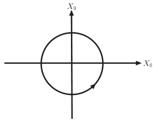
Figure 5: BPS solution

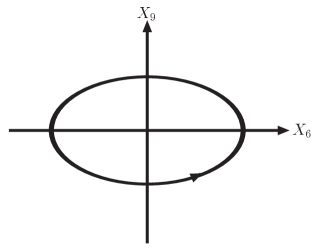
Figure 6: Non-BPS solution

7.2 1-loop effective action around the solution in the original SYM

We calculate the 1-loop effective action around the BPS solution in the original ${\cal N}=4$ SYM, which was obtained in the previous subsection. Following the background field method, we make a substitution

$$(X_{34})_{kl}\rightarrow\frac{1}{2}\sqrt{l}e^{it}\delta_{k1}\delta_{l1}+(X_{34})_{kl},$$

$$(X_{12})_{kl}\rightarrow\frac{1}{2}\sqrt{l}e^{-it}\delta_{k1}\delta_{l1}+(X_{12})_{kl}$$ (7.11)

in the gauge-fixed action $I$ and keep the second-order in all fields. Then we immediately see that $I_{int}$ are only written by the $(1,k)$ and $(k,1)$ components, where $k\neq 1$, and as far as the other components are concerned, $I$ takes the same form as the free theory. We can therefore forget the contribution of the other components. Moreover, the fields with different $k$’s are decoupled and $I$ takes the same form for each $k$. We can calculate the effective action for a fixed $k$ and multiply the result by $N-1$ to obtain the final answer. (In the ’t Hooft limit, the factor $N-1$ can be replaced with $N$.) We omit the suffices for the matrix components and absorb explicit time dependence into the fields:

$$(X_{34})_{1k}\rightarrow\frac{1}{\sqrt{2}}e^{it}Z_{1},\;\;\;(X_{12})_{1k}\rightarrow\frac{1}{\sqrt{2}}e^{-it}Z_{2}^{\ast},$$

$$(X_{24})_{1k}\rightarrow\frac{1}{\sqrt{2}}Y_{1},\;\;\;(X_{31})_{1k}\rightarrow\frac{1}{\sqrt{2}}Y_{2}^{\ast},\;\;\;(X_{14})_{1k}\rightarrow\frac{1}{\sqrt{2}}Y_{3},\;\;\;(X_{23})_{1k}\rightarrow\frac{1}{\sqrt{2}}Y_{4}^{\ast},$$

$$(A_{0})_{1k}\rightarrow A_{0},\;\;\;(A_{i})_{1k}\rightarrow A_{i},$$

$$(\psi^{3})_{1k}\rightarrow e^{-\frac{i}{2}t}\varphi_{1},\;\;\;(\psi_{3}^{\dagger T})_{1k}^{\ast}\rightarrow e^{-\frac{i}{2}t}\varphi_{2},\;\;\;(\psi^{4})_{1k}\rightarrow e^{-\frac{i}{2}t}\varphi_{3},\;\;\;(\psi_{4}^{\dagger T})_{1k}^{\ast}\rightarrow e^{-\frac{i}{2}t}\varphi_{4},$$

$$(\psi^{1})_{1k}\rightarrow e^{\frac{i}{2}t}\phi_{5},\;\;\;(\psi_{1}^{\dagger T})_{1k}^{\ast}\rightarrow e^{\frac{i}{2}t}\varphi_{6},\;\;\;(\psi^{2})_{1k}\rightarrow e^{\frac{i}{2}t}\varphi_{7},\;\;\;(\psi_{2}^{\dagger T})_{1k}^{\ast}\rightarrow e^{\frac{i}{2}t}\varphi_{8}.$$ (7.12)

The resultant quadratic action is

$$I=\frac{1}{g^{2}}\int dtd\Omega\left[\sum_{r=1,2}Z_{r}^{\ast}(-\partial_{0}^{2}-2i\partial_{0}+\nabla^{2}-\frac{l}{2})Z_{r}+\frac{l}{2}(Z_{1}^{\ast}Z_{2}^{\ast}+Z_{1}Z_{2})\right.$$

$$\qquad+\sum_{r=1}^{4}Y_{r}^{\ast}(-\partial_{0}^{2}+\nabla^{2}-1-l)Y_{r}+A_{0}^{\ast}(-\nabla^{2}+l)A_{0}$$

$$\qquad+\sqrt{2l}(A_{0}(Z_{1}^{\ast}-Z_{2})+A_{0}^{\ast}(Z_{1}-Z_{2}^{\ast}))+i\sqrt{\frac{l}{2}}(A_{0}(\partial_{0}Z_{1}^{\ast}+\partial_{0}Z_{2})-A_{0}^{\ast}(\partial_{0}Z_{1}+\partial_{0}Z_{2}^{\ast}))$$

$$\qquad+A_{i}^{\ast}(-\partial_{0}^{2}+\nabla^{2}-2-l)A_{i}+\sum_{s=1}^{8}\varphi_{s}^{\dagger}(i\partial_{0}+i\sigma^{i}\nabla_{i})\varphi_{s}+\frac{1}{2}\sum_{s=1}^{4}\varphi_{s}^{\dagger}\varphi_{s}-\frac{1}{2}\sum_{s=5}^{8}\varphi_{s}^{\dagger}\varphi_{s}$$

$$\qquad+\sqrt{l}(\varphi_{4}^{\dagger}\sigma^{2}\varphi_{1}^{\dagger T}+\varphi_{4}^{T}\sigma^{2}\varphi_{1}-\varphi_{2}^{\dagger}\sigma^{2}\varphi_{3}^{\dagger T}-\varphi_{2}^{T}\sigma^{2}\varphi_{3}$$

$$\qquad\quad\;\;\;\left.+\varphi_{8}^{\dagger}\sigma^{2}\varphi_{5}^{\dagger T}+\varphi_{8}^{T}\sigma^{2}\varphi_{5}-\varphi_{6}^{\dagger}\sigma^{2}\varphi_{7}^{\dagger T}-\varphi_{6}^{T}\sigma^{2}\varphi_{7})\right].$$ (7.13)

Note that the ghosts do not contribute to this calculation of the 1-loop effective action because of the Coulomb gauge. We must also take into account the contribution of the 1-loop counter terms consisting only of $X^{AB}$. We substitute the background in (7.11) into them. As far as the counter terms quadratic in $X^{AB}$ (6.17) are concerned, there is the contribution only from $-\frac{\gamma_{X}}{2}\mbox{Tr}(X_{AB}X^{AB})$, which results in $-\int dt\frac{\gamma_{X}}{2}l$, where $\gamma_{X}$ is given in (6.49). We will see below that this contribution is consistently needed for vanishing of the 1-loop effective action around the time-dependent BPS solution. Among possible counter terms quartic in $X^{AB}$, the single trace ones are

$$\mbox{Tr}([X_{AB},X_{CD}][X^{AB},X^{CD}]),$$ (7.14)

$$\mbox{Tr}(X_{AB}X^{AB}X_{CD}X^{CD}),$$ (7.15)

and the double trace ones are

$$\frac{1}{N}\mbox{Tr}(X_{AB}X^{AB})\mbox{Tr}(X_{CD}X^{CD}),\;\;\;\;\;\frac{1}{N}\mbox{Tr}(X_{AB}X_{CD})\mbox{Tr}(X^{AB}X^{CD}).$$ (7.16)

(7.14) vanishes when the background is plugged in, while the double trace ones (7.16) do not contribute in this case due to $1/N$ suppression. We can, therefore, determine the coefficient of (7.15) from the requirement of vanishing of the 1-loop effective action.

We make a mode expansion for all fields in (7.13). We first integrate over $A_{0}$ and obtain new terms that are quadratic in $Z_{r}$ and $Z_{r}^{\ast}$. After the redefinition, $(-1)^{m-\tilde{m}}Z_{2}^{JM}\rightarrow Z_{2}^{JM}$, the action concerning $Z_{r}$ and $Z_{r}^{\ast}$ becomes

$$\frac{1}{g^{2}}\int dt\left[{Z_{1}^{00}}^{\ast}(-\partial_{0}^{2}-2i\partial_{0}-\frac{1}{2}l)Z_{1}^{00}+{Z_{2}^{00}}^{\ast}(-\partial_{0}^{2}+2i\partial_{0}-\frac{1}{2}l)Z_{2}^{00}\right.$$

$$\left.+\frac{1}{2}l({Z_{1}^{00}}^{\ast}{Z_{2}^{00}}^{\ast}+Z_{1}^{00}Z_{2}^{00})\right]$$

$$+\sum_{J\neq 0,M}\int dt\left[{Z_{1}^{JM}}^{\ast}(-(1-K_{J})\partial_{0}^{2}-2i(1-2K_{J}))\partial_{0}-({\omega_{J}^{X}}^{2}-1+\frac{1}{2}l+4K_{J})Z_{1}^{JM}\right.$$

$$+{Z_{2}^{J\>-M}}(-(1-K_{J})\partial_{0}^{2}+2i(1-2K_{J}))\partial_{0}-({\omega_{J}^{X}}^{2}-1+\frac{1}{2}l+4K_{J}){Z_{2}^{J\>-M}}^{\ast}$$

$$\left.+{Z_{1}^{JM}}^{\ast}(K_{J}\partial_{0}^{2}+\frac{1}{2}l+4K_{J}){Z_{2}^{J\>-M}}^{\ast}+Z_{2}^{J\>-M}(K_{J}\partial_{0}^{2}+\frac{1}{2}l+4K_{J})Z_{1}^{JM}\right],$$ (7.17)

where

$$K_{J}=\frac{l}{2}\frac{1}{4J(J+1)+l}.$$ (7.18)

In order to evaluate the 1-loop effective action, we use a formula

$$\mbox{Tr}\ln(\partial_{0}^{2}-2ip\partial_{0}+m^{2})=i\int dt\sqrt{p^{2}+m^{2}}.$$ (7.19)

It is easy to see that the contribution of $Z_{1}^{00}$ and $Z_{2}^{00}$ to the effective action is

$$\Gamma_{eff}^{Z0}=-g^{2}N\int dt\sqrt{4+l},$$ (7.20)

and the contribution of $Z_{1}^{JM}$ and $Z_{2}^{JM}$ $((JM)\neq(00))$ is

$$\Gamma_{eff}^{Z} = -g^{2}N\int dt\sum_{(JM)\neq(00)}(\sqrt{4J^{2}+l}+\sqrt{(2J+2)^{2}+l}\>)$$ (7.21)

$$= -g^{2}N\int dt\sum_{J\neq 0}(2J+1)^{2}(\sqrt{4J^{2}+l}+\sqrt{(2J+2)^{2}+l}\>).$$

We can evaluate the contribution of $Y_{r}$, $A_{i}$ and the fermions in a similar way. The contribution of $Y_{r}$ is

$$\Gamma_{eff}^{Y}=-4g^{2}N\int dt\sum_{J}(2J+1)^{2}\sqrt{(2J+1)^{2}+l}.$$ (7.22)

The contribution of $A_{i}$ is

$$\Gamma_{eff}^{A}=-2g^{2}N\int dt\sum_{J}(2J+1)(2J+3)\sqrt{(2J+2)^{2}+l}.$$ (7.23)

The contribution of the fermions is

$$\Gamma_{eff}^{F}=4g^{2}N\int dt\sum_{J}(2J+1)(2J+2)(\sqrt{(2J+2)^{2}+l}+\sqrt{(2J+1)^{2}+l}\>).$$ (7.24)

We also have the contribution of the 1-loop counter term, $-\frac{\gamma_{X}}{2}\mbox{Tr}(X_{AB}X^{AB})$,

$$\Gamma_{eff}^{c.t.(1)}=-g^{2}N\int dt\frac{l}{2}\left(\Pi_{J=0}^{X}(1)+\frac{1}{2}\right).$$ (7.25)

Besides, there can be a contribution of the 1-loop counter term (7.15), which is quadratic in $l$ and denoted by $\Gamma_{eff}^{c.t.(2)}$. We denote the sum of all the contribution by $\Gamma_{eff}$:

$$\Gamma_{eff}=\Gamma_{eff}^{Z0}+\Gamma_{eff}^{Z}+\Gamma_{eff}^{Y}+\Gamma_{eff}^{A}+\Gamma_{eff}^{F}+\Gamma_{eff}^{c.t.(1)}+\Gamma_{eff}^{c.t.(2)}.$$ (7.26)

Let us see that the sum of (7.20)$\sim$(7.24) vanishes. First, comparing the order $l^{0}$ contribution in (7.20)$\sim$(7.24) with (6.29), we find that it is nothing but the contribution of the $(1,k)$ and $(k,1)$ components of the fields to the zero point energy, and we can ignore it here. Next, the order $l^{1}$ contribution is evaluated as follows (we omit the common factor $lg^{2}N\int dt$):

$$\Gamma_{eff}^{Z0} \rightarrow -\frac{1}{4},$$

$$\Gamma_{eff}^{Z} \rightarrow -\frac{1}{4}\sum_{J\neq 0}\frac{(2J+1)^{3}}{J(J+1)},$$

$$\Gamma_{eff}^{Y} \rightarrow -2\sum_{J}(2J+1),$$

$$\Gamma_{eff}^{A} \rightarrow -\sum_{J}\frac{(2J+1)(2J+3)}{2J+2},$$

$$\Gamma_{eff}^{F} \rightarrow 2\sum_{J}(4J+3).$$ (7.27)

Comparing (7.27) with (6.10), we find that the total of (7.27) is equal to

$$\frac{1}{2}\Pi_{J=0}^{X}(1)+\frac{1}{4}.$$ (7.28)

This is canceled by (7.25). Namely, we find

$$\mbox{the order $l^{1}$ contribution in }\Gamma_{eff}=0.$$ (7.29)

Note that the righthand sides in (7.27) except the first line have correspondence with those in (6.10). If this correspondence also held for the first line in (7.27), the order $l^{1}$ contribution in $\Gamma_{eff}^{Z0}$ would be $-\frac{1}{2}$ rather than $-\frac{1}{4}$ and the total of the righthand sides in (7.27) would agree with $\frac{1}{2}\Pi_{J=0}^{X}(1)$. This agreement is naively anticipated because the background field method usually gives the generating function of the 1PI diagrams. However, this is not true in this case. Our result shows that in this case the loop expansion and the expansion in $l$ do not commute.

Finally the order $l^{2}$ contribution in (7.21)$\sim$(7.24) is logarithmically divergent, while the contribution of orders higher than second in $l$ are finite. At the second and higher orders, therefore, one can shift $J$, over which the summation is taken. We set $2J=n$ and shift $n$ appropriately in (7.21)$\sim$(7.24) to obtain the following expressions, where we focus only on these orders in $l$. For the second order, the upper bounds of the summations are $\Lambda_{s}$ or $\Lambda_{v}$ or $\Lambda_{f}$ depending on the angular momentum of which field is summed. For higher orders, they are set at infinity.

$$\Gamma_{eff}^{Z0}+\Gamma_{eff}^{Z}=-g^{2}N\int dt\left(\sum_{n=1}(n+1)^{2}\sqrt{n^{2}+l}+\sum_{n=0}(n+1)^{2}\sqrt{(n+2)^{2}+l}\right),$$

$$\Gamma_{eff}^{Y}=-4g^{2}N\int dt\sum_{n=0}(n+1)^{2}\sqrt{(n+1)^{2}+l},$$

$$\Gamma_{eff}^{A}=-g^{2}N\int dt\left(\sum_{n=0}(n+1)(n+3)\sqrt{(n+2)^{2}+l}+\sum_{n=1}(n-1)(n+1)\sqrt{n^{2}+l}\right),$$

$$\Gamma_{eff}^{F}=g^{2}N\int dt\left(\sum_{n=0}(2(n+1)(n+2)\sqrt{(n+2)^{2}+l}+4(n+1)^{2}\sqrt{(n+1)^{2}+l})\right.$$

$$\qquad\qquad\qquad\;\left.+2\sum_{n=1}n(n+1)\sqrt{n^{2}+l}\right).$$ (7.30)

A naive sum of the righthand sides in (7.30) is zero. This means that the sum of higher orders in $l$ of the righthand sides vanishes,

$$\mbox{the $l^{q}$ contribution in }\Gamma_{eff}=0\;\;\;(q\geq 3),$$ (7.31)

and the second order also vanishes if $\Lambda_{s}$, $\Lambda_{v}$ and $\Lambda_{f}$ differ only by constants. Otherwise, we are left with certain finite contribution of the second order in $l$, which must be canceled by the counter term (7.15). Thus we can determine the coefficient of (7.15). In particular, in the case in which $\Lambda_{s}$, $\Lambda_{v}$ and $\Lambda_{f}$ differ only by constants, the coefficient is determined as zero. It should be emphasized that the value of $\gamma_{X}$ which is determined in section 6.3 is consistent with vanishing of the 1-loop effective action around the time-dependent BPS solution. We conclude that if the counter term quartic in $X^{AB}$ is appropriately fixed,

$$\Gamma_{eff}=0.$$ (7.32)

7.3 1-loop effective action in the truncated theories

As in section 6.4, it is easy to obtain the 1-loop effective action around the time-dependent BPS solution in the truncated theories by using the result in the original theory. What should be done is to keep only the modes remaining in the truncations in (7.20)$\sim$(7.24). Here we can make use of the multiplicities that we described in section 5.

We write down explicitly the expressions for $\Gamma_{eff}^{Z0}$, $\Gamma_{eff}^{Z}$, $\Gamma_{eff}^{Y}$, $\Gamma_{eff}^{A}$, $\Gamma_{eff}^{F}$ and $\Gamma_{eff}^{c.t(1)}$ in appendix E, where $\Gamma_{eff}^{c.t(1)}$ is again the contribution from the counter term, $-\frac{\gamma_{X}}{2}\mbox{Tr}(X_{AB}X^{AB})$. Besides, there can be the contribution from the counter term (7.15) also in the truncated theories. Those for the plane wave matrix model are given in (E.1). Of course, in this case, all the expressions are finite and there is no contribution from the counter terms. Indeed the sum of the expressions in (E.1) vanishes. In particular, the total of the first order in $l$ is again $g^{2}Nl(\frac{1}{2}\Pi_{J=0}^{X}(1)+\frac{1}{4})$, which vanishes by itself as seen in (6.60). The expressions for ${\cal N}=4$ SYM on $R\times S^{2}$, ${\cal N}=4$ SYM on $R\times S^{3}/Z_{k}$ with $k$ even and ${\cal N}=4$ SYM on $R\times S^{3}/Z_{k}$ with $k$ odd are given in (E.2), (E.3) and (E.4), respectively. As for these three cases, one can ignore the zero-th order in $l$ on the same ground as the case of the original theory. The first order in $l$ in each case vanishes if the value of $\gamma_{X}$ that was determined in section 6.4 is applied. The requirement of vanishing of the second order in $l$ fixes the coefficient of (7.15). It is easy to check that a naive sum in each of (E.2), (E.3) and (E.4) vanishes (These expressions are counterparts of (7.30). This means that the contribution of orders higher than second in $l$ in (E.2), (E.3) and (E.4) and, in addition, when $\Lambda_{s}$, $\Lambda_{v}$ and $\Lambda_{f}$ differ only by constants, no contribution from the counter term (7.15) is needed and the coefficient of (7.15) is fixed to zero. To summarize, the contribution of the first order and orders higher than second in $l$ in 1-loop effective action vanishes, and the coefficient of (7.15) should be fixed in such a way that the second order in $l$ vanishes.

8 Summary and discussion

In this paper we studied the dynamics of the original $\mathcal{N}=4$ SYM on $R\times S^{3}$ and the truncated theories by making a harmonic expansion of the original theory on $S^{3}$. We first developed the harmonic expansion on $S^{3}$. We obtained the new compact formula for the integral of the product of three harmonics (3.15). Then we carried out the harmonic expansion of $\mathcal{N}=4$ SYM on $R\times S^{3}$ including the interaction terms. Second, we described the consistent truncations of the original SYM to the theories with 16 supercharges. We realized the truncations by keeping a part of the KK modes of the original theory. In particular, we verified that quotienting by the subgroup $U(1)$ of $\tilde{SU}(2)$ indeed yields $\mathcal{N}=4$ SYM on $R\times S^{2}$, by comparing the modes of $\mathcal{N}=4$ SYM on $R\times S^{2}$ and those of the orignal theory with the modes with $\tilde{m}=0$ kept ((5.6), (5.2) and (5.33)). In addition, we explicitly constructed some of the non-trivial vacua of the $\mathcal{N}=4$ SYM on $R\times S^{2}$ in terms of the KK modes (5.42), which are a part of the solutions discussed in [6, 1]. Third, we calculated the 1-loop diagrams in the orignal theory by introducing the cut-offs for loop angular momenta. We saw that this cut-off scheme gave the correct coefficients of the logarithmic divergences, which are consistent with vanishing of the beta function and the Ward identity (6.24). We determined the counter terms in the original and the truncated theories in the trivial vacuum, by using the non-renormalization theorem of energy of the BPS states. This told us that the 1-loop effective hamiltonians of the $SO(6)$ sector for the orignal and the truncated theories are the hamiltonian of the same integrable $SO(6)$ spin chain. Finally we examine the time-dependent BPS solution (7.5) in the original and truncated theories, which are considered to correspond to the AdS giant graviton in the original theory. We found that the 1-loop effective action around this solution vanishes if the counter term quartic in $X^{AB}$ is appropriately fixed. This implied that the BPS configuration is stable against the quantum corrections at the 1-loop level, as is expected.

There are some directions as extension of the present work. First, it is interesting to consider the the non-BPS configuration (Fig. 6) for the original and the truncated theories. In particular, in the case of the plane wave matrix model, a series of such investigations is done [34, 35, 36]. It is also interesting to investigate the dynamics of ${\cal N}=4$ SYM on $R\times S^{2}$ in the non-trivial vacua (5.42). It would be also interesting to explore possibilities of another solution for (5.3)-(5.39). In addition it would be nice to construct the vacua for $\mathcal{N}=4$ SYM on $R\times S^{3}/Z_{k}$ explicitly, to study the dynamics around those non-trivial vacua and to find the electrostatic picture for the vacua of the truncated theories discussed in [1]. Another interesting future direction is thermodynamics of the original and the truncated theories[19, 20, 21, 37, 38, 39]. We will work in these directions and report the result in the near future. We expect our findings in this paper to give some insight to these subjects.

Appendices

Appendix A Useful formulae for representations of $SU(2)$

In this appendix, we gather some useful formulae concerning the representation of $SU(2)$, most of which are found in [32]. The relationship between the Clebsch-Gordan coefficient and the $3-j$ symbol is

$$\left(\begin{array}[]{ccc}J_{1}&J_{2}&J_{3}\\ m_{1}&m_{2}&m_{3}\end{array}\right)=(-1)^{J_{3}+m_{3}+2J_{1}}\frac{1}{\sqrt{2J_{3}+1}}\>C^{J_{3}m_{3}}_{J_{1}\>-m_{1}\;J_{2}\>-m_{2}}.$$ (A.3)

The $3-j$ symbol possesses the following symmetries

$$\left(\begin{array}[]{ccc}J_{1}&J_{2}&J_{3}\\ m_{1}&m_{2}&m_{3}\end{array}\right)=\left(\begin{array}[]{ccc}J_{2}&J_{3}&J_{1}\\ m_{2}&m_{3}&m_{1}\end{array}\right)=\left(\begin{array}[]{ccc}J_{3}&J_{1}&J_{2}\\ m_{3}&m_{1}&m_{2}\end{array}\right)$$ (A.10)

$$=(-1)^{a+b+c}\left(\begin{array}[]{ccc}J_{1}&J_{3}&J_{2}\\ m_{1}&m_{3}&m_{2}\end{array}\right)=(-1)^{a+b+c}\left(\begin{array}[]{ccc}J_{2}&J_{1}&J_{3}\\ m_{2}&m_{1}&m_{3}\end{array}\right)=(-1)^{a+b+c}\left(\begin{array}[]{ccc}J_{3}&J_{2}&J_{1}\\ m_{3}&m_{2}&m_{1}\end{array}\right),$$ (A.17)

$$\left(\begin{array}[]{ccc}J_{1}&J_{2}&J_{3}\\ m_{1}&m_{2}&m_{3}\end{array}\right)=(-1)^{a+b+c}\left(\begin{array}[]{ccc}J_{1}&J_{2}&J_{3}\\ -m_{1}&-m_{2}&-m_{3}\end{array}\right).$$ (A.22)

In section 6 and appendix D, we frequently use a summation formula for the $3-j$ symbol

$$\sum_{m_{1}m_{2}}\left(\begin{array}[]{ccc}J_{1}&J_{2}&J_{3}\\ m_{1}&m_{2}&m_{3}\end{array}\right)\left(\begin{array}[]{ccc}J_{1}&J_{2}&{J_{3}}^{\prime}\\ m_{1}&m_{2}&{m_{3}}^{\prime}\end{array}\right)=\frac{1}{2J_{3}+1}\delta_{J_{3}{J_{3}}^{\prime}}\delta_{m_{3}{m_{3}}^{\prime}}.$$ (A.27)

In section 3, we use a formula for the $9-j$ symbol

$$\left\{\begin{array}[]{ccc}a&b&c\\ d&e&f\\ g&h&j\end{array}\right\}$$ (A.31)

$$=[(2c+1)(2f+1)(2g+1)(2h+1)]^{-\frac{1}{2}}(2j+1)^{-1}\sum_{\alpha\beta\gamma\delta\epsilon\varphi\eta\mu\nu}C^{c\gamma}_{a\alpha\;b\beta}C^{f\varphi}_{d\delta\;e\epsilon}C^{j\nu}_{c\gamma\;f\varphi}C^{g\eta}_{a\alpha\;d\delta}C^{h\mu}_{b\beta\;e\epsilon}C^{j\nu}_{g\eta\;h\mu}.$$

(A.32)

Appendix B Vertex coefficients

In this appendix, we give expressions for the vertex coefficients we defined in section 3. These expressions are obtained by using the formula (3.15). In the following, $Q\equiv J+\frac{(1+\rho)\rho}{2}$, $\tilde{Q}\equiv J-\frac{(1-\rho)\rho}{2}$, $U\equiv J+\frac{1+\kappa}{4}$ and $\tilde{U}\equiv J+\frac{1-\kappa}{4}$. Suffices on these variables must be understood appropriately.

$${\cal C}^{J_{1}M_{1}}_{J_{2}M_{2}\;J_{3}M_{3}}=\sqrt{\frac{(2J_{2}+1)(2J_{3}+1)}{2J_{1}+1}}C^{J_{1}m_{1}}_{J_{2}m_{2}\;J_{3}m_{3}}C^{J_{1}\tilde{m}_{1}}_{J_{2}\tilde{m}_{2}\;J_{3}\tilde{m}_{3}},$$ (B.1)

$${\cal D}^{JM}_{J_{1}M_{1}\rho_{1}\;J_{2}M_{2}\rho_{2}}=(-1)^{\frac{\rho_{1}+\rho_{2}}{2}+1}\sqrt{3(2J_{1}+1)(2J_{1}+2\rho_{1}^{2}+1)(2J_{2}+1)(2J_{2}+2\rho_{2}^{2}+1)}$$

$$\qquad\qquad\qquad\qquad\times\left\{\begin{array}[]{ccc}Q_{1}&\tilde{Q}_{1}&1\\ Q_{2}&\tilde{Q}_{2}&1\\ J&J&0\end{array}\right\}C^{Jm}_{Q_{1}m_{1}\;Q_{2}m_{2}}C^{J\tilde{m}}_{\tilde{Q}_{1}\tilde{m}_{1}\;\tilde{Q}_{2}\tilde{m}_{2}},$$ (B.5)

$${\cal E}_{J_{1}M_{1}\rho_{1}\;J_{2}M_{2}\rho_{2}\;J_{3}M_{3}\rho_{3}}$$

$$=\sqrt{6(2J_{1}+1)(2J_{1}+2\rho_{1}^{2}+1)(2J_{2}+1)(2J_{2}+2\rho_{2}^{2}+1)(2J_{3}+1)(2J_{3}+2\rho_{3}^{2}+1)}$$

$$\;\;\;\;\;\times(-1)^{-\frac{\rho_{1}+\rho_{2}+\rho_{3}+1}{2}}\left\{\begin{array}[]{ccc}Q_{1}&\tilde{Q}_{1}&1\\ Q_{2}&\tilde{Q}_{2}&1\\ Q_{3}&\tilde{Q}_{3}&1\end{array}\right\}\left(\begin{array}[]{ccc}Q_{1}&Q_{2}&Q_{3}\\ m_{1}&m_{2}&m_{3}\end{array}\right)\left(\begin{array}[]{ccc}\tilde{Q}_{1}&\tilde{Q}_{2}&\tilde{Q}_{3}\\ \tilde{m}_{1}&\tilde{m}_{2}&\tilde{m}_{3}\end{array}\right),$$ (B.13)

$${\cal F}^{J_{1}M_{1}\kappa_{1}}_{J_{2}M_{2}\kappa_{2}\;JM}=\sqrt{2(2J+1)^{2}(2J_{2}+1)(2J_{2}+2)}\left\{\begin{array}[]{ccc}U_{1}&\tilde{U}_{1}&\frac{1}{2}\\ U_{2}&\tilde{U}_{2}&\frac{1}{2}\\ J&J&0\end{array}\right\}C^{U_{1}m_{1}}_{U_{2}m_{2}\;Jm}C^{\tilde{U}_{1}\tilde{m}_{1}}_{\tilde{U}_{2}\tilde{m}_{2}\;J\tilde{m}},$$ (B.17)

$${\cal G}^{J_{1}M_{1}\kappa_{1}}_{J_{2}M_{2}\kappa_{2}\;JM\rho}=(-1)^{\frac{\rho}{2}}\sqrt{6(2J_{2}+1)(2J_{2}+2)(2J+1)(2J+2\rho^{2}+1)}$$

$$\qquad\qquad\qquad\;\;\;\times\left\{\begin{array}[]{ccc}U_{1}&\tilde{U}_{1}&\frac{1}{2}\\ U_{2}&\tilde{U}_{2}&\frac{1}{2}\\ Q&\tilde{Q}&1\end{array}\right\}C^{U_{1}m_{1}}_{U_{2}m_{2}\;Qm}C^{\tilde{U}_{1}\tilde{m}_{1}}_{\tilde{U}_{2}\tilde{m}_{2}\;\tilde{Q}\tilde{m}}.$$ (B.21)

Appendix C Spherical harmonics on $S^{2}$

In this appendix, we summarize the definitions and the properties of the spherical harmonics on $S^{2}$. We set the radius of $S^{2}$ to $\mu^{-1}$. Construction of the spherical harmonics on $S^{2}$ proceeds parallel to that of the spherical harmonics on $S^{3}$. We again identify $S^{2}$ with a coset space: $S^{2}=G/H=SO(3)/SO(2)$. The generators of $G=SO(3)$ are $J_{1}$, $J_{2}$ $J_{3}$, and the generator of $H=SO(2)$ is $J_{3}$. The representative element of $G/H$ is $\Upsilon^{\prime}(\Omega^{\prime})=e^{-i\varphi J_{3}}e^{-i\theta J_{2}}$, where $\Omega^{\prime}=(\theta,\varphi)$ is the polar coordinates of $S^{2}$. The spin $L$ spherical harmonics is defined by

$${\cal Y}^{Lq}_{Jm}=n_{J}^{L}\langle Jq|{\Upsilon^{\prime}}^{-1}(\Omega^{\prime})|Jm\rangle,$$ (C.1)

where $J$ takes $L,L+1,L+2,\cdots$ while $q$ takes $L$ or $-L$, and $n_{J}^{L}=\sqrt{\frac{2J+1}{2}}$ for $L\neq 0$ and $n_{J}^{0}=\sqrt{2J+1}$. The spin $L$ spherical harmonics has the following properties.

$$\int d\Omega^{\prime}\sum_{q=\pm L}({\cal Y}^{Lq}_{J_{1}m_{1}})^{\ast}{\cal Y}^{Lq}_{J_{2}m_{2}}=\delta_{J_{1}J_{2}}\delta_{m_{1}m_{2}},$$

$$\int d\Omega^{\prime}({\cal Y}^{L_{1}q_{2}+q_{3}}_{J_{1}m_{1}})^{\ast}{\cal Y}^{L_{2}q_{2}}_{J_{2}m_{2}}{\cal Y}^{L_{3}q_{3}}_{J_{3}m_{3}}=\frac{n_{J_{1}}^{L_{1}}n_{J_{2}}^{L_{2}}n_{J_{3}}^{L_{3}}}{2J_{1}+1}C^{J_{1}q_{2}+q_{3}}_{J_{2}q_{2}\;J_{3}q_{3}}C^{J_{1}m_{1}}_{J_{2}m_{2}\;J_{3}m_{3}},$$

$$({\cal Y}^{Lq}_{Jm})^{\ast}=(-1)^{m-q}{\cal Y}^{L\>-q}_{J\>-m},$$

$$\nabla_{i}{\cal Y}^{Lq}_{Jm}=n_{J}^{L}\langle Jq|(-i\mu)J_{i}{\Upsilon^{\prime}}^{-1}(\Omega^{\prime})|Jm\rangle,\;\;\;\mbox{for}\;\;i=1,2,$$

$$\nabla^{2}{\cal Y}^{Lq}_{Jm}=\mu^{2}(-J(J+1)+q^{2}){\cal Y}^{Lq}_{Jm}.$$ (C.2)

The scalar spherical harmonics is defined by $Y_{Jm}={\cal Y}^{00}_{Jm}\;\;(J=0,1,2,\cdots)$. The spinor spherical harmonics is defined by $Y_{Jm\alpha}={\cal Y}^{\frac{1}{2}\alpha}_{Jm}\;\;(J=\frac{1}{2},\frac{3}{2},\cdots)$. The transverse vector spherical harmonics is defined by $Y^{t}_{Jmi=1}=\frac{1}{\sqrt{2}}(-{\cal Y}^{11}_{Jm}+{\cal Y}^{1-1}_{Jm})$ and $Y^{t}_{Jmi=2}=-\frac{i}{\sqrt{2}}({\cal Y}^{11}_{Jm}+{\cal Y}^{1-1}_{Jm})$ $(J=1,2,\cdots)$ while the longitudinal vector spherical harmonics is defined by $Y^{l}_{Jmi}=\epsilon_{ij}Y^{t}_{Jmj}\;\;(J=1,2,\cdots)$. These spherical harmonics satisfy the following identities.

$$\nabla^{2}Y_{Jm}=-\mu^{2}J(J+1)Y_{Jm},$$

$$\nabla^{2}Y_{Jm\alpha}=-\mu^{2}(J(J+1)-\frac{1}{4})Y_{Jm\alpha},$$

$$\nabla^{2}Y^{t,l}_{Jmi}=-\mu^{2}(J(J+1)-1)Y^{t,l}_{Jmi},$$

$$(\nabla_{1}\pm i\nabla_{2})Y_{Jm\pm\frac{1}{2}}=-i\mu(J+\frac{1}{2})Y_{Jm\mp\frac{1}{2}},$$

$$\nabla_{i}Y^{t}_{Jmi}=0,$$

$$\nabla_{i}Y^{l}_{Jmi}=-\mu\sqrt{J(J+1)}Y_{Jm},$$

$$Y^{l}_{Jmi}=\frac{1}{\mu\sqrt{J(J+1)}}\nabla_{i}Y_{Jm},$$

$$\epsilon_{ij}\nabla_{i}Y^{t}_{Jmj}=-\mu\sqrt{J(J+1)}Y_{Jm},$$

$$\epsilon_{ij}\nabla_{i}Y^{l}_{Jmj}=0.$$ (C.3)

Appendix D 1-loop divergences

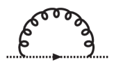
(G-a)

Figure 9: Diagram for the self-energy of the ghost. The curly line represents the propagator of $A_{i}$. The dotted line represents the propagator of the ghost.

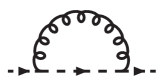
(F-a)

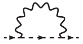
(F-b)

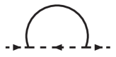
(F-c)

Figure 10: Diagrams for the one-loop self energy of $\psi^{A}$. The curly line represents the propagator of $A_{i}$. The wavy line represents the propagator of $A_{0}$. The solid line represents the propagator of $X_{AB}$. The dashed line represents the propagator of $\psi^{A}$.

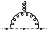
(GV-a)

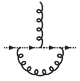
(GV-b)

Figure 11: Diagrams for the one-loop correction to the ghost-ghost-gauge interaction vertex. The curly line represents the propagator of $A_{i}$. The dotted line represents the propagator of the ghost.

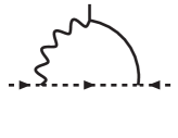
(Y-a)

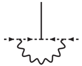
(Y-b)

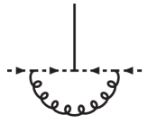
(Y-c)

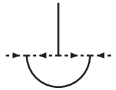
(Y-d)

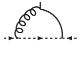
(Y-e)

Figure 12: Diagrams for the one-loop correction to the Yukawa interaction. The curly line represents the propagator of $A_{i}$. The wavy line represents the propagator of $A_{0}$. The solid line represents the propagator of $X_{AB}$. The dashed line represents the propagator of $\psi^{A}$.

In this appendix, we give the 1-loop diagrams and the divergent part of each diagram. The nine diagrams for the 1-loop self-energy of $A_{i}$ which is $(-i)$ times the 1-loop contribution to the 1PI part of the truncated 2-point function $\langle A_{JM\rho}(q)_{kl}A_{J^{\prime}M^{\prime}\rho^{\prime}}(-q)_{k^{\prime}l^{\prime}}\rangle$ are shown in Fig. 7. The six diagrams for the 1-loop self-energy of $A_{0}$ which is $(-i)$ times the 1-loop contribution to the 1PI part of the truncated 2-point function$\langle B_{JM}(q)_{kl}B_{J^{\prime}M^{\prime}}(-q)_{k^{\prime}l^{\prime}}\rangle$ are shown in Fig. 8. The diagram for the 1-loop self-energy of $c$ which is $(-i)$ times the 1-loop contribution to the 1PI part of the truncated 2-point function $\langle c_{JM}(q)_{kl}\bar{c}_{J^{\prime}M^{\prime}}(-q)_{k^{\prime}l^{\prime}}\rangle$ are shown in Fig. 9. The three diagram for the 1-loop self-energy of $\psi^{A}$ which is $(-i)$ times the 1-loop contribution to the 1PI part of the truncated 2-point function $\langle\psi_{JM\kappa}^{A}(q)_{kl}\psi_{J^{\prime}M^{\prime}\kappa^{\prime}A^{\prime}}^{\dagger}(q)_{kl^{\prime}}\rangle$ are shown in Fig. 10. The two diagrams for the 1-loop correction to the ghost-ghost-gauge interaction term which is $(-i)$ times the 1-loop contribution to the 1PI part of the truncated three point function $\langle A_{JM\rho}(q)_{kl}c_{J^{\prime}M^{\prime}}(q^{\prime})_{K^{\prime}l^{\prime}}\bar{c}_{J^{\prime\prime}M^{\prime\prime}}(q^{\prime\prime})_{k^{\prime\prime}l^{\prime\prime}}\rangle$ are shown in Fig. 11. The five diagrams for the one-loop correction to the Yukawa interaction term which is $(-i)$ times the 1-loop contribution to the 1PI part of the truncated three point function $\langle(X_{AB}^{JM}(q))_{kl}\psi_{J^{\prime}}^{A^{\prime}}(q^{\prime})_{k^{\prime}l^{\prime}}\psi_{J^{\prime\prime}}^{B^{\prime}}(q^{\prime\prime})_{k^{\prime\prime}l^{\prime\prime}}\rangle$, are shown in Fig. 12.

The 1-loop self-energy of $A_{i}$ takes the form

$$g^{2}N\delta_{kl^{\prime}}\delta_{lk^{\prime}}(-1)^{m-\tilde{m}+1}\delta_{JJ^{\prime}}\delta_{M-M^{\prime}}\delta_{\rho\rho^{\prime}}\Pi^{A}_{J}(q).$$ (D.1)

We list the the divergent part in the contribution of each diagram to $\Pi^{A}_{J}(q)$.

$$(A-a)=\sum_{J_{1},J_{2}\neq 0,M_{1}M_{2}}\frac{2i\delta(0)}{4\sqrt{J_{1}(J_{1}+1)J_{2}(J_{2}+1)}}\mathcal{D}_{J_{2}M_{2}\,J_{1}M_{1}0\,J-M\rho}\mathcal{D}_{J_{1}-M_{1}\,J_{2}-M_{2}0\,J^{\prime}-M^{\prime}\rho^{\prime}},$$

$$(A-b)=\sum_{J_{1},J_{2}\neq 0,M_{1}M_{2}}\bigg{[}-\frac{2i\delta(0)}{4\sqrt{J_{1}(J_{1}+1)J_{2}(J_{2}+1)}}\mathcal{D}_{J_{2}M_{2}\,J_{1}M_{1}0\,J-M\rho}\mathcal{D}_{J_{1}-M_{1}\,J_{2}-M_{2}0\,J^{\prime}-M^{\prime}\rho^{\prime}}$$

$$\qquad\qquad\;\;+\frac{2i\delta(0)}{4J_{2}(J_{2}+1)}\mathcal{D}_{J_{2}M_{2}\,J_{1}M_{1}0\,J-M\rho}\mathcal{D}_{J_{2}-M_{2}\,J_{1}-M_{1}0\,J^{\prime}-M^{\prime}\rho^{\prime}}\bigg{]},$$

$$(A-c)=\sum_{J_{2}\neq=0,J_{1}M_{1}M_{2}}\frac{-2i\delta(0)}{4J_{2}(J_{2}+1)}\bigg{[}\mathcal{D}_{J_{2}M_{2}\,J-M\rho\,J_{1}M_{1}0}\mathcal{D}_{J_{2}-M_{2}\,J^{\prime}-M^{\prime}\rho^{\prime}\,J_{1}-M_{1}0}$$

$$\qquad\qquad\;\;+\mathcal{D}_{J_{2}M_{2}\,J-M\rho\,J_{1}M_{1}\pm}\mathcal{D}_{J_{2}-M_{2}\,J^{\prime}-M^{\prime}\rho^{\prime}\,J_{1}-M_{1}\pm}\bigg{]},$$

$$(A-d)=\sum_{J_{2}\neq=0,J_{1}M_{1}M_{2}}\frac{2i\delta(0)}{4J_{2}(J_{2}+1)}\mathcal{D}_{J_{2}M_{2}\,J_{1}M_{1}\pm,J-M\rho}\mathcal{D}_{J_{2}-M_{2}\,J^{\prime}-M^{\prime}-\rho^{\prime}J_{5}M_{5}\pm}$$

$$\qquad\qquad\;\;-\frac{4}{3}\Lambda_{s}^{2}-2\Lambda_{s}-\left[\frac{2}{3}q^{2}+\frac{2}{5}(2J+2)^{2}+\frac{2}{5}\right]\log(2\Lambda),$$

$$(A-e)=-\frac{8}{3}\Lambda_{v}^{2}-\frac{20}{3}\Lambda_{v}+\frac{4}{3}\log(2\Lambda),$$

$$(A-f)=\frac{4}{3}\Lambda_{v}^{2}+\frac{10}{3}\Lambda_{v}+\left[\frac{q^{2}}{6}+\frac{18}{5}(J+1)^{2}-\frac{14}{15}\right]\log(2\Lambda),$$

$$(A-g)=-12\Lambda_{s}^{2}-18\Lambda_{s},$$

$$(A-h)=4\Lambda_{s}^{2}+6\Lambda_{s}+\frac{1}{2}\left[q^{2}-(2J+2)^{2}\right]\log(2\Lambda),$$

$$(A-i)=\frac{32}{3}\Lambda_{f}^{2}+\frac{64}{3}\Lambda_{f}+\frac{4}{3}\left[q^{2}-(2J+2)^{2}\right]\log(2\Lambda).$$ (D.2)

Note that the terms proportional to $\delta(0)$ cancel among $(A-a)\sim(A-d)$.

The 1-loop self-energy of $A_{0}$ takes the form

$$g^{2}N\delta_{kl^{\prime}}\delta_{lk^{\prime}}(-1)^{m-\tilde{m}}\delta_{JJ^{\prime}}\delta_{M-M^{\prime}}\Pi^{B}_{J}(q).$$ (D.3)

We list the the divergent part in the contribution of each diagram to $\Pi^{B}_{J}(q)$.

$$(B-a)=4\Lambda_{v}^{2}+10\Lambda_{v}-2\log(2\Lambda),$$

$$(B-b)=-4\Lambda_{v}^{2}-10\Lambda_{v}+\left[2+\frac{10}{3}J(J+1)\right]\log(2\Lambda),$$

$$(B-c)=-\frac{32}{3}J(J+1)\log(2\Lambda),$$

$$(B-d)=12\Lambda_{s}^{2}+18\Lambda_{s},$$

$$(B-e)=-12\Lambda_{s}^{2}-18\Lambda_{s}+2J(J+1)\log(2\Lambda),$$

$$(B-f)=\frac{16}{3}J(J+1)\log(2\Lambda).$$ (D.4)

The 1-loop self-energy of $c$ takes the form

$$g^{2}N\delta_{kl^{\prime}}\delta_{lk^{\prime}}(-1)^{m-\tilde{m}}\delta_{JJ^{\prime}}\delta_{M-M^{\prime}}\Pi^{c}_{J}(q).$$ (D.5)

The divergent part in the contribution of the diagram to $\Pi^{c}_{J}(q)$ is

$$(G-a)=4iJ(J+1)\left(-\frac{2}{3}\right)\log(2\Lambda).$$ (D.6)

The 1-loop self-energy of $\psi^{A}$ takes the form

$$g^{2}N\delta_{kl^{\prime}}\delta_{lk^{\prime}}\delta_{JJ^{\prime}}\delta_{MM^{\prime}}\delta_{\kappa\kappa^{\prime}}\delta^{A}_{A^{\prime}}\Pi^{\psi}_{J}(q).$$ (D.7)

We list the the divergent part in the contribution of each diagram to $\Pi^{\psi}_{J}(q)$.

$$(F-a)=\left(\frac{1}{2}q-\frac{1}{6}\kappa(2J+\frac{3}{2})\right)\log(2\Lambda),$$

$$(F-b)=\left(\frac{2}{3}\kappa(2J+\frac{3}{2})\right)\log(2\Lambda),$$

$$(F-c)=\frac{3}{2}\left(q+\kappa(2J+\frac{3}{2})\right)\log(2\Lambda).$$ (D.8)

The two diagrams for the one-loop correction to the ghost-ghost-gauge interaction term vanish:

$$(GV-a)=0,\;\;\;\;\;(GV-b)=0.$$ (D.9)

The 1-loop correction to the Yukawa interaction term takes the form

$$2ig^{3}N\delta_{AB}^{A^{\prime}B^{\prime}}\left(\delta_{kl^{\prime}}\delta_{k^{\prime}l^{\prime\prime}}\delta_{k^{\prime\prime}l}(-1)^{m^{\prime}-\tilde{m}^{\prime}+\frac{\kappa^{\prime}}{2}}F^{J^{\prime\prime}M^{\prime\prime}\kappa^{\prime\prime}}_{J^{\prime}-M^{\prime}\kappa^{\prime}\;J_{3}-M_{3}}+\delta_{kl^{\prime\prime}}\delta_{k^{\prime}l}\delta_{k^{\prime\prime}l^{\prime}}(-1)^{m^{\prime\prime}-\tilde{m}^{\prime\prime}+\frac{\kappa^{\prime\prime}}{2}}F^{J^{\prime}M^{\prime}\kappa^{\prime}}_{J^{\prime\prime}-M^{\prime\prime}\kappa^{\prime\prime}\;J_{3}-M_{3}}\right)$$

$$\times 2\pi\delta(q+q^{\prime}+q^{\prime\prime})\Gamma^{Y}_{JJ^{\prime}J^{\prime\prime}}(q^{\prime},q^{\prime\prime}).$$ (D.10)

We list the the divergent part in the contribution of each diagram to $\Gamma^{Y}_{JJ^{\prime}J^{\prime\prime}}(q^{\prime},q^{\prime\prime})$.

$$(Y-a)=\frac{1}{2}\log(2\Lambda),$$

$$(Y-b)=\frac{1}{2}\log(2\Lambda),$$

$$(Y-c)=\frac{1}{2}\log(2\Lambda),$$

$$(Y-d)=\log(2\Lambda),$$

$$(Y-e)=0.$$ (D.11)

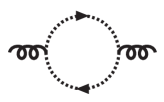
(A-a)

(A-b)

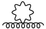
(A-c)

(A-d)

(A-e)

(A-f)

(A-g)

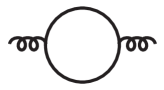
(A-h)

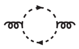
(A-i)

Figure 7: Diagrams for the one-loop self energy of $A_{i}$. The curly line represents the propagator of $A_{i}$. The wavy line represents the propagator of $A_{0}$. The dotted line represents the propagator of the ghost. The solid line represents the propagator of $X_{AB}$. The dashed line represents the propagator of $\psi^{A}$.

Appendix E 1-loop effective action in the truncated theories

In this appendix, we give the expressions for the 1-loop effective action around the time-dependent BPS solution in the truncated theories. In the expressions, we omit the factor $g^{2}N\int dt$ to make them compact.

The 1-loop effective action in the plane-wave matrix model is

$$\Gamma_{eff}^{Z0}=-\sqrt{4+l},$$

$$\Gamma_{eff}^{Y}=-4\sqrt{1+l},$$

$$\Gamma_{eff}^{A}=-3\sqrt{4+l},$$

$$\Gamma_{eff}^{F}=4(\sqrt{4+l}+\sqrt{1+l}\>).$$ (E.1)

The 1-loop effective action in ${\cal N}=4$ SYM on $R\times S^{2}$ is

$$\Gamma_{eff}^{Z0}=-\sqrt{4+l},$$

$$\Gamma_{eff}^{Z}=-\sum_{J\in\mathbf{Z}_{>0}}(2J+1)(\sqrt{4J^{2}+l}+\sqrt{(2J+2)^{2}+l}\>),$$

$$\Gamma_{eff}^{Y}=-4\sum_{J\in\mathbf{Z}_{\geq 0}}(2J+1)\sqrt{(2J+1)^{2}+l},$$

$$\Gamma_{eff}^{A}=-\sum_{J\in\mathbf{Z}_{\geq 0}}((2J+3)\sqrt{(2J+2)^{2}+l}+(2J+1)\sqrt{(2J+2)^{2}+l}\>),$$

$$\Gamma_{eff}^{F}=2\sum_{J\in\mathbf{Z}_{\geq 0}}(2J+2)(\sqrt{(2J+2)^{2}+l}+\sqrt{(2J+1)^{2}+l}\>)$$

$$\qquad\quad\;+2\sum_{J\in\frac{1}{2}+\mathbf{Z}_{\geq 0}}(2J+1)(\sqrt{(2J+2)^{2}+l}+\sqrt{(2J+1)^{2}+l}\>),$$

$$\Gamma_{eff}^{c.t.}=-\frac{g^{2}Nl}{2}\left(\Pi_{J=0}^{X}(1)+\frac{1}{2}\right).$$ (E.2)

The 1-loop effective action in ${\cal N}=4$ SYM on $R\times S^{3}/Z_{k}$ with $k$ even is

$$\Gamma_{eff}^{Z0}=-\sqrt{4+l},$$

$$\Gamma_{eff}^{Z}=-\left(\sum_{n\in\mathbf{Z}_{>0}}\sum_{v=0}^{\frac{k}{2}-1}+\left.\sum_{v=1}^{\frac{k}{2}-1}\right|_{n=0}\right)$$

$$\qquad\qquad\;\;(kn+2v+1)(2n+1)(\sqrt{(kn+2v)^{2}+l}+\sqrt{(kn+2v+2)^{2}+l}\>),$$

$$\Gamma_{eff}^{Y}=-4\sum_{n\in\mathbf{Z}_{\geq 0}}\sum_{v=0}^{\frac{k}{2}-1}(kn+2v+1)(2n+1)\sqrt{(kn+2v+1)^{2}+l},$$

$$\Gamma_{eff}^{A}=-\sum_{n\in\mathbf{Z}_{\geq 0}}\sum_{v=0}^{\frac{k}{2}-1}(kn+2v+3)(2n+1)\sqrt{(kn+2v+2)^{2}+l}$$

$$\qquad\quad\;-\left(\sum_{n\in\mathbf{Z}_{>0}}\sum_{v=0}^{\frac{k}{2}-1}+\left.\sum_{v=1}^{\frac{k}{2}-1}\right|_{n=0}\right)(kn+2v-1)(2n+1)\sqrt{(kn+2v)^{2}+l},$$

$$\Gamma_{eff}^{F}=2\sum_{n\in\mathbf{Z}_{\geq 0}}\sum_{v=0}^{\frac{k}{2}-1}(kn+2v+2)(2n+1)(\sqrt{(kn+2v+2)^{2}+l}+\sqrt{(kn+2v+1)^{2}+l}\>)$$

$$\qquad\;\;\;+2\left(\sum_{n\in\mathbf{Z}_{>0}}\sum_{v=0}^{\frac{k}{2}-1}+\left.\sum_{v=1}^{\frac{k}{2}-1}\right|_{n=0}\right)(kn+2v)(2n+1)(\sqrt{(kn+2v+1)^{2}+l}+\sqrt{(kn+2v)^{2}+l}\>),$$

$$\Gamma_{eff}^{c.t.}=-\frac{g^{2}Nl}{2}\left(\Pi_{J=0}^{X}(1)+\frac{1}{2}\right).$$ (E.3)

The 1-loop effective action in ${\cal N}=4$ SYM on $R\times S^{3}/Z_{k}$ with $k$ odd is

$$\Gamma_{eff}^{Z0}=-\sqrt{4+l},$$

$$\Gamma_{eff}^{Z}=-\left(\sum_{n\in\mathbf{Z}_{>0}}\sum_{v=0}^{\frac{k}{2}-\frac{1}{2}}+\left.\sum_{v=1}^{\frac{k}{2}-\frac{1}{2}}\right|_{n=0}\right)$$

$$\qquad\qquad\;\;(kn+2v+1)(n+1)(\sqrt{(kn+2v)^{2}+l}+\sqrt{(kn+2v+2)^{2}+l}\>)$$

$$\qquad\quad-\sum_{n\in\mathbf{Z}_{\geq 0}}\sum_{v=1}^{\frac{k}{2}-\frac{1}{2}}(kn+2v)n(\sqrt{(kn+2v-1)^{2}+l}+\sqrt{(kn+2v+1)^{2}+l}\>),$$

$$\Gamma_{eff}^{Y}=-4\sum_{n\in\mathbf{Z}_{\geq 0}}\sum_{v=0}^{\frac{k}{2}-\frac{1}{2}}(kn+2v+1)(n+1)\sqrt{(kn+2v+1)^{2}+l}$$

$$\qquad\quad-4\sum_{n\in\mathbf{Z}_{\geq 0}}\sum_{v=1}^{\frac{k}{2}-\frac{1}{2}}(kn+2v)n\sqrt{(kn+2v)^{2}+l},$$

$$\Gamma_{eff}^{A}=-\sum_{n\in\mathbf{Z}_{\geq 0}}\sum_{v=0}^{\frac{k}{2}-\frac{1}{2}}(kn+2v+3)(n+1)\sqrt{(kn+2v+2)^{2}+l}$$

$$\qquad\quad-\left(\sum_{n\in\mathbf{Z}_{>0}}\sum_{v=0}^{\frac{k}{2}-\frac{1}{2}}+\left.\sum_{v=1}^{\frac{k}{2}-\frac{1}{2}}\right|_{n=0}\right)(kn+2v-1)(n+1)\sqrt{(kn+2v)^{2}+l}$$

$$\qquad\;\;\;-\sum_{n\in\mathbf{Z}_{\geq 0}}\sum_{v=1}^{\frac{k}{2}-\frac{1}{2}}((kn+2v+2)n\sqrt{(kn+2v+1)^{2}+l}+(kn+2v-2)n\sqrt{(kn+2v-1)^{2}+l}\>),$$

$$\Gamma_{eff}^{F}=2\sum_{n\in\mathbf{Z}_{\geq 0}}\sum_{v=0}^{\frac{k}{2}-\frac{1}{2}}(kn+2v+2)(n+1)(\sqrt{(kn+2v+2)^{2}+l}+\sqrt{(kn+2v+1)^{2}+l}\>)$$

$$\qquad\quad+2\left(\sum_{n\in\mathbf{Z}_{>0}}\sum_{v=0}^{\frac{k}{2}-\frac{1}{2}}+\left.\sum_{v=1}^{\frac{k}{2}-\frac{1}{2}}\right|_{n=0}\right)(kn+2v)(n+1)(\sqrt{(kn+2v+1)^{2}+l}+\sqrt{(kn+2v)^{2}+l}\>)$$

$$\qquad\quad+2\sum_{n\in\mathbf{Z}_{\geq 0}}\sum_{v=1}^{\frac{k}{2}-\frac{1}{2}}((kn+2v+1)n(\sqrt{(kn+2v+1)^{2}+l}+\sqrt{(kn+2v)^{2}+l}\>)$$

$$\qquad\qquad\qquad\qquad+(kn+2v-1)n(\sqrt{(kn+2v)^{2}+l}+\sqrt{(kn+2v-1)^{2}+l}\>)),$$

$$\Gamma_{eff}^{c.t.}=-\frac{g^{2}Nl}{2}\left(\Pi_{J=0}^{X}(1)+\frac{1}{2}\right).$$ (E.4)

References

- [1] H. Lin and J. Maldacena, “Fivebranes from gauge theory,” arXiv:hep-th/0509235.
- [2] H. Lin, O. Lunin and J. Maldacena, “Bubbling AdS space and 1/2 BPS geometries,” JHEP 0410 (2004) 025 [arXiv:hep-th/0409174].
- [3] S. Corley, A. Jevicki and S. Ramgoolam, “Exact correlators of giant gravitons from dual N = 4 SYM theory,” Adv. Theor. Math. Phys. 5 (2002) 809 [arXiv:hep-th/0111222].
- [4] D. Berenstein, “A toy model for the AdS/CFT correspondence,” JHEP 0407 (2004) 018 [arXiv:hep-th/0403110].
- [5] D. Berenstein, J. M. Maldacena and H. Nastase, “Strings in flat space and pp waves from N = 4 super Yang Mills,” JHEP 0204 (2002) 013 [arXiv:hep-th/0202021].
- [6] J. Maldacena, M. M. Sheikh-Jabbari and M. Van Raamsdonk, “Transverse fivebranes in matrix theory,” JHEP 0301 (2003) 038 [arXiv:hep-th/0211139].
- [7] K. Dasgupta, M. M. Sheikh-Jabbari and M. Van Raamsdonk, “Protected multiplets of M-theory on a plane wave,” JHEP 0209 (2002) 021 [arXiv:hep-th/0207050].
- [8] K. Dasgupta, M. M. Sheikh-Jabbari and M. Van Raamsdonk, “Matrix perturbation theory for M-theory on a PP-wave,” JHEP 0205 (2002) 056 [arXiv:hep-th/0205185].
- [9] N. w. Kim and J. Plefka, “On the spectrum of pp-wave matrix theory,” Nucl. Phys. B 643, 31 (2002) [arXiv:hep-th/0207034].
- [10] N. w. Kim, T. Klose and J. Plefka, “Plane-wave matrix theory from N = 4 super Yang-Mills on R x S**3,” Nucl. Phys. B 671, 359 (2003) [arXiv:hep-th/0306054].
- [11] T. Klose and J. Plefka, “On the integrability of large N plane-wave matrix theory,” Nucl. Phys. B 679, 127 (2004) [arXiv:hep-th/0310232].
- [12] T. Fischbacher, T. Klose and J. Plefka, “Planar plane-wave matrix theory at the four loop order: Integrability without BMN scaling,” JHEP 0502, 039 (2005) [arXiv:hep-th/0412331].
- [13] N. Beisert and T. Klose, “Long-range gl(n) integrable spin chains and plane-wave matrix theory,” arXiv:hep-th/0510124.
- [14] P. Breitenlohner and D. Z. Freedman, “Stability In Gauged Extended Supergravity,” Annals Phys. 144 (1982) 249.
- [15] H. Nicolai, E. Sezgin and Y. Tanii, “Conformally Invariant Supersymmetric Field Theories On S**P X S**1 And Super P-Branes,” Nucl. Phys. B 305 (1988) 483.
- [16] E. Bergshoeff, A. Salam, E. Sezgin and Y. Tanii, “N=8 Supersingleton Quantum Field Theory,” Nucl. Phys. B 305 (1988) 497.
- [17] K. Okuyama, “N = 4 SYM on R x S(3) and pp-wave,” JHEP 0211, 043 (2002) [arXiv:hep-th/0207067].
- [18] A. Hashimoto, S. Hirano and N. Itzhaki, “Large branes in AdS and their field theory dual,” JHEP 0008 (2000) 051 [arXiv:hep-th/0008016].
- [19] E. Witten, “Anti-de Sitter space, thermal phase transition, and confinement in gauge theories,” Adv. Theor. Math. Phys. 2 (1998) 505 [arXiv:hep-th/9803131].
- [20] B. Sundborg, “The Hagedorn transition, deconfinement and N = 4 SYM theory,” Nucl. Phys. B 573 (2000) 349 [arXiv:hep-th/9908001].
- [21] O. Aharony, J. Marsano, S. Minwalla, K. Papadodimas and M. Van Raamsdonk, “The Hagedorn / deconfinement phase transition in weakly coupled large N gauge theories,” Adv. Theor. Math. Phys. 8 (2004) 603 [arXiv:hep-th/0310285].
- [22] S.W. Hawking and D.N. Page, “Thermodynamics of black holes in anti-de Sitter Space,” Comm. Math. Phys. 87 (1983) 577.
- [23] See for example: A. Cappelli and A. Coste, “On The Stress Tensor Of Conformal Field Theories In Higher Dimensions,” Nucl. Phys. B 314, 707 (1989).
- [24] E. Bergshoeff, M. J. Duff, C. N. Pope and E. Sezgin, “Supersymmetric Supermembrane Vacua And Singletons,” Phys. Lett. B 199 (1987) 69.
- [25] A. Salam and J. A. Strathdee, “On Kaluza-Klein Theory,” Ann. Phys. 141, 316 (1982).
- [26] R. E. Cutkosky, “Harmonic Functions And Matrix Elements For Hyperspherical Quantum Field Models,” J. Math. Phys. 25 (1984) 939.
- [27] K. j. Hamada and S. Horata, “Conformal algebra and physical states in non-critical 3-brane on R x S**3,” Prog. Theor. Phys. 110, 1169 (2004) [arXiv:hep-th/0307008].
- [28] O. Aharony, J. Marsano, S. Minwalla, K. Papadodimas and M. Van Raamsdonk, “A first order deconfinement transition in large N Yang-Mills theory on a small S**3,” Phys. Rev. D 71, 125018 (2005) [arXiv:hep-th/0502149].
- [29] S. Deger, A. Kaya, E. Sezgin and P. Sundell, “Spectrum of D = 6, N = 4b supergravity on AdS(3) x S(3),” Nucl. Phys. B 536 (1998) 110 [arXiv:hep-th/9804166].
- [30] J. A. Minahan and K. Zarembo, “The Bethe-ansatz for N = 4 super Yang-Mills,” JHEP 0303, 013 (2003) [arXiv:hep-th/0212208].
- [31] G. ’t Hooft, “Renormalization of massless Yang-Mills fields,” Nucl. Phys. B33 (1971) 173.
- [32] D. Varshalovich, A. Moskalev and V. Khersonskii, Quantum Theory of Angular Momentum (World Scientific, Singapore, 1988).
- [33] N. Beisert, C. Kristjansen and M. Staudacher, Nucl. Phys. B 664 (2003) 131 [arXiv:hep-th/0303060].
- [34] H. Shin and K. Yoshida, “One-loop flatness of membrane fuzzy sphere interaction in plane-wave matrix model,” Nucl. Phys. B 679, 99 (2004) [arXiv:hep-th/0309258].
- [35] H. Shin and K. Yoshida, “Membrane fuzzy sphere dynamics in plane-wave matrix model,” Nucl. Phys. B 709, 69 (2005) [arXiv:hep-th/0409045].
- [36] H. Shin and K. Yoshida, “Point-like graviton scattering in plane-wave matrix model,” arXiv:hep-th/0511072.
- [37] N. Kawahara, J. Nishimura and K. Yoshida, “Dynamical aspects of the plane-wave matrix model at finite temperature,” arXiv:hep-th/0601170.
- [38] D. Yamada and L. G. Yaffe, “Phase Diagram of Super-Yang-Mills Theory with -Symmetry Chemical Potentials,” hep-th/0602074.
- [39] L. Alvarez-Gaume, P. Basu, M. Marino and S. R. Wadia, “Blackhole / string transition for the small Schwarzschild blackhole of and critical unitary matrix models,” hep-th/0605041.