Close to the edge: hierarchy in a double braneworld

Abstract

We show that the hierarchy between the Planck and the weak scales can follow from the tendency of gravitons and fermions to localize at different edges of a thick double wall embedded in an $AdS_{5}$ spacetime without reflection symmetry. This double wall is a stable BPS thick-wall solution with two sub-walls located at its edges; fermions are coupled to the scalar field through Yukawa interactions, but the lack of reflection symmetry forces them to be localized in one of the sub-walls. We show that the graviton zero-mode wavefunction is suppressed in the fermion edge by an exponential function of the distance between the sub-walls, and that the massive modes decouple so that Newtonian gravity is recuperated.

I Introduction

The idea of confining our four-dimensional Universe inside a topological defect embedded in a higher dimensional spacetime dates at least as far back as the suggestion of Rubakov and Shaposhnikov Rubakov:1983bb (see also Akama:1982jy ) that we could be living inside a domain wall. They showed that fermions (of one chirality) can be confined to the wall by their Yukawa interactions with the scalar field. Domain walls are vacuum configurations that are topologically protected and thus stable, but their gravitational interactions cannot be ignored. This became evident after the work of Randall and Sundrum Randall:1999vf , in which they showed that the five-dimensional metric produced by an infinitely thin brane is enough to ensure that Newtonian gravity is reproduced on the brane.

Actually, the RS brane does not even have to be a true domain wall, in the sense that no scalar field is needed for the effect. One just has to ensure that the bulk spacetime is Anti-De Sitter (AdS), and on the brane the four-dimensional cosmological constant is set to zero. The natural question is then whether fermions can also benefit from this effect, allowing us to live in a domain wall just because of its self-gravitation. The answer is on the negative, as shown in Bajc:1999mh fermion modes behave exactly opposite as the gravitons, the warp factor forcing them to escape from the wall into the bulk. If one wants matter to be confined to the wall, it is necessary to combine Rubakov-Shaposhnikov with Randall-Sundrum, i.e., to consider a real domain wall, made up of the vacuum expectation value of a scalar field that breaks a discrete symmetry, take into account its gravitational self-interactions, and make it couple to the fermions. This amounts to solve the five-dimensional coupled Einstein-Klein-Gordon system for an adequate potential, and many such solutions can be found in the literature. Among them, BPS walls, those where the four-dimensional cosmological constant is set to zero, are the most appealing “thick brane” generalizations of the Randall-Sundrum scenario. BPS solutions to the Einstein-Klein-Gordon system can be found by means of an auxiliary function of the scalar field, the fake superpotential of the first-order formalism of Behrndt:1999kz ; Skenderis:1999mm ; DeWolfe:1999cp .

The fact that fermion zero mode localization requires exactly the inverse warp factor as graviton zero mode localization, is used in this paper to provide a rationale for the large hierarchy between the Planck and weak scales in some particular thick wall solutions. These solutions are a straightforward generalization of the simplest BPS wall which represents a smoothing of the scenario of Randall:1999vf , found by Gremm Gremm:1999pj . The generalization produces an asymmetric double wall system: a BPS wall with a substructure consisting of two sub-wall located at its edges, but with different bulk cosmological constants on both sides. As a consequence of the asymmetry, fermions coupled to the scalar field are forced by the warp factor to localize on one of the sub-walls, the fermion sub-wall. On the other hand, the graviton zero-mode wavefunction is suppressed in the fermion sub-wall by an exponential function of the wall’s thickness, i.e. the distance between the sub-walls, and gravitons localize in the opposite sub-wall, the Planck sub-wall. This allows one to provide a large hierarchy between the effective Planck masses on both sub-walls, as proposed by Randall and Sundrum in their earlier work Randall:1999ee but with no orbifold geometries and no negative tension branes.

Attempts to achieve suppressed mass scales with two positive tension branes, the so-called Lykken-Randall scenario Lykken:1999nb , are found in the literature losotros . To our knowledge, however, all of them require some form of radion field in order to stabilize the extra dimension Kanti:2002zr . In our case, the stability of the two wall system stems from their topological properties, they are just a special kind of BPS walls. The fact that no compactification of the bulk coordinate is required allows us to reproduce Newtonian gravity on the walls as in Randall:1999vf , while keeping a large mass hierarchy as in Randall:1999ee . Moreover, the fermions are not arbitrarily assumed to be located in a different wall as the gravitons, they do so as a consequence of spacetime being warped. In contrast with the scenario of Lykken:1999nb , the fermion sub-wall is not a “probe” brane, and it has a non-negligible tension.

The paper is organized as follows. In the next Section we give an overview of the mechanism that provides stable, asymmetric double walls from a known BPS solution, and how fermions get localized on the brane with larger Planck mass. The following section is dedicated to explicitly construct these solutions from the simplest known BPS wall of Gremm:1999pj , to find the graviton and fermion zero modes, and to calculate the Newtonian potential.

II Double walls and hierarchy

The so-called BPS double walls are solutions to the 5-dimensional Einstein-scalar field set of equations that satisfy the BPS condition. As such, for the line element written in “proper length” coordinates

$$ds^{2}=e^{2A(\xi)}\eta_{\mu\nu}dx^{\mu}dx^{\nu}+d\xi^{2}$$ (1)

they can be generated from a “fake superpotential” $W(\phi)$ Behrndt:1999kz ; Skenderis:1999mm ; DeWolfe:1999cp by solving the BPS equations for the scalar field, warp factor and scalar potential

$$\phi^{\prime} = 3\frac{dW}{d\phi}$$

$$A^{\prime} = -W$$

$$V(\phi) = \frac{3}{2}\left[3\left(\frac{dW}{d\phi}\right)^{2}-4W^{2}\right]$$ (2)

where prime denotes derivative with respect to the bulk coordinate $\xi$. For $W(\phi)$ given by

$$W(\phi)=\alpha[\sin(\phi/\phi_{0})]^{2-1/s},$$ (3)

with $\alpha$ and $\phi_{0}$ real constants, solutions to (2) were found in Melfo:2002wd representing a family of double branes parametrized by an odd integer $s>1$ that interpolate between $AdS_{5}$ spacetimes. For $s=1$, this is just the brane of Ref. Gremm:1999pj , i.e. a regularization of the infinitely-thin RS brane, but for $s>1$ the wall splits in two in a well defined sense: the energy density has two maxima as can be seen in Fig. 1. The fact that exponentiating the superpotential for a single wall gives rise to double systems was also used in CBazeia:2003qt to construct BPS double walls. The topological charge is given by the asymptotic values of the superpotential

$$Q_{T}=W(+\infty)-W(-\infty)=2\alpha$$ (4)

and is independent of $s$, i.e., it is the same as in the single wall.

We have then a stable wall with two sub-walls, in which the thickness of the sub-walls goes to zero as $s\rightarrow\infty$, while the separation between them remains fixed. The spacetime far away of the wall is $AdS_{5}$ with the same cosmological constant ($\Lambda_{\pm}$) on both sides, while the spacetime in between the sub-branes is nearly flat, i.e.

$$\Lambda_{\pm}=-6\alpha^{2},\qquad\Lambda_{\rm in}=0$$ (5)

The gravitational zero modes are calculated as usual

$$\psi^{g}_{0}=N_{g}\,e^{2A(\xi)}$$ (6)

with $N_{g}$ a normalization factor. Because the spacetime between the two sub-branes is nearly flat, the zero modes are not peaked at $\xi=0$, but instead distribute smoothly over the whole system Castillo-Felisola:2004eg , as seen in Fig. 1. A similar behavior has been found for other BPS double branes CBazeia:2003qt .

Fermion modes of a given chirality can also be localized, by adding as usual a Yukawa coupling $\lambda$ with the scalar field Bajc:1999mh . One obtains

$$\psi_{0}^{f}(\xi)\sim\,e^{-2A(\xi)}e^{-\lambda\int\phi(\xi)d\xi}$$ (7)

The fermion zero modes for the system considered have been calculated in Melfo:2006hh , and can be seen in Fig. 1. Details of the calculation are given in the next section, but the general behavior will suffice for the time being.

Now, suppose the superpotential is shifted by a positive constant

$$\tilde{W}=W+\beta$$ (8)

According to (2), we will have the same solution for the scalar field. Furthermore, since for the double wall (2,3), the extrema of $V(\phi)$ are the same ones of $W(\phi)$, it follows that the extrema of the new scalar potential $\tilde{V}(\phi)$ are the same ones of $V(\phi)$, namely $\phi=0$ and $\phi=\pm\pi\phi_{0}/2$. Hence, the two sub-walls are situated at the same place as before. Notice that the topological charge is the same. However, the cosmological constants are now different at the two sides of the double wall and the spacetime in between the sub-walls is no longer flat, one has

$$\Lambda_{-}=-6(\alpha-\beta)^{2},\quad\Lambda_{+}=-6(\alpha+\beta)^{2},\quad\Lambda_{\rm in}=-6\beta^{2}$$ (9)

Accordingly, the new warp factor is from (2)

$$\tilde{A}(\xi)=A(\xi)-\beta\xi$$ (10)

As long as we keep $\beta<\alpha$, the gravitational zero modes remain localized, but now they are exponentially suppressed for $\xi>0$

$$\tilde{\psi}_{0}^{g}\sim\,\psi_{0}^{g}\,e^{-2\beta\xi}$$ (11)

so that the graviton zero-mode function gets shifted towards the region with a smaller cosmological constant, i.e. with $\Lambda_{-}$.

Fermion modes behave in exactly the opposite way, they are now

$$\tilde{\psi}^{f}_{0}\sim\,\psi^{f}_{0}\,e^{2\beta\xi}$$ (12)

so that they are shifted towards the larger cosmological constant region, i.e. with $\Lambda_{+}$. In other words, the gravitons are localized on the sub-brane situated at $\xi_{-}$, henceforth the Planck brane, while the fermion zero modes do the opposite, they live in the opposite sub-brane around $\xi_{+}$, the weak brane. The situation is depicted in Fig. 2.

The Planck masses in the Planck brane, $M_{Pl}^{\rm Planck}$, and in the weak brane, $M_{Pl}^{\rm Weak}$, are approximately related by

$$M_{Pl}^{\rm Planck}=M_{Pl}^{\rm Weak}e^{-2\beta\Delta}$$ (13)

with $\Delta$ the inter-sub-brane separation. Since $\Delta$ here is a coordinate-dependent quantity, Eq.(13) should be made precise by calculating and comparing the gravitational potential on both sub-branes, which we do in the next section.

As the thickness of the sub-branes approaches zero, this solution amounts to having a thick domain wall with two infinitely-thin sub-branes, the Planck brane and the weak brane, situated at different edges (in the transverse direction) of the wall. Clearly, the crucial role here is played by the double-brane solution, for which BPS stability arguments apply Skenderis:1999mm .

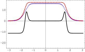
Figure 1: Energy density (continuous), gravitational zero mode (dashed) and fermion zero mode (dotted) for the double branes with $\alpha>0,\beta=0,\delta=4,s=11,\lambda=4\alpha$, and arbitrary normalization.

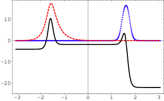
Figure 2: Energy density (continuous), gravitational zero mode (dashed) and fermion zero mode (dotted) for the double branes with $\alpha>0,\beta=0.8\alpha,\delta=4,s=11,\lambda=4\alpha$, and arbitrary normalization.

III Explicit solutions

III.1 Double branes

Solutions to the system (2) with un-shifted superpotential (3) (i.e. reflection symmetry) have been found in Melfo:2002wd by switching to the so-called “gauge” coordinates, where the metric is written as

$$ds^{2}=e^{2A(y)}\eta_{\mu\nu}dx^{\mu}dx^{\nu}+e^{2H(y)}dy^{2}$$ (14)

The field equations can be integrated to give

$$H(y) = -\frac{1}{2s}\ln\left[1+\left(\frac{\alpha y}{\delta}\right)^{2s}\right],\qquad A(y)=\delta H(y)$$

$$V(\phi) = 3\alpha^{2}[\sin(\phi/\phi_{0})]^{2-2/s}\left[\frac{2s+4\delta-1}{2\delta}\cos^{2}(\phi/\phi_{0})-2\right]$$

$$\phi(y) = \phi_{0}\arctan\left(\frac{\alpha y}{\delta}\right)^{s},\quad\phi_{0}=\frac{\sqrt{3\delta(2s-1)}}{s}$$ (15)

The parameter $\delta$ gives the thickness of the wall. For $s=1$, this is just the brane of Ref. Gremm:1999pj and it can be rigorously shown that the distributional limit $\delta\to 0$ gives the RS spacetime Guerrero:2002ki . But for non-zero $\delta$ and $s>1$, the energy density has two maxima, as can be seen in Fig. 1. Other double wall systems have been found in CBazeia:2003qt and Guerrero:2005aw .

These walls have been studied in detail in a series of papers, their thin wall limit $\delta\rightarrow 0$ in Melfo:2002wd , localization of gravity in Castillo-Felisola:2004eg and of chiral fermion modes in Melfo:2006hh . For $\delta=1$, there is a normalizable zero mode and a continuous of massive states that asymptote to plane waves as $y\rightarrow\pm\infty$. This continuum of modes decouple, in the sense that they generate small corrections to the Newtonian potential of the wall, at scales larger than the fundamental length-scale of the system, $\alpha^{-1}$.

Let us consider the double domain wall (14, III.1) for $s\gg 1$. The separation between the sub-branes, i.e. the distance between the maxima of the energy density, is given by

$$\Delta=2\frac{\delta}{\alpha}\left(\frac{s-1}{s+2\delta}\right)^{1/{2s}}$$ (16)

which behaves as $2{\delta}/{\alpha}$ for $s\gg 1$, while their thickness $\gamma$ is approximately given by

$$\gamma\sim\frac{1}{\alpha}\frac{\delta}{s}\ln\left(\frac{s}{\delta}\right)+O(s^{-2})$$ (17)

from which follows that $\gamma\sim 0$ for $s\gg 1$. Note that the double wall is lost in the $\delta\rightarrow 0$ limit Melfo:2002wd , as expected from the fact that the distributional geometry $\delta\rightarrow 0$ may be identified with the asymptotic behavior (i.e. far away from the wall) of the domain wall spacetime Pantoja:2003zr .

Following Guerrero:2002ki , the distributional limit $s\to\infty$ of the Einstein tensor is found to be

$$\lim_{s\rightarrow\infty}\left(G^{a}_{\,\,b}+\Lambda g^{a}_{\,\,b}\right)=$$

$$-3\alpha\left[\delta(y-y_{+})+\delta(y-y_{-})\right]\left(\partial^{a}dt_{b}+\partial^{b}_{x^{i}}dx^{i}_{b}\right)$$ (18)

with $\Lambda$ given by

$$-\frac{\Lambda}{6}=\begin{cases}\alpha^{2},&|y|>\delta/\alpha\cr 0,&|y|<\delta/\alpha\cr\end{cases}$$ (19)

Hence for $s\gg 1$ we have two infinitely thin walls located at $y_{+}=\delta/\alpha$ and $y_{-}=-\delta/\alpha$, with tensions $\sigma_{+}=\sigma_{-}=3\alpha>0$. On the other hand, we find that the limit ${s\rightarrow\infty}$ of the metric tensor gives the line element

$$ds^{2}=\left\{\begin{array}[]{lr}\left(\frac{\delta}{\alpha y}\right)^{2\delta}(-dt^{2}+dx^{i}dx^{i})+\left(\frac{\delta}{\alpha y}\right)^{2}dy^{2}&,|y|>{\delta}/{\alpha}\\ &\\ -dt^{2}+dx^{i}dx^{i}+dy^{2}&,|y|<\delta/\alpha\end{array}\right.$$ (20)

and the distributional Einstein tensor (III.1) turns out to be the Einstein tensor of the limit metric (20).

III.2 Asymmetric double branes

Now, shifting the superpotential as in (8) results in a solution with

$$\tilde{H}(y) = H(y)$$

$$\tilde{A}(y) = A(y)-\beta y\mathcal{F}(y)$$

$$\tilde{V}(\phi) = V(\phi)-6\beta[\beta+2\alpha(\sin(\phi/\phi_{0}))^{2-1/s}]$$

$$\tilde{\phi}(y) = \phi(y)$$ (21)

where $\mathcal{F}(y)\equiv\,_{2}F_{1}[1/2s,1/2s,1+1/2s,-(\alpha y/\delta)^{2s}]$ is the hypergeometric function. For $|\alpha y/\delta|\leq 1$, i.e. inside the double brane, and large $s$, ${}_{2}F_{1}\,\sim 1$ is a very good approximation, although we have used the exact solution whenever performing numerical integrations.

The equation for the gravitational zero modes is found as usual. In the axial gauge $h_{\mu y}=0$, writing the transverse-traceless part of the metric perturbations $h_{\mu\nu}$ as

$$h_{\mu\nu}=e^{ip\cdot x}e^{H/2}\psi_{\mu\nu}$$ (22)

one obtains

$$\left(-\frac{d^{2}}{dy^{2}}+U(y)\right)\psi_{\mu\nu}=m^{2}e^{-2\tilde{A}+2H}\psi_{\mu\nu}$$ (23)

with

$$U(y)=e^{-2\tilde{A}+H/2}(e^{2\tilde{A}-H/2})^{\prime\prime}$$ (24)

As usual, in order to get a Schrödinger-like equation, one must change to conformal coordinates. However, from (23) we see that the zero mode is normalizable

$$\psi_{0}^{g}\sim\,e^{2\tilde{A}-H/2}$$ (25)

and since $U\to 0$ at $|y|\to\infty$, there is no gap between the massless and the massive modes. This can be seen by writing $U$ in terms of $W$

$$U(y)=e^{H/2}(e^{-H/2})^{\prime\prime}-e^{2H}\left[6\left(\frac{d\tilde{W}}{d\phi}\right)^{2}-4\tilde{W}^{2}\right]$$ (26)

Clearly, shifting $W$ by a constant does not change the asymptotic behavior of $U$ and the massive modes are therefore expected to decouple Csaki:2000fc . The zero mode, in proper length coordinates, is shown in Fig. 2. It follows that the graviton zero mode gets localized on the sub-wall located at the edge of the wall close to the region of smaller $AdS_{5}$ curvature, thus defining the Planck sub-wall. A similar localization of the graviton zero mode on a rather different asymmetric double wall system was found in Guerrero:2005aw .

III.3 Adding fermions

Fermion confinement in the double walls (14,III.1) was studied in Melfo:2006hh . In these coordinates, 5-dimensional spinors coupled to the scalar field by a Yukawa term of the form

$$\lambda\bar{\psi}\psi\,\phi$$ (27)

give confined chiral fermion modes on the wall

$$\psi^{f}_{0}\sim\,e^{-2\tilde{A}(y)}e^{-\lambda\int\phi(y)e^{H(y)}dy}$$ (28)

for sufficiently large $\lambda$. It was found in Melfo:2006hh that in general thin walls require large Yukawa couplings, which in the asymmetric case are bounded from below by the largest cosmological constant, in order to confine fermions. For the double-brane system (III.2), however, the Yukawa coupling depends also on $\delta$ and we get

$$\lambda>\frac{2\sqrt{|\Lambda_{+}|}}{3\pi}\frac{s}{\sqrt{\delta(s-1/2)}}$$ (29)

Therefore, the Yukawa coupling can be kept at reasonable values if the thickness of the sub-branes $\gamma$ is decreased (recall that $\gamma\rightarrow 0$ for $s\gg 1$) while the separation between them (the brane thickness $\sim\delta/\alpha$) is increased.

The equation for the fermion zero modes was integrated numerically, and results are given in Fig. 2. As argued above, the fermion zero modes get located in the opposite sub-wall to the Planck sub-wall, thus defining the weak brane.

III.4 Newtonian potential

In order to have an effective four dimensional gravity on the weak sub-wall, we should demonstrate that the massive graviton modes decouple. Before presenting the results for the double wall system, it is instructive to consider the case $s=1$, a single wall without reflection symmetry, with different cosmological constants $\Lambda_{+}$ and $\Lambda_{-}$ on both sides. A similar case was studied in Castillo-Felisola:2004eg in the limit of a very small asymmetry. In the general case, the massive modes in the small $m/\sqrt{\Lambda_{-}}$ approximation are given by

$$\psi_{m}=\kappa\,\frac{m^{5/2}}{\Lambda_{-}^{5/4}}\left[\frac{6m^{2}}{\Lambda_{-}}+\left(\sqrt{\frac{\Lambda_{+}}{\Lambda_{-}}}-1\right)\right]^{-1}$$ (30)

with $\kappa$ of order one for any value of the parameters. In the reflection-symmetric case $\Lambda_{-}=\Lambda_{+}$, this modes give the well-known contributions to the Newtonian potential between masses separated by a 4-D distance $r$ proportional to $1/r^{3}$. However, in the asymmetric brane the modes behave as $m^{5/2}$, and their contributions are proportional to $1/r^{7}$, the equivalent of having 6 extra compact dimensions. We expect that the double asymmetric walls exhibit a similar behavior.

To calculate the contribution of the massless and massive modes to the Newtonian potential, we switch to conformal coordinates

$$ds^{2}=e^{2A(z)}\left(-dt^{2}+dx^{i}dx^{i}+dz^{2}\right)$$ (31)

and consider the $s\rightarrow\infty$ limit, i.e. the infinitely thin sub-wall idealization of (III.2). This limit is not as straightforward as (20) for the symmetric case (III.1), due to the presence of the hypergeometric function in the warp factor. However, it can be approximated by

$$e^{A(z)}=\begin{cases}\left[e^{+\beta\delta/\alpha}+(\alpha+\beta)(z-z_{+})\right]^{-1},&z_{+}<z\cr\left[\cosh\beta\delta/\alpha+\beta z\right]^{-1},&z_{-}<z<z_{+}\cr\left[e^{-\beta\delta/\alpha}-(\alpha-\beta)(z-z_{-})\right]^{-1},&z<z_{-}\cr\end{cases}$$ (32)

with $z_{\pm}=\pm\beta^{-1}\sinh\beta\delta/\alpha$, $0<\beta<\alpha$ and $\delta>0$. For $\beta\rightarrow 0$ we obtain (20), the limit $s\rightarrow\infty$ of the symmetric double wall (14, III.1), written in conformal coordinates.

The Einstein tensor of (31, 32) is given by

$$G^{a}_{\,\,b}+\Lambda g^{a}_{\,\,b} = -\left(\partial^{a}dt_{b}+\partial^{b}_{x^{i}}dx^{i}_{b}\right)$$ (33)

$$\left[\sigma_{+}\,\delta(z-z_{+})+\sigma_{-}\,\delta(z-z_{-})\right]$$

with $\Lambda$ given in each region by (9) and where the sub-brane tensions are $\sigma_{+}=3\alpha e^{+\beta\delta/\alpha}$ and $\sigma_{-}=3\alpha e^{-\beta\delta/\alpha}$. Notice that although this resembles the two positive tension three-branes scenario of Lykken:1999nb , in our case the two branes separate $AdS_{5}$ slices with different cosmological constants. Furthermore, the weak brane is not a so-called “probe” brane since its tension is not small (in fact, in proper length coordinates both sub-wall tensions are equal).

Now, writing the transverse-traceless part of the metric perturbations $h_{\mu\nu}$ as

$$h_{\mu\nu}(x,z)=e^{ip\cdot x}e^{A(z)/2}\psi^{g}_{\mu\nu}(z)$$ (34)

with $h_{\mu z}=0$, one finds that the gravitational modes $\psi^{g}_{\mu\nu}$ satisfy the Schrödinger equation

$$\left(-\frac{d^{2}}{dz^{2}}+V_{QM}\right)\psi^{g}_{\mu\nu}(z)=m^{2}\psi^{g}_{\mu\nu}(z)$$ (35)

where

$$V_{QM}=\left(e^{3A(z)/2}\right)^{\prime\prime}e^{-3A(z)/2}$$ (36)

For $m^{2}=0$ the solution is

$$\psi^{g}_{0}(z)=N^{g}_{0}e^{3A(z)/2}$$ (37)

with

$$N^{g}_{0}=\left[\frac{e^{2\beta\delta/\alpha}}{2(\alpha-\beta)}+\frac{e^{-2\beta\delta/\alpha}}{2(\alpha+\beta)}+\frac{1}{\beta}\sinh(2\beta\delta/\alpha)\right]^{-1/2}$$ (38)

The massive modes of (35) are given by

$$\psi^{g}_{m}(z)=N^{g}_{m}\begin{cases}(k_{+}^{-1}+|z-z_{+}|)^{1/2}\left[Y_{2}(m(k_{+}^{-1}+|z-z_{+}|))+C_{+}J_{2}(m(k_{+}^{-1}+|z-z_{+}|))\right],&z_{+}<z\cr&\cr(k_{0}^{-1}+z)^{1/2}\left[A\,Y_{2}(m(k_{0}^{-1}+z))+B\,J_{2}(m(k_{0}^{-1}+z))\right],&z_{-}<z<z_{+}\cr&\cr(k_{-}^{-1}+|z-z_{-}|)^{1/2}\left[Y_{2}(m(k_{-}^{-1}+|z-z_{-}|))+C_{-}J_{2}(m(k_{-}^{-1}+|z-z_{-}|))\right],&z<z_{-}\cr\end{cases}$$ (39)

where $Y_{2}$ and $J_{2}$ are the Bessel functions of order two, $k_{\pm}=(\alpha\pm\beta)\exp\{\mp\beta\delta/\alpha\}$, $k_{0}=\beta[\cosh(\beta\delta/\alpha)]^{-1}$ and $C_{+},C_{-},A,B$ are constants determined by the matching conditions.

The contribution of the massive modes to the Newtonian potential can be now calculated by expanding around masses smaller than the smaller scale of the system, which is of order $\beta e^{-\beta\delta/\alpha}$ (notice that the symmetric case $\beta=0$ has to be treated separately). The normalized wave functions for the massive modes in the weak and Planck branes are found to be

$$\psi^{g}_{m}(z_{+})=\frac{\kappa_{+}}{4}\left[{\frac{\beta}{5}\left(1-\frac{\beta^{2}}{\alpha^{2}}\right)}\right]^{1/2}\left(\frac{m}{\alpha\,e^{-\beta\delta/\alpha}}\right)^{5/2}$$ (40)

$$\psi^{g}_{m}(z_{-})=\frac{\kappa_{-}}{4}\left[{\frac{\beta}{5}\left(1-\frac{\beta^{2}}{\alpha^{2}}\right)}\right]^{1/2}\left(\frac{m}{\alpha\,e^{-\beta\delta/\alpha}}\right)^{5/2}\,e^{3\beta\delta/2\alpha}$$ (41)

to leading order in $e^{-\beta\delta/\alpha}$, were $\kappa_{\pm}$ are functions of $\alpha$ and $\beta$ of order unity. Here, in order to obtain the correct normalization constant for the wave function of the massive modes, we have used two regulator branes with positions at $\pm z_{r}$ with $z_{r}>|z_{\pm}|$ and taking the limit $z_{r}\rightarrow\infty$ at the end of the calculation, extending to our two brane system, as close as possible, the single brane treatment of Callin:2004py . We can see that the modes behave as $m^{5/2}$, as in the single asymmetric brane, and therefore for $r<r_{c}$ the Newtonian potential behaves as in a scenario with six extra dimensions.

The Newtonian potential in the weak brane is

$$V_{+}(r)=\frac{G^{\rm W}m_{1}m_{2}}{r}\left[1+\kappa_{+}^{2}\left(\frac{r_{c}}{r}\right)^{6}\right]$$ (42)

and in the Planck brane

$$V_{-}(r)=\frac{G^{\rm P}m_{1}m_{2}}{r}\left[1+\kappa_{-}^{2}\left(\frac{r_{c}}{r}\right)^{6}\right]$$ (43)

to leading order in $e^{-\beta\delta/\alpha}$, where $r_{c}=\alpha^{-1}\exp{(5\beta\delta/3\alpha)}$ and the four-dimensional gravitational constants are given by

$$G^{\rm W}_{N}=G_{5}(N_{0}^{g})^{2}e^{-3\beta\delta/\alpha},\quad G^{\rm P}_{N}=G_{5}(N_{0}^{g})^{2}e^{3\beta\delta/\alpha}\,$$ (44)

The ratio of the Planck masses on both branes is then

$$M_{Pl}^{\rm Weak}/M_{Pl}^{\rm Planck}=e^{3\beta\delta/\alpha}$$ (45)

and we can now refine our result (13). For $M_{Pl}^{\rm Planck}$ of order TeV, we would get a Planck mass in the weak brane of order $10^{19}$ GeV by setting

$$\frac{\beta}{\alpha}\,\delta\simeq 12$$ (46)

IV Summary and outlook

We have shown that the large hierarchy between the Planck and the weak scales can be attributed to the tendency of gravitons and fermions to localize at different edges of an asymmetric double domain wall. The embedding in a five dimensional Anti-de Sitter geometry which is not reflection symmetric determines which sub-brane is the weak brane and which one is the Planck brane. Fermions of one chirality are localized by their Yukawa interactions with the scalar field, but the warped metric forces them to live in a different wall than the gravitons, without need for additional assumptions. By calculating the massive mode contributions in this system, we have shown that Newtonian gravity is recuperated in the sub-wall where the matter is located.

The double-wall systems are straightforward generalizations of single, reflection symmetric BPS walls, and while here we have considered the case of the simplest one, the confinement of graviton and fermion zero modes on different sub-walls of the system is presumably generic to other double solutions without reflection symmetry. The generalization consists simply in taking a power of the fake superpotential, and then adding a constant to it. Since the double asymmetric walls are also BPS and therefore have a topological charge (which is in fact the same as the original wall), stability is guaranteed, and no additional fields or stabilization mechanism are required.

While we believe this to be an interesting effect, many questions would have to be answered before attempting to use it as a solution to the hierarchy problem. For example, a mechanism for confinement of the gauge fields would be required, in particular, one that makes use of the fermionic fields to achieve localization such as in Dvali:1996xe would be well-suited, since then gauge fields will be confined to the matter wall. Scalar fields are also a problem, since the asymmetry drives them to the graviton’s wall, their modes being proportional to the warp factor. An adequate coupling with the wall’s scalar field could help. We hope to address this issues in a future publication.

References

- (1) V. A. Rubakov and M. E. Shaposhnikov, Phys. Lett. B 125, 136 (1983).
- (2) K. Akama, Lect. Notes Phys. 176 (1982) 267 [arXiv:hep-th/0001113], K. Akama, Prog. Theor. Phys. 60, 1900 (1978).
- (3) L. Randall and R. Sundrum, Phys. Rev. Lett. 83, 4690 (1999) [arXiv:hep-th/9906064].
- (4) B. Bajc and G. Gabadadze, Phys. Lett. B 474 (2000) 282 [arXiv:hep-th/9912232].
- (5) K. Behrndt and M. Cvetic, Phys. Lett. B 475, 253 (2000) [arXiv:hep-th/9909058].
- (6) K. Skenderis and P. K. Townsend, Phys. Lett. B 468 (1999) 46 [arXiv:hep-th/9909070].
- (7) O. DeWolfe, D. Z. Freedman, S. S. Gubser and A. Karch, Phys. Rev. D 62, 046008 (2000) [arXiv:hep-th/9909134].
- (8) M. Gremm, Phys. Lett. B 478 (2000) 434 [arXiv:hep-th/9912060].
- (9) A. Melfo, N. Pantoja and A. Skirzewski, Phys. Rev. D 67 (2003) 105003 [arXiv:gr-qc/0211081].
- (10) D. Bazeia, C. Furtado and A. R. Gomes, JCAP 0402 (2004) 002 [arXiv:hep-th/0308034]. See also D. Bazeia, J. Menezes and R. Menezes, Phys. Rev. Lett. 91 (2003) 241601 [arXiv:hep-th/0305234].
- (11) L. Randall and R. Sundrum, Phys. Rev. Lett. 83, 3370 (1999) [arXiv:hep-ph/9905221].
- (12) J. D. Lykken and L. Randall, JHEP 0006 (2000) 014 [arXiv:hep-th/9908076].
- (13) P. Kanti, K. A. Olive and M. Pospelov, Phys. Rev. D 62, 126004 (2000) [arXiv:hep-ph/0005146].
- (14) W. D. Goldberger and M. B. Wise, Phys. Rev. Lett. 83 (1999) 4922 [arXiv:hep-ph/9907447]. P. Kanti, K. A. Olive and M. Pospelov, Phys. Lett. B 538 (2002) 146 [arXiv:hep-ph/0204202].
- (15) O. Castillo-Felisola, A. Melfo, N. Pantoja and A. Ramirez, Phys. Rev. D 70 (2004) 104029 [arXiv:hep-th/0404083].
- (16) A. Melfo, N. Pantoja and J. D. Tempo, Phys. Rev. D 73 (2006) 044033 [arXiv:hep-th/0601161].
- (17) R. Guerrero, A. Melfo and N. Pantoja, Phys. Rev. D 65, 125010 (2002) [arXiv:gr-qc/0202011].
- (18) R. Guerrero, R. O. Rodriguez and R. Torrealba, Phys. Rev. D 72, 124012 (2005) [arXiv:hep-th/0510023].
- (19) N. Pantoja and A. Sanoja, J. Math. Phys. 46 (2005) 033509 [arXiv:gr-qc/0312032].
- (20) C. Csaki, J. Erlich, T. J. Hollowood and Y. Shirman, Nucl. Phys. B 581, 309 (2000) [arXiv:hep-th/0001033].
- (21) P. Callin and F. Ravndal, Phys. Rev. D 70 (2004) 104009 [arXiv:hep-ph/0403302].
- (22) G. R. Dvali and M. A. Shifman, Phys. Lett. B 396, 64 (1997) [Erratum-ibid. B 407, 452 (1997)] [arXiv:hep-th/9612128]. For recent work and references, see e.g. G. A. Palma, Phys. Rev. D 73 (2006) 045023 [arXiv:hep-th/0505170].