Energy loss of a heavy quark moving through $\mathcal{N}\,{=}\,4$ supersymmetric Yang-Mills plasma

Abstract:

We use the AdS/CFT correspondence to determine the rate of energy loss of a heavy quark moving through ${\mathcal{N}}=4$ $SU(N_{\rm c})$ supersymmetric Yang-Mills plasma at large ’t Hooft coupling. Using the dual description of the quark as a classical string ending on a D7-brane, we use a complementary combination of analytic and numerical techniques to determine the friction coefficient as a function of quark mass. Provided strongly coupled $\mathcal{N}\,{=}\,4$ Yang-Mills plasma is a good model for hot, strongly coupled QCD, our results may be relevant for charm and bottom physics at RHIC.

1 Introduction and Summary

Energy dissipation of a heavy quark moving through a hot plasma is both theoretically interesting and experimentally relevant [1, 2, 3, 4, 5, 6, 7, 8, 9, 10, 11, 12, 13, 14, 15, 16, 17]. A high energy particle moving through a thermal medium is an example of a non-equilibrium dissipative system. The particle will lose energy to the surrounding medium, leading to an effective viscous drag on the motion of the particle. In a weakly coupled quark-gluon plasma, the dominant energy loss mechanisms are two-body collisions with thermal quarks and gluons, and gluon bremsstrahlung (see, for example, Ref. [11]). Which mechanism dominates depends on the rapidity of the quark.

1.1 Heavy ion collisions

Most previous work on the rate of energy loss by a charged particle moving in a plasma is based on perturbative weak-coupling approximations [1, 2, 11, 12, 3, 4, 6, 7, 8, 5, 10, 9, 14], but one would like to understand the dynamics in strongly coupled plasmas. The specific question of the energy loss rate of a moving quark in a strongly coupled non-Abelian plasma is of more than theoretical interest. At RHIC, collisions of gold nuclei at 200 GeV per nucleon are believed to produce a quark-gluon plasma which, throughout most of the collision, should be viewed as strongly coupled [18, 19]. For the early portion of the collision (but after apparent thermalization) a temperature $T\approx 250$ MeV is inferred, with a strong coupling $\alpha_{\rm s}$ on this scale of perhaps 0.5.

Charm quarks (as observed through the production of $D$ mesons) provide several important observables. One involves the elliptic flow, denoted $v_{2}(p_{t})$, which is a measure of the azimuthal anisotropy of produced hadrons with respect to the reaction plane. The measurement of a large elliptic flow for light hadrons is one of the significant pieces of evidence supporting the claim that the quark-gluon plasma produced in RHIC collisions responds like a nearly ideal fluid with a small mean free path [20, 21, 22, 23, 24, 25, 26, 27, 28]. Since the mass of a charm quark, $m\approx 1.4$ GeV, is large compared to the temperature, one naively expects charm quarks to equilibrate more slowly than light quarks. Because elliptic flow is primarily generated early in the collision, slow thermalization of charm quarks should imply diminished elliptic flow for charmed hadrons. The extent of the delay in thermalization, and the resulting suppression of elliptic flow, depends on the charm quark energy loss rate [11].

Another detectable effect sensitive to the rate of energy loss of quarks moving through the plasma is jet quenching. Within the ball of plasma formed by the collision of two large nuclei, a quark (or antiquark) from a $q\bar{q}$ pair produced near the center of the ball is less likely to reach the edge with sufficient energy to form a detectable jet (after hadronization) than a quark from a $q\bar{q}$ pair formed near the surface of the expanding plasma. But if one quark from a pair created near the surface escapes and forms a jet, then the other quark, recoiling in the opposite direction, will typically have to travel much farther through the plasma before it can escape. If the rate of energy loss to the plasma is sufficiently large, then one should, and in fact does, see a suppression of back-to-back jets (relative to $pp$ collisions). A related quantity also sensitive to this effect is the suppression factor $R_{AA}(p_{t})$, which is the ratio of the $D$ meson spectrum in Au-Au collisions to that in $pp$ collisions.

1.2 $\mathcal{N}\,{=}\,4$ supersymmetric Yang-Mills theory

In this paper we present a calculation of the energy loss rate for quarks moving through a plasma of $\mathcal{N}\,{=}\,4$ supersymmetric $SU(N_{\rm c})$ Yang-Mills theory (SYM), in the limit of large ’t Hooft coupling, $\lambda\equiv g_{\rm YM}^{2}\,N_{\rm c}\gg 1$, and a large number of colors, $N_{\rm c}\to\infty$. The quarks whose dynamics we will study are fundamental representation particles introduced into $\mathcal{N}\,{=}\,4$ SYM by adding an $\mathcal{N}\,{=}\,2$ hypermultiplet with arbitrary mass. In the large $N_{\rm c}$ limit, fundamental representation fields have negligible influence on bulk properties of the plasma. One may view the quarks as test particles which serve as probes of dynamical processes in the background $\mathcal{N}\,{=}\,4$ plasma.

The reason for studying $\mathcal{N}\,{=}\,4$ super-Yang-Mills is simple — it is easier than QCD. There are no good approximation techniques which are generally applicable to real-time dynamical processes in strongly coupled quantum field theories. Thermal relaxation or equilibration rates, such as the energy loss rate of a moving heavy quark, cannot be extracted directly from Euclidean correlation functions and hence are not accessible in Monte Carlo lattice simulations. But for the specific case of $\mathcal{N}\,{=}\,4$ $SU(N_{\rm c})$ supersymmetric Yang-Mills theory, the AdS/CFT conjecture (or gauge/string duality) states that this theory is exactly equivalent to type IIB string theory in an $AdS_{5}\times S^{5}$ gravitational background, where $AdS_{5}$ is five dimensional anti-de Sitter space and $S^{5}$ is a five dimensional sphere [30, 31, 32]. At large $N_{\rm c}$ and large $\lambda$, the string theory can be approximated by classical type IIB supergravity. This approximation allows completely nonperturbative calculations in the quantum field theory to be mapped into problems in classical general relativity. In this context, raising the temperature of the gauge theory corresponds to introducing a black hole (or more precisely, a black brane) into the center of $AdS_{5}$ [33]. According to the AdS/CFT dictionary, the Hawking temperature of the black hole becomes the temperature of the gauge theory.

At zero temperature, the properties of $\mathcal{N}\,{=}\,4$ supersymmetric Yang-Mills theory are completely different from QCD. $\mathcal{N}\,{=}\,4$ SYM is a conformal theory with no particle spectrum or $S$-matrix, while QCD is a confining theory with a sensible particle interpretation. But at non-zero temperatures (and sufficiently high temperatures in the case of QCD), both theories describe hot, non-Abelian plasmas with Debye screening, finite spatial correlation lengths, and qualitatively similar hydrodynamic behavior [34]. The major difference is that all excitations in $\mathcal{N}\,{=}\,4$ SYM plasma (gluons, fermions, and scalars) are in the adjoint representation, while hot QCD plasma only has adjoint gluons and fundamental representation quarks. There are a variety of reasons to think that many properties of strongly coupled non-Abelian plasmas may be insensitive to details of the plasma composition or the precise interaction strength. In $\mathcal{N}\,{=}\,4$ SYM, bulk thermodynamic quantities such as the pressure, energy or entropy densities, as well as transport coefficients such as shear viscosity, have finite limits as the ’t Hooft coupling $\lambda\to\infty$. The pressure divided by the free Stefan-Boltzmann limit (which effectively just counts the number of degrees of freedom) in $\mathcal{N}\,{=}\,4$ SYM is remarkably close to the corresponding ratio in QCD at temperatures of a few times $T_{\rm c}$ where it is strongly coupled [35]. The dimensionless ratio of viscosity divided by entropy density equals $1/4\pi$ in $\mathcal{N}\,{=}\,4$ SYM, as well as in all other theories with gravity duals [36, 37] in the strong ’t Hooft coupling limit. And this value, which is lower than any weakly coupled theory or known material substance [34], is in good agreement with hydrodynamic modeling of RHIC collisions [18, 19]. These features have led some authors to speculate about “universal” properties of strongly coupled plasmas.

In the dual gravitational description, a fundamental representation hypermultiplet corresponds to the addition of a D7-brane to the black hole geometry. This D7-brane wraps an $S^{3}\subset S^{5}$ and wraps all of the Schwarzschild-AdS geometry down to a minimal radius (which is dual to the mass of the quark) [38]. The addition breaks the amount of supersymmetry in the theory down to ${\mathcal{N}}=2$. According to the AdS/CFT dictionary, an open string whose endpoints lie on the D7-brane is a meson, with the endpoints of the string representing the quarks. At non-zero temperature, one can also have open strings which stretch from the D7-brane down to the black hole horizon. The existence of such solutions reflects the fact that $\mathcal{N}\,{=}\,4$ super-Yang-Mills theory, at any non-zero temperature, is a deconfined plasma in which test quarks and antiquarks are not bound by a confining potential. We will extract the energy loss rate of moving quarks in this gauge theory by studying the behavior of the endpoints of both types of such open string configurations. To our knowledge, this is the first quantitative, nonperturbative calculation of the energy loss rate of a moving massive quark in any strongly coupled quantum field theory.

1.3 A toy model, and the plan of attack

The following toy model helps to clarify some of the issues which will arise in our analysis of heavy quark damping. Consider a particle with momentum $p$ moving in a viscous medium and subject to a driving force $f$. Its equation of motion may be modeled as

$$\dot{p}=-\mu\,p+f\,,$$ (1)

where $\mu$ is the damping rate (or friction coefficient). To infer information about $\mu$ from motion of the particle, it is useful to consider two different situations. First, if one examines steady state behavior under a constant driving force, then $\dot{p}=0$ implies that $p=f/\mu$. If the particle has an (effective) mass $m$ and its motion is non-relativistic, so that $p=mv$, then the limiting speed $v=f/(m\mu)$. Hence, a measurement of the steady state speed for a known driving force determines the combination $m\mu$, but not $\mu$ alone.

Second, if the driving force $f=0$, then a non-zero initial momentum will relax exponentially with a decay rate of $\mu$, $p(t)=p(0)\,e^{-\mu t}$. If momentum is proportional to velocity, then the speed of the particle will show the same exponential relaxation. A measurement of $\dot{p}/p$, or $\dot{v}/v$, will thus determine the damping rate $\mu$. The important point is that this second scenario is insensitive to the value of the mass $m$.

We will mimic these two gedanken experiments in our analysis of open string dynamics in the $AdS_{5}$ black hole background. In Section 2 we introduce notation, describe the geometry explicitly, and derive the relevant equations of motion for an open string. We examine single quark solutions in Section 3. We first find and discuss a stationary analytic solution which may be viewed as describing a quark, of any mass, moving in the presence of a constant external electric field whose energy (and momentum) input precisely balances the energy and momentum loss due to plasma damping. Hence, this stationary solution provides the answer to the first gedanken experiment, and yields a measure of the (effective thermal) quark mass times the damping rate $\mu$. We then turn to the analogue of the second gedanken experiment, and analyze the late time behavior of a moving quark in the absence of any external force. Looking at the low velocity, late time behavior allows us to linearize the string equation of motion about the static solution, reducing the problem to a calculation of the quasi-normal modes of the resulting linear operator. This second gedanken experiment yields the damping rate $\mu$ directly.

Both the stationary analytic solution, and the quasi-normal mode analysis involve strings which are sensitive to the geometry arbitrarily close to the black hole horizon. This near horizon dependence turns up a number of subtle issues involving infrared sensitivity and the extent to which the total energy of a moving quark is well-defined. These issues are discussed in Section 3, but to insure that our interpretation is sensible, in Section 4 we study quark-antiquark solutions, or string configurations in which both endpoints lie on the D7-brane. These mesonic configurations avoid the infrared subtleties of the single quark solutions, but at the cost of requiring the numerical solution of nonlinear partial differential equations. Nevertheless, we are able to find back-to-back quark/antiquark solutions with external forcing in which the quark and antiquark move apart at constant velocity, as well as unforced back-to-back solutions in which the quark and antiquark decelerate while separating monotonically. The damping rate may be extracted from these quark/antiquark solutions when the particles are widely separated, and the results confirm and extend the previous analysis based on single quark solutions.

We discuss some conceptual issues, including the effects of fluctuations which must inevitably accompany dissipation in Section 5. A number of other interesting analytic solutions are briefly described in Appendix A. Appendix B presents the result of the quasi-normal mode analysis in three dimensions, where a completely analytic treatment is possible. The final Appendix C briefly discusses integration technique and numerical error in the non-linear PDE solutions of Section 4.

1.4 Summary of results

For a quark moving with arbitrary velocity $v$, we find that the rate at which it loses energy and momentum to the plasma is given by

$$\frac{dp}{dt}=\frac{1}{v}\,\frac{dE}{dt}=-\frac{\pi}{2}\,\sqrt{\lambda}\,T^{2}\,\frac{v}{\sqrt{1-v^{2}}}\,.$$ (2)

This momentum loss rate (or viscous drag), as a function of velocity, is independent of the quark mass. Note that the viscous drag may also be interpreted as the energy loss per unit distance traveled, since $\frac{dE}{dx}=\frac{1}{v}\,\frac{dE}{dt}$.

Re-expressing the viscous drag in terms of momentum, instead of velocity, requires knowledge of the dispersion relation relating the energy $E$ and momentum $p$, and hence the relation between velocity $v=dE/dp$ and momentum. As discussed below, the scale of thermal corrections to the energy of the quark in the strongly-coupled $\mathcal{N}\,{=}\,4$ medium is given by

$$\Delta m(T)\equiv{\textstyle\frac{1}{2}}\sqrt{\lambda}T\,.$$ (3)

A heavy quark should be viewed as one whose mass $m$ is large compared to $\Delta m(T)$ (not just large compared to $T$). If $m\gg\Delta m(T)$, then thermal corrections to the zero-temperature relativistic dispersion relation are negligible. In this regime, the viscous drag (2) is equivalent to

$$\frac{dp}{dt}=-\mu\,p$$ (4)

with a friction coefficient

$$\mu=\pi T\>\frac{\Delta m(T)}{m}\qquad\mbox{[heavy quarks, $m\gg\Delta m(T)$]}\,.$$ (5)

The momentum independence of the friction coefficient is a surprising result which differs from the behavior of a weakly coupled plasma.

The dispersion relation of lighter quarks, for which the ratio $m/\Delta m(T)$ is of order one, is substantially influenced by the medium. A quark at rest in the medium corresponds to a straight string stretching from the D7-brane down to the horizon. Such a quark, immersed in the thermal $\mathcal{N}\,{=}\,4$ medium at temperature $T$, has a rest energy $M_{\rm rest}(T)$ which differs from its Lagrangian mass $m$. Determining this relation requires solving (numerically) for the change in the embedding of the D7-brane induced by the black hole horizon [41, 42]. Asymptotically,

$$M_{\rm rest}(T)=m\left\{1-\frac{\Delta m(T)}{m}+\frac{1}{8}\Big{(}\frac{\Delta m(T)}{m}\Big{)}^{\!4}-\frac{5}{128}\Big{(}\frac{\Delta m(T)}{m}\Big{)}^{\!8}+{\mathcal{O}}\!\left[\Big{(}\frac{\Delta m(T)}{m}\Big{)}^{\!12}\right]\right\}\,.$$ (6)

Truncating after three terms gives a result which is accurate for $M_{\rm rest}+\Delta m$ to within 1%.

As $m/\Delta m(T)$ approaches a critical value of approximately 0.92, the thermal rest mass nearly vanishes. Our semiclassical string analysis is only valid when the zero temperature mass exceeds this critical value. The resulting dependence is plotted in Figure 1.

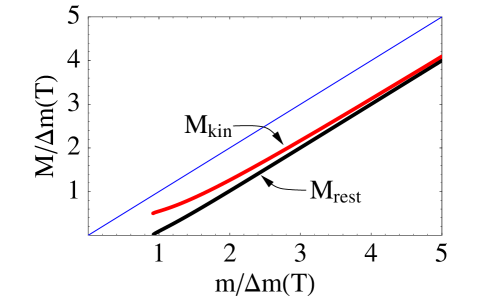
Figure 1: The thermal rest mass (or energy) $M_{\rm rest}$ and the kinetic mass $M_{\rm kin}$ of a quark immersed in the $\mathcal{N}\,{=}\,4$ plasma at temperature $T$, as functions of the zero-temperature mass $m$, with all masses measured in units of $\Delta m(T)={\textstyle\frac{1}{2}}\sqrt{\lambda}T$. At $m\approx 0.92\,\Delta m(T)$, the location of the D7-brane jumps discontinuously to the horizon [41, 42, 43, 44].

The dispersion relation of a moving quark in the thermal medium need not be Lorentz invariant since the plasma defines a preferred rest frame. For non-relativistic motion, the dispersion relation will have the form

$$E(p)=M_{\rm rest}(T)+\frac{p^{2}}{2M_{\rm kin}(T)}+\mathcal{O}(p^{4})\,.$$ (7)

The effective kinetic mass $M_{\rm kin}(T)$ is not the same as the thermal rest mass $M_{\rm rest}(T)$. For heavy quarks, we find that $M_{\rm kin}(T)$ differs negligibly from the thermal rest mass,

$$M_{\rm kin}(T)=M_{\rm rest}(T)+{\mathcal{O}}\Big{[}m\Big{(}\frac{\Delta m(T)}{m}\Big{)}^{\!2}\,\Big{]}\,,$$ (8)

but the difference between these masses becomes significant as the quark mass decreases. The dependence of the kinetic mass $M_{\rm kin}(T)$ on the quark mass is also shown in Figure 1. As $m/\Delta m(T)$ approaches the lower critical value of 0.92, the kinetic mass $M_{\rm kin}(T)$ has a limiting value just slightly greater than ${\textstyle\frac{1}{2}}\Delta m(T)$. As $m/\Delta m(T)\to\infty$, both $M_{\rm kin}$ and $M_{\rm rest}$ approach $m-\Delta m(T)$.

For not-so-heavy quarks moving relativistically, we can only infer the dispersion relation from analysis of the time-dependent numerical solutions discussed in Section 4. We do not have any analytic derivation, but all our numerical results are consistent with the thermal dispersion relation

$$E(p)=M_{\rm rest}(T)-M_{\rm kin}(T)+\sqrt{p^{2}+M_{\rm kin}(T)^{2}}\,,$$ (9)

which reduces to Eq. (7) for low momentum, and gives $v\equiv dE/dp=p/\sqrt{p^{2}+M_{\rm kin}(T)^{2}}$. For this relation between velocity and momentum, the viscous drag (2) is equivalent to $\dot{p}=-\mu p$ with a friction coefficient

$$\mu=\pi T\>\frac{\Delta m(T)}{M_{\rm kin}(T)}=\frac{\pi}{2}\,\frac{\sqrt{\lambda}\,T^{2}}{M_{\rm kin}(T)}\,.$$ (10)

As the quark mass decreases, the kinetic mass $M_{\rm kin}(T)$ has a lower limit of ${\textstyle\frac{1}{2}}\Delta m(T)$, and hence the friction coefficient has a remarkably simple upper limit,

$$\mu\leq 2\pi T\,,$$ (11)

which turns out to be dimension independent. It is tempting to speculate, along the lines of Ref. [34], that the ratio $\mu/T$ is bounded above by $2\pi$ even in more general theories.

Knowledge of the viscous drag on a quark is equivalent to knowledge of the diffusion constant for quark “flavor”. The relation is $D=T/(\mu M_{\rm kin})$, so our result (10) is equivalent to a flavor diffusion constant

$$D=\frac{1}{\pi\Delta m(T)}=\frac{2}{\pi\sqrt{\lambda}\,T}\,.$$ (12)

As discussed in Section 5, this same information may also be recast as the rate of change of the mean square transverse momentum of a quark initially moving in a given direction,

$$\frac{d}{dt}\,\left\langle(\vec{p}_{\perp})^{2}\right\rangle=\frac{4\,T^{2}}{D}=4\pi\Delta m(T)T^{2}=2\pi\sqrt{\lambda}\,T^{3}\,.$$ (13)

This quantity, divided by the velocity of the quark (to give a rate of change per unit distance traveled) is sometimes called the “jet quenching parameter” $\hat{q}$ [45].

Physically characterizing the mechanism responsible for the energy loss (10) in terms of some microscopic picture of the dynamics of the $\mathcal{N}\,{=}\,4$ SYM field theory is a challenge. In the AdS dual description, energy and momentum flow along the string which hangs down from the quark, away from the D7-brane and toward the black hole horizon. It is clear that the portion of the string which lies close to the horizon should be thought of as describing long distance deformations of the medium surrounding the quark. The energy loss should not be regarded as resulting from scattering off excitations in the thermal medium. Any scattering would correspond to small fluctuations in the string worldsheet, and these fluctuations are suppressed by inverse powers of the ’t Hooft coupling (or string tension). Nor is the energy loss due to radiation of glueballs, which correspond to closed strings breaking off of the open string and whose emission is suppressed by powers of $1/N_{\rm c}$. For relativistic velocities, $v\to 1$, there is nothing in the classical string dynamics which is reminiscent of near-collinear gluon bremsstrahlung which (at weak coupling) can cause a fast moving quark to lose an $\mathcal{O}(1)$ fraction of its momentum in a single scattering. Rather, the energy transfer from the moving quark to the surrounding plasma should be regarded as analogous to the formation of a wake in the coherent polarization cloud surrounding a charged particle moving through a polarizable medium, or the wake on the surface of water behind a moving boat.

Ultimately, the energy transfered to the medium from the moving quark must appear as heating and outward hydrodynamic flow in the non-Abelian plasma surrounding the quark. To see this flow directly, one would like to evaluate the expectation value of $T^{\mu\nu}(x)$ in the presence of the moving quark. The AdS/CFT correspondence provides a recipe for this calculation, but its implementation is difficult. The expectation value of $T^{\mu\nu}$ corresponds to boundary fluctuations in the gravitational metric. Deriving these fluctuations from the energy distribution of the string requires graviton propagators in the black hole geometry, for which no closed form analytic expression is currently available. Performing the computations required to evaluate $\langle T^{\mu\nu}(x)\rangle$ would allow one to examine the form of the wake behind a moving quark and, for example, see the sonic boom produced by a quark moving faster than the speed of sound. Sadly, we leave such a study for future work.

2 Open string dynamics in the black brane background

The AdS/CFT correspondence [30, 31, 32] posits an equivalence between $\mathcal{N}\,{=}\,4$ $SU(N_{\rm c})$ supersymmetric Yang-Mills theory and type IIB string theory in a $AdS_{5}\times S^{5}$ background. Type IIB strings are characterized by two numbers: a string coupling $g_{s}$ and a tension $T_{0}$, or equivalently a fundamental string length scale $\ell_{s}\equiv(2\pi T_{0})^{-1/2}$. The background is characterized by the radius of curvature of the $AdS_{5}$ and of the $S^{5}$, which must be equal and will be denoted by $L$.

The AdS/CFT correspondence provides a dictionary between these two seemingly very different physical theories. One important entry in this dictionary is the relationship between the string coupling and the Yang-Mills coupling,

$$4\pi g_{s}=g_{YM}^{2}\ ,$$ (14)

and an equally important entry is the relationship between the string tension, the radius of curvature $L$, and the ’t Hooft coupling,

$$\left({L}/{\ell_{s}}\right)^{4}=\lambda\equiv g_{YM}^{2}\,N_{\rm c}\ .$$ (15)

For the convenience of readers who are not completely conversant with the AdS/CFT correspondence, these relations, plus additional ones which will appear as we progress, are summarized in Table 1.

AdS	$\mathcal{N}{=}4$ SYM	quantity
$L$	–	$AdS_{5}$ and $S^{5}$ curvature radius
$\ell_{s}$	$\lambda^{-1/4}L$	fundamental string scale [${}\equiv\sqrt{\alpha^{\prime}}$]
$(L/\ell_{s})^{4}$	$\lambda$	’t Hooft coupling [${}\equiv g_{\rm YM}^{2}\,N_{\rm c}$]
$T_{0}$	$\frac{\sqrt{\lambda}}{2\pi}\,L^{-2}$	string tension [${}\equiv(2\pi\ell_{s}^{2})^{-1}$]
$g_{s}$	$\frac{1}{4\pi}\,g_{\rm YM}^{2}$	string coupling
$u_{h}$	$\pi T$	black hole horizon radius (${}\times L^{-2}$)
$u_{h}/\pi$	$T$	temperature
$u_{m}$	$\frac{2\pi}{\sqrt{\lambda}}\,(M_{\rm rest}{+}\Delta m)$	minimal radius of D7-brane (${}\times L^{-2}$)
$T_{0}L^{2}\,u_{h}$	$\Delta m(T)$	thermal rest mass shift [${}={\textstyle\frac{1}{2}}\sqrt{\lambda}T$]
$T_{0}L^{2}\,(u_{m}{-}u_{h})$	$M_{\rm rest}(T)$	static thermal quark mass

Table 1: AdS/CFT translation table. The static thermal quark mass $M_{\rm rest}(T)$ is the free energy of quark at rest in the $\mathcal{N}\,{=}\,4$ SYM plasma. It equals the Lagrangian quark mass $m$ in the zero temperature limit.

2.1 Adding a black hole

The gravity dual of finite temperature ${\mathcal{N}\,{=}\,4}$ $SU(N_{\rm c})$ super Yang-Mills theory is $S^{5}$ times the five dimensional AdS-black hole solution [33]. This solution is a geometry in which a black hole (or more properly, a black brane with a flat four dimensional horizon) is placed inside AdS space. The metric of the resulting AdS black brane solution in $d+1$ dimensions may be written as

$$ds^{2}=L^{2}\left(\frac{du^{2}}{h(u)}-h(u)\,dt^{2}+u^{2}\delta_{ij}\,dx^{i}dx^{j}\right),$$ (16)

where

$$h(u)=u^{2}\left[1-\left(\frac{u_{h}}{u}\right)^{d}\right].$$ (17)

Since the case of arbitrary dimension is usually as easy to compute as the specific $d=4$ case of interest, we will leave $d$ arbitrary in much of this section. Our radial coordinate $u$ has been rescaled by a factor of $L^{-2}$; some authors use $r=L^{2}\,u$ instead [46]. The black hole horizon is located at $u=u_{h}$ where $h(u)$ vanishes.

The Hawking temperature of the black hole equals the temperature of the field theory dual. The horizon radius is related to the Hawking temperature by

$$T=\frac{d}{4\pi}\,u_{h}\ ,$$ (18)

or $u_{h}=\pi\,T$ in $d=4$.

Introducing a flavor of fundamental representation quarks corresponds, in the gravity dual of the four dimensional field theory, to the addition of a D7-brane [38]. This D7-brane wraps an $S^{3}$ inside the transverse $S^{5}$ and fills all of the asymptotically $AdS$ space down to some minimum radial value $u=u_{m}$. We require that $u_{m}>u_{h}$. Given an open string that ends on this D7-brane, the quark is reinterpreted as the string’s endpoint. The choice of $u_{m}$ is equivalent to the choice of mass for the quark; the relation between $u_{m}$ and quark mass will be discussed in Section 3.

2.2 String equations of motion

The dynamics of an open string ending on the D7-brane depends on the background geometry, but the back reaction of the string on the geometry is negligible and may be neglected. The negligible back reaction reflects the fact that fundamental representation quarks only make an $\mathcal{O}(N_{\rm c})$ contribution to the free energy which is small, in the $N_{\rm c}\to\infty$ limit, relative to the $\mathcal{O}(N_{\rm c}^{2})$ contributions of the adjoint representation fields of $\mathcal{N}\,{=}\,4$ SYM.

The dynamics of a classical string is governed by the Nambu-Goto action,

$$S=-T_{0}\int d\sigma\>d\tau\sqrt{-\operatorname{det}{g_{ab}}}\ .$$ (19)

The coordinates $(\sigma,\tau)$ parametrize the induced metric $g_{ab}$ on the string world-sheet. Let $X^{\mu}(\sigma,\tau)$ be a map from the string world-sheet into space-time, and define $\dot{X}=\partial_{\tau}X$, $X^{\prime}=\partial_{\sigma}X$, and $V\cdot W=V^{\mu}W^{\nu}G_{\mu\nu}$ where $G_{\mu\nu}$ is the space-time metric (16). Then, writing $\operatorname{det}{g_{ab}}=g$, one has

$$-g=(\dot{X}\cdot X^{\prime})^{2}-(X^{\prime})^{2}(\dot{X})^{2}\ .$$ (20)

We will limit our attention to strings which lie within a three dimensional slice of the asymptotically AdS space in which all but one (call it $x$) of the transverse coordinates $x^{i}$ vanish. So $X(\sigma,\tau)$ will be a map to $(t,u,x)$. Choosing a static gauge where $\sigma=u$ and $\tau=t$, the string worldsheet is described by a single function $x(u,t)$. With this choice, one finds that

$$\dot{X}\cdot X^{\prime} = L^{2}\left(u^{2}\dot{x}x^{\prime}\right),$$ (21a)

$$(X^{\prime})^{2} = L^{2}\left[h^{-1}+u^{2}(x^{\prime})^{2}\right],$$ (21b)

$$(\dot{X})^{2} = L^{2}\left[-h+u^{2}(\dot{x})^{2}\right],$$ (21c)

and the induced metric becomes

$$g_{ab}=L^{2}\left[\begin{array}[]{cc}-h+u^{2}(\dot{x})^{2}&u^{2}\,\dot{x}x^{\prime}\\ u^{2}\,\dot{x}x^{\prime}&\frac{1}{h}+u^{2}(x^{\prime})^{2}\end{array}\right]\ .$$ (22)

The determinant of $g_{ab}$ is

$$-\frac{g}{L^{4}}=1-h^{-1}\,{u^{2}}(\dot{x})^{2}+h\,u^{2}(x^{\prime})^{2}\ .$$ (23)

From this determinant, the equation of motion that follows from the Nambu-Goto action is

$$\frac{\partial}{\partial u}\left(h\,u^{2}\frac{x^{\prime}}{\sqrt{-g}}\right)-\frac{u^{2}}{h}\frac{\partial}{\partial t}\left(\frac{\dot{x}}{\sqrt{-g}}\right)=0\ .$$ (24)

Useful to us in the following are general expressions for the canonical momentum densities associated to the string,

$$\pi^{0}_{\mu} = -T_{0}\,G_{\mu\nu}\,\frac{(\dot{X}\cdot X^{\prime})(X^{\nu})^{\prime}-(X^{\prime})^{2}(\dot{X}^{\nu})}{\sqrt{-g}}\ ,$$ (25a)

$$\pi^{1}_{\mu} = -T_{0}\,G_{\mu\nu}\,\frac{(\dot{X}\cdot X^{\prime})(\dot{X}^{\nu})-(\dot{X})^{2}(X^{\nu})^{\prime}}{\sqrt{-g}}\ .$$ (25b)

For our string, these expressions reduce to

$$\left(\begin{array}[]{c}\pi^{0}_{x}\\ \pi^{0}_{u}\\ \pi^{0}_{t}\end{array}\right)=\frac{T_{0}L^{4}}{\sqrt{-g}}\left[\begin{array}[]{c}\dot{x}\,u^{2}\,h^{-1}\\ -\dot{x}\,x^{\prime}\,u^{2}\,h^{-1}\\ -1-(x^{\prime})^{2}\,u^{2}\,h\end{array}\right],\quad\left(\begin{array}[]{c}\pi^{1}_{x}\\ \pi^{1}_{u}\\ \pi^{1}_{t}\end{array}\right)=\frac{T_{0}L^{4}}{\sqrt{-g}}\left[\begin{array}[]{c}-x^{\prime}\,u^{2}\,h\\ -1+(\dot{x})^{2}u^{2}\,h^{-1}\\ \dot{x}\,x^{\prime}\,u^{2}\,h\end{array}\right].$$ (26)

The density of energy and $x$-component of momentum on the string worldsheet are given by $\pi^{0}_{t}$ and $\pi^{0}_{x}$, respectively. Integrating them along the string gives the total energy and momentum of the string,

$$E=-\int d\sigma\>\pi_{t}^{0}\,,\qquad p=\int d\sigma\>\pi_{x}^{0}\ .$$ (27)

3 Single quark solutions

3.1 Static strings

Single quark solutions correspond to strings which hang from the D7-brane down to the black hole horizon. The simplest solution to the string equation of motion (24) is just a constant, $x(u,t)=x_{0}$. This solution describes a static string stretching from $u=u_{m}$ straight down to the black hole horizon at $u_{h}$, and clearly represents a static quark at rest in the thermal medium. We may compute the energy and momentum of such a configuration using Eq. (27). The energy

$$E=T_{0}L^{2}\int_{u_{h}}^{u_{m}}du=T_{0}L^{2}\,(u_{m}-u_{h})\,,$$ (28)

while the total momentum $p$ (and momentum density $\pi^{0}_{x}$) vanish. This energy must equal the (Lagrangian) mass $m$ of the quark in the zero temperature limit. Recalling, from Eq. (18), that $u_{h}$ is proportional to the temperature, we see that

$$T_{0}L^{2}\,u_{m}=m\qquad\mbox{(zero temperature)}\,.$$ (29)

Moving the D7-brane to a larger radius (larger $u_{m}$) increases the mass of the quark; a D7-brane sitting at the boundary of the (asymptotically) AdS space corresponds to quarks of infinite mass.

However, raising the temperature affects the relation between the Lagrangian mass $m$ and the position $u_{m}$ of the D7-brane in the gravitational description. The result has the form

$$\frac{T_{0}L^{2}\,u_{m}}{m}=1+g\Big{(}\frac{T_{0}L^{2}u_{h}}{m}\Big{)}\,,$$ (30)

with the correction $g(x)$ behaving (for $d=4$) as

$$g(x)=\frac{1}{8}\,x^{4}-\frac{5}{128}\,x^{8}+\mathcal{O}(x^{12})\,.$$ (31)

Retaining just the first two terms in $g(x)$ gives a result for $T_{0}L^{2}u_{m}/m$ which is accurate to within 1%.

The energy (28) of the static string should be interpreted as the free energy of a static quark sitting in the thermal $\mathcal{N}\,{=}\,4$ SYM medium. In a small abuse of language, we will refer to this free energy as the static thermal mass, $M_{\rm rest}(T)$. Using $u_{h}=\pi T$ [from Eq. (18)] plus $T_{0}L^{2}=\frac{\sqrt{\lambda}}{2\pi}$, the result is

$$M_{\rm rest}(T) \equiv T_{0}L^{2}\,(u_{m}-u_{h})$$ (32a)

$$= m-\Delta m(T)+m\,g\Big{(}\frac{\Delta m(T)}{m}\Big{)}\,,$$

with

$$\Delta m(T) \equiv T_{0}L^{2}u_{h}={\textstyle\frac{1}{2}}\sqrt{\lambda}T\,.$$ (32b)

This relation between the static thermal mass $M_{\rm rest}(T)$ and the Lagrangian mass $m$ is plotted in Figure 1.

3.2 Moving, straight strings

A rigidly moving string profile $x(u,t)=x_{0}+vt$ is also a solution to the string equation of motion (24). However, such rigid motion of the string is not physical. The problem is that $-g$ is not positive definite for this profile. One finds that $g$ vanishes at a critical value $u_{c}$ given by

$$(u_{c})^{d}=\frac{(u_{h})^{d}}{1-v^{2}}\,.$$ (33)

For any non-zero velocity, $u_{c}>u_{h}$ and $-g$ is negative in the region $u_{h}<u<u_{c}$ between the horizon and the critical value of the radius. A negative determinant is often a signal of superluminal propagation. When $g=0$ the induced metric on the string world sheet is degenerate, and if $-g<0$ then the action, energy, and momentum all become complex, which means this solution must be discarded. By choosing $x=vt$, we picked inconsistent initial conditions where parts of the string have a velocity faster than the local speed of light at $t=0$. While time evolution of this initial configuration gives a very simple solution, it is not physical.

3.3 Moving, curved strings

To find a physical configuration which corresponds to a quark moving at constant velocity, we will look for stationary solutions of the form

$$x(u,t)=x(u)+vt\,.$$ (34)

For string profiles of this form, $x^{\prime}$, $\dot{x}$, and $\sqrt{-g}$ are time-independent. The time derivative term in the equation of motion (24) completely drops out and we are left with an ordinary differential equation

$$\frac{d}{du}\left(h\,u^{2}\frac{x^{\prime}}{\sqrt{-g}}\right)=0$$ (35)

where

$$\sqrt{-g}=L^{2}\left[1-h^{-1}\,u^{2}\,v^{2}+h\,u^{2}\,(x^{\prime})^{2}\right]^{1/2}\,.$$ (36)

This differential equation is straightforward to integrate. (The $v=0$ limit of this equation appeared in the finite temperature calculation [47, 48] of the AdS Wilson line [49, 50].) The first integral is

$$\frac{x^{\prime}}{\sqrt{-g/L^{4}}}\,=\frac{C\,v}{u^{2}\,h}\,,$$ (37)

or

$$(x^{\prime})^{2}=\frac{C^{2}\,v^{2}}{u^{8}}\left[1-(u_{h}/u)^{d}\right]^{-2}\>\frac{1-v^{2}-(u_{h}/u)^{d}}{1-C^{2}\,v^{2}\,u^{-4}-(u_{h}/u)^{d}}\,,$$ (38)

where $C$ is an integration constant. This constant determines the momentum current flowing along the string. From the expressions (26) for these currents, we see that

$$\pi_{x}^{1}=-T_{0}L^{2}\,C\,v\,,\qquad\pi_{t}^{1}=T_{0}L^{2}\,C\,v^{2}\,,$$ (39)

showing that these two currents are constant along the length of the string.

Solving for $-g$ yields

$$\frac{-g}{L^{4}}=\frac{1-v^{2}-(u_{h}/u)^{d}}{1-C^{2}\,v^{2}\,u^{-4}-(u_{h}/u)^{d}}\ .$$ (40)

Both numerator and denominator are positive for large $u$, and negative for $u$ near $u_{h}$. So the only way for $-g$ to remain positive everywhere on a string that stretches from the boundary to the horizon is to have both numerator and denominator change sign at the same point. This condition uniquely fixes $C$ up to a sign,

$$C=\pm\left(\frac{u_{h}^{d}}{1-v^{2}}\right)^{2/d}\quad\mathop{\longrightarrow}\limits^{d=4}\quad\pm\frac{u_{h}^{2}}{\sqrt{1-v^{2}}}\ .$$ (41)

For the specific case of $d=4$, $-g/L^{4}$ reduces to $1-v^{2}$, and we have

$$x^{\prime}(u)=\pm v\,\frac{u_{h}^{2}}{h(u)\,u^{2}}\ .$$ (42)

Integrating $x^{\prime}$ yields solutions of the form

$$x(u,t)=x_{\pm}(u,t)\equiv x_{0}\pm v\,F(u;v^{2})+vt\,,$$ (43)

where the upper sign corresponds to $C$ positive; the lower to $C$ negative, and $x_{0}$ is the position of the string at the $u=\infty$ boundary at time zero. For arbitrary $d$, $F(u;v^{2})$ is a hypergeometric function. For $d=4$, this function reduces to the velocity independent expression,

$$F(u)=\frac{1}{2\,u_{h}}\left[\frac{\pi}{2}-\mbox{arctan}\!\left(\frac{u}{u_{h}}\right)-\mbox{arccoth}\!\left(\frac{u}{u_{h}}\right)\right].$$ (44)

This function is plotted in Figure 2. It vanishes as $u\to\infty$ and diverges to $-\infty$ as $u\to u_{h}$; its asymptotic behavior is

$$F(u)=\begin{cases}\displaystyle-\frac{u_{h}^{2}}{3u^{3}}+O\Big{(}\frac{u_{h}^{6}}{u^{7}}\Big{)}\,,&u\to\infty\,;\\[10.0pt] \displaystyle-\frac{1}{4u_{h}}\ln\Big{(}\frac{2u_{h}}{u{-}u_{h}}\Big{)}+\frac{\pi}{8u_{h}}+O\Big{(}\frac{u{-}u_{h}}{u_{h}^{2}}\Big{)}\,,&u\to u_{h}\,.\end{cases}$$ (45)

Figure 2: A plot of the function $F(u)$ which determines the string profile, in units where $u_{h}=1$.

Figure 3: Schematic drawing of the physical solution (left) in which energy flows toward the horizon, and the unphysical energy solution (right) in which energy flows away from the horizon.

The rate at which energy flows down the string is given by $\pi^{1}_{t}$. As seen in Eq. (39), this energy flux is proportional to $C$. If $C$ is positive, then energy flows down the string toward the horizon, and the string profile resembles a tail being dragged behind the moving quark, as illustrated on the left in Figure 3. If $C$ is negative, then one has the time-reversed situation: energy flows upward from the horizon and the tail of string leads the quark. We postulate (as in Ref. [51]) that the physical process we want to describe requires us to pick purely outgoing boundary conditions at the horizon. We have to discard the time-reversed solution in which energy flows from the black hole to the moving quark.

The resulting rates at which energy and momentum flow toward the horizon are

$$\left.\pi^{1}_{t}\right|_{u=u_{h}} = T_{0}L^{2}\,u_{h}^{2}\,\frac{v^{2}}{(1-v^{2})^{2/d}}\quad\mathop{\longrightarrow}\limits^{d=4}\quad{\textstyle\frac{\pi}{2}}\sqrt{\lambda}\,T^{2}\,\frac{v^{2}}{\sqrt{1-v^{2}}}\,,$$ (46a)

and

$$\left.-\pi^{1}_{x}\right|_{u=u_{h}} = T_{0}L^{2}\,u_{h}^{2}\,\frac{v}{(1-v^{2})^{2/d}}\quad\mathop{\longrightarrow}\limits^{d=4}\quad{\textstyle\frac{\pi}{2}}\sqrt{\lambda}\,T^{2}\,\frac{v}{\sqrt{1-v^{2}}}\,,$$ (46b)

respectively.

The stationary solution $x_{+}(u,t)$ given by Eqs. (43) and (44) describes an open string which runs from the AdS boundary at $u=\infty$ and asymptotically approaches the horizon at $u=u_{h}$. By truncating the solution at an arbitrary radius $u_{m}>u_{h}$, one may equally well regard it as describing an open string running from a D7-brane with minimal radius $u_{m}$ down to the horizon. The rates (46) at which energy and momentum flow down the string are completely independent of $u_{m}$.

Standard Neumann boundary conditions would demand that the momentum flux $\pi_{x}^{1}$ vanish at the flavor brane — so our solution with a constant non-zero $\pi_{x}^{1}$ does not satisfy Neumann boundary conditions. The solution is physical, but there must be a force acting on the string endpoint and feeding energy and momentum into the string. A constant electric field on the flavor brane provides precisely such a force. The field alters the Neumann boundary condition to the force balance condition $\pi_{x}^{1}=-F_{tx}$.

Although the flux of energy and momentum in this stationary solution is finite, the total energy and momentum of the string is infinite, due to the contribution to the integrals (27) close to the horizon. If one simply inserts a lower limit $u_{\rm min}>u_{h}$, together with an upper limit equal to the radius $u_{m}$ of the D7-brane, then the resulting energy and momentum (in $d=4$) are

$$E = -\int_{u_{\rm min}}^{u_{m}}du\>\pi^{0}_{t}(u)=T_{0}L^{2}\,\frac{1}{\sqrt{1-v^{2}}}\,\left[u_{m}-u_{\rm min}+v^{2}\Lambda(u_{\rm min})\right],$$ (47a)

$$p = \int_{u_{\rm min}}^{u_{m}}du\>\pi^{0}_{x}(u)=T_{0}L^{2}\,\frac{v}{\sqrt{1-v^{2}}}\,\left[u_{m}-u_{\rm min}+\Lambda(u_{\rm min})\right]\ ,$$ (47b)

where

$$\Lambda(u_{\rm min})\equiv\frac{u_{h}}{4}\!\left[\,2\,\mbox{arctan}\,\frac{u_{min}}{u_{h}}-2\,\mbox{arctan}\,\frac{u_{m}}{u_{h}}-\ln\frac{(u_{m}+u_{h})(u_{min}-u_{h})}{(u_{m}-u_{h})(u_{min}+u_{h})}\right].$$ (48)

As $u_{\rm min}\to u_{h}$, this function diverges logarithmically as $-{\textstyle\frac{1}{4}}\,u_{h}\ln(u_{\rm min}{-}u_{h})$. The interpretation of this IR divergence will be discussed momentarily.

Field theory interpretation

We want to interpret this stationary string solution as describing the steady-state behavior of a massive quark moving through the $\mathcal{N}\,{=}\,4$ plasma under the influence of a constant electric field ${\cal E}=F_{tx}$. The quark velocity will asymptotically approach an equilibrium value $v$ at which the rate of momentum loss to the plasma is balanced by the driving force exerted by the electric field. The rate at which the electric field does work on the quark, namely $v\cdot{\cal E}$, should also equal the rate at which the quark loses energy to the medium. The results (46), plus the force balance condition at the string endpoint,

$$\pi^{1}_{x}=-\cal E\,,$$ (49)

are completely consistent with this interpretation, provided one regards energy and momentum flow toward the horizon as energy and momentum transfer to the thermal medium.

If the quark behaves as an excitation with some effective mass $M$ and momentum $p=Mv/\sqrt{1-v^{2}}$, then the result (46b) for the momentum transfer rate is equivalent to a momentum loss rate ${dp}/{dt}=-\mu p$ for the quark, with

$$\mu M={\textstyle\frac{\pi}{2}}\sqrt{\lambda}T^{2}=\pi T\,\Delta m(T)\,.$$ (50)

Just as in the toy model discussed in the Introduction, the momentum flow of our steady state solution determines $\mu M$, but not $\mu$ or $M$ individually. Note that $\mu M$ is independent of the flavor brane location $u_{m}$, and hence is independent of the physical quark mass.

The energy of the string should be regarded as the total excess free energy of the system — the free energy minus its equilibrium value at the given temperature. In other words, the energy of string includes all the effects of the disturbance to the $\mathcal{N}\,{=}\,4$ plasma produced by the moving quark. The stationary moving string solution is describing a system in which a quark has been forcibly dragged through the plasma (which is infinite in extent) for an unbounded period of time. The constant rate of work done by the external electric field thus translates into an infinite input of energy to the plasma. This unbounded input of energy is the physical origin of the IR divergence in the string energy, as may be seen explicitly by noting that the logarithmically divergent function $\Lambda(u_{\rm min})$ appearing in the energy and momentum (47) is proportional to the difference in position (in $x$) between the two ends of the cut-off string,

$$\Lambda(u_{\rm min}) = u_{h}^{2}\,\left|\frac{\Delta x(u_{\rm min})}{v}\right|$$ (51)

with

$$\Delta x(u_{\rm min}) \equiv x_{+}(u_{m},t)-x_{+}(u_{\rm min},t)\,.$$ (52)

Comparison with Eq. (46) shows that the cut-off string energy and momentum are just a boosted static energy plus the net input of energy and momentum required to move the quark a distance $\Delta x$ at velocity $v$,

$$E = T_{0}L^{2}\>\frac{(u_{m}{-}u_{\rm min})}{\sqrt{1-v^{2}}}\,+\frac{1}{v}\,\frac{dE}{dt}\>\Delta x(u_{\rm min})\,,$$ (53a)

$$p = T_{0}L^{2}\>\frac{v\,(u_{m}{-}u_{\rm min})}{\sqrt{1-v^{2}}}+\frac{1}{v}\,\frac{dp}{dt}\>\Delta x(u_{\rm min})\,,$$ (53b)

where $dE/dt=\pi^{1}_{t}$ and $dp/dt=-\pi^{1}_{x}$ are the rates at which the external electric field transfers energy and momentum to the quark. Note that the $u_{\rm min}\to u_{h}$ limit of $T_{0}L^{2}(u_{m}{-}u_{\rm min})$ is just the static rest energy $M_{\rm rest}(T)$.

The result (53) suggests that one might interpret $M_{\rm rest}(T)/\sqrt{1-v^{2}}$ as the energy (and $v$ times this as the momentum) of a quark moving at velocity $v$ through the plasma. Or equivalently, that the appropriate thermal dispersion relation is just a relativistic dispersion relation but with mass $M_{\rm rest}(T)$. This, we believe, is too simplistic. A quark moving through the thermal plasma is a quasiparticle — an elementary excitation of the system with a finite thermal width given by the damping rate $\mu$. The (free) energy of a quark moving through the medium is only defined to within an uncertainty given by its thermal width. A natural operational definition is to start with a static quark, at rest in the thermal medium, turn on an electric field which accelerates the quark to the desired velocity in some time $\tau$, and then define the energy of the quark as its initial rest energy plus the work done by the electric field while accelerating the quark. The acceleration time $\tau$ should be small compared to the damping time $\mu^{-1}$, to avoid counting energy which has already been lost to the medium. But $\tau$ should also be large compared to the inverse kinetic energy of the quark, to minimize the quantum uncertainty in the energy. Satisfying both conditions is only possible if the thermal width is small compared to the energy, which is the basic condition defining a good quasiparticle. Choosing $\tau\sim(\mu Mv^{2})^{-1/2}$ (for non-relativistic motion) balances the two uncertainties and gives a limiting precision with which one can define the kinetic energy of a moving quark that scales as $\lambda^{1/4}\,T/p$. Finding the requisite string solution with such a time-dependent electric field has not (yet) been done.

3.4 Quasinormal modes

Instead of considering a quark moving under the influence of an external electric field, we now turn to the motion of a quark decelerating in the thermal medium, in the absence of any external forcing. The setup here is the analog of the second gedanken experiment for the toy model discussed in the Introduction. We will focus on the late-time, and hence low-velocity, behavior. We extract this late-time dynamics by analyzing small perturbations to the static string which describes a quark at rest. A key ingredient will be the purely outgoing boundary conditions at the horizon which capture the dissipative nature of the process and have been shown to reproduce appropriate thermal physics [51]. With these boundary conditions, the problem becomes a quasinormal mode calculation on the string worldsheet. To complement the linear analysis of this section, in Section 4 we will also perform a numerical analysis of the full, time-dependent problem.

The linearized equation of motion for small fluctuations around the static straight string, $x(u,t)=x_{0}$ means treating $\dot{x}$ and $x^{\prime}$ as small and retaining only terms linear in derivatives of $x$. From Eq. (23) one sees that this corresponds to replacing $-g/L^{4}$ with 1, which reduces the full string equation of motion (24) to

$$\frac{\partial}{\partial u}\left(hu^{2}x^{\prime}\right)=\frac{u^{2}}{h}\,\ddot{x}\,.$$ (54)

To select the physically relevant solution, we impose purely outgoing boundary conditions at the horizon. These boundary conditions make the resulting boundary value problem non-hermitian and the resulting quasinormal modes will have real exponential time dependence. Close to the horizon, the most general solution of the wave equation (54) has the form

$$x(u,t)=F\Big{(}t+\frac{1}{u_{h}d}\log(\epsilon)\Big{)}+G\Big{(}t-\frac{1}{u_{h}d}\log(\epsilon)\Big{)}\ .$$ (55)

where $\epsilon\equiv u/u_{h}-1$ [or $u=(1+\epsilon)u_{h}$], and $F(x)$ and $G(x)$ are arbitrary (differentiable) functions. Purely outgoing means that $G=0$ in this regime.

Specializing to $e^{-\mu t}$ time dependence and introducing, for convenience, a dimensionless radial coordinate $y\equiv u/u_{h}$ and dimensionless decay rate $\gamma=\mu/u_{h}$, the linearized wave equation (54) becomes the eigenvalue equation

$$\mathcal{L}\,x=\gamma^{2}\,x\,,$$ (56a)

with (56b)

$$\mathcal{L}\equiv(1-y^{-d})\,\frac{d}{dy}\,y^{4}(1-y^{-d})\,\frac{d}{dy}\,.$$

Imposing outgoing boundary conditions at the horizon and Neumann boundary conditions at the flavor brane leads to a discrete spectrum of quasinormal mode decay rates.

Close to the horizon at $y=1$, the purely outgoing solution to Eq. (56) is proportional to $(y{-}1)^{-\gamma/d}$ with $\gamma$ positive. This diverges as $y\to 1$, showing that there are non-uniformities between the large time and near horizon limits. In particular, the assumption that $\sqrt{-g}/L^{2}\approx 1$ is only valid at sufficiently late times, when $t+(u_{h}d)^{-1}\log(y{-}1)$ is sufficiently large. To evaluate the deviation of $\sqrt{-g}/L^{2}$ from unity, one needs the next-to-leading term in the near horizon asymptotics. We find $x(y,t)=A(y{-}1)^{-\gamma/d}e^{-\gamma u_{h}t}\left\{1+\gamma B(y{-}1)+\mathcal{O}[(y{-}1)^{2}]\right\}$ with $B=\frac{3-d}{2d}+\frac{2}{d-2\gamma}$. This gives

$$\frac{-g}{L^{4}}=1-\frac{4A^{2}\mu^{2}}{d{-}2\gamma}\,(y{-}1)^{-2\gamma/d}\,e^{-2\mu t}\times[1+{\mathcal{O}}(y{-}1)]\,,$$

which shows that, at any fixed position outside the horizon, $\sqrt{-g}/L^{2}\approx 1$ for sufficiently large times.

The near horizon asymptotics are useful also for exploring the small mass limit $y_{m}\to 1$ of our quasinormal mode problem. It is possible for $x(y,t)$ to obey Neumann boundary conditions at $y=y_{m}$, in the limit $y_{m}\to 1$, if $\gamma={\textstyle\frac{d}{2}}+\mathcal{O}(y_{m}{-}1)$. This enables the first two terms in the asymptotic series expansion for $x(y,t)$ to give comparable, and canceling, contributions to the slope $x^{\prime}(y_{m},t)$. This result, $\gamma\to{\textstyle\frac{d}{2}}$, gives the intercepts of the $d=4$ and $d=2$ curves shown below in Figure 4. Converting from the dimensionless decay rate $\gamma$ back to $\mu$ yields the result, valid for all $d$, that $\mu=2\pi T$ in the limit where the flavor brane approaches the horizon.

Large mass limit

The differential equation (56) does not appear to have a simple solution for arbitrary $d$. In the special case of $d=2$, the differential equation can be solved in terms of associated Legendre functions, as discussed in Appendix B. For the $d=4$ case of interest, Eq. (56) is a particular example of the Heun equation, a differential equation with four regular singular points. Heun functions are difficult to work with, and other values of $d$ appear to be even more difficult to treat analytically.

In the absence of a simple analytic solution to Eq. (56), we attempt a power series solution in $\gamma$,

$$x(y)=x_{0}(y)+\gamma\,x_{1}(y)+\gamma^{2}\,x_{2}(y)+\cdots\,.$$ (57)

We will focus on the large mass regime where the flavor brane position $y_{m}\equiv u_{m}/u_{h}\gg 1$, and we will find an iterative solution where $\gamma=\mathcal{O}(1/y_{m})$. For the moment, the correlation between $\gamma$ and $y_{m}$ may be viewed as an assumption which will be verified a posteriori. Requiring $\mathcal{L}\,x=\gamma^{2}\,x$ implies that

$${\mathcal{L}}\,x_{0}=0\,,\quad{\mathcal{L}}\,x_{1}=0\,,\quad\mbox{and}\quad{\mathcal{L}}\,x_{2}=x_{0}\,.$$ (58)

We want to satisfy Neumann boundary conditions at the flavor brane, $x^{\prime}(y_{m})=0$, together with outgoing boundary conditions at the horizon. As seen above, this requires that $x(y)\sim A\,(y{-}1)^{-\gamma/d}$ as $y\to 1$, for some constant $A$, or equivalently

$$x^{\prime}(y)\sim-A\,\frac{\gamma}{d}\,(y{-}1)^{-1-\gamma/d}=A\left[-\frac{\gamma}{d}\,\frac{1}{y{-}1}+\frac{\gamma^{2}}{d^{2}}\,\frac{\ln(y{-}1)}{y{-}1}+\mathcal{O}(\gamma^{3})\right].$$ (59)

The constant $x_{0}(y)=A$ is the only homogeneous solution which obeys Neumann boundary conditions at the flavor brane at $y=y_{m}$. To generate the $\mathcal{O}(\gamma)$ term in the near horizon behavior (59), the first order correction $x_{1}(y)$ must equal the second homogeneous solution of $\mathcal{L}\,x=0$. The derivative of this homogeneous solution (which will be sufficient for our purposes) is

$$x_{1}^{\prime}(y)=-A\,\frac{y^{d-4}}{y^{d}{-}1}\,.$$ (60)

At the flavor brane, $x_{1}^{\prime}(y_{m})=-A\,y_{m}^{-4}+\mathcal{O}(y_{m}^{-4-d})$. This violates the Neumann boundary conditions. However, if $\gamma=\mathcal{O}(1/y_{m})$, then this violation can, and will, be compensated by the next order term. Moving on to $x_{2}(y)$ and solving $\mathcal{L}\,x_{2}=x_{0}$ gives

$$x_{2}^{\prime}(y)=A\,\frac{y^{d-3}}{y^{d}{-}1}\left[1-{}_{2}F_{1}\left({\textstyle\frac{1}{d}},1,{\textstyle\frac{d+1}{d}};y^{d}\right)\right]+C\,\frac{y^{d-4}}{y^{d}{-}1}\,.$$ (61)

As $y\to 1$, the leading term in the hypergeometric function is

$${}_{2}F_{1}\left({\textstyle\frac{1}{d}},1,{\textstyle\frac{d+1}{d}};y^{d}\right)=-\frac{1}{d}\,\ln(y{-}1)+{\mathcal{O}}(1)\ ,$$ (62)

and so

$$x_{2}^{\prime}(y)=\frac{A}{d^{2}}\frac{1}{y{-}1}\Big{[}\ln(y{-}1)+\mathcal{O}(1)\Big{]}.$$ (63)

The logarithmic term is precisely what is required to generate the $\mathcal{O}(\gamma^{2})$ term in the outgoing boundary condition (59). The unwanted non-logarithmic $(y{-}1)^{-1}$ term is eliminated by an appropriate choice for the coefficient $C$ of the homogeneous term in (61).

When evaluated at $y_{m}\gg 1$, the hypergeometric function is negligible compared to 1,

$${}_{2}F_{1}\left({\textstyle\frac{1}{d}},1,{\textstyle\frac{d+1}{d}};y_{m}^{d}\right)={\mathcal{O}}(1/y_{m})\,,$$ (64)

so that

$$x_{2}^{\prime}(y_{m})=A\,y_{m}^{-3}+\mathcal{O}(y_{m}^{-4})\,.$$ (65)

The Neumann boundary condition requires

$$0=x^{\prime}(y_{m})=\gamma\,x_{1}^{\prime}(y_{m})+\gamma^{2}\,x_{2}^{\prime}(y_{m})+\cdots\,.$$ (66)

Inserting the explicit forms (60) and (65), one sees that the leading $\gamma/y_{m}^{4}$ term from $x_{1}^{\prime}(y_{m})$ will cancel the leading $\gamma^{2}/y_{m}^{3}$ term from $x_{2}^{\prime}(y_{m})$ provided

$$\gamma=\frac{1}{y_{m}}+{\mathcal{O}}\left(1/{y_{m}^{2}}\right).$$ (67)

This value of $\gamma^{2}$ is the smallest eigenvalue of $\cal L$ (for the given boundary conditions). All other eigenvalues are $\mathcal{O}(1)$ as $y_{m}\to\infty$. Expressing the result (67) in terms of the original variables, the lowest quasinormal mode decay rate is

$$\mu=\frac{u_{h}^{2}}{u_{m}}+\mathcal{O}(u_{h}^{3}/u_{m}^{2})\,.$$ (68)

The motion of the string endpoint in this quasinormal mode is a simple exponential,

$$x(u_{m},t)-x_{0}\propto A\,e^{-\mu t}\,,$$ (69)

so the velocity of the string endpoint satisfies

$$\dot{v}=-\mu\,v\,.$$ (70)

Inserting the result (68) for $\mu$ and using the large mass limit of the relation (30) between the brane position and quark mass, namely $u_{m}=m/(T_{0}L^{2})$, converts this result to

$$\frac{dp}{dt}=-(T_{0}L^{2}\,u_{h}^{2})\,v\,,$$ (71)

with $p=mv$. This agrees perfectly with our earlier result (46b) at small $v$.

Arbitrary mass

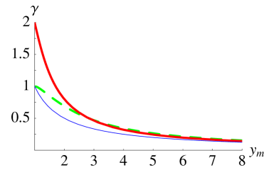
Figure 4: Lowest quasinormal mode decay rate $\gamma$ as a function of mass parameter $y_{m}$, for $d=2$ (green dashed line) and $d=4$ (thick red solid line), together with the leading large mass analytic form $\gamma=\frac{1}{y_{m}}$ (thin blue line)

To find the lowest eigenvalue of the quasinormal mode operator $\mathcal{L}$ for an arbitrary D7-brane location $y_{m}$, it is necessary to resort to numerical analysis. A simple shooting algorithm suffices. At a point close to the horizon, $y=1+\epsilon$ with $\epsilon\ll 1$, one sets $x(1{+}\epsilon)=1$ and $x^{\prime}(1{+}\epsilon)=-\frac{\gamma}{d}\frac{1}{\epsilon}$. This enforces the outgoing boundary condition. Then, for various values of $\gamma$, one integrates the differential equation $(\mathcal{L}-\gamma^{2})\,x=0$ out to the flavor brane, and successively refines $\gamma$ to locate the minimal value that satisfies the Neumann boundary condition $x^{\prime}(y_{m})=0$.

In Figure 4 we plot the resulting lowest quasinormal decay rate, as a function of the flavor brane location $y_{m}$, in dimensions $d=2$ and 4. These numerical values are consistent with our large mass result that $\gamma=y_{m}^{-1}+\mathcal{O}(y_{m}^{-2})$. In Appendix B, we show that the $d=2$ case is analytically soluble, and the resulting frequencies satisfy the equation

$$y_{m}=\frac{1}{\gamma}-\frac{\gamma}{2}+{\mathcal{O}}(\gamma^{2})\ .$$ (72)

When we compare the actual shape $x(u,t)$ of the QNM with the analytic stationary solution, we find that they agree when $\gamma\ll 1$ (that is for large mass), which is when the external field needed to maintain the velocity is small.

Low velocity dispersion relation

In addition to extracting the lowest quasinormal mode decay rate, the linearized equation of motion (54) may also be used to find the dispersion relation of a quark moving at low velocity. If $\dot{x}$ and $x^{\prime}$ are small, so that $\sqrt{-g/L^{4}}\approx 1$, then the momentum density $\pi_{x}^{0}=T_{0}L^{2}\,u^{2}\,h^{-1}\,\dot{x}$. For a quasinormal mode with exponential time dependence, $x(u,t)=x(u)\,e^{-\mu t}$, the momentum density may be rewritten as

$$\pi_{x}^{0}=-\frac{T_{0}L^{2}}{\mu}\>u^{2}\,h^{-1}\>\ddot{x}=-\frac{T_{0}L^{2}}{\mu}\>(hu^{2}x^{\prime})^{\prime}\,,$$ (73)

where the last form follows from the linearized equation of motion (54). This current is easily integrated to find the total momentum carried by the portion of the string running from the flavor brane down to an IR cutoff $u_{\rm min}>u_{h}$,

$$p=\int_{u_{\rm min}}^{u_{m}}du\>\pi_{x}^{0}=\frac{T_{0}L^{2}}{\mu}\>hu^{2}x^{\prime}\Big{|}^{u=u_{m}}_{u=u_{\rm min}}\ .$$ (74)

Because of the Neumann boundary conditions, the upper endpoint does not contribute. Hence

$$p=\frac{T_{0}L^{2}}{\mu}\>h(u_{\rm min})\,u_{\rm min}^{2}\,x^{\prime}(u_{\rm min})\,.$$ (75)

The energy may be evaluated similarly. We are interested in the deviation of the energy from the static rest energy, and it is therefore necessary to keep all terms up to quadratic order in $\dot{x}$ and $x^{\prime}$ in the energy density $\pi_{t}^{0}$. Suitably expanding $\sqrt{-g/L^{4}}$, the energy density is

$$\pi_{t}^{0}=-T_{0}L^{2}\Big{[}1+{\textstyle\frac{1}{2}}hu^{2}(x^{\prime})^{2}+{\textstyle\frac{1}{2}}\mu^{2}\,h^{-1}u^{2}x^{2}+\mathcal{O}(x^{4})\Big{]}\,.$$ (76)

Using the linearized equation of motion (54), one may express the resulting energy solely as endpoint contributions,

$$E=-\int_{u_{\rm min}}^{u_{m}}du\>\pi_{t}^{0}=T_{0}L^{2}\Big{[}(u_{m}-u_{\rm min})-{\textstyle\frac{1}{2}}h(u_{\rm min})\,u_{\rm min}^{2}\,x(u_{\rm min})\,x^{\prime}(u_{\rm min})\Big{]},$$ (77)

where Neumann boundary conditions have again caused the non-static boundary term at $u_{m}$ to vanish.

Taking $u_{min}$ to be close to the horizon $u_{h}$, and inserting the outgoing near-horizon behavior

$$x(u)\sim A(u-u_{h})^{-\mu/du_{h}}\,e^{-\mu t}\ .$$ (78)

into expressions (75) and (77), yields a simple relation between the energy and momentum,

$$E=T_{0}L^{2}(u_{m}{-}u_{\rm min})+\frac{p^{2}}{2M_{\rm kin}}\,,$$ (79)

where the “kinetic mass”

$$M_{\rm kin}\equiv\frac{T_{0}L^{2}\,u_{h}^{2}}{\mu}=\frac{\pi\sqrt{\lambda}T^{2}}{2\mu}=\frac{\pi T}{\mu}\,\Delta m(T)\,.$$ (80)

This kinetic mass is independent of the IR cutoff $u_{\rm min}$, while the $u_{\rm min}\to u_{h}$ limit of the first term of the energy (79) is just the thermal rest energy $M_{\rm rest}=T_{0}L^{2}(u_{m}{-}u_{h})$.

In the heavy mass limit, the decay rate $\mu$ approaches $u_{h}^{2}/u_{m}=\pi T\,\Delta m(T)/m$ [see Eqs. (68) and (30)]. Therefore, in this limit the ratio of the kinetic mass $M_{\rm kin}$ (or the thermal rest mass $M_{\rm rest}$) to the Lagrangian mass $m$ approaches one. For smaller $u_{m}$, corresponding to order one values of $m/\Delta m(T)$, there is a more complicated relationship between the kinetic mass and the Lagrangian mass. The kinetic mass $M_{\rm kin}$ is plotted as a function of $m$ in Figure 1.

Finally, note that the $e^{-\mu t}$ time dependence of the lowest quasinormal mode plus the value (80) for the kinetic mass are equivalent to viscous drag,

$$\frac{dp}{dt}=-\mu\,p\,,$$ (81)

with a friction coefficient

$$\mu=\frac{\pi}{2}\,\frac{\sqrt{\lambda}T^{2}}{M_{\rm kin}}=\pi T\,\frac{\Delta m(T)}{M_{\rm kin}}\,,$$ (82)

which for $M=M_{\rm kin}$ is completely consistent with the value (50) of $\mu M$ extracted from the analytic stationary solution.

4 Quark-antiquark solutions

Thus far, we have deduced $\mu M$ (or the viscous drag as a function of velocity) from the stationary analytic solution, whose analysis was valid for all velocities. And we have deduced the value of the friction coefficient $\mu$ itself from the linearized, quasinormal mode analysis, valid for late times and hence small velocities. Both approaches reveal IR sensitivity of the total string energy and momentum, which we argue should be viewed as reflecting an unavoidable level of arbitrariness in defining the partitioning of the total system energy (or momentum) into a piece associated with the moving quark plus a remainder associated with the long disturbance in the medium.

A more physical approach for dealing with this IR sensitivity is to change the question. Instead of considering a single quark moving through the plasma, one may study $q\bar{q}$ pair creation — that is, the dynamics of a quark-antiquark pair where the quark and antiquark are initially flying apart from each other. Such a pair corresponds to a string with both endpoints on the D7-brane. The previous IR sensitivity due to string dynamics arbitrarily close to the horizon will be cut-off by the finite quark-antiquark separation, which will limit how far down toward the horizon the middle of the string can “sag”.

For simplicity, we will limit our attention to the case of back-to-back motion, so the total momentum will vanish and the entire string worldsheet will lie within the three-dimensional $(t,u,x)$ slice of the AdS-black hole geometry. Hence, we need to find non-stationary solutions of the partial differential equation (24) with physically relevant initial conditions. To do so, we need time dependent numerics.

To set up the numerical problem, it is convenient to remap the infinite range of the radial coordinate $u\in(u_{h},\infty)$ onto a finite interval. To do so, we define

$$z=\frac{1}{y}=\frac{u_{h}}{u}\,.$$ (83)

We will specialize to $d=4$ and choose units where $u_{h}=1$, so the line element of the black D3-brane gravitational background becomes

$$ds^{2}=\frac{L^{2}}{z^{2}}\left(-f(z)\,dt^{2}+d\vec{x}^{2}+\frac{dz^{2}}{f(z)}\right),$$ (84)

where $f(z)\equiv 1-z^{4}$ and $\vec{x}=(x^{1},x^{2},x^{3})$. Temperature dependence may be restored later by rescaling the coordinates: $t\to u_{h}\,t$, $x^{i}\to u_{h}\,x^{i}$. In this coordinate system, the black hole horizon is located at $z=1$ and the $AdS$ boundary at $z=0$. Our open string will end on a D7-brane which fills the five dimensional space from $z=0$ to $z=z_{m}$. We will assume that both string endpoints are located at $z=z_{m}$, and that the string extends only in the $z$ and $x=x^{1}$ directions.

Changing variables from $u$ to $z$ in the 1+1 dimensional partial differential equation (24), and then discretizing on a rectangular grid in $z$ and $t$ turns out to be a bad approach. Numerical stability rapidly degrades as the string endpoints separate and the middle of the string gets closer to the horizon. The net result is that the numerical integration breaks down after a very limited amount of time.

We have found that a much better starting point for numerical integration is the Polyakov action with a worldsheet metric that is a generalization of conformal gauge. Recall that the Polyakov action for the string takes the form

$$S_{\rm P}=-\frac{T_{0}L^{2}}{2}\int d\sigma\,d\tau\>\eta^{\alpha\beta}G_{\mu\nu}\,\partial_{\alpha}X^{\mu}\,\partial_{\beta}X^{\nu}\,\sqrt{-\eta}\ .$$ (85)

Here $X(\sigma,\tau)$ is a map from the string world-sheet into space-time, $\eta_{\alpha\beta}$ is the world-sheet metric, $G_{\mu\nu}$ is the space-time metric, $T_{0}$ is the string tension, and $\sqrt{-\eta}$ is minus the square root of the determinant of $\eta_{\alpha\beta}$. We take $0\leq\sigma\leq\pi$.

From the action $S_{\rm P}$, one derives the usual equations of motion for the string,

$${\textstyle\frac{1}{2}}\eta^{\alpha\beta}\,\frac{\partial G_{\nu\rho}}{\partial X^{\mu}}\>\partial_{\alpha}X^{\nu}\,\partial_{\beta}X^{\rho}\,\sqrt{-\eta} =\partial_{\tau}\left[G_{\mu\nu}\sqrt{-\eta}\left(\eta^{\tau\tau}\dot{X}^{\nu}+\eta^{\tau\sigma}{X^{\prime}}^{\nu}\right)\right]$$

$$+\partial_{\sigma}\left[G_{\mu\nu}\sqrt{-\eta}\left(\eta^{\tau\sigma}\dot{X}^{\nu}+\eta^{\sigma\sigma}{X^{\prime}}^{\nu}\right)\right],$$ (86)

along with a constraint on the world-sheet metric,

$$G_{\mu\nu}\,\partial_{\alpha}X^{\mu}\,\partial_{\beta}X^{\nu}={\textstyle\frac{1}{2}}\eta_{\alpha\beta}\,\eta^{\gamma\delta}\,G_{\mu\nu}\,\partial_{\gamma}X^{\mu}\,\partial_{\delta}X^{\nu}\,,$$ (87)

produced by the variation of $S_{\rm P}$ with respect to $\eta_{\alpha\beta}$. The world-sheet metric $\eta_{\alpha\beta}$ may be integrated out (classically), converting the Polyakov action into the original Nambu-Goto action.

A standard choice of world-sheet metric is “conformal gauge”, in which one chooses the metric to differ from a flat metric just by an overall conformal factor which is a function of $\sigma$ and $\tau$,

$$\|\eta_{\alpha\beta}\|=\left(\begin{array}[]{rc}-1&0\\ 0&1\end{array}\right)e^{\omega(\sigma,\tau)}\ .$$ (88)

Through trial and error, we have found that this choice also introduces problems for the numerical integration. The portion of the world-sheet close to the horizon evolves to late times far faster than the portion of the world-sheet closer to the boundary, introducing large gradients for the embedding $X(\sigma,\tau)$. A simple generalization of conformal gauge eliminates this problem and introduces an extra degree of freedom which may be tweaked to optimize the performance of the numerical integrator. Specifically, we choose a world-sheet metric of the form

$$\|\eta_{\alpha\beta}\|=\left(\begin{array}[]{cc}-s(\sigma,\tau)&0\\ 0&{s(\sigma,\tau)^{-1}}\end{array}\right)e^{\omega(\sigma,\tau)}\ .$$ (89)

We will refer to $s$ as the stretching factor. With this choice of metric and an arbitrary stretching factor, the equations of motion become

$$\partial_{\tau}\!\left(\frac{f\dot{t}}{sz^{2}}\right)-\partial_{\sigma}\!\left(\frac{sft^{\prime}}{z^{2}}\right) = 0\ ,$$ (90a)

$$\partial_{\tau}\!\left(\frac{\dot{x}}{sz^{2}}\right)-\partial_{\sigma}\!\left(\frac{sx^{\prime}}{z^{2}}\right) = 0\ ,$$ (90b)

$$\partial_{\tau}\!\left(\frac{\dot{z}}{sfz^{2}}\right)-\partial_{\sigma}\!\left(\frac{sz^{\prime}}{fz^{2}}\right) = -\frac{1}{2s}\left[\big{(}{\dot{t}^{2}}-s^{2}{t^{\prime}}^{2}\big{)}\,\partial_{z}\!\left(\frac{f}{z^{2}}\right)-\big{(}{\dot{z}^{2}}-s^{2}{z^{\prime}}^{2}\big{)}\,\partial_{z}\!\left(\frac{1}{fz^{2}}\right)\right.$$ (90c)

$$\kern 122.85876pt{}-\left.\big{(}{\dot{x}^{2}}-s^{2}{x^{\prime}}^{2}\big{)}\,\partial_{z}\!\left(\frac{1}{z^{2}}\right)\right]\!.$$

and the constraints, written explicitly, are

$$0 = -f\,\dot{t}t^{\prime}+\dot{x}x^{\prime}+f^{-1}\,\dot{z}z^{\prime}\,,$$ (91a)

$$0 = -f\,\big{(}\dot{t}^{\,2}+s^{2}\,{t^{\prime}}^{2}\big{)}+\big{(}\dot{x}^{2}+s^{2}{x^{\prime}}^{2}\big{)}+f^{-1}\big{(}\dot{z}^{2}+s^{2}\,{z^{\prime}}^{2}\big{)}\,.$$ (91b)

Here (and below), $\dot{x}\equiv\partial_{\tau}\,x$ and $x^{\prime}\equiv\partial_{\sigma}\,x$, etc.

The next step in setting up the numerical integration is to find good initial conditions, a task which is made harder by the constraint equations. We have found two consistent sets of useful initial conditions, both inspired by the classical limit of the leading Regge trajectory of the string quantized in flat space. Recall that the leading Regge trajectory for an open string in flat space with pure Neumann boundary conditions has a classical limit,

$$t = A\,\tau\,,\quad x=A\cos\sigma\,\sin\tau\,,\quad z=A\cos\sigma\,\cos\tau\,,$$ (92)

which corresponds to a line segment of length $A$ spinning in a circle in the $xz$-plane. Once we introduce a D7-brane along $z=z_{0}$, there is a closely related classical string state with mixed Neumann-Dirichlet boundary conditions which serves as our inspiration for initial conditions,

$$t = A\,\tau\,,\quad x=A\cos\sigma\,\sin\tau\,,\quad z=z_{0}+A\sin\sigma\,\sin\tau\,.$$ (93)

This describes a semi-circle expanding and contracting in the $xz$-plane.

Our first set of initial conditions for the AdS-black brane geometry can be thought of as the $\tau=0$ limit of the semi-circle solution with some scaling factors that compensate for the fact that we are no longer in flat space,

$$t(\sigma,0)=0\,, \dot{t}(\sigma,0)=A\,[{1{-}z_{m}^{4}}]^{-1/2}\,,$$ (94a)

$$x(\sigma,0)=0\,, \dot{x}(\sigma,0)=A\,\cos\sigma\,,$$ (94b)

$$z(\sigma,0)=z_{m}\,, \dot{z}(\sigma,0)=A\,[1{-}z_{m}^{4}]^{1/2}\,\sin\sigma\,.$$ (94c)

We will call these boundary conditions “point-like”; at time $t=0$, the string is mapped onto a single point in space-time. The parameter $z_{m}$, which controls the AdS radius of the string endpoints, is determined by the quark mass, $z_{m}\equiv u_{h}/u_{m}$. Notice that the initial speed of the ends of the string (given by $\dot{x}/\dot{t}$) is constrained to be $\sqrt{1-z_{m}^{4}}$, so the initial speed is an increasing function of quark mass. The “amplitude” $A$ controls how much energy is contained in the initial (zero length) string. [The explicit relation is given below in Eq. (98).] Physically, these initial conditions should resemble the effect of a local current which produces a quark-antiquark pair when acting on the thermal equilibrium state, with the quarks having sufficient energy so that their dynamics may be regarded as classical.

Our second set of initial conditions is an expanding semi-circle characterized by an adjustable speed $v$. We take

$$t(\sigma,0) = 0\,,$$ (95a)

$$x(\sigma,0) = A\cos\sigma\,,$$ (95b)

$$z(\sigma,0) = z_{m}+A\,\sin\sigma\,,$$ (95c)

$$\dot{x}(\sigma,0) = v\,\cos\sigma\>\dot{t}(\sigma,0)\,.$$ (95d)

The constraint equations then force

$$\dot{z}(\sigma,0) = v\,f\,\sin\sigma\>\dot{t}(\sigma,0)\,,$$ (95e)

and

$$\dot{t}(\sigma,0) = \frac{A\,s\left[\sin^{2}\sigma+f^{-1}\cos^{2}\sigma\right]^{1/2}}{\left[f-v^{2}(\cos^{2}\sigma+f\sin^{2}\sigma)\right]^{1/2}}\,,$$ (95f)

with $f$ evaluated at $z(\sigma,0)$. For these initial conditions to result in a real valued $X(\sigma,\tau)$, the inequality

$$v^{2}(\cos^{2}\sigma+f\sin^{2}\sigma)<f$$ (96)

must be satisfied for all $\sigma$. This macroscopic “semi-circle” initial configuration does not correspond to the action of any local operator, but the finite size of the string allows more freedom in choosing the initial speed $v$ of the quarks.

We used the NDSolve routine in Mathematica for numerical integration [52]. See Appendix C for a discussion of numerical error.

4.1 Forced motion

We would like to confirm that the analytic solution presented in Section 3.3 is physically relevant. One might worry because of the IR divergence in the string energy. Therefore, we will investigate a quark-antiquark pair in the presence of a constant electric field, which will naturally drive the quark and antiquark in opposite directions.

A straightforward numerical integration of the equations of motion (90) cannot handle sending the flavor brane all the way to $z_{m}=0$ (or the quark mass to infinity) due to the divergence of $1/f$ at the boundary. So we will choose positive values of $z_{m}$ and use either the point-like initial conditions (94) or the semi-circle initial conditions (95) to create a separating quark-antiquark pair at time $t=0$. Instead of the usual Neumann boundary conditions at $z=z_{m}$, we simply fix the endpoint velocity, $\dot{x}/\dot{t}=v$ at $\sigma=0$ and $-v$ and $\sigma=\pi$. This corresponds to a time-dependent electric field which is asymptotically constant, and whose strength is adjusted precisely to cancel the viscous drag on the quarks at all times. As noted above, the speed $v$ must equal $\sqrt{1-z_{m}^{4}}$ for point-like initial conditions, or satisfy condition (96) for semi-circle initial conditions. In either case, we find numerical solutions which nicely match onto two copies of the analytic solution (44) at late times. As the ends of the string separate, the middle of the string droops toward the horizon and the time dependence approaches the stationary form (34).

In Figure 5, we plot numeric results for point-like initial conditions with a D7-brane at $z_{m}=0.75$ and $A=0.25$. This value of $z_{m}$ corresponds to a mass ratio $m/\Delta m(T)=1.28$ and a speed $v/c=0.83$. As time goes by, the expanding string, plotted in black, matches onto the analytic solution, plotted in red, more and more closely. By $t=1.8$, the two are practically indistinguishable for $x>0$.

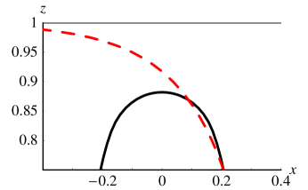
(a)  (b)

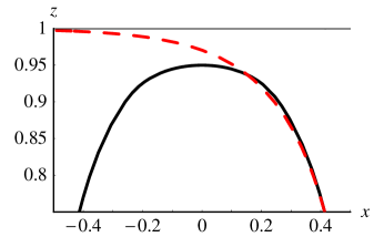
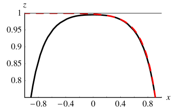
(c)  (d)

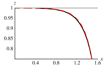
Figure 5: Cross sections of the string world sheet at times (a) $t=0.25$, (b) $t=0.5$, (c) $t=1.1$ and (d) $t=1.8$ (in units where $u_{h}=\pi T=1$), for point-like initial conditions, constant velocity boundary conditions, and a D7-brane at $z_{m}=0.75$. The velocity $v/c=0.83$ and the value of $z_{m}$ corresponds to $m/\Delta m(T)=1.28$. The red dashed line shows the constant velocity analytic single quark solution.

Through experimentation, we found that a stretching function of

$$s=\frac{1{-}z}{1-3.5\,z(1{-}z)}$$ (97)

works particularly well for this string. The $1{-}z$ factor in the numerator prevents the string worldsheet from being dragged to late times close to the horizon. The denominator ameliorates some distortion of the constant $\sigma$ and $\tau$ contours of the worldsheet for intermediate values of $z$.

4.2 Unforced motion

In this subsection we consider the motion of a quark-antiquark pair created with point-like initial conditions (94) in the absence of any external forcing. That is, we impose the usual Neumann boundary conditions along the D7-brane. A short calculation shows that the energy [given by Eq. (27)] of our point-like initial configuration is

$$E=T_{0}L^{2}\,\frac{\sqrt{1-z_{m}^{4}}}{s(z_{m})}\,\frac{A\pi}{z_{m}^{2}}\ .$$ (98)

The subsequent motion is sensitive to the value of this initial energy of the $q\bar{q}$ pair. The static potential between a heavy quark and antiquark in $\mathcal{N}\,{=}\,4$ SYM rises linearly at short distance before switching to a Coulombic form at a cross-over distance set by the inverse quark mass [40]. At non-zero temperature, the potential remains approximately Coulombic until a distance of order the inverse temperature, where (at $N_{\rm c}=\infty$) there is an abrupt transition to to a constant limiting value [which is twice the static thermal rest energy $M_{\rm rest}(T)$] [47, 48]. If the energy of the $q\bar{q}$ pair is sufficiently low, then the attractive force between the separating quarks will be strong enough to cause their trajectories to turn around, and the resulting motion will resemble an oscillator. If the energy is sufficiently high, then the quark trajectories will not have turning points and the motion will resemble a highly overdamped oscillator.

For our point-like initial conditions, the exact energy threshold for non-oscillatory motion need not equal $2M_{\rm rest}(T)$ precisely, because of the possibility of exciting internal string degrees of freedom. Numerically, however, there does indeed appear to be a divergence in the period at $E\gtrsim 2M_{\rm rest}(T)$ for these point-like initial conditions.

 

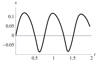
Figure 6: String endpoint as a function of time for an oscillatory solution with $z_{m}=0.50$, $E/M_{\rm rest}=1.2$, and pointlike initial conditions. To observe many oscillations, this integration tolerated a larger numerical error ($10^{-3}$ instead of $10^{-4}$ typical of the other plots in this section). The time dependent damping is comparable to the numerical error.

Numerically we do find oscillating solutions similar to the flat space expanding and contracting semi-circle (93) when $E$ is well below $2M_{\rm rest}(T)$. An example is illustrated in Figure 6. As $E$ approaches $2M_{\rm rest}(T)$ from below, the period of oscillation becomes longer and longer.

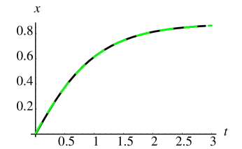
(a)  (b)

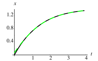
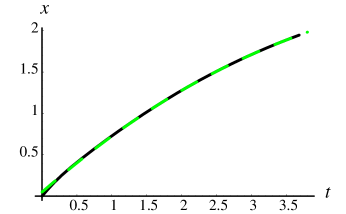
(c)  (d)

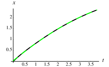
Figure 7: Plots of the position of the endpoint of the string versus time for several different D7-brane positions $z_{m}$. The string endpoint is plotted in black while the best-fit curve, as described in the text, is a green dashed line. The two curves are nearly identical. Parameters for the different solutions are: (a) $z_{m}=0.75$, $E/M_{\rm rest}=14$, (b) $z_{m}=0.50$, $E/M_{\rm rest}=6.1$, (c) $z_{m}=0.25$, $E/M_{\rm rest}=4.4$, and (d) $z_{m}=0.25$, $E/M_{\rm rest}=5.9$. Units where $u_{h}\equiv\pi T=1$ are used.

To extract information about the viscous damping of a single quark, we want to create a quark-antiquark pair with an energy greatly exceeding the binding energy,

$$E\gg 2M_{\rm rest}(T)\,,$$ (99)

so as to minimize the interaction between the quark and antiquark. Numerical solutions satisfying this large energy condition do show the expected non-oscillatory behavior. Several examples are shown in Figure 7. Solutions (a) and (b) used a stretching factor $s=(1{-}z)$, amplitude $A=0.25$, and flavor brane positions $z_{m}=0.75$ and 0.5 respectively. The masses and energies were $m/\Delta m(T)=1.28$, $M_{\rm rest}(T)/m=0.26$, and $E/M_{\rm rest}(T)=14$ for (a) and $m/\Delta m(T)=1.98$, $M_{\rm rest}(T)/m=0.51$, and $E/M_{\rm rest}(T)=6.1$ for (b). For (c), a stretching factor $s=(1{-}z)^{3/2}$, amplitude $A=0.17$, and flavor brane position $z_{m}=0.25$ were used. For this run, $m/\Delta m(T)=4.0$, $M_{\rm rest}(T)/m=0.75$, and $E/M_{\rm rest}(T)=4.4$. In the last run (d), a stretching factor of $s=(1{-}z)^{2}$, an amplitude $A=0.20$, and a flavor brane position of $z_{m}=0.25$ were used, corresponding to $E/M_{\rm rest}(T)=5.9$. Numerical error limits how far we are able to integrate in time. For initial conditions corresponding to lighter or less energetic quarks, one sees a large decrease in velocity and a clear approach to an asymptotically constant position. But for higher energies or more massive quarks (which experience less damping) numerical error prevents us from following the quark to the non-relativistic regime.

Given a quark-antiquark pair with large energy, we model each quark independently as a particle experiencing a damping force

$$\frac{dp}{dt}=-\mu\,p\,.$$ (100)

If momentum is proportional to velocity, as with non-relativistic motion, then this equation integrates to

$$v(t)=v_{0}\,e^{-\mu t}\,,\qquad x(t)=x_{\infty}-\frac{v_{0}}{\mu}\,e^{-\mu t}\,.$$ (101)

But if the relation between velocity and momentum has a relativistic form, $p\propto v/{\sqrt{1-v^{2}}}$, then equation (100) is equivalent to

$$\frac{dv}{dt}=-\mu\,v\,(1-v^{2})\,,$$ (102)

which integrates to

$$v(t) = v_{0}\bigm{/}\sqrt{v_{0}^{2}+(1-v_{0}^{2})\,e^{2\mu t}}\,,$$ (103a)

and

$$x(t) = x_{\infty}-\frac{1}{2\mu}\ln\left[\frac{1+v(t)}{1-v(t)}\right].$$ (103b)

To test the validity of this description and extract information on the damping rate $\mu$ we fit the numerical results for the position of the string endpoint to Eq. (103), treating $\mu$, $\ln(1-v_{0}^{2})$ and $x_{\infty}$ as free parameters. As shown in Figure 7, when the large energy condition (99) holds the resulting fit, using the form (103), is quite good for all $\tau$, although we do see some minor deviations at small $\tau$. In contrast, fits of these large energy solutions to the simple exponential form (101) are somewhat worse.

The fact that fits using Eq. (103) are so good supports the presumed relativistic relation between $p$ and $v$ together with a friction coefficient $\mu$ that is independent of $p$. We are following the evolution of the quark over typically a rather large momentum range as can be seen from Figure 7. The results for the extracted values of $\mu$ are nearly independent of the energy so long as $E>2M_{\rm rest}(T)$. Changing the energy by 50% or more typically only results in a few percent change in the value of $\mu$. For example, for a D7-brane at $z_{m}=0.5$, as we increase $E/M_{\rm rest}$ from 4.8 to 7.2, $\mu$ changes from 0.79 to 0.80. For the case $z_{m}=0.25$, changing $E/M_{\rm rest}$ from 4.4 to 5.9 changes $\mu$ from 0.325 to 0.326.

$\quad\mu/\pi T$ $\displaystyle\frac{m}{\Delta m(T)}$ $z_{m}$ numeric QNM 5.00 0.20 0.250 0.25 4.00 0.25 0.325 0.32 3.12 0.32 0.44 0.44 2.49 0.4 0.59 0.59 1.98 0.5 0.80 0.80 1.64 0.6 1.02 1.04 1.28 0.75 1.40 1.42

Table 2: The friction coefficient $\mu$ for various values of quark mass $m$. The quasinormal mode (QNM) results were calculated using the linear analysis of Section 3.4, while the numeric results come from the full time dependent numerics discussed in this Section.

Table 2 compares the values of $\mu$ from the quasinormal mode calculation of Section 3.4 to the best fits of our numerical integrations. The numbers are astonishingly close, giving us confidence in the linear analysis. The results begin to differ by a few percent for small mass quarks. It is not a-priori clear what causes this discrepancy. The extraction of the energy loss rate may be affected by the interaction with the other quark, but that should produce a correction of the opposite sign. There may be small thermal corrections to the relation between momentum and velocity, or residual momentum dependence in the damping rate. Conceivably, there could be nonlinear effects that are absent in the quasinormal mode analysis but which reappear in this full dynamical simulation and are relevant even at (accessibly) late times. Or this small discrepancy may reflect residual errors in our numerical integration.

5 Discussion

Let us close with a discussion of the validity of our approximations. The classical treatment of the string is justified as long as the string is much longer than a string length; quantum fluctuations will be suppressed by powers of $\ell_{s}/R$ where $R$ denotes the characteristic length of the string. All the single quark solutions we considered had strings with length of order $L$, the AdS curvature radius, or larger. As one lowers the quark mass toward the critical value $m_{\rm c}\approx 0.92\,\Delta m(T)$, the D7-brane approaches but does not quite reach the horizon. The shortest string one can get (with $m\geq m_{\rm c}$) has a length of about $0.02L$. Since $L=\lambda^{\frac{1}{4}}\,\ell_{s}$, we see that for sufficiently large $\lambda$, quantum fluctuations of the string are always suppressed. Hence, a classical treatment of the string dynamics is valid for sufficiently large $\lambda$ as long as the quark mass exceeds the critical value $m_{\rm c}$.

For applications to QCD, however, one may be interested in large but not asymptotically huge values of the ’t Hooft coupling, perhaps $\lambda\approx 20$ (corresponding to $\alpha_{\rm s}\approx 0.5$). In this regime, the condition $R\gg\ell_{s}$ can become non-trivial and for masses near the critical value $m_{\rm c}$ (which is about 2.2 $T$ for $\lambda\approx 20$) quantum fluctuations of the string will be important.

Another phenomenon that has not appeared in our discussion up to now is Brownian motion. Any dissipative thermal system must also have fluctuations, as shown by the fluctuation-dissipation theorem. In particular, a quark (of finite mass) initially at rest in the plasma should not be able to remain at rest. It will undergo Brownian motion and diffuse away from its starting point. Over a time $t$ it will travel a distance $\Delta x\sim\sqrt{Dt}$. The diffusion constant $D$ is directly related to the viscous drag,

$$D=\frac{T}{\mu M}\,.$$ (104)

This physics is missing in our classical treatment of string dynamics. A motionless string stretching from the D7-brane to the horizon is a solution to the equations of motion, and there is no obvious reason for the string endpoint to move at all. This straight motionless string clearly represents a quark at rest in the plasma.

The reason we do not see Brownian motion is due to the non-uniform nature of the large $\lambda$ and large time limits. For a quark initially moving with some $O(1)$ velocity $v$, stochastic Brownian motion will be unimportant until sufficiently late times. To see this explicitly, one can use the Langevin equation

$$\dot{\vec{p}}=-\mu\,\vec{p}+\vec{\xi}(t)$$ (105)

to model the behavior of the quark. The required assumptions underlying this description are discussed below. Here $\vec{\xi}(t)$ is stochastic white noise, with variance

$$\langle\xi_{i}(t)\xi_{j}(t^{\prime})\rangle=C\,\delta_{ij}\,\delta(t{-}t^{\prime})\,.$$ (106)

Calculating the mean square momentum at time $t$ gives

$$\langle p_{i}(t)p_{j}(t)\rangle=\langle p_{i}(t)\rangle\langle p_{j}(t)\rangle+\frac{C}{2\mu}\,\delta_{ij}\,(1-e^{-2\mu t})\,.$$ (107)

with $\langle\vec{p}(t)\rangle=\vec{p}(0)\,e^{-\mu t}$. At equilibrium, by equipartition, the kinetic energy $p^{2}/(2M_{\rm kin})$ of the quark must be ${\textstyle\frac{3}{2}}T$. (Note that the condition $m\geq m_{\rm c}$ automatically implies that $M_{\rm kin}\gg T$, so a non-relativistic form of kinetic energy is appropriate for quarks in equilibrium.) Requiring that the large $t$ limit of $\langle\vec{p}(t)^{2}\rangle$ equal $3TM_{\rm kin}$ shows that the strength of the noise is determined by the viscous drag,

$$C=2T\mu M_{\rm kin}(T)=2\pi T^{2}\Delta m(T)=\pi\sqrt{\lambda}\,T^{3}\,.$$ (108)

Integrating the Langevin equation (105) again to find the quark’s position, assuming non-relativistic motion and vanishing initial velocity, and computing the mean square displacement gives

$$\langle\Delta x_{i}(t)\,\Delta x_{j}(t)\rangle=\frac{C\,t}{(\mu M_{\rm kin})^{2}}\;\delta_{ij}\big{[}1+\mathcal{O}\big{(}1/(\mu t)\big{)}\big{]}\,.$$ (109)

This must equal the classic result $\langle\Delta x_{i}(t)\,\Delta x_{j}(t)\rangle=2D\,t\,\delta_{ij}$ for the variance of the probability distribution $P(\Delta\vec{x},t)=(4\pi Dt)^{-3/2}\,e^{-\Delta\vec{x}^{2}/(4Dt)}$ generated by a diffusion equation with diffusion constant $D$. Combining Eqs. (108) and (109) gives the stated value (104) for the diffusion constant.

For diffusive effects to be negligible, we require the second term of (107) to be small compared to the first term, giving an upper bound on the time over which a deterministic treatment of quark motion is valid,

$$t<t_{B}\equiv\frac{1}{2\mu}\ln\left(1+\frac{2K.E.}{3T}\right),$$ (110)

where $K.E.={\textstyle\frac{1}{2}}M_{\rm kin}\,v_{0}^{2}$ is the kinetic energy of the quark at time zero. At the same time, for Eq. (105) to adequately model the energy loss of the quark, quantum uncertainty in its kinetic energy must be negligible compared to the change in the kinetic energy which we wish to resolve. This imposes a lower limit on the time during which our classical description is valid, namely $1/t\ll\mu t\,(K.E.)$, or

$$t\gg t_{Q}\equiv\left[{\mu\times(K.E.)}\right]^{-1/2}\,.$$ (111)

Our analysis requires that $t_{Q}\ll t\ll t_{B}$. Using $\mu\sim\Delta m(T)T/M_{\rm kin}$, this condition may be rewritten as

$$\sqrt{\frac{\Delta m}{M_{\rm kin}}}\ll\sqrt{\frac{K.E.}{T}}\>\ln\left(1+\frac{2K.E.}{3T}\right).$$ (112)

This inequality is most stringent for the lightest (accessible) quarks with $m$ near $m_{\rm c}$ and $M_{\rm kin}\approx{\textstyle\frac{1}{2}}\Delta m(T)$. Hence the required large separation between the quantum and diffusive time scales is valid as long as the initial kinetic energy of the quark is large compared to the temperature,

$$K.E.\equiv{\textstyle\frac{1}{2}}M_{\rm kin}\,v_{0}^{2}\gg T\,.$$ (113)

For a quark mass near the critical limit $m_{\rm c}$, this is equivalent to the requirement that the initial velocity satisfy

$$v_{0}\gg\lambda^{-1/4}\,.$$ (114)

A point to be emphasized is that the classical treatment of quark dynamics underlying all results in Table 2 is valid provided $\lambda$ is sufficiently large.

The result (107) for momentum fluctuations also allows one to relate the rate of change of the mean square transverse momentum to the noise, and hence to the viscous drag,

$$\frac{d}{dt}\left\langle\vec{p}_{\perp}(t)^{2}\right\rangle\Big{|}_{t=0}=2C=4T\mu M_{\rm kin}(T)=2\pi\sqrt{\lambda}\,T^{3}\,.$$ (115)

This characterizes the diffusion in transverse momentum of a quark propagating through the plasma. However, the simple connection (115) between transverse momentum diffusion and viscous drag relies on the validity of the Langevin equation (105) with isotropic white noise (106) for modeling the stochastic force fluctuations acting on the quark. If the stochastic force fluctuations have significant momentum dependence, or non-Gaussian correlations, then this simple description will not be adequate. One can argue that the simple Langevin description is valid for non-relativistic motion, $v\ll 1$. Whether it remains valid for arbitrary momentum is not completely clear. At weak coupling, both the viscous drag and the noise variance acquire significant velocity dependence for $\mathcal{O}(1)$ values of rapidity [11]. Since we find no velocity dependence in the friction coefficient $\mu$ at strong coupling, it seems plausible that there will also be negligible velocity dependence in the variance of the force fluctuations, even for relativistic motion. However, this has not been directly verified.

Note Added:

Several related papers [53, 54, 55] have very recently appeared which overlap with portions of our analysis. The quark diffusion constant found in Ref. [54] agrees with our value (12). The result of Ref. [53] for the jet quenching parameter $\hat{q}$ does not agree with our result (13). However, these authors are addressing a different physical question involving radiative energy loss of a lightlike projectile. Interestingly, their result has the same parametric dependence as our result (115), but with a coefficient which is 15% smaller.

Appendix A Other solutions

In this appendix we briefly discuss other stationary string solutions in the $AdS_{5}$-black hole background. As we showed in Section 3.3, the ansatz $x(u,t)=x(u)+vt$ reduces the string equation of motion to the ordinary differential equation (35) with a first integral (38). The numerator in the expression (38) vanishes at $u_{c}=(1-v^{2})^{-1/d}u_{h}$, while (for $d=4$) the denominator vanishes at $u_{0}=(u_{h}^{4}+C^{2}v^{2})^{1/4}$. The previously discussed single quark solution requires $u_{c}=u_{0}$, so that $x^{\prime}$ is non-vanishing and non-singular everywhere between the horizon and the boundary. But if these two radii do not coincide, one can still find solutions with $-g$ everywhere positive on the worldsheet. If $u_{0}>u_{c}$, then the physical solution lives entirely in the $u>u_{0}$ part of space, depicted on the left in Figure 8. This configuration corresponds to an infinitely heavy external quark/antiquark pair at finite temperature, moving at a common velocity $v$. For a static quark/antiquark pair, it was found in Ref. [47, 48] that the solution only exists for a bounded range of quark/antiquark separations $l$. At zero velocity the largest separation $l_{max}$ is achieved when $u_{0}$ approaches $u_{h}$. At non-zero velocity, this solution ceases to exist beyond $u_{0}=u_{c}$.

Alternatively, if $u_{0}<u_{c}$ then the solution lives entirely in the region between $u_{0}$ and the horizon, as depicted on the right in Figure 8. One might think that this string solution could represent some coherent gluonic excitation. But since the momentum is outgoing on one end of the string, and ingoing on the other, we believe this solution is unphysical.

Figure 8: Left: Semiclassical solutions corresponding to a quark/antiquark pair with a fixed spatial separation moving through the finite temperature medium at constant speed. Right: A stationary solution in which the string moves at constant velocity outside the horizon. One end of the string satisfies physical (outgoing) boundary conditions at the horizon, but the other end does not. Hence, this solution is unphysical.

Figure 9: A straight, moving string solution corresponding to a light-heavy meson (in a multi-flavor theory) moving through the thermal medium at constant velocity.

Finally, yet another very simple solution is a straight string, $x=vt$, moving at constant velocity. We argued in Section 3 that such a string, stretching from $u_{m}$ down to the horizon and moving at any non-zero velocity, is not physical. However, if one considers a theory with two flavors of quarks with different masses, so that the gravitational description has two D7-branes at differing radial positions $u_{m_{1}}$ and $u_{m_{2}}$, then one can regard the portion of this trivial solution lying between $u_{m_{1}}$ and $u_{m_{2}}$ as describing a moving light-heavy meson. Figure 9 depicts this configuration. The solution is physical provided $u_{m_{1}}$ and $u_{m_{2}}$ are both greater than $u_{c}$. This condition shows that, for given quark masses, there is a maximum velocity with which such a color-singlet meson can move through the medium without experiencing any drag (at leading order in $1/N_{c}$ and $\lambda\to\infty$),

$$v^{2}<1-(u_{h}/u_{m_{<}})^{d}\,,$$ (116)

where $u_{m_{<}}$ is the lesser of $u_{m_{1}}$ and $u_{m_{2}}$.

Appendix B Quasinormal modes in $d=2$

In $d=2$, the metric function $h(u)=u^{2}-u_{h}^{2}$ and the resulting linear equation (54) can be solved analytically. The most general solution is

$$x(y,t)=e^{-\mu t}f(y)=e^{-\mu t}\left(c_{P}\,P_{1}^{\gamma}(y)/y+c_{Q}\,Q_{1}^{\gamma}(y)/y\right),$$ (117)

where we have introduced the dimensionless quantities $\gamma=\mu/u_{h}$ and $y=u/u_{h}$, and $P^{\gamma}_{1}$ and $Q^{\gamma}_{1}$ are associated Legendre functions. (We follow the conventions in Gradshteyn and Ryzhik [56].) The horizon is at $y=1$, and the boundary is out at $y\rightarrow\infty$. In order to study the behavior of $P^{\gamma}_{1}$ and $Q^{\gamma}_{1}$ at large $y$, and for $y$ close to 1, it is convenient to use the relation to hypergeometric functions. The associated Legendre functions $P^{\gamma}_{1}$ and $Q^{\gamma}_{1}$ are uniquely defined for $1<y<2$ and $y>1$, respectively, as

$$P^{\gamma}_{1}(y) = \frac{1}{\Gamma(1{-}\gamma)}\left(\frac{y+1}{y-1}\right)^{\gamma/2}{}_{2}F_{1}\left(-1,2,1{-}\gamma;{\textstyle\frac{1}{2}}{-}{\textstyle\frac{y}{2}}\right)\,,$$ (118)

$$Q^{\gamma}_{1}(y) = {\textstyle\frac{1}{3}}{e^{i\gamma\pi}\,\Gamma(2{+}\gamma)}\left(1-y^{-2}\right)^{\gamma/2}y^{-2}\;{}_{2}F_{1}\left({\textstyle\frac{\gamma}{2}}+{\textstyle\frac{3}{2}},{\textstyle\frac{\gamma}{2}}+1,{\textstyle\frac{5}{2}};y^{-2}\right).$$ (119)

These expressions may be used to evaluate $P^{\gamma}_{1}(y)$ for $y$ close to 1 and $Q^{\gamma}_{1}(y)$ at large $y$. To evaluate $P^{\gamma}_{1}(y)$ at large $y$ and $Q^{\gamma}_{1}(y)$ close to 1 one can use hypergeometric identities to find (see also Ref. [56]):

$$P^{\gamma}_{1}(y) = \frac{1}{3\Gamma(-1{-}\gamma)}\left(1-y^{-2}\right)^{\gamma/2}\,y^{-2}\;{}_{2}F_{1}\left({\textstyle\frac{\gamma}{2}}{+}{\textstyle\frac{3}{2}},{\textstyle\frac{\gamma}{2}}{+}{\textstyle\frac{1}{2}},{\textstyle\frac{5}{2}};y^{-2}\right)$$ (120)

$${}+\frac{1}{\Gamma(2{-}\gamma)}\left(1-y^{-2}\right)^{\gamma/2}\,y\;{}_{2}F_{1}\left({\textstyle\frac{\gamma}{2}},{\textstyle\frac{\gamma}{2}}{-}{\textstyle\frac{1}{2}},-{\textstyle\frac{1}{2}};y^{-2}\right),$$

$$Q^{\gamma}_{1}(y) = {\textstyle\frac{1}{2}}{e^{i\gamma\pi}}\biggl{[}\Gamma(\gamma)\left(\frac{y+1}{y-1}\right)^{\gamma/2}{}_{2}F_{1}\left(-1,2,1{-}\gamma;{\textstyle\frac{1}{2}}{-}{\textstyle\frac{y}{2}}\right)$$ (121)

$$\qquad{}+\frac{\Gamma(-\gamma)\Gamma(2{+}\gamma)}{\Gamma(2{-}\gamma)}\left(\frac{y-1}{y+1}\right)^{\gamma/2}{}_{2}F_{1}\left(-1,2,1{+}\gamma;{\textstyle\frac{1}{2}}{-}{\textstyle\frac{y}{2}}\right)\biggr{]}\ .$$

Close to the horizon we find that $Q^{\gamma}_{1}$ is a linear combination of a solution that goes as $(y{-}1)^{\gamma/2}$ and one that goes as $(y{-}1)^{-\gamma/2}$. According to Eq. (55), when combined with $e^{-\mu t}$ time dependence the former is in-going while the latter is outgoing. On the other hand, $P^{\gamma}_{1}$ only has a $(y{-}1)^{-\gamma/2}$ term and hence is the purely outgoing solution. So to find quasinormal modes we can focus on the $P^{\gamma}_{1}$ solution only, and set $c_{Q}=0$.

Imposing Neumann boundary conditions at a flavor brane, the quasinormal modes are given by solutions to

$$f^{\prime}(y)\big{|}_{y=y_{m}}=\partial_{y}(P_{1}^{\gamma}(y)/y)\big{|}_{y=y_{m}}=0.$$ (122)

For large $y_{m}$ we can expand the hypergeometric functions to obtain

$$f(y)=\frac{1}{\Gamma(2{-}\gamma)}\left[1-{\textstyle\frac{1}{2}}{\gamma^{2}}y^{-2}+{\cal O}\left({\gamma^{4}}y^{-4}\right)\right]+\frac{y^{-3}}{3\Gamma(-1{-}\gamma)}\left[1+{\textstyle\frac{1}{10}}(3+9\gamma+\gamma^{2})\,y^{-2}+{\cal O}\left(y^{-4}\right)\right].$$ (123)

Assuming that $\gamma\sim 1/y_{m}$, we have kept all terms up to order $y_{m}^{-7}$. This assumption will be justified presently. From this asymptotic expansion, it follows that

$$f^{\prime}(y_{m})=\frac{y_{m}^{-3}}{\Gamma(-1{-}\gamma)}\left[\frac{\gamma}{1{-}\gamma^{2}}\left(1+{\textstyle\frac{1}{2}}\,y_{m}^{-2}\right)-y_{m}^{-1}-\left({\textstyle\frac{1}{2}}{+}{\textstyle\frac{3\gamma}{2}}\right)y_{m}^{-3}+{\cal O}\left(y_{m}^{-5}\right)\right].$$ (124)

Solving $f^{\prime}(y_{m})=0$ for $y_{m}$ yields the asymptotic expression $y_{m}=\frac{1}{\gamma}-\frac{\gamma}{2}+{\cal O}(\gamma^{2})$, which justifies a posteriori our assumption about the scaling behavior of $\gamma$. Inverting this expression for $\gamma$ yields

$$\gamma=\frac{1}{y_{m}}-\frac{1}{2\,y_{m}^{3}}+{\cal O}\left(y_{m}^{-4}\right)\,.$$ (125)

The corresponding quasinormal mode wavefunction $f(y)$ is plotted in Figure 10 for $y_{m}=10$.

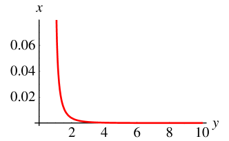
Figure 10: Quasinormal mode wavefunction $f(y)$ for a mass corresponding to $y_{m}=10$.

Appendix C Numerical error

To perform the numerical integration in Section 4, we used the NDSolve routine provided by Mathematica [52] and checked for numerical error in a variety of ways. We used the spatial error estimate provided by NDSolve, we checked the constraint equations, and we compared the numerical integration results for different grid spacings.

The routine NDSolve produces a warning if its internal spatial error estimate exceeds a threshold. None of the numerical results we present here generated such warnings. This spatial error estimate is formed by considering the final step in the numerical propagation. One additional time step is made both with the original grid and with a coarser grid with half the number of grid points. Using the Richardson extrapolation formula, Mathematica produces a warning if the difference $\frac{|y_{2}-y_{1}|}{2^{p}-1}>10$, where $y_{2}$ and $y_{1}$ are the resulting values of the function for the two different choices of grid and $p$ is the order of the discretization routine that converts derivatives into differences, the default value of which is $p=4$. The norm $|y_{2}{-}y_{1}|$ involves a scaled sum over the difference between $y_{2}$ and $y_{1}$ which the documentation of NDSolve does not describe in detail.

We made our own rough estimates of the numerical error by numerically integrating each example twice with two different grids. If the first grid was specified to have a minimum number of points $n$, the second grid would have a minimum of $2n$ points. The (absolute) difference between the two integrations was kept under about $10^{-4}$.

The constraint equations (91), if satisfied by the initial conditions, should remain satisfied at all later times. But unless special steps are taken when converting derivatives into finite differences, the differencing scheme will no longer preserve the constraint equations exactly. The extent to which the constraint equations are satisfied at later times is thus an indirect measure of the accumulated numerical error. In the numerical results presented here, we checked the constraints at a handful of points and found that they differed from zero only by about $10^{-6}$.

References

- [1] B. Svetitsky, Diffusion of charmed quark in the quark-gluon plasma, Phys. Rev. D37 (1988) 2484–2491.
- [2] E. Braaten and M. H. Thoma, Energy loss of a heavy quark in the quark-gluon plasma, Phys. Rev. D44 (1991) 2625–2630.
- [3] M. G. Mustafa, D. Pal, D. K. Srivastava, and M. Thoma, Radiative energy-loss of heavy quarks in a quark-gluon plasma, Phys. Lett. B428 (1998) 234–240, [nucl-th/9711059].
- [4] R. Baier, Y. L. Dokshitzer, A. H. Mueller, and D. Schiff, Quenching of hadron spectra in media, JHEP 09 (2001) 033, [hep-ph/0106347].
- [5] Y. L. Dokshitzer and D. E. Kharzeev, Heavy quark colorimetry of QCD matter, Phys. Lett. B519 (2001) 199–206, [hep-ph/0106202].
- [6] S. Jeon and G. D. Moore, Energy loss of leading partons in a thermal QCD medium, Phys. Rev. C71 (2005) 034901, [hep-ph/0309332].
- [7] M. G. Mustafa and M. H. Thoma, Quenching of hadron spectra due to the collisional energy loss of partons in the quark gluon plasma, Acta Phys. Hung. A22 (2005) 93–102, [hep-ph/0311168].
- [8] N. Armesto, C. A. Salgado, and U. A. Wiedemann, Medium-induced gluon radiation off massive quarks fills the dead cone, Phys. Rev. D69 (2004) 114003, [hep-ph/0312106].
- [9] M. Djordjevic and M. Gyulassy, Where is the charm quark energy loss at RHIC?, Phys. Lett. B560 (2003) 37–43, [nucl-th/0302069].
- [10] M. Djordjevic and M. Gyulassy, Heavy quark radiative energy loss in QCD matter, Nucl. Phys. A733 (2004) 265–298, [nucl-th/0310076].
- [11] G. D. Moore and D. Teaney, How much do heavy quarks thermalize in a heavy ion collision?, Phys. Rev. C71 (2005) 064904, [hep-ph/0412346].
- [12] M. G. Mustafa, Energy loss of charm quarks in the quark-gluon plasma: Collisional vs radiative, Phys. Rev. C72 (2005) 014905, [hep-ph/0412402].
- [13] H. van Hees and R. Rapp, Thermalization of heavy quarks in the quark-gluon plasma, Phys. Rev. C71 (2005) 034907, [nucl-th/0412015].
- [14] S. Wicks, W. Horowitz, M. Djordjevic, and M. Gyulassy, Heavy quark tomography of A + A including elastic and inelastic energy loss, nucl-th/0512076.
- [15] PHENIX Collaboration, S. S. Adler et. al., Nuclear modification of electron spectra and implications for heavy quark energy loss in Au + Au collisions at GeV, Phys. Rev. Lett. 96 (2006) 032301, [nucl-ex/0510047].
- [16] STAR Collaboration, M. Calderon de la Barca Sanchez et. al., Open charm production from d + Au collisions in STAR, Eur. Phys. J. C43 (2005) 187–192.
- [17] STAR Collaboration, A. A. P. Suaide et. al., Charm production in the STAR experiment at RHIC, Eur. Phys. J. C43 (2005) 193–200.
- [18] E. Shuryak, Why does the quark gluon plasma at RHIC behave as a nearly ideal fluid?, Prog. Part. Nucl. Phys. 53 (2004) 273–303, [hep-ph/0312227].
- [19] E. V. Shuryak, What RHIC experiments and theory tell us about properties of quark-gluon plasma?, Nucl. Phys. A750 (2005) 64–83, [hep-ph/0405066].
- [20] D. Molnar and M. Gyulassy, Saturation of elliptic flow at RHIC: Results from the covariant elastic parton cascade model MPC, Nucl. Phys. A697 (2002) 495–520, [nucl-th/0104073].
- [21] T. Hirano, Hydrodynamic models, J. Phys. G30 (2004) S845–S852, [nucl-th/0403042].
- [22] D. Teaney, J. Lauret, and E. V. Shuryak, A hydrodynamic description of heavy ion collisions at the SPS and RHIC, nucl-th/0110037.
- [23] D. Teaney, J. Lauret, and E. V. Shuryak, Flow at the SPS and RHIC as a quark gluon plasma signature, Phys. Rev. Lett. 86 (2001) 4783–4786, [nucl-th/0011058].
- [24] P. F. Kolb, P. Huovinen, U. W. Heinz, and H. Heiselberg, Elliptic flow at SPS and RHIC: From kinetic transport to hydrodynamics, Phys. Lett. B500 (2001) 232–240, [hep-ph/0012137].
- [25] P. Huovinen, P. F. Kolb, U. W. Heinz, P. V. Ruuskanen, and S. A. Voloshin, Radial and elliptic flow at RHIC: Further predictions, Phys. Lett. B503 (2001) 58–64, [hep-ph/0101136].
- [26] D. Molnar and P. Huovinen, Dissipation and elliptic flow at RHIC, Phys. Rev. Lett. 94 (2005) 012302, [nucl-th/0404065].
- [27] D. Teaney, Effect of shear viscosity on spectra, elliptic flow, and Hanbury Brown-Twiss radii, Phys. Rev. C68 (2003) 034913.
- [28] P. F. Kolb and U. W. Heinz, Hydrodynamic description of ultrarelativistic heavy-ion collisions, nucl-th/0305084.
- [29] P. Petreczky and D. Teaney, Heavy quark diffusion from the lattice, Phys. Rev. D73 (2006) 014508, [hep-ph/0507318].
- [30] J. M. Maldacena, The large limit of superconformal field theories and supergravity, Adv. Theor. Math. Phys. 2 (1998) 231–252, [hep-th/9711200].
- [31] E. Witten, Anti-de Sitter space and holography, Adv. Theor. Math. Phys. 2 (1998) 253–291, [hep-th/9802150].
- [32] S. S. Gubser, I. R. Klebanov, and A. M. Polyakov, Gauge theory correlators from non-critical string theory, Phys. Lett. B428 (1998) 105–114, [hep-th/9802109].
- [33] E. Witten, Anti-de Sitter space, thermal phase transition, and confinement in gauge theories, Adv. Theor. Math. Phys. 2 (1998) 505–532, [hep-th/9803131].
- [34] P. Kovtun, D. T. Son, and A. O. Starinets, Viscosity in strongly interacting quantum field theories from black hole physics, Phys. Rev. Lett. 94 (2005) 111601, [hep-th/0405231].
- [35] S. S. Gubser, I. R. Klebanov, and A. W. Peet, Entropy and temperature of black 3-branes, Phys. Rev. D54 (1996) 3915–3919, [hep-th/9602135].
- [36] P. Kovtun, D. T. Son, and A. O. Starinets, Holography and hydrodynamics: Diffusion on stretched horizons, JHEP 10 (2003) 064, [hep-th/0309213].
- [37] A. Buchel, On universality of stress-energy tensor correlation functions in supergravity, Phys. Lett. B609 (2005) 392–401, [hep-th/0408095].
- [38] A. Karch and E. Katz, Adding flavor to AdS/CFT, JHEP 06 (2002) 043, [hep-th/0205236].
- [39] S.-J. Sin and I. Zahed, Holography of radiation and jet quenching, Phys. Lett. B608 (2005) 265–273, [hep-th/0407215].
- [40] M. Kruczenski, D. Mateos, R. C. Myers, and D. J. Winters, Meson spectroscopy in AdS/CFT with flavour, JHEP 07 (2003) 049, [hep-th/0304032].
- [41] J. Babington, J. Erdmenger, N. J. Evans, Z. Guralnik, and I. Kirsch, Chiral symmetry breaking and pions in non-supersymmetric gauge/gravity duals, Phys. Rev. D69 (2004) 066007, [hep-th/0306018].
- [42] A. O’Bannon and A. Karch, Chiral transition of N=4 super Yang-Mills with flavor on a 3-sphere, hep-th/0605120.
- [43] D. Mateos, R. C. Myers, and R. M. Thomson, Holographic phase transitions with fundamental matter, hep-th/0605046.
- [44] T. Albash, V. Filev, C. V. Johnson, and A. Kundu, A topology-changing phase transition and the dynamics of flavour, hep-th/0605088.
- [45] R. Baier, Y. L. Dokshitzer, A. H. Mueller, S. Peigne, and D. Schiff, Radiative energy loss and -broadening of high energy partons in nuclei, Nucl. Phys. B484 (1997) 265–282, [hep-ph/9608322].
- [46] O. Aharony, S. S. Gubser, J. M. Maldacena, H. Ooguri, and Y. Oz, Large field theories, string theory and gravity, Phys. Rept. 323 (2000) 183–386, [hep-th/9905111].
- [47] A. Brandhuber, N. Itzhaki, J. Sonnenschein, and S. Yankielowicz, Wilson loops in the large limit at finite temperature, Phys. Lett. B434 (1998) 36–40, [hep-th/9803137].
- [48] S.-J. Rey, S. Theisen, and J.-T. Yee, Wilson-Polyakov loop at finite temperature in large gauge theory and anti-de Sitter supergravity, Nucl. Phys. B527 (1998) 171–186, [hep-th/9803135].
- [49] J. M. Maldacena, Wilson loops in large field theories, Phys. Rev. Lett. 80 (1998) 4859–4862, [hep-th/9803002].
- [50] S.-J. Rey and J.-T. Yee, Macroscopic strings as heavy quarks in large gauge theory and anti-de Sitter supergravity, Eur. Phys. J. C22 (2001) 379–394, [hep-th/9803001].
- [51] D. T. Son and A. O. Starinets, Minkowski-space correlators in AdS/CFT correspondence: Recipe and applications, JHEP 09 (2002) 042, [hep-th/0205051].
- [52] S. Wolfram, Mathematica Version 5.2. Wolfram Research, 2005.
- [53] H. Liu, K. Rajagopal, and U. A. Wiedemann, Calculating the jet quenching parameter from AdS/CFT, hep-ph/0605178.
- [54] J. Casalderrey-Solana and D. Teaney, Heavy quark diffusion in strongly coupled N=4 Yang Mills, hep-ph/0605199.
- [55] S. S. Gubser, Drag force in AdS/CFT, hep-th/0605182.
- [56] I. Gradshteyn and I. Ryzhik, Table of Integrals, Series and Products. Academic Press, 1994.